1. Art and Diseño

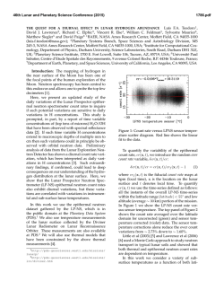
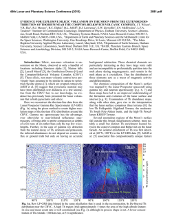
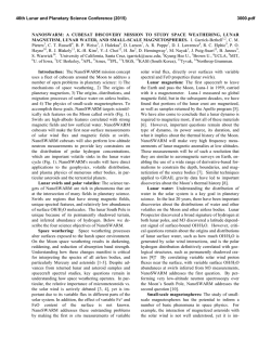
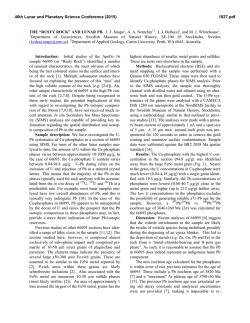
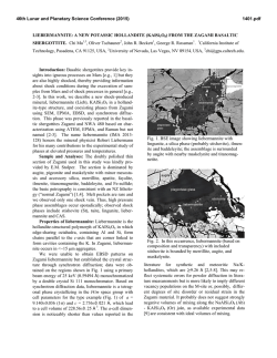
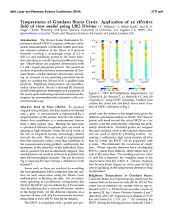
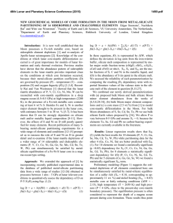
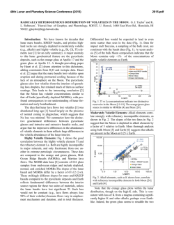
Research on Impact P rocess of Lander Footpad against Simulant Lunar
Soils
Bo HUANG, Zhujin JIANG, Peng LIN, Daosheng LING
Bo HUANG
MOE Key Laboratory of Soft Soils and Geoenvironmental Engineering, Department of Civil Engineering,
Zhejiang University, Hangzhou, 310058, China
Email: [email protected]
Zhujin JIANG
MOE Key Laboratory of Soft Soils and Geoenvironmental Engineering, Department of Civil Engineering,
Zhejiang University, Hangzhou, 310058, China
Email: [email protected]
Peng LIN
State Key Laboratory of Hydroscience and Engineering, Tsinghua University, Beijing 100084, China
Email: [email protected]
Daosheng LING (Corresponding author)
MOE Key Laboratory of Soft Soils and Geoenvironmental Engineering, Department of Civil Engineering,
Zhejiang University, Hangzhou, 310058, China
Email: [email protected]
Tel:86-571-88208756
Fax:86-571-88208793
Abstract：
The safe landing of a moon lander and the performance of the precise instruments it carries may be
affected by too heavy an impact on touchdown. Accordingly, landing characteristics have become an
important research focus. Described in this paper are model tests carried out using simulated lunar soils
of different relative densities ( called „simulant‟ lunar soils below), with a scale reduction factor of 1/6 to
consider the relative gravities of the Earth and Moon. In the model tests, the lander was simplified as an
impact column with a saucer-shaped footpad with various impact landing masses and velocities. Based on
the test results, the relationships between the footpad peak feature responses and impact kinetic energy
have been analyzed. Numerical simulation analyses were also conducted to simulate the vertical impact
process. A 3D dynamic finite element model was built for which the material parameters were obtained
from laboratory test data. When compared with the model tests, the numerical model proved able to
effectively simulate the dynamic characteristics of the axial forces, accelerations and penetration depths
of the impact column during landing. This numerical model can be further used as required for simulating
oblique landing impacts.
Keywords: lunar lander; footpad; vertical impact; simulant lunar soil; model test; numerical simulation.
1
Introduction
Landing on the Moon has long been a dream of mankind. In the 1960s, dozens of lunar exploration
activities were carried out by the USA and the Soviet Union, which opened a new era of human
exploration of the moon. Moon landings have led to many lunar surface activities, such as lunar surface
travelling, drilling, excavating, establishing shallow foundations and the extraction of resources.
During the landing process, the response to impact of the footpad is very important. The footpad is
the part of the lunar- lander directly touching and impacting the lunar soil. Ever since the 1970s, scientists,
mainly in the USA, have carried out much research on the impact process during landing [1~2], in order to
verify the stability and reliability of the lander, as it actually lands. These studies have investigated the
influence of such as types of simulant lunar soils, impact velocities, model scales, on impact response.
Since it is hard to measure the real impact procedure of moon lander, just as Stiros and Psimoulis
[3]
did
on the moving train during its passage over a railway bridge, the landing- impact model tests and
numerical simulation [4~7] have the same importance. In China, since completion of the first stage of the
lunar exploration mission, moon landing preparation work has been an ongoing task. A major task in the
design and optimization of the lunar lander is to determine the loads, the footpad bears, and the landing
penetration depth [8].
In this paper, studies of the interaction between the footpad and simulant lunar soils are described in
detail. The studies combined model tests and numerical simulation analyses similar to other experimental
and numerical studies in civil structural engineering
[9~11]
. Based on a prototype vertical impact model
test apparatus, 1/6 subscale model experiments were carried out, focusing on vertical impact landing.
The time- history characteristics and peak characteristics of the footpad during impact were studied as
well as the variations in axial forces and footpath penetration depths for different relative densities of
simulant lunar soil, different impact masses and impact velocities. Described in this paper is also a
dynamic simulation approach for analyzing the footpad impact process using a 3D dynamic finite
element method. The commercial software Abaqus
[12]
was selected for the study for its friendly
application development environment and powerful dynamics analysis capabilities. The footpad is
modeled as a rigid block with specified mass and velocity, while the lunar soil is represented by the
Mohr-Coulomb model which conforms to the non-associative flow rule and can take into account strain
softening properties. The soil- footpad interaction is assumed to conform to the ideal Elasto-Plastic
relationship. The material parameters used in the numerical model were obtained from the monotonic
and cyclic tests on a simulant lunar soil named TJ-1. A comparison with model test results, proved the
numerical model to be valid.
2
Vertical impact model test
2.1 Properties of simulant lunar soil ( named TJ-1) used in the model test
Tens of individual lunar explorations have brought back a total mass of about 382.0 kg of lunar
regolith[13], and following testing of these lunar soils, Vinogradov et al.[14], Costes et al.[15], Mitchell et
al.[16], Carrier et al.[17~18], McKay et al.[4] have reported the properties of lunar soil in detail. Several lunar
soil simulants have since been developed and used widely in experiments, including MLS-1, ALS, JSC-1,
FJS-1, MKS-1, LSS, GRC-1, etc.[19~25] Chinese scientists have also developed several lunar soil
simulants, including NAO-1[26], CAS-1[27] and TJ-1[28]. TJ-1, developed from volcanic ash, has a low
production cost and possesses good similarity to lunar soil. Thus, TJ-1 was adopted for this study.
Fig.1 S EM image of TJ-1 particles
As shown in Fig. 1, the particles of TJ-1 are multi-angular, with holes existing in large particles.
The physical and mechanical properties of TJ-1 are given in Table 1, where the property parameters of
real lunar soil are also given for comparison. The internal friction angle of lunar soil = 25~50, the
cohesion = 0.1~15kPa, and the compression index at medium compactness = 0.1~0.11 corresponding to
a normal pressure range of 12.5~100kPa. Bulk density is 1.30~2.29 g/cm3 , and the void ratio is=
0.67~2.37. Relevant values for TJ-1 are all within those ranges.
Tab.1 Comparison of properties between lunar soil and TJ-1
Soil type
Lunar soil
TJ-1
2.9~3.5(McKay, et al. [4])
2.72(Jiang[28])
3.1(Willman, et al. [29])
2.7(tested by ourselves)
Speci fic gravity
3.1(Kanamori, et al. [21])
1.35~2.15(Mitchell, et al. [16])
1.36(Jiang[28])
Bulk density
1.45~1.9(Carrier, et al.
[17-18]
)
(g/cm3 )
1.02~1.639(tested by ourselves)
1.53~1.63(Kanamori, et al. [21])
47.6°(Jiang
37°~47°(Mitchell, et al.
[28]
)
[16]
)
Friction angle(deg)
Max. :40.0°~50.9°(tested by ourselves)
25°~50°(Carrier, et al.
[30]
)
Res. :38.5°~43.6°(tested by ourselves)
0.15~15(Jaffe et al.
[31]
)
0.86(Jiang
[28]
)
Apparent Cohesion
[4]
1.0(McKay, et al. )
Max. :0~38.7(tested by ourselves)
0.1~1(Kanamori, et al. [21])
Res. :0~9.3(tested by ourselves)
(kPa)
0.086(Jiang[28])
Compression index
0.01~0.11(Gromov
[32]
)
(MPa-1 )
0.025~0.1(tested by ourselves)
Fig. 2 shows the stress-strain curves for TJ-1 obtained from triaxial tests under confining pressures
below 60kPa. As gravity on the Moon is only 1/6 of that on the earth, the overburden stresses in soil
layers lying within the impact influence range are not large. The relative densities of TJ-1 samples are
40%, 60%, 80%, representing medium, dense, very dense states respectively. Within the tested stress
range, TJ-1 soil samples exhibited strong strain-softening behaviour with increase of confining pressure
and relative density. The residual strengths were almost 60%~90% of peak strengths. Furthermore,
influenced by the engagement of soil particles that are subangular to angular in shape, the lunar soil
simulant shows large apparent cohesion properties and internal friction angle.
5
30kPa, v=0.1%
30kPa, v=1%
6
60kPa, v=1%
1-3/100kPa
60kPa, v=0.1%
Dr=80%
7
4
1-3/100kPa
2
60kPa, v=0.1%
Dr=60%
60kPa, v=1%
1-3/100kPa
8
Dr=40%
3
3
30kPa, v=0.1%
2
30kPa, v=1%
60kPa, v=0.1%
5
4
30kPa, v=0.1%
3
15kPa, v=0.1%
15kPa, v=1%
0
0
4
2
15kPa, v=0.1%
1
15kPa, v=1%
15kPa, v=1%

8
12
(a) M edium
0
0
4
1

8
12
(b) Dense
Fig. 2 Stress-strain curves of TJ-1
2.2 Test model and device
60kPa, v=1%
30kPa, v=1%
1
0
15kPa, v=0.1%
0
4

8
(c) Very Dense
12
When the footpad touches the lunar soil, the lander has to withstand a huge impact. The entire
interaction process can be divided into the 3 stages shown in Fig. 3: impacting vertically, sliding
horizontally and achieving hydrostatic equilibrium. The first two stages happen almost simultaneously.
The impacting process is the most dangerous stage, and this aspect is the focus of this paper.
Fig.3 Landing process of footpad
Fig. 4(a) shows a schematic diagram of the vertical impact test. The shock tube with a mass m,
consisting of footpad and counterweights, impacts against TJ-1 soil site at a velocity v, forming a crater
of a certain depth on the site surface. Despite the differences between the simplified model and real
landing conditions, characteristics of the dynamic interaction between the footpad and simulant lunar soil
can be obtained. Such characteristics are suitable for use in the design of the lander.
Since it is difficult to simulate the full lunar surface environment which no doubt affected the
landing interactions, the key factors which influence impact responses should be considered. The lunar
gravity is quite different from that of the Earth, by about one sixth, so a scale factor of 6 was selected for
the model tests. Scales of other regular physical quantities are given in Table 2. Zhang Ze-mei, et al.
[33]
compared the results of 1/6 scale tests when under an Earth gravity field and the full-scale tests under a
simulated lunar gravity field, showed a remarkable degree of similarity. Other scholars also have done
researches in this area [34-36]. Because of space restrictions, this paper does not detail the feasibility of the
scale selected.
Tab. 2 S imilar S cale between earth and moon
Quantities
Acceleration
Length
Velocity
Force
Stress
Mass
Scale factor
n
1/n
1
1/n2
1
1/n3
Test scale
6
1/6
1
1/36
1
1/216
A prototype landing test device, which is used to research response law of footpad in various
masses and velocities, includes impact, control and acquisition systems, and a model box, as shown in
Figs. 4 (b) and (c). The impact system consists of an overall frame, vertical slide rail and shock tube. The
shock tube has a certain mass and can fall freely along the vertical slide rail at a certain velocity to
impact the soil site in the model box, as shown in Fig. 5(a). The specified impact velocity is obtained by
adjusting the drop height.
Cylinder
Shock
tube
Footpad
dmax
v
z
TJ-1
soil site
(a) Model sketh of footpad impact vertically
Impact
system
(b) Configuration of the device
Displacemeter
Control &
acquisition
system
Shock tube
Model box
(c) Photo of the self-made apparatus
Fig. 4 Impact model and test apparatus
Fixed
lever
Shock
tube
Weights
Guide for downslide
Cylinder
Footpad
(a) Vertical slide rail
(b) Impact cylinder
Dynamometer
Equidistant
scratch lines
Accelerometer
(c)Footpad and the arrangement of test sensors on it
(d) Model box and the simulant lunar soil site
Fig.5 Detail of the apparatus component
The shock tube is composed of a cylinder, fixed lever, weights and footpad, as shown in Fig. 5(b).
The footpad, made of hard aluminum, is fixed on a fixed lever and the weights are fastened by the fixed
lever and bolts in the cylinder to avoid collision, one with the other. The impact mass is controlled by
changing the numbers of weights.
(a) Magnetostrictive displacement/speed sensor
(b) Piezoelectric dynamometer (c) Piezoelectric accelerometer
Fig.6 Transducers used in the impact test
As shown in Fig.6, there involve three kinds of high precision transducers in the impact test. Fig.6
(a) shows the magnetostrictive displacement/speed sensor produced by the MTS Systems Corporation,
type RHM1200MR021V0. It can be used to measures the changes of velocity and displacement of the
footpad simultaneously. Its displacement measurement range is 0~5000mm, with a precision of 0.001%
FSO (i.e., ±5μm). The velocity measurement range is 0~10m/s, with a precision of 0.5% FSO; its
resolution is ±0.1mm/s, and frequency response time is up to 0.2ms. Fig.6 (b) shows the piezoelectric
dynamometer produced by Jiangsu Lianneng Electronic Technology Co., Ltd. in China, type
CL-YD-320, with a measurement range of 0~5kN and an error range of ±1% FSO. Fig.6(c) shows the
uni-axial piezoelectric accelerometer produced by Kistler Group in Switzerland, type 8776A50. Its range
is 0~50g, frequency range 0.5~10000Hz, and amplitude non- linearity ±1%FSO. The accelerometer and
dynamometer are arranged, as in Fig.5(c), to measure acceleration and impact force. Two accelerometers
are set along the radial direction for mutual checking.
In the mixed-measurement system, studies have shown that there is a phase delay between the
records of different sensors
[37]
. The sensors‟ synchronization is important especially when the impact of
the landing lasts only a few milliseconds. The Compact DAQ-based data acquisition system produced by
National Instruments is used in the experiment. The system controls the state of motion and collects the
real-time dynamic response data relating to the footpad. The hardware containing a four-slot chassis
cDAQ-9174 and 32-channel acquisition module NI-9205, as shown in Fig. 7. This system features 16-bit
resolution, and a maximum sample rate of 250 kS/s. It has four 32-bit timers built in to share clocks for
the mixed-measurement systems. In the experiment, digital analog converter will record the sampling
time, up to 0.1ms. Settling time for multichannel measurements is ±120 ppm of full-scale step (±8 LSB)
with 4 μs convert interval.
Fig.7 Data acquisition system of NI
The footpad used in the experiment is modeled after some simplification on the NASA footpad
mentioned by S. Bend [2] , as shown in Fig.8.
In cm
cm
a）NAS A footpad (from S . Bend)
b）Dimensions of footpad in this test
c）Factual picture of the footpad
Fig.8 Experimental footpad
The model box, of size 399cm×49cm×50cm, consists of steel frames and plexiglass installed as side
walls to ensure overall stiffness and visibility. Equidistant scratch lines, every 5 cm, are scribed into the
surface of the plexiglass as shown in Fig. 5(d).
2.3 Experimental procedures
2.3.1 Calibration
Before the experiment, each sensor was calibrated and showed good linearity. Because of space
limitations the relevant curves are not given in this paper.
The relationship between the drop height and impact velocity was also confirmed by carrying out
drop tests. The results are shown in Fig. 9 and illustrate good repeatability. The drop height and impact
velocity relationship fits a quadratic relationship.
4
Impact velocity/m.s
-1
v=( 17.1h)
0.5
3
2
1
0
0.0
0.2
0.4
0.6
0.8
1.0
Drop height/m
Fig.9 Relation between drop height and impact velocity
2.3.2 Site preparation
Owing to the uneven distribution of lunar soil simulant particle sizes, the dry pluviation sample
preparation method causes coarse and fine particles to segregate, leading to various and undesirable
relative densities[38]. To ensure overall uniformity, the tamping method (layering, filling, compaction, and
leveling) was used to prepare soil sites with 6 layers in total, 5 cm per layer. For each relative density,
soil with a specified mass was uniformly placed into each layer and aligned with the scratch lines as
shown in Fig. 5(d). The relative densities selected in the model tests were 40%, 60% and 80%
respectively, corresponding to the density of the simulant lunar soil samples in triaxial tests.
2.3.3 Test scheme and procedures
According to the mass of the lunar lander being simulated, the shock tube mass was variously set at
1.5kg, 3.0kg and 6.0kg. Table 3 presents the impact velocities in the impact model tests, values that can
be reached in the real landing process.
Tab.3 Comparison of impact velocity
Cases
NASA test [2]
Apollo [39]
Luna 16[40]
velocity/ m·s-1
0.3~4.57
0.3~0.9
<2.4
The scheme of the impact model tests is detailed in Table 4, which mainly includes the influencing
factors of relative density, impact velocity and impact mass.
Tab.4 S cheme of the model tests
-1
Variables
Dr/%
v/m·s
value
40, 60, 80
1.0, 2.0, 4.0
m/kg
Test number
1.5, 3.0, 6.0
27
The steps taken in each test are as follows:
(1) Prepare the soil sites with a specific relative density;
(2) Lift the shock tube with a particular mass, and fasten it at the height calibrated by the
displacement meter;
(3) Turn on the acquisition system;
(4) Release the shock tube to impact soil site, and monitor and save the test data.
3 Results of the vertical impact tests
Repeated tests were conducted under the same conditions to verify the reliability of the test results.
Fig. 10 shows the time-history curves of axial force and penetration displacement, which show good
repeatability, proving that the test results are reliable.
2.5
60
2.0
50
Axial force/kN
1.5
Displacement/mm
Dr=60%
m=6.0kg
v=4m/s
40
1.0
0.5
20
0.0
-0.5
Dr=60%
m=6.0kg
v=4m/s
30
10
0
20
40
60
80
100
120
140
160
0
0
20
40
Time/ms
（a）Axial force
60
80
100
120
140
160
Time/ms
（b）Displacement
Fig.10 Time-history curves of of impact response
3.1 Site deformation
The results of 27 groups of tests indicate that the shapes of impact craters are similar and resemble a
basin. The sizes and depths of the craters, however, are different due to changes in test conditions. Larger
impact velocities generate dramatically larger and deeper craters. Fig. 11 shows the craters formed by the
shock tube impacting with different velocities on the TJ-1 simulant soil site when Dr=60%.
Fig.11 Impact craters on TJ-1 soil site (Dr=60%)
3.2 Time-related characteristics of response
The shapes of the dynamic response curves are similar even for different testing conditions. Fig. 12
gives the typical time- history dynamic response curves for the footpad, including displacement, velocity,
axial force and acceleration curves at the instant of contact, when Dr=60%, v=2 m/s and m=6 kg. It can
be seen in Fig. 12(a), that the footpad reaches the maximum penetration depth at 25 millisecond. With
the time increasing, the penetration depth initially decreases, increases later and eventually reaches
stability. This indicates that the footpad rebounds after it reaches the maximum depth, then again impacts
the simulant lunar soil site, and after further small vibrations, tends to finally become stable
The velocity time- history curve shown in Fig.12 (b) indicates that the initial high velocity is at
1ms~3ms, since at that stage gravity far overcomes the resistance of the lunar soil stimulant, before
decreasing rapidly. It then fluctuates weakly on the horizontal axis and trends to zero.
Fig.12 (c) indicates that the axial force in the footpad reaches its maximum value in the initial 5
milliseconds before reducing and creating a second peak. The resultant impulse is found to be 13.02N·s,
the integral given by the area enclosed by curve ab in Fig. 12(c), which approximately equals the change
in momentum, of 13.09 kg·m/s (based on the reduction in initial velocity 2 m/s downwards to the
velocity 0.182 m/s upwards). A comparison of Figs. 12 (c) and (a), indicates that the displacement
response lags behind that of the axial force.
As shown in Fig. 12(d), the two acceleration time-history curves recorded by the two accelerometers
set on the footpad as shown in Fig. 5(c) are in good agreement. A comparison of Figs. 12 (d) and (c),
shows that acceleration and axial force responses are in phase.
2.0
20
15
1.5
Axial Force/kN
-1
25
1.0
0.5
10
5
0
0
20
40
Time/ms
60
80
(a) Curves of displacement
100
1.5
25
1.2
20
0.9
15
0.3
0.0
0.0
-0.3
20
40
60
Time/ms
(b) Curves of velocity
80
100
Accelerometer 1
Accelerometer 2
10
0.6
-0.5
0
Acceleration/g
2.5
30
Velocity/m.s
Penetration displacement/mm
35
a
b
c
5
0
-5
0
20
40
Time/ms
60
(c) Curves of axial force
80
100
0
20
40
60
Time/ms
80
100
(d) Curves of acceleration
Fig.12 Time-history curves of contact-dynamic characteristics with Dr =60%, v=2m/s, m=6kg
The force the footpad bears during the impact process is critical for a safe landing. Fig. 13 shows the
time- history curves of axial force for various relative densities, impact velocities and impact masses.
These curves indicate that the various modes of axial force are similar, in the initial instant contact force
grows quickly to its peak value in only a few milliseconds. It then declines to a lower level and tends to
be finally equal to the weight of the shock tube.
2.8
2.8
2.4
m=3kg
v=2m/s
Axial force/kN
Axial force/kN
2.0
Dr=80%
1.6
Dr=60%
1.2
Dr=40%
0.8
2.4
2.0
v=4.0m/s
Dr=60%
m=3.0kg
1.6
1.2
Dr=60%
v=2m/s
2.0
Axial force/kN
2.4
2.8
v=2.0m/s
0.8
m=6.0kg
1.6
m=3.0kg
1.2
Second peak
0.8
Second peak
0.4
0.4
0.4
0.0
10
20
Time/ms
(a) Curves influenced by Dr
30
40
0.0
v=1.0m/s
0.0
0
0
10
20
Time/ms
30
(b) Curves influenced by velocity
40
m=1.5kg
0
10
20
Time/ms
30
40
(c) Curves influenced by impact mass
Fig.13 Time-history curves of axial force under different testing condition
Fig. 13(a) shows the axial force response to the impact for soils of 3 different densities, which
indicate that the denser the site, the larger the peak axial force and the shorter the impact duration time.
Fig. 13(b) illustrates that the axial force increases approximately linearly with increasing impact velocity
but the impact duration time increases little. Fig. 13(c) demonstrates that the bigger the impact mass, the
larger the peak axial force and the longer the impact duration time.
It is noteworthy that the axial forces remain almost unchanged in some cases in Fig. 13 between the
the two peaks over quite long periods with respect to the whole process. A similar phenomenon was
found in the foodpad impact study made by NASA [2]. This phenomenon gives proof that the simulant
lunar soil site reached a state of 'flow failure' under impact. As in soil mechanics, “flow failures are
characterized by a sudden loss of strength followed by a rapid development of large deformations [41]”.
The term 'flow failure' is adopted here to describe the phenomenon that the deformation increases
sharply when the axial force has a sharp decrease. From the present experiment, the occurrence of this
phenomenon is conditioned. When the relative density of the simulant lunar soil site is low, the flow
failure is more pronounced. For a specified relative density, the larger the impact velocity and the impact
mass, the easier it is for flow failure to occur. It can be deduced that there exists a critical impact
momentum or kinetic energy value for a simulant lunar soil site of a specified density. When less than
that critical value, the impact will not cause flow failure of the simulant lunar soil site. The explanation is
that with the footpad penetration depth increasing, if the underlying soil of the ground is not able to bear
the impact, the soil will exhibit plastic flow failure; otherwise, if the underlying soil has a relatively great
strength which is enough to carry the impact force, flow failure will not occur.
Penetration displacement is another major factor affecting landing safety. Fig. 14 shows the time
history curves of penetration displacement for Dr=60% and v=2m/s, and different impact masses. The
time of the first impact all begins from the 0 point. The variations in penetration displacement patterns
are similar, i.e., a quick increase once the lander touches the site, a rebound after reaching the peak value,
followed by a slight further impact before reaching an ultimate stability. The larger the impact mass, the
larger the peak value and ultimate stable penetration depth, and the longer the rebound duration time.
Penetration displacement/mm
35
m=6.0kg
30
25
m=3.0kg
20
m=1.5kg
15
10
Dr=60%
v=2m/s
5
0
0
20
40
Time/ms
60
80
100
Fig.14 Time-history curves of penetration displacement with Dr =60%, v=2m/s
3.3 Correlation of axial force and penetration displacement
Fig. 15(a) shows the relationship between penetration displacement and axial force for Dr=60%,
m=6 kg and different impact velocities. The curves shapes are similar. The whole curve can be divided
into 4 stages, denoted by the characters A, B, C, D, E as shown in Fig. 15(a).
The curve in stage AB is approximately linear. The axial force on the footpad is generated by the
dynamic interaction between shock tube and the compressed soil. The penetration displacement mainly
is one of elastic compression deformation of the soil during this stage. In the shearing stage BC, part of
the soil element under the footpad reaches failure, and the soil resistance decreases allowing shear
deformation to occur. That is why the slope of the curve becomes negative. In the flow failure stage CD,
due to the expansion of the affect zone surrounding the footpad, the resistance of the soil remains stable
or increases a little, but large vertical deformation occurs and the footpad is deeply pierced. Note that,
when the impact momentum or energy is smaller, there is no flow failure stage CD, as in the case of
v=1.0m/s, as shown in Fig. 15(a). In stage DE, because of the weak elastic properties of the lunar soil
simulant, the footpad rebounds even off the surface, and the axial force decreases sharply even turns
negative. After fluctuating weakly, the displacement of the footpad tends to reach the ultimate point E
and the axial force tends to equal the shock tube‟s gravity induced weight.
-1
Velocity/m.s
Axial force/kN
0.0
A
0
0.5
1.0
1.5
2.0
-0.5
0
2.5
0.0
0.5
1.0
1.5
2.0
5
5
10
B
Displacement/mm
Displacement/mm
2.5
K
v=1.0m/s
15
20
E
25
C
v=4.0m/s
D
30
35
v=2.0m/s
40
m=6.0kg,Dr=60%
m=6.0kg,Dr=60%,v=2m/s
10
15
20
N
25
45
50
M
30
55
（b）Relationship of displacement versus velocity
(a) Relationship of displacement versus axial force
Fig.15 Test result of Dr =60%, m=6kg
The velocity variation of the footpad on the vertical motion track is shown in Fig. 15(b). In the
instant of contact, the velocity increases to peak point K within a 2~3mm penetration displacement due
to the shock tube inertia. The velocity then decreases gradually until reaching the maximum penetration
displacement point M when the velocity equals zero. After fluctuating several times, it finally reaches the
ultimate penetration point N.
3.4 Peak feature of dynamic response
Other than the time-history characteristics of the footpad dynamic response in the instant of contact,
the peak values themselves are essential for the design of the lander buffering system, especially the
extent of penetration which is the stable penetration displacement. Peak values of axial force and
acceleration are also essential.
Fig. 16 and Fig. 17 show the effect of relative density on peak axial force and penetration depth,
which indicates that peak axial force increases significantly as relative density increases in all test
conditions, while penetration depth is reduced.
Axial force peak/kN
2.5
Axial force peak/kN
v=1.0m/s
v=2.0m/s
v=4.0m/s
2.0
1.5
1.0
0.5
3.0
2.5
2.0
1.5
40
50
60
70
Relative density/%
(a) In case of m=1.5kg
80
4.0
3.5
3.0
2.5
2.0
1.5
1.0
1.0
0.5
0.5
0.0
0.0
40
50
v=1.0m/s
v=2.0m/s
v=4.0m/s
4.5
v=1.0m/s
v=2.0m/s
v=4.0m/s
3.5
m=6.0kg
5.0
m=3.0kg
4.0
Axial force peak/kN
m=1.5kg
3.0
0.0
5.5
4.5
3.5
60
Relative density/%
(b) In case of m=3.0kg
70
80
40
50
60
Relative density/%
(c) In case of m=6.0kg
70
80
Fig.16 Effect of relative density on peak axial force
35
50
40
m=1.5kg
20
15
10
5
30
40
50
60
70
80
25
20
15
10
0
Relative density/%
v=1.0m/s
v=2.0m/s
v=4.0m/s
40
35
30
25
20
15
10
5
0
m=6.0kg
45
v=1.0m/s
v=2.0m/s
v=4.0m/s
Penetration depth/mm
25
m=3.0kg
35
v=1.0m/s
v=2.0m/s
v=4.0m/s
Penetration depth/mm
Penetration depth/mm
30
5
40
50
60
70
0
80
40
50
(a) In case of m=1.5kg
60
70
80
Relative density/%
Relative density/%
(b) In case of m=3.0kg
(c) In case of m=6.0kg
Fig.17 Effect of relative density on penetration depth
Fig. 18 demonstrates that peak axial force is little affected by impact mass. When the impact mass is
four times greater, peak axial force is only increased by 13%. In contrast to the influence of relative
density, penetration depth increases almost linearly as impact mass increases, as shown in Fig. 19, with
an increase to 215% of the initial lowest impact mass.
1.8
Dr=40%
1.2
v=1.0m/s
v=2.0m/s
v=4.0m/s
0.9
0.6
0.3
4
2.5
Dr=60%
2.0
Axial force peak/kN
Axial force peak/kN
Axial force peak/kN
1.5
0.0
5
3.0
v=1.0m/s
v=2.0m/s
v=4.0m/s
1.5
1.0
Dr=80%
v=1.0m/s
v=2.0m/s
v=4.0m/s
3
2
1
0.5
1
2
3
4
Impact mass/kg
5
0.0
6
0
1
(a) In case of Dr=40%
2
3
4
Impact mass/kg
5
6
(b) In case of Dr=60%
1
2
3
4
5
6
5
6
Impact mass/kg
(c) In case of Dr=80%
Fig.18 Effect of impact mass on peak axial force
v=1.0m/s
v=2.0m/s
v=4.0m/s
35
40
30
20
30
15
Dr=60%
v=1.0m/s
v=2.0m/s
v=4.0m/s
Penetration depth/mm
50
40
Dr=40%
Penetration depth/mm
Penetration depth/mm
60
25
20
15
2
3
4
5
6
Impact mass/kg
(a) In case of Dr=40%
5
1
v=1.0m/s
v=2.0m/s
v=4.0m/s
9
6
3
10
10
1
12
Dr=80%
2
3
4
Impact mass/kg
(b) In case of Dr=60%
5
6
1
2
3
4
Impact mass/kg
(c) In case of Dr=80%
Fig.19 Effect of impact mass on penetration depth
Fig. 20 shows the peak axial force is evidently affected by impact velocity; the increase ranges
around 318%~693% as impact velocity increases four times. Fig. 21 shows that the penetration depth
also increases significantly as impact velocity increases in all test conditions.
5.0
2.7
Dr=60%
Dr=40%
1.2
Axial force peak/kN
Axial force peak/kN
2.4
m=1.5kg
m=3.0kg
m=6.0kg
1.5
0.9
0.6
4.5
m=1.5kg
m=3.0kg
m=6.0kg
2.1
Axial force peak/kN
1.8
1.8
1.5
1.2
0.9
1.0
1.5
2.0
2.5
3.0-1
3.5
Impact velocity/m.s
3.0
2.5
2.0
0.5
1.0
4.0
3.5
1.0
0.3
0.0
m=1.5kg
m=3.0kg
m=6.0kg
1.5
0.6
0.3
Dr=80%
4.0
1.5
2.0
2.5
3.0
Impact velocity/m.s
(a) In case of Dr=40%
3.5
1.0
4.0
1.5
2.0
2.5
3.0
-1
3.5
4.0
3.0
3.5
4.0
Impact velocity/m.s
-1
(b) In case of Dr=60%
(c) In case of Dr=80%
Fig.20 Effect of impact velocity on peak axial force
Dr=60%
35
30
35
25
30
20
25
15
20
Dr=80%
14
m=1.5kg
m=3.0kg
m=6.0kg
Penetration depth/mm
Penetration depth/mm
m=1.5kg
m=3.0kg
m=6.0kg
40
16
40
Dr=40%
45
Penetration depth/mm
50
m=1.5kg
m=3.0kg
m=6.0kg
12
10
8
6
4
10
15
2
10
1.0
1.5
2.0
2.5
3.0
3.5
5
4.0
1.0
1.5
2.0
2.5
3.0-1
3.5
1.0
4.0
1.5
Impact velocity/m.s
-1
Impact velocity/m.s
(a) In case of Dr=40%
2.0
2.5
Impact velocity/m.s
(b) In case of Dr=60%
-1
(c) In case of Dr=80%
Fig.21 Effect of impact velocity on penetration depth
In general, the peak axial force is influenced more significantly by relative density and impact
velocity than by impact mass.
In order to comprehensively consider the influence of all control variables, the impact kinetic
energy was set as an independent variable and the relationships between peak value dynamic responses
of the footpad and kinetic energy are drawn as dots in Fig. 22.
350
3
2
1
80
300
m.amax/kg·g
Penetration depth/mm
4
Dr=40%
Dr=60%
Dr=80%
90
Dr=40%
Dr=60%
Dr=80%
5
Axial force peak/kN
Dr=40%
Dr=60%
Dr=80%
100
6
70
60
50
250
200
150
40
100
30
20
50
10
0
0
5
10
15
20
25
30
35
40
Impact kinetic energy/J
(a) peak axial force
45
50
0
0
0
10
20
30
Impact kinetic energy/J
40
0
50
(b) penetration depth
10
20
30
40
50
Impact kinetic energy/J
(c) m·amax
Fig.22 Relationship of peak features with impact kinetic energy
It can be concluded that for different relative densities, the larger relative density leads to greater
axial force and acceleration, but smaller penetration depth; for the same relative density, the responsive
peaks (axial force, penetration & m·amax ) increase steadily as impact kinetic energy grows. The
relationship can be expressed in the following exponential forms:
C j  a j [(m  v2 ) / 2] j ;( j  1,2,3)
b
(1)
Where Cj (j=1,2,3) are Fmax , dmax , m·amax respectively, and aj, bj(j=1,2,3) are material parameters related
to the relative density of lunar soil, as listed in Table 5. For a given impact kinetic energy and site
relative density, the dynamic responsive peak can be calculated using Eq. 1. From the test results, the
constants are given below. The curves employing the following constants are shown highlighted in the
solid lines in Figs. 22.
Tab.5 Values of aj, bj
Dr
Peak Axial Force
Penetration Depth
m·amax
a1
b1
a2
b2
a3
b3
40%
257.03
0.52
18.87
0.42
11.84
0.49
60%
434.13
0.50
9.51
0.41
32.33
0.43
85%
822.51
0.47
4.80
0.32
57.33
0.43
4 Numerical study of the impact process
Since impact experiments are costly and the environmental conditions on the moon are difficult to
fully simulate, numerical analysis is commonly adopted to help understand the impact process
consequences and make further predictions
[42]
. Considering the special granularity and inter-particle
attraction of lunar soil, it is of great interest to simulate lunar soil by discrete element method (DEM) [43].
However, the finite element method (FEM) is still used in this paper for the relatively mature
commercial software and more understanding of the parameters required for analysis. In this paper, the
numerical simulation is carried out on the commercial software ABAQUS, for its good capabilities in
analyzing nonlinear, transient dynamics problems. The numerical simulation is carried out on the
EXPLICIT module, in a 3D visualization dynamic format, with geometric large deformation nonlinear
analysis. The impact experiment model is taken as the prototype of the numerical FEM analysis. Then
the results of the numerical analysis were compared with those of experiment, so as to verify the validity
of the numerical model. Some details of the numerical modeling are given in the following sections.
4.1 FEM model
4.1.1 Model of shock tube and site
The appearance of the footpad model is shown in Fig. 23(a). Due to the irregular shape, the shock
tube is represented as thousands of four-node, 3D tetrahedron elements. The mass of the shock tube is
controlled by adjusting the height of the cylinder.
Using the artificial truncation boundary, a cube with side length L was taken as the finite element
analysis area, discretized into 8-node hexahedron elements. L is the characteristic width of the
simulant soil site in the numerical simulation model, which is determined by trial computations until the
boundary effect is eliminated. The site area was divided into two meshing zones as shown in Fig. 23(b).
Zone 1, where stress is concentrated and large plastic deformation occurs under impact load, is meshed
into even smaller and denser grids than those of Zone 2. In our study, L was set as 500mm, and the side
length of Zone 1 with cell size 2.5mm was 250mm, while the cell size in Zone 2 was 5mm.
(a) Footpad model in case of 3.0kg
(b) Site discrete grid
Fig. 23 Grid of calculated model
4.1.2 Model of soil-footpad interface
The shock tube and simulant lunar soil interact at the soil- footpad interface. As shown in Fig.24, the
contact face transfers interaction forces in both tangential and normal directions. The contact stresses are
applied the following restrictions.
When the footpad and the simulant lunar soil are not in contact,
n  0 , s  0
Normal stress is generated as the two sides make contact. The stresses on the nodes of the contact
surface satisfy the following relationships:
(2)
 n ( footpad )   n (soil )
 s ( footpad )   s (soil )   crit
(3)
 n is not allowed tensile stress; when tensile stress appears it is considered the separation appeared. For
 s , when the shear stress in the interface is less than the limiting value, the two sides bond, and when the
limiting shear stress is reached, the two sides begin to slip. The critical value is given by
 crit     n
(4)
Where  is the friction coefficient, determined from interface shearing tests of the footpad made
aluminum alloy and the TJ-1.
In the ABQUS software, the master-slave interface model was adopted to simulate the interaction.
The bottom surface of the footpad was set as the master surface and the top surface of the simulant lunar
soil sites as the slave surface, shown in Fig. 24. Through face- face mesh generation method and setting
the friction coefficient, the aforementioned contact model is established.
Fig. 24 Footpad an d soil in contact
Fig. 25 shows the interface friction characteristics between the lunar soil simulant and the hard
aluminum (the same material as the footpad) gained from direct shear tests. The interface shear behavior
can be regarded as ideal elastoplastic. The range of friction coefficient at the contact surface is 0.58~0.64
by fitting test data, which is little affected by relative density. In this study, the friction coefficient has
been taken as 0.62.
105
Shear stress / kPa
90
75
Fn=150kPa 0.1mm/min
Fn=150kPa 2.0mm/min
Fn=50kPa 0.1mm/min
Fn=50kPa 2.0mm/min
60
45
30
15
0
0
1
2
3
Shear displacement/mm
4
Fig.25 S hear test curves of soil-structure interface
5
4.1.3 Constitutive model of lunar soil simulant TJ-1
Taking the two characteristics of TJ-1 into account, i.e., the large internal friction angle
(38.5°~50.9°) and the strong strain-softening behavior, as shown in Fig.2, the elastoplastic
Mohr-Coulomb constitutive model which satisfies the non-associative flow rule was selected for the
study. The function of the yield surface in p-q space (Fig. 26) is:
F  Rmc q  p tan   c
(5)
Where
1
p  (1   2   3 )
3
(6)
q  ( 1   3 )
(7)
Rmc  sin(  / 3) /( 3 cos )  cos(  / 3) tan  / 3
(8)
cos 3  J 33 / q 3
(9)
and J3 is the third invariant of the stress tensor, φ the internal friction angle and c cohesion of the
simulant lunar soil. The cohesion c was set as the hardening parameter to describe the strain-softening
properties, which vary with equivalent plastic strain  p , as shown in Fig. 26(b), where c p and c r are
the peak and residual cohesion values respectively.
Rmcq
c
F  Rmc q  p tan   c
cp

Softening
Hardening
Plastic flow
cr
c
Softening
p

(a) Yield surface
p
p
(b) S oftening curve
Fig. 26 Constitutive model of lunar soil simulant TJ-1
In the elastic stage, the stress-strain relationship obeys Hooke's law, and the relevant parameters are
Young‟s modulus and Poisson‟s ratio. Since the affected area is near the surface, the Young‟s modulus is
fitted from the laboratory results under small confining pressures. The empirical formula proposed by
Janbu [44] is utilized in this paper, as shown in Eq. 10.
E  K  pa  ( 3 / pa ) n
(10)
Where Pa is atmospheric pressure, σ3 confining pressure and K & n material constants. The parameters
used are listed in Table 6.
The Poisson‟s ratio of lunar soil simulant under different confining pressures and relative densities is
expressed by the following formula:
  (v p  2vs2 ) / 2(v p  vs2 )
2
2
(11)
Where v p is compression wave velocity and v s shear wave velocity. Test results indicate that the range of
Poisson‟s ratio is 0.31~0.34 and little affected by confining pressure and relative density, and is taken as
0.32 in this study.
The triaxial tests demonstrate that the internal friction angle of the lunar soil simulant increases as
relative density increases, which is mainly distributed around 45°. Peak and residual cohesion values of
the lunar soil simulant for three different relative densities are listed in Table 1 after considering the
influence of shear rates. The Fig. 1 also indicates that when plastic flow occurs, the equivalent plastic
strain is about 8.2%~15.3%, which, in this study, has been taken as 12%.
Table 6 lists interface and lunar soil simulant parameters based on laboratory tests, including value
ranges and the specific values chosen for this study.
Tab.6 Parameters of interface and lunar soil simulant selected in numerical simulation
Materials
Parameter/unit
E /MPa
Dr
Value range
Value used
0.4
0.1~1.5
0.75
0.6
1.2~4.1
1.30
0.8
1.8~5.0
2.15
0.31~0.34
0.32
μ
0.4
1.8
Lunar soil simulant
cp /kPa
cr / kPa
0.6
0.8~27.0
4.5
0.8
15.0
0.4
0.4
0.6
0.8
0.1~15.2
1.2
10

p
8.2-15.3
12.0
39-51
45.0

0.16-0.33
0.2
μf
0.58~0.64
0.62
/
Interface
°
4.1.4 Initial conditions and boundary conditions
In order to make comparisons with the model test results, the gravitational weights of both shock
tube and soil are allowed for in the FEM model, and the penetration displacement and velocity are set as
zero at the initial time. The dynamic response at the interface, the peak axial force and penetration depth
are the three items of most interest during the impact process. In order to improve computational
efficiency, the normal displacement at the truncating boundary is constrained instead of utilizing the
transmitting boundary.
4.2 Numerical results and discussions
After establishing the numerical model as above, 27 groups of studies were taken under the same
conditions shown in Table 4.
4.2.1 Response of overall site
Results show the overall site response in different cases is similar. Fig. 27 illustrates the Misses
stress distribution at different times when Dr=60%, v=4m/s and m=3kg, which is within the range
0.0kPa~28.2kPa. At the initial time, seen in Fig. 27(a), there exists a flat area beneath the footpad with
very high stress levels due to the inertia force and lateral restraint. As the stress wave propagates outward,
the stress amplitude then, decreases while the regional influence expands gradually. The maximum
influenced depth reaches about 25cm, three times the diameter of the footpad. Finally, the stress
dissipates, the influenced region reduces and disappears ultimately. The plastic zone is ellipsoidal in
shape, varying from flat with its long axis in the horizontal direction to taper with its long axis in the
vertical direction during the impact process. This differs from the cone shape plastic zone put forward by
NASA scholars [2] .
(a) 4ms
(b) 8ms
(c) 16ms
(d) 32ms
(e) 64ms
(f) 100ms
Fig.27 Mises stress distribution when Dr =60%, v=4m/s and m=3kg
Fig. 28 demonstrates penetration displacement vector distribution at 16ms when Dr=60%, v=4m/s
and m=6kg. The figure indicates that the simulant lunar soil beneath the footpad moves downward and
extrudes towards the periphery, resulting in a basin-shaped crater. The displacement mainly occurs over a
region 2~3 times the diameter of the footpad. Fig. 11 shows the impact crater formed in the test under
different impact velocities. Comparing Fig. 28 with Fig. 11 shows that the deformation calculated by the
FEM model is consistent with that of the test.
Fig.28 Penetration deformation calculated when D r=60%, v=4m/s and m=6kg
Fig. 29 represents compression wave at different times when Dr=60%, v=4m/s and m=3kg. The
results demonstrate that the compression wave propagates outward taking an axisymmetric spherical
shape.
(a) 4ms
(b) 8ms
(c) 16ms
(d) 32ms
Fig.29 Propagation of compression wave when Dr =60%, v=4m/s and m=3kg
4.2.2 Response of footpad
Fig. 30 shows the time history response curves of the footpad (axial force, velocity and penetration
displacement) under different impact velocities when Dr=60% and m=3kg. It implies in Fig. 30(a) that
the axial force in the footpad reaches its peak in a very short time followed by a second impact. The axial
force then decays gradually until it equals the weight of the shock tube. Fig. 30(b) shows that the decay
of velocity of the shock tube lags behind the axial force, and after a rapid attenuation from its initial
value, the velocity changes slightly along the horizontal axis (v=0) and tends finally to v=0. Fig. 30(c)
indicates that the penetration displacement curves are the most hysteretic. After achieving the maximum
depth, the shock tube rebounds slightly and then tends towards the reach ultimate penetration depth.
Comparison of these displacement curves indicates that the greater the impact velocity, the deeper the
reach of the shock tube and the longer the duration time when the shock tube to achieve stable.
2.8
4.5
2.4
35
4.0
v=4m/s
2.5
3.5
-1
v=4m/s
1.5
Velocity / m.s
Axial force/ kN
2.0
1.6
1.0
1.2
0.5
0.8
v=2m/s
0.0
0
v=4m/s
1
2
3
4
5
6
7
8
9
10
v=1m/s
0.4
Penetration displacement/ mm
2.0
3.0
2.5
v=2m/s
2.0
1.5
v=1m/s
1.0
0.5
0.0
0.0
-0.4
0
20
40
Time/ms
60
80
100
-0.5
0
20
40
60
80
30
25
20
10
v=1m/s
5
0
100
v=2m/s
15
0
20
40
Time/ms
(a) Time-history curves of axial force
60
80
100
Time/ms
(b) Time-history curves of velocity
(c) Time-history curves of penetration displacement
Fig.30 Curves of dynamic response when Dr =60% and m=3kg at different impact velocities
Numerical analysis also demonstrates that the shock tube response amplitudes are different under
different impact masses, impact velocities and relative soil densities, but their response variations are
similar. Fig. 31 manifests that the peak axial force and penetration depth both increase exponentially
with increasing impact kinetic energy. The denser the soil, the smaller the penetration depth, and the
larger the axial force. Fig. 31 also gives the comparison between numerical and measured results, where
the solid points are the measured values obtained from model tests, and the hollow points the numerical
results.
8
160
Dr=40%
Tested
Fit
Calculated
140
Dr=60%
Tested
Fit
Calculated
Dr=40%
Tested
Fit
Calculated
7
6
Dr=80%
Tested
Fit
Calculated
Peak Force/kN
Penetration/mm
120
Dr=60%
Dr=80%
Tested
Tested
Fit
Fit
Calculated
Calculated
100
5
80
4
60
3
40
2
20
1
0
0
10
20
30
40
50
Kinetic energy/J
(a) Penetration depth versus impact kinetic energy
60
0
0
10
20
30
Kinetic energy/J
40
50
(b) Peak axial force versus impact kinetic energy
Fig.31 Comparison between calculated and tested results
60
5 Conclusions
An investigation into the interaction between lunar soil simulants and the lander foodpad during the
impact process using subscale model tests based on prototype vertical impact test apparatus has been
described in this paper. In addition a 3D dynamic finite element model was established to simulate the
impact process. The main conclusions are as follows:
The impact duration time is short in the tests, with magnitudes in tens of milliseconds. The relative
density of the lunar soil simulant site has the most significant influence on the dynamic response during
impact, followed by the impact velocity, the impact mass has the least influence. For a given shape and
dimensions of the footpad, the peak axial force and penetration depth increase in an exponential form as
impact kinematic energy increases. There exists a critical value of impact momentum or energy for a
given relative density of simulant lunar soil site. When the value is less than the critical value, the
simulant soil site does not reach flow failure under impact of the footpad. The flow failure phenomenon
under impact is more likely to occur for lower relative simulant lunar soil site densities. There exists a
secondary rebound of the footpad after impacting the simulant lunar soil site, and a basin-shaped crater is
formed.
Numerical simulation, demonstrated that the displacement caused by the footpad impact affects a
region of mainly 2~3 times the diameter of the footpad. The shape of the plastic deformation zone in the
simulant lunar soil site is an approximate ellipsoid, which is different from the cone shape assumed by
former scholars. Numerical simulation provided the dynamic responses of the simulant lunar soil in the
cases of axial force, velocity and displacement of the footpad. The numerical model was proved to give
valid information based on comparison with model test results.
The work described in this paper provides a basis for further research into landing simulations, the
modeling of the simulant lunar soil site, the dynamic responses to oblique landing impact on the simulant
lunar soil, and also the design of the lander buffering system of the lander among other design aspects.
Acknowledgements:
This research work was supported by the National Natural Science Foundation of China (No: 51178427, 51278451).
References
[1] F.B. Sperling, “The surveyor shock abaorber”, Proceedings of the Aerospace Mechanisms Series: AIAA, pp.
211-217, 1970.
[2] S. Bend, “Lunar module (LM) soil mechanics”, Analytical Mechanics, pp: 1-91, 1968.
[3] Stathis C. Stiros, Panos A. Psimoulis, “Response of a historical short-span railway bridge to passing trains 3-D
deflections and dominant frequencies derived from Robotic Total Station (RTS) measurements”, Engineering
Structures, Vol.45, pp. 362-271, 2012.
[4] D.S. Mckay, G.H. Heiken, A. Basu, et al., “The lunar regolith”, Lunar source book, Cambridge: Cambridge
University Press, pp: 285-356, 1991.
[5] S.W. Johnson, K.M. Chua, “Properties and mechanics of the lunar regolith”, Applied Mechanics Reviews, Vol.
46, No. 6 : pp. 285-300, 1993.
[6] E. Robens, A. Bischoff, A. Schreiber, et al., “Investigation of surface properties of lunar regolith: Part I”,
Applied Surface Science, Vol. 252, No. 13 : pp. 5709-5714,2007.
[7] S.W. Perkins, C.R. Madson, “Scale effects of shallow foundations on lunar regolith”, Proceedings of the fifth
international conference of space, New York:ASCE, pp. 963-972, 1996.
[8] D.Y. Wang, X.Y. Huang, Y.F. Guan, “GNC system scheme for lunar soft landing spacecraft”, Advances in
Space Research, Vol. 42, pp. 379-385, 2008.
[9] P. Lin, T.H. Ma, Z.Z. Liang, et al., “Failure and overall stability analysis on high arch dam based on DFPA
code”, Engineering Failure Analysis, Vol.45, pp.164-184, 2014, DOI: 10.1016/j.engfailanal.2014.06.020
[10] P. Lin, B. Huang, Q.B. Li, et al., “Hazards and seismic reinforcement analysis for typical large dams following
the Wenchuan earthquake”, Engineering Geology, 2014. http://dx.doi.org/10.1016/j.enggeo.2014.05.011
[11] P. Lin, W.Y. Zhou, H.Y. Liu, “Experimental study on cracking, reinforcement and overall stability of the
Xiaowan
super-high
arch
dam”,
Rock
mechanics
and
rock
engineering,
2014,
DOI:
10.1007/s00603-014-0593-x
[12] “ABAQUS User‟s manual Version 6.11", Inc. and Dassault systemes, 2011.
[13] Z.Y. Ouyang, “Introduction of lunar sciences”, Beijing: China Aerospace Publishing House, 2005.(in Chinese)
[14] A.P. Vinogradov, “Preliminary data on lunar ground brought to Earth by automatic probe”, Lunar and
Planetary Science Conference Proceedings, Vol. 2, pp. 1-16, 1971.
[15] N.C. Costes, G.T. Cohron, D.C. Moss, “Cone penetration resistance test-an approach to evaluating in-place
strength and packing characteristics of lunar soils”, Lunar and Planetary Science Conference Proceedings,
Vol. 2, pp. 1973-1987, 1971.
[16] J.K. Mitchell, W.N. Houston, R.F. Scott, et al., “Mechanical properties of lunar soil density, porosity, cohesion
and angle of internal friction”, Lunar and Planetary Science Conference Proceedings, Vol. 3, pp. 3235-3253,
1972.
[17] W.D. Carrier III, G.R. Olhoeft, W. Mendell, “Physical properties of the lunar surface”, Lunar source book,
Cambridge: Cambridge Universtiy Press, pp. 475-594, 1991.
[18] W.D. Carrier III, “Particle Size Distribution of Lunar Soil”, Journal of geotechnical and geoenvironmental
engineering, Vol. 129, No. 10 : pp. 956-959, 2003.
[19] S.W. Perkins, C.R. Madson, “Mechanical and load-settlement characteristics of two lunar soil simulants”,
Journal of aerospace engineering, Vol. 9, No. 1 : pp. 1-9,1996.
[20] S. Sture, “A review of geotechnical propertieds of lunar regolith simulants”, Earth & space 2006,
Houston:ASCE, pp: 1-6, 2006.
[21] H. Kanamori, S. Udagawa, T. Yoshida, et al., “Properties of lunar soil simulant manufactured in Japan”, Space
98, pp. 462-468, 1998.
[22] H. A. Oravec, X. Zeng, V.M. Asnani, “Design and characterization of GRC-1: A soil for lunar terramechanics
testing in Earth-ambient conditions”, Journal of terramechanics, Vol. 47, No. 6 : pp. 361-377, 2010.
[23] J.L. Klosky, S. Sture, H.Y. Ko, et al., “Geotechnical behavior of JSC-1 lunar soil simulant”, Journal of
aerospace engineering, Vol. 13, No. 4 : pp. 133-138, 2000.
[24] H. Arslan, S. Batiste, S. Sture, “Engineering properties of lunar soil simulant JSC-1A”, Journal of aerospace
engineering, Vol. 23, No. 1 : pp. 70-83, 2010.
[25] D.S. McKay, J.L. Carter, W.W. Boles, et al., “JSC-1: A new lunar soil simulant”, Engineering, Construction,
and Operations in Space IV, Vol.2, pp. 857-866, 1994.
[26] Y. Li, J. Liu, Z. Yue, “NAO-1: lunar highland soil simulant developed in China”, Journal of Aerospace
Engineering, Vol. 22, No. 1 : pp. 53-57, 2009.
[27] Y. Zheng, S. Wang, Z. Ouyang, et al., “CAS-1 lunar soil s imulant”, Advances in Space Research, Vol. 43, No.
3 : pp. 448-454, 2009.
[28] M.J. Jiang, Y.G. SUN, “A new lunar soil simulant in China”, Earth & Space 2010, pp. 3617-3623, 2010.
[29] B.M. Willman, W.W. Boles, “Soil-tool interaction theories as they apply to lunar soil simulant”, Journal of
Aerospace Engineering, Vol. 8, No. 2 : pp. 88-99, 1995.
[30] W.D. Carrier III, L.G. Bromwell, R.T. Martin, “Strength and compressiblity of returned lunar soil”, Lunar and
Planetary Science Conference Proceedings, Vol. 3: pp. 3223-3234, 1972.
[31] L.D. Jaffe, “Surface structure and mechanical properties of the lunar maria”, Journal of Geophysical Research,
Vol. 72, No. 6 : pp. 1727-1731, 1967.
[32] V. Gromov, “Physical and Mechanical Properties of Lunar and Planetary Soils”, Laboratory astrophysics and
space research. Springer Netherlands, pp.121-142, 1999.
[33] Z. Zhang, H. Nie, J. Chen et al., “Investigation on the Landing-Impact Tests of the lunar Lander and the Key
Technologies”, Journal of Astronautics, Vol. 32, No. 2 : pp. 267-276, 2011.
[34] H. H. Bui, T. Kobayashi, R. Fukagawa, et al., “Numerical and experimental studies of gravity effect on the
mechanism of lunar excavations”, Journal of terramechanics, Vol. 46, No. 3 : pp. 115-124, 2009.
[35] W. Zhu, J.Z. Yang, “ Modeling and simulation of landing leg for the lunar landing”, Journal of Astronautics,
Vol. 29, No. 6 : pp. 1723-1728, 2008. (in Chinese)
[36] J.Q. LI, M. ZOU, Y. JIA, et al., “Lunar soil simulant for vehicle-terramechanics research in laboratory”, Rock
and Soil Mechanics, Vol. 29, No. 6 : pp. 1557-1561, 2008. (in Chinese)
[37] F. Moschas, S. Stiros, “Phase effect in time-stamped accelerometer measurements-an experimental approach”,
EDP Sciences, Vol.3, pp. 161-167, 2012.
[38] T.P. Gouache, C. Brunskill, G.P. Scott, et al., “Regolith simulant preparation methods for hardware testing”,
Planetary and Space Science, Vol. 58, No. 14 : pp. 1977-1984, 2010.
[39] Z. Shen, “The Survey of Apollo LM during the Descent to the Lunar Surface”, Spacecraft recovery & remote
sensing, Vol. 29, No. 1 : pp. 11-14, 2008. (in Chinese)
[40] http://nssdc.gsfc.nasa.gov/nmc/spacecraftDisplay.do?id=1970-072A, National Space Science Data Center.
Luna16 [online]. NSSDC ID: 1970-072A.
[41] Wanatowski D, Chu J. “Static liquefaction of sand in plane strain”, Canadian Geotechnical Journal, Vol. 44,
No. 3 : pp. 299-313, 2008.
[42] Z.W. Yin, X.L. Ding, Y.S. Zheng, “Finite Element Modeling and Simulative Analysis for Lunar Regolith
Based on ABAQUS”, Universal Technologies & Products, Vol.11, pp. 46-48, 2008. (in Chinese)
[43] C. Modenese, S. Utili, G. T. Houlsby, “DEM Modelling of Elastic Adhesive Particles with Application to
Lunar Soil”, Earth and Space, Vol.1, pp. 45-54, 2012.
[44] N. Janbu, “Soil compressibility as determined by oedometer and triaxial tests”, European Conference on Soil
Mechanics and Foundation Engineering, Vol.1, pp. 19-25, 1963.