1. Art and Diseño

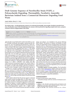
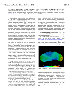
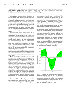
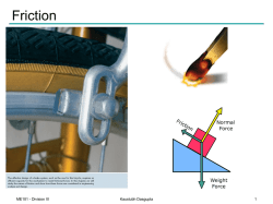
Three-Dimensional Discrete Element Simulations of Direct Shear Tests
Catherine O’Sullivan, Liang Cui
Department of Civil Engineering, University College Dublin, Ireland
Jonathan D. Bray
Department of Civil and Environmental Engineering, University of California, Berkeley, USA
ABSTRACT: Using discrete element simulations, one can monitor the micro-mechanisms driving the macroresponse of granular materials and quantify the evolution of local stress and strain values. However, it is
important to couple the se simulations with carefully controlled physical tests for validation and insight.
Only then can findings about the micro- mechanics of the material response be made with confidence. Moreover, the sensitivity of the observed response to the test boundary conditions can be analyzed in some detail.
The results of three-dimensional dis crete element simulations of direct shear tests and as well as complementary physical tests on specimens of steel balls are presented in this paper. Previous discrete element analyses
of the direct shear test have been restricted to two-dimensional simulations. For the simulations presented
here, an analysis of the internal stresses and contact forces illustrates the three-dimensional nature of the material response. The distribution of contact forces in the specimen at larger strain values, however, was
found to be qualitatively similar to the two-dimensional results of Zhang and Thornton (2002). Similarities
were also observed between the distrib ution of local strain values and the distribution of strains obtained by
Potts et al (1987) in a finite element analysis of the direct shear test. The simulation results indicated that
the material response is the stress dependent. However, the response observed in the simulations was found to
be significantly stiffer than that observed in the physical tests. The angle of internal friction for the simulations was also about 3o lower than that measured in the laboratory tests. Further laboratory tests and simulations are required to establish the source of the observed discrepancies.
1 INTRODUCTION
To date, much of our understanding of soil response has developed using standard laboratory
tests. Much can be learned by revisiting these tests
and examining the micro- mechanics underlying the
observed macro-scale response using discrete element method (DEM) analyses of these tests. This
paper presents some preliminary results of an ongoing analysis of the direct shear test that couples
physical tests and DEM simulations. The physical
tests on stainless steel spheres are described firstly.
Following a detailed description of the details of the
DEM simulation approach, the numerical results are
compared with the physical tests results. Significant differences in the material responses were observed. The next phase of this research will attempt to identify the source of these differences.
Analysis of the simulation results examined the local
stresses, the particle displacements, the contact
forces and the local strains. These results are co mpared with the earlier findings of Zhang and Thornton (2002) and Potts et al (1987).
2 BACKGROUND
Although there appears to be a slight difference
in opinion on the origin of the direct shear test, it is
unquestionably one of the oldest and most commonly used laboratory tests in geotechnical engineering. Holtz and Kovacs (1981) state that the
tests was originally used by Coulomb in the 18th
century, while Potts et al (1987) cite Skempton
(1949) who found that the test was first used in the
19th century by Alexandre Collin. In a preface to a
Geotechnique symposium in print on “The engineering application of direct and simple shear testing,”
Toolan (1987) observed that the direct shear test declined in popularity with the emergence of triaxial
testing. Toolan argues that testing with a direct
shear test provides essential data for applications
with low factors of safety where moderate displacements of the soil can be expected upon failure.
A recent publication by Lings and Dietz (2004) proposes modifications to the apparatus to facilitate
testing of sand, illustrating
continued interest in this apparatus. Other more recent research includes the experimental studies by
Shibuya et al (1997) and the finite element analyses
described by Dounias et al (1993) and Potts et al
(1987).
The standard test procedure for the direct shear
test is documented in ASTM D3080 (1990). Both
Potts et al (1987) and Shibuya et al (1997) note the
limitations of the test, including the non-uniformity
of the stresses and strain s induced in the soil and difficulties associated with interpreting the test results
to define a failure criterion. As noted by both Potts
et al and Shibuya et al, the popularity of the test can
largely be attributed to its simplicity.
Shibuya et al (1997) examined the influence of
boundary effects, such as wall friction, on the
specimen response. The distribution of normal and
shear stresses in the specimens tested were measured
using two-component load cells. Considering direct
shear tests on specimens of dense Toyoura sand the
effect of wall friction on the specimen response were
studied. It was found that as a result of wall friction, vertical stresses on the potential shear plane
were found to be substantially lower than the conventional measurement of vertical stress and that the
value of φ at peak was over-estimated when the
stress was calculated from the applied normal force
directly.
Potts et al (1987) and Dounias et al (1993) performed continuum-based numerical analyses of the
test using the finite element method. Potts et al
found that the reference stress state for the direct
shear box is that of simple shear. The study also
considered the influence of K0 on the specimen response. When a constitutive model without strain
softening was used to describe the material response,
the distribution of stresses and strains within the material were highly non-uniform. However when a
model incorporating significant strain softening was
used, the stresses and strains were more uniform.
Masson and Martinez (2001) used the twodimensional code PFC2D (Itasca, 2002) to simulate
two-dimensional direct shear tests using 1050 disks
of diameter 2, 3 and 4 mm. The particle scale responses analysed by Masson and Martinez included
the particle instantaneous velocity field, the distribution of particle horizontal and vertical displacements
as a function of depth and the distribution of particle
rotation as a function of depth. As other studies
have shown (e.g. Iwashita and Oda, 1998) the particle rotations were found to be a significant indicator
of strain localization. Masson and Martinez recognized the limitations of their two-dimensional study
and highlighted the potential sensitivity of their results to the particle-boundary friction value.
In another two-dimensional study, using a single
layer thickness of 5000 polydisperse spherical particles, Zhang and Thornton (2002) also analysed the
direct shear test using the TRUBAL code. Comparing the findings of Zhang and Thornton and Masson
and Martinez, the orientation of the contact forces at
the peak strength exhibit a more definite trend in the
simulation of Zhang and Thornton, most likely as a
consequence of the larger number of particles used.
All of these earlier studies of the direct shear test
using DEM considered two-dimensional analyses.
The work of Thomas (1997) quantitatively demonstrates the limitations of both two-dimensional DEM
simulations and physical tests using “Schneebli”
rods to represent real soil response. The current
study builds upon the findings of these earlier researchers by extending the simulations to three
dimensions.
Furthermore, by coupling the
numerical simulations with complementary physical
tests, further insight into the material response can
be obtained.
3 PHYSICAL TESTS
3.1 Direct shear testing
Some earlier research has explored the applicability of DEM to simulate the direct shear test. Mo rgan and Boettcher (1999) and Morgan (1999) used
the DEM code TRUBAL to simulate direct shear
tests with the objective of understanding the nature
of deformation of granular fault gouge. Morgan
and Boettcher calculated the directional derivative of
the horizontal displacement surface as a means to
highlight discontinuities in the specimen. They observed that at lower strain values (about 2%) the
deformation was broadly distributed across multiple
subhorizontal slip planes and progressively localized
onto a single shear plane by 8-10% strain.
A schematic diagram of the direct shear test apparatus used in the current study is given in Figure
1. The apparatus comprises a metal box of square
cross section (60 mm wide), divided in two halves
horizontally. The lower section of the box was
moved forward at a constant velocity (0.015 mm/s)
while the upper section of the box remained stationary. The force required to maintain the upper section of the box in a stationary position was measured
using a load cell and proving ring. The calibration
of the load cell was checked prior to testing. The
vertical load was applied to the top of the shear box
using a system of dead weights attached to a lever.
The test results are illustrated in Figure 2 and
summarized in Table 2. The shear stress was calculated by dividing the horizontal load measured in
the proving ring by the specimen cross sectional
area, while the vertical stress was calculated by dividing the applied vertical load by the specimen
cross-sectional area. As illustrated in Figure 2(b),
the friction angle φ for the material was found to be
24.4 o . However, as illustrated in both Figure 2(a)
and Figure 2(b), there was a degree of scatter in the
experimental results. By reference to Table 2 it can
be seen that the variation in specimen response appears to be largely a result of variation in the specimen void ratio values which were difficult to control
accurately.
Considering the maximum shear
stresses and the minimum shear stresses measured
for each normal stress, the maximum friction angle
was found to be 26.2o, while the minimum friction
angle was found to be 22.7o. To verify the experimental results the tests were repeated in the geotechnical laboratory at Trinity College Dublin. For
specimens with equivalent densities, the measured
friction angles differed by less than 0.25o.
Parameter
Radius
Density
Shear modulus
Poisson ratio
Friction coefficient*
Value
0.9922
7.8334 x 10-6
7.945 x 107
0.28
5.5 o
Unit
mm
kg/mm3
kg/(mm s 2)
Table 1: Material parameters of Grade 25 chrome steel balls
used in laboratory tests. *As determined by O’Sullivan (2002) for
equivalent balls
Load Cell
+ Proving Ring
60 mm
Actu ator
(Constant Velocity
= 0.015 mm/s)
21 mm
In the current study 0.9922 mm Grade 25 Chrome
Steel Balls were used (manufacturer: Thompson
Precision Ball). This material was used as the to lerances on the ball diameter and sphericity were
relatively tight (± 7.5 x 10-4 mm). The ball material properties are summarized in Table 1. The coefficient of friction values obtained by O’Sullivan
(2002) are used in the current study as the steel balls
used are equivalent to the steel balls considered in
the earlier study. For each test the balls were
placed in the shear box in three equal layers. Each
layer had a mass of 125 g (corresponding to 3900
balls). Following placement of the balls, five
“taps” of a hammer were applied to each vertical
side of the box to increase the specimen density.
Normal Force
Figure 1: Schematic diagram of direct shear test set-up
Test No.
Dense 1-1
Dense 1-2
Dense 1-3
Dense 2-1
Dense 2-2
Dense 2-3
Dense 3-1
Dense 3-2
Dense 3-3
Normal
Stress
(kPa)
54.5
54.5
54.5
109
109
109
163.5
163.5
163.5
Peak Shear
Stress (kPa)
Void Ratio
24.86
27.23
19.58
45.90
49.50
42.75
83.03
71.55
75.15
0.5841
0.5826
0.6089
0.5991
0.6097
0.5916
0.5818
0.6044
0.5969
Table 2: Summary of physical test results
4 DEM SIMULATIONS
4.1 Implementation of direct shear testing in
3DDEM
The distinct element method program (3DDEM)
used for the simulations described here is a modification of a code developed by Lin and Ng (1997) for
three-dimensional ellipsoidal particles, which in turn
is a modification of the Trubal DEM code (Cundall
and Strack, 1979). The program uses spherical particles and is further described in O’
Sullivan (2002).
In the DEM code, the Hertz-Mindlin contact model
is used to model the contact between spheres. Details of the implementation of this model can be
found in Itasca (2002) or Bardet (1998).
The method of simulating the direct shear test in
the 3DDEM code was originally proposed by
O’Sullivan (2002). A diagram illustrating the simulation procedure is given in Figure 3. During the
simulation, the specimen is enclosed by eight rigid
boundaries, two horizontal boundaries at the top and
bottom, two vertical boundaries at the front and
back, and four vertical boundaries at the left and
right of the specimen. Prior to shearing, the two left
boundaries are co-planar and the two right boundaries are co-planar. During shearing, one set of vertical boundaries is moved laterally with a constant velocity. An imaginary horizontal plane is constructed
through the middle of the specimen. All of the particles with centroids located above this plane are
checked for contact with the moving boundaries,
while all of the particles with centroids located below this plane are checked for contact with the stationary boundaries. Using this approach the comp utational cost associated with contact detection
between a sphere and the edge of the shear box is
avoided.
σ ij =
1
V
c=1
i
lic = xib − xia i, j = x, y, z
(2)
where xia and xib are the position vectors of the
spheres a and b meeting at contact c.
Prior to shearing the measurement sphere is used
in a servo-controlled system to bring the specimen
into a prescribed initial stress co nfiguration. If the
stress measured within the measurement sphere,
σ iimeas , differs from the user-specified stress, σ iireq ,
the boundaries perpendicular to i direction are
slowly moved so that the measured stress attains the
required stress values.
A servo-controlled approach is also used during the test so that the vertical stress, as measured in the measurement sphere,
remains constant during shearing.
A detailed
description of the implementation of the servo controlled system in 3DDEM is given by O’Sullivan
(2002).
Nc
∑f
branch vector connecting two contacted particle, a
and b. The branch vector is given by
c c
i
l
Moving
Boundaries
Shear Plane
Measurement
Sphere
To Control
σ zz
z
Stationary
Boundaries
y
Direction of Shearing
x
Figure 3: Illustration of implementation of direct shear tests in
code 3DDEM.
Figure 2: Summary of physical test results, (a) Shear stress versus horizontal strain (b) Shear stress versus normal stress
4.2
The measurement sphere illustrated in Figure 3 is
used to measure the average stresses in the specimen. Such a system to measure stress in discrete
element simulations has been described by a number
of researchers including Bardet (1998). The ave rage stress σ ij in the sphere is given by
σ ij =
1
V
Nc
∑f
i
c c
i
l
(i, j = x, y, z)
(1)
c= 1
where N c is the number of contacts within the
measurement sphere, V is the volume of the sphere,
f i c is the contact force at contact c, l ic is the
Analysis Parameters
Table 3 lists the input parameters used in the
simulation. A comparison of the parameters listed in
Table 3 and Table 1 illustrates that the physical test
and numerical simulation are equivalent, apart from
the differences in density value used.
Density
scaling is commonly used to reduce the computational cost associated with DEM simulations for
quasi-static analysed (e.g. Morgan and Boe ttcher
(1999), Thornton (2000), O’Sullivan et al (2004)).
The maximum stable time increment for explicit
DEM simulations is proportional to the square root
of the particle mass, motivating the use of such scaling. In the current analyses attempts were made to
run the simulations without any density scaling.
However, significant difficulties were encountered
in bringing the system into equilibrium. These
problems may have been a cons equence of the small
particle masses used in comparison with the contact
stiffnesses. Note that O’Sullivan (2002) performed
a detailed analysis of the sensitivity of simulations
of quasi- static triaxial tests to the input parameters.
The results of this analysis indicated that once the
ratio s σconfining/K and ρ /K remained constant there
was no variation in the simulation results (σ confining
=confining pressure, K=linear contact spring stiffness, ρ =particle density).
Previous analyses by O’Sullivan et al (2004) that
considered specimens with re gular packing configurations confirmed that these precision steel ball particles can be modelled using uniform spheres. While
some variation in the coefficient of friction values
for the particles was measured, such variation has a
negligible influence on the specimen response for
specimens with irregular packing configurations
(O’
Sullivan et al 2002). For the analyses discussed
in this paper the ball-boundary coefficient of friction
was assumed to be zero. In discrete element simulations of laboratory tests we can easily examine the
influence of boundary friction values on the macroscale response. Future analyses will explore this issue in more detail.
Parameter
Radius
Density
Shear modulus
Poisson ratio
Friction coefficient
Value
0.9922
7.8334 x 103
7.945 x 107
0.28
Unit
mm
kg/mm3
kg/(mm s 2)
mathematicians to develop algorithms to generate
dense, random assemblies of spheres (e.g. Zong
(1999)). For the current analysis one such algorithm, proposed by Jodrey and Tory (1985), was initially used to generate the spec imen. The resultant
specimen was however less dense than the specimens tested in the lab (with a void ratio of 0.77 in
comparison to void ratios of 0.58 – 0.61). To overcome this limitation and achieve the required density
value, 11700 balls with a radius of 0.9393 mm
were initially gene rated in a box of size 0.06 x 0.06
x 0.02 mm. This radius was then gradually expanded
to 0.9922 mm, the box height was increased to 21
mm, and a DEM simulation was run until the system
came into equilibrium. During this simulation the
inter-particle friction angle was assigned a value of
zero. The behavior of the particles during the equilibrium phase can be understood by reference to
Figure 4. Initially upon initial radius expansion
there was significant inter-particle overlap, with a
maximum particle overlap of approximately 0.1059
mm (Figure 4(a)). As the equilibrium phase of the
analysis progressed the balls moved to assume a
dense packing configuration with a minimum
amount of particle overlap (Figure 4(c)). Prior to
shearing the maximum overlap was approximately
1.73 x 10-3 mm.
4.4
Direct Shear Test Simulations
4.3 Specimen generation
Three DEM simulations were performed with initial isotropic stress conditions of 54.5 kPa, 109 kPa
and 163.5 kPa. These initial stress conditions were
attained using the servo-controlled approach detailed
above. The upper section of the box was moved at a
velocity of 0.001 mm/sec. It is important in these
servo-controlled tests to verify firstly that the specified stress conditions are maintained for the duration
of the simulation. A period of initial iteration was
required to determine the appropriate control parameters to meet this requirement. Figure 5 illustrates the vertical stress in the specimen during the
simulations as a function of horizontal strain. Both
the vertical stress measured in the measurement
sphere as well as the vertical stress calculated from
the measured boundary forces are illustrated. The
measured stresses varied slightly during the simulations, with a maximum deviation of 5% from the
specified value measured in the measurement
sphere.
The difficulties associated with generating a
three-dimensional specimen to a specific void ratio
for use in a discrete element analysis cannot be
overstated. A review of some of the available approaches to specimen generation is provided by Cui
and O’Sullivan (2003). As noted by O’Sullivan
(2002), considerable effo rt has been expended by
The macro-scale test results are summarized in
Table 4 and Figure 6. Figure 6(a) is a plot of shear
stress versus hor izontal strain, and Figure 6(b) is a
plot of peak shear stress versus normal stress. The
results yield a value for the angle of internal friction
of 19.6 o , which compares with a value of 22.7o as
the minimum value obtained in the laboratory tests.
5.5 o
Table 3: Input parameters for DEM simulations
(a)
(b)
(c)
Figure 4: Illustration of specimen generation phase of analysis
The void ratios of the specimens in the DEM simulations were close to the minimum void ratio values
of the test specimens. Hence, the DEM simulations
were found to underestimate the strength of the ball
assembly measured in the laboratory.
Required Vertical Stress 163 kPa (Meas. Sphere)
Required Vertical Stress 109 kPa (Meas. Sphere)
Required Vertical Stress 54 kPa (Meas. Sphere)
Required Vertical Stress 163 kPa (Boundary Force)
Required Vertical Stress 109 kPa (Boundary Force)
Required Vertical Stress 54.5 kPa (Boundary Force)
analyses will explore the influence of ball-boundary
friction on the macro-scale response as well as the
contact constitutive model used in the simulations.
Coupling physical tests and numerical simulations is non-trivial as it can be difficult to replicate
the exact details of the physical test in the numerical
simulation. O’
Sullivan (2002) describes some of
the challenges associated with successful validation
of discrete element codes using physical tests.
Vertical Stress 163 kPa (DEM)
Vertical Stress 109 kPa (DEM)
Vertical Stress 54.5 kPa (DEM)
160
80
120
Shear Stresses (KPa)
Normal Stress (KPa)
200
80
40
0
0
0.01
0.02
0.03
0.04
0.05
0.06
Horizontal Strain
60
40
20
0
-20
Figure 5: Normal Stresses (σzz) as calculated for measurement
sphere and vertical stresses calculated from boundary forces
for the three simulations considered.
0
0.02
0.04
0.06
Horizontal Strain
(a)
Test No.
1
2
3
Normal
Stress, kPa
54.5
109
163.5
Peak Shear
Stress, kPa
15.9
37.5
60.4
Void Ratio
0.587
0.587
0.587
Table 4: Summary of test simulation results.
A comparison of Figure 2 and Figure 6 indicates
that the numerical simulations exhibit a significantly
stiffer response in comparison to the physical tests.
Considering the volumetric strain response of the
physical test specimens, some compression was observed at the start of shearing prior to dilation.
However for the numerical simulations the specimens dilated from the onset of shearing. These
differences in volumetric strain response, suggest
that there may be significant differences between the
fabric of the physical test specimens and the fabric
of the specimens analyzed using DEM. In physical
tests, O’
Sullivan (2002) observed that the response
of specimens of uniform steel balls is very sensitive
to the specimen preparation approach; specimens
with similar void ratios can exhibit different responses depending upon the specimen preparation
approach used. Future research will address the
source of these discrepancies considering the sens itivity of the response to the specimen preparation
method as well as any compliance of the laboratory
apparatus. As a quality assurance procedure the
tests will be replicated using an alternative direct
shear box located in another laboratory. Further
Peak Shear Stress (kPa)
100
Test Data
DEM simulations
80
φDEM = 19.6 o
60
40
20
0
0
40
80
120
160
200
Normal Stress (kPa)
(b)
Figure 6: Su mmary of DEM simulation results. (a) Shear stress
versus horizontal strain. (b) Peak shear stress versus normal
stress
Notwit hstanding the discrepancies between the
stiffness observed in the laboratory tests and the
numerical simulations, the numerical simulations
clearly captured some of the typ ical response characteristics of granular materials in direct shear tests.
For example, the stress-dependency of the specimen
response can clearly be seen with the ratio of the
peak shear stress to the residual shear stress increasing as the normal stress increases. Such stress dependency, however, was not observed in the physical tests. It is also interesting to observe in Figure
6(a) that the three specimens tested in the direct
shear test appear to approach a similar value of shear
stress (about 20kPa) as shearing progresses to large
displacements.
d
5 ANALYSIS OF MICRO -SCALE
PARAMETERS
H
5.1 Stress analysis
z
y
Di rection of S hearing
x
Figure 7: Illustration of configuration of rectangular box used
to calculate local stresses
50
Shear Stress from Boundary Forces
σ zx , d=2/5H
σzx , d=1/5H
σzx , d=1/10H
Shear St resses (KPa)
40
Vertical stress = 54.5 kPa
30
20
10
0
0
0.02
0.04
0.06
Horizontal Strain
(a)
50
Vertical stress = 109 kPa
40
Shear Stresses ( KPa)
In a direct shear test the shear stress along the region of localization is inferred from the macro-scale
measurement of shear force. In the DEM analyses
a series of rectangular boxes were created and the
average stresses within this box were calculated using Equation 1. The configuration of these boxes is
illustrated in Figure 7; the center of the stress measurement box was located at the center of the specimen and the thickness of the box, d, ranged from
H/10 to 2H/5, where H is the specimen height. The
variation of the local stresses, σ xz , as measured in
the stress measurement box, with increasing strain is
illustrated in Figure 8.
30
20
As illustrated in both Figure 8(a) and Figure 8(b),
the shear stress, σ zx , measured increased as the
thickness of the measurement box decreased. For
an applied vertical stress of 54 kPa (Figure 8(a)), the
σzx values consistently exceeded the global shear
stress values (calculated from the boundary forces).
However, for an applied vertical stress of 109 kPa
(Figure 8(b)) and an applied vertical stress of 163
kPa (not shown), the local shear stress (σ zx ) values
were less than the global shear stress. For the three
vertical stresses considered, the ratio of the peak σzx
value for d=1/5 H divided by the peak σzx value for
d=2/5 H is consistently 1.1, whereas the ratio of the
peak σzx value for d=1/10 H divided by the peak σzx
value for d=2/5 H is consistently 1.3.
5.2 Incremental Displacements
Shear Stress from Boundary Forces
σzx , d=2/5H
σzx , d=1/5H
σ , d=1/10H
10
zx
0
0
0.01
0.02
0.03
0.04
0.05
Horizontal Strain
(b)
Figure 8: Variation of shear stress (σzx) values, measured in
measurement boxes, as a function of horizontal strain. (a) Vertical stress = 54.5 kPa. (b) Vertical stress = 109 kPa.
A three-dimensional plot of the incremental displacements for the simulation with a normal stress of
54kPa is illustrated in Figure 9 for the horizontal
strain increment 0.003 to 0.052. Figure 9(a) is a
front view of the specimen and Figure 9(b) is a side
view of the specimen. For ease of visualization
only displacements exceeding the average incremental displacement are illustrated.
Referring
firstly to Figure 9(a), as would be expected, most of
the displacement is concentrated in the upper half of
the shear box. There also is a concentration of displacement vectors close to the left and right boundaries. At the left hand side of the box there is significant downward motion of the particles. The
magnitude of the upward displacement of the particles in the upper right section of the box is less than
the magnitude of the downward motion of the parti-
cles close to the left boundary. Comparing Figure
9(a) and Figure 9(b), it is clear that the components
of the particle displacement vectors in the ydirection are small in comparison to the component
of the vectors in the z-direction.
shear test. The forces are transmitted diagonally
across the specimen. An orthogonal view of the
specimen, along the z axis, is given in Figure 10(b),
however, it is difficult to identify any clear trend in
the orientation of the contact force vectors from this
perspective.
5mm
1N
z
z
x
x
(a)
(a)
5mm
1N
z
z
y
y
(b)
Figure 9: Incremental displacement vectors for horizontal
strain increment of 0.003 to 0.052, vertical stress 54.5 kPa.
(a) Front view (looking along y axis) (b) Side view (looking
along x axis). Note: For ease of visualization only displacements exceeding the mean displacement value are illustrated.
5.3 Contact forces
In order to appreciate the spatial variation in the
contact forces, a three-dimensional plot of the unit
contact force vectors for the simulation with a no rmal stress of 54kPa at a horizontal strain of 0.052 is
illustrated in Figure 10. Figure 10(a) is a front
view of the specimen and Figure 10(b) is a side view
of the specimen. For ease of visualisation, only
contacts where the magnitude of the contact force
exceeds the average contact force + 1 standard deviation are considered. The distribution of contact
forces illustrated in Figure 10(a) is qualitatively
similar to the distribution of contact forces obtained
by Zhang and Thornton (2002) in their twodimensional discrete element analysis of the direct
(b)
Figure 10: Contact force vectors at a horizontal strain of
0.052, vertical stress 54.5 kPa.
(a) Front view (looking
along y axis) (b) Side view (looking along x axis). Note: For
ease of visualization only contacts where the forces exceeds the
average contact force + 1 standard deviation are considered.
Figure 11 is a three dimensional plot of the contact force vectors, giving an indication of both the
magnitude and direction of the contact forces. As
illustrated in Figure 11(a) it is clear that the xcomponent of the contact force exceeds the zcomponent. Considering the distribution of the y
and z components of the contact forces, the plot is
approximately circular, as illustrated in Figure 11(b).
The y and z components of the contact forces are
therefore relatively evenly distributed. An analysis
of the local normal stresses as calculated from the
contact forces indicated that σ xx >σ yy >σzz. The
relatively large value in σ yy is an indicator of the
three dimensional nature of the problem.
scribed by O’Sullivan and Bray (2003) where a distinct localization was observed in three-dimensional
simulations of plane strain tests.
0.5 N
γ xy
0
z
0.25
x
γ yz
(a)
0.5
0
0.25
0.5N
γ zx
0.5
0
0.25
εvol
0.5
0
z
y
0.25
(b)
0.5
Figure 11: Three dimensional plot of contact force vectors
(a) Front view (looking along y axis) (b) Side view (looking
along x axis).
5.4 Strain localization analysis
For the simulation with a vertical stress of 163 kPa,
the local strain values were calculated using the nonlinear homogenization technique proposed by
O’Sullivan et al (2003). The strain values are plo tted on a vertical plane through the center of the
specimen, i.e. with y=30 mm. Figure 12 illustrates
the local strain values for the horizontal strain increment from 0.003 to 0.017. While there are
zones with high strain va lues at mid height close to
the left and right boundaries, no clear localization
through the center of the specimen is apparent, even
though the specimen is close to the peak stress at
this strain level.
Considering the volumetric
strain values (ε vol), the localizations appear to be inclined. Similar inclined localizations were observed by Potts et al (1987) where a constitutive
model without strain softening was used.
Figure 13 illustrates the distribution in strain va lues at a horizontal strain of 0.047. The distrib ution
of shear strains is highly irregular and there is still
no clear evidence of a localization in the specimen.
Similar strain distributions were observed for the
specimens with vertical stresses of 54.5 kPa and 109
kPa. This contrasts with the study of localizations
in specimens with regular packing configuration de-
Inclined localizations
Figure 12: Strain contours for horizontal strain increment 0.003
to 0.017, plotted on a vertical plane through center of specimen
with y=30. Normal stress 163 kPa. Contour interval 0.025.
6 DISCUSSION
The direct shear test has been studied using discrete element analysis in combination with a series
of complementary physical tests. The agreement
between the laboratory tests and the numerical simulations was not wholly satisfactory. The angle of
friction calculated using the results of the simulations was 3o lower than that obtained in the physical
tests. The response in the simulations was also
stiffer than the response observed in the physical
tests. Further tests and simulations are required to
resolve these discrepancies, although it is likely that
test device friction may be a contributing factor.
An analysis of the results of the simulations considered the local stress values, the incremental displacements, the distribution of contact forces and the
local strain values. Whereas the particle displacements were predominantly restricted to the direction
of shearing (i.e. parallel to the y=0 plane), significant contact forces developed in the y-direction, illustrating the three dimensional nature of the material response at the particle scale. Within the
specimen, the stresses are non- uniform with the
shear stresses increasing closer to the zone of shearing. The local strain values are non- uniform and the
localization cannot be identified at horizontal strains
of approximately 5%.
γx y
0
0.5
γy z
1
0
0.5
γz x
1
0
0.5
ε vol
1
0
0.5
1
Figure 13: Strain contours for horizontal strain increment 0.003
to 0.047, plotted on a vertical plane through center of specimen with y=30. Normal stress 163 kPa. Contour interval 0.05.
ACKNOWLEDGEMENTS
Funding for this research was provided by the Irish
Research Council for Science, Engineering and Technology (IRCSET) under the Basic Research Grant Scheme.
Additional partial funding was provided by the Institution
of Engineers of Ireland Geotechnical Trust Fund. The
authors are grateful to Mr. George Cosgrave, University
College Dublin, for his assistance in performing the laboratory tests.
REFERENCES
ASTM (1990) D3080: standard test method for direct shear test
of soils under consolidated drained conditions, Annual book
of ASTM standards: 417-422
Cui, L. and C. O’Sullivan (2003)
“
Analysis of a Triangulation Based Approach for Specimen Generation for Discrete Element Simulations.” Granular Matter V.5(3): 135145
Dounias, G.T. and Potts, D.M. (1993) “Numerical analysis of
drained direct and simple shear test” Journal of Geotechnical Engineering Vol. 119, No. 12, 1870-1891
Holtz R. D. and Kovacs, W.D. (1981) An Introduction to Geotechnical Engineering Prentice Hall.
Itasca (2002). PFC2D Manual, Theory and Backround.
Iwashita, K. and Oda, M., “Micro-deformation mechanism of
shear banding process based on modified distinct element
method”, Powder Technology 109: 192-205 (2000).
Jodrey, W.S. and Tory, E.M. (1985) “Computer simulation of
close random packing of equal spheres” Physical Review A
32 (4): 2347-2351
Lings, M.L. and Dietz, M.S. (2004) “An improved direct shear
apparatus for sand”Geotechnqiue Vol. 54 No. 4 245-256
Masson, S. and Martinez, J. (2001) “Micromechanical analysis
of the shear behavior of a granular material” ASCE Journal
of Engineering Mechanics, Vol. 127, No. 10: 1007-1016
Morgan, J. and Boettcher, M.S. (1999) “Numerical simulations
of granular shear zones using the distinct element method.
1. Shear zone kinematics and the micromechanics of loca lization” Journal of Geophysical Research, Vol. 104, No.
B2: 2703-2719
Morgan, J. (1999) “Numerical simulations of granular shear
zones using the distinct element method. 2. Effects of part icle size distribution and interparticle friction on mechanical
behavior”Journal of Geophysical Research, Vol. 104, No.
B2: 2721-2732
O’Sullivan, C. (2002). The Application of Discrete Element
Modelling to Finite Deformation Problems in Geomechanics. Ph.D. thesis, Dept. of Civ. Engrg., Univ. of California,
Berkeley.
O'Sullivan, C., J.D. Bray, and M.F. Riemer, (2002) “
The Influence of Particle Shape and Surface Friction Variability
on Macroscopic Frictional Strength of Rod-Shaped Particulate Media” ASCE Journal of Engineering Mechanics, Vol.
128, No. 11. p 1182-1192
O'Sullivan, C. and J.D. Bray (2003) “Evolution of Localizations in Idealized Granular Materials” Workshop on Quasistatic Deformations of
Particulate Materials
O'Sullivan, C., Bray, J.D. and M.F. Riemer, (2004) “An examination of the response of regularly packed specimens of
spherical particles using physical tests and discrete element
simulations.” ASCE Journal of Engineering Mechanics,
Vol. 130, No. 10, in press.
O’Sullivan, C., Bray, J. D. and Li, S. (2003) “A New Approach for Calculating Strain for Particulate Media” International Journal for Numerical and Analytical Methods in
Geomechanics Vol. 27 No. 10.: 859-877.
Potts, D. M., Dounias, G.T., and Vaughan, P. R. (1987) “Finite
element analysis of the direct shear box test”Geotechnique,
Vol. 37, No. 1: 11-23
Skempton, A. W. (1949) Alexandre Collin: a note on his pioneer work in soil mechanics, Geotechnique, Vol. 19., No. 1:
75-86
Thomas, P.A. (1997) Discontinuous deformation analysis of
particulate media. Ph.D. thesis, Dept. of Civ. Engrg., Univ.
of California, Berkeley.
Toolan, F.E. (1987) Preface to “Syposium in print on the engineering application of direct and simple shear testing”,
Geotechnique 1987, Vol. 37, No. 1, 1-2.
Shibuya, S., Mitachi, T., and Tamate, S. (1997) “Interpretaion
of direct shear box testing of sands as quasi-simple shear”
Geotechnique 47(4): 769-790
Zhang, L and Thornton, C. (2002a). “DEM simulations of the
direct shear test”. Proceedings of 15 th ASCE Engineering
Mechanics Conference, June2-5, 2002. Columbia University, New York, NY.
Zong, C. (1999) Sphere Packings, Springer.