1. Art and Diseño

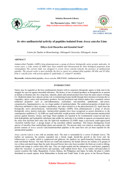
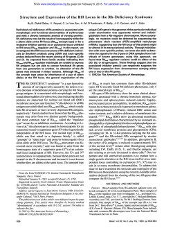
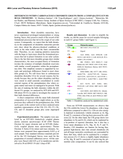
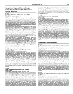
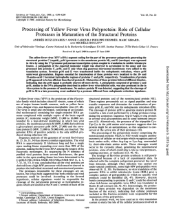
Li et al. Clinical Proteomics 2015, 12:3
http://www.clinicalproteomicsjournal.com/content/12/1/3
RESEARCH
CLINICAL
PROTEOMICS
Open Access
An integrated quantification method to increase
the precision, robustness, and resolution of
protein measurement in human plasma samples
Xiao-jun Li1*, Lik Wee Lee1, Clive Hayward1, Mi-Youn Brusniak1,2, Pui-Yee Fong1, Matthew McLean1,3,
JoAnne Mulligan1, Douglas Spicer1, Kenneth C Fang1, Stephen W Hunsucker1 and Paul Kearney1
Abstract
Background: Current quantification methods for mass spectrometry (MS)-based proteomics either do not provide
sufficient control of variability or are difficult to implement for routine clinical testing.
Results: We present here an integrated quantification (InteQuan) method that better controls pre-analytical and
analytical variability than the popular quantification method using stable isotope-labeled standard peptides
(SISQuan). We quantified 16 lung cancer biomarker candidates in human plasma samples in three assessment
studies, using immunoaffinity depletion coupled with multiple reaction monitoring (MRM) MS. InteQuan
outperformed SISQuan in precision in all three studies and tolerated a two-fold difference in sample loading.
The three studies lasted over six months and encountered major changes in experimental settings. Nevertheless,
plasma proteins in low ng/ml to low μg/ml concentrations were measured with a median technical coefficient of
variation (CV) of 11.9% using InteQuan. The corresponding median CV using SISQuan was 15.3% after linear fitting.
Furthermore, InteQuan surpassed SISQuan in measuring biological difference among clinical samples and in
distinguishing benign versus cancer plasma samples.
Conclusions: We demonstrated that InteQuan is a simple yet robust quantification method for MS-based
quantitative proteomics, especially for applications in biomarker research and in routine clinical testing.
Keywords: Multiple reaction monitoring, Plasma or serum analysis, Quantitative proteomics, Clinical proteomics,
Mass spectrometry, Immunoaffinity depletion, Bioinformatics
Background
Multiple reaction monitoring (MRM, also known as selected reaction monitoring) mass spectrometry (MS)
allows for the fast and reproducible measurement of tens
to hundreds of proteins in complex biological samples
such as bio-fluids, tissues, and cultured cells [1-5]. There
is tremendous interest in applying the technology to develop blood-based clinical tests for the diagnosis, prognosis or treatment stratification of various diseases [6-9].
Due to the high complexity of the human blood proteome
[10], proteomic analysis of blood samples (that is serum or
plasma) typically consists of multiple experimental steps
* Correspondence: [email protected]
1
Integrated Diagnostics, 219 Terry Avenue North, Suite 100, 98109 Seattle,
WA, USA
Full list of author information is available at the end of the article
and is prone to variation [1,11] (Figure 1A). In addition,
changes in laboratory conditions (e.g., operators, instruments, reagents) are expected during routine laboratory
operations in clinical testing. Therefore, controlling analytical variability to satisfy rigorous quality control requirements for blood-based clinical testing using MRM-MS
platforms has been challenging.
The principle of stable isotope labeling (SIL) is widely
used in MS-based quantitative proteomics to control
experimental variability [12-18]. Protein abundance is
measured by comparing MS signal intensities of endogenous peptides with those of their corresponding
stable isotope-labeled internal standard (SIS) peptides.
Three SIL approaches are potentially suitable for clinical
testing (Figure 1B). The first approach utilizes SIS peptides for protein quantification [12,13] (SISQuan) and is
© 2015 Li et al.; licensee BioMed Central. This is an Open Access article distributed under the terms of the Creative Commons
Attribution License (http://creativecommons.org/licenses/by/4.0), which permits unrestricted use, distribution, and
reproduction in any medium, provided the original work is properly credited. The Creative Commons Public Domain
Dedication waiver (http://creativecommons.org/publicdomain/zero/1.0/) applies to the data made available in this article,
unless otherwise stated.
Li et al. Clinical Proteomics 2015, 12:3
http://www.clinicalproteomicsjournal.com/content/12/1/3
A
Procedure
Sources of systematic
variation
Difference in sample
collection affecting total
protein concentration
Sources of proteinspecific variation
Difference in sample
shipment affecting protein
degradation
Sources of peptidespecific variation
-
Depletion
Pipetting error affecting
loading volume
Column aging affecting
protein affinity
-
Digestion
Difference in trypsin
activity and/or
concentration
Difference in digestion
efficiency due to protein
structure
Difference in over- or
under-digestion due to
peptide sequence
Desalting
Pipetting error, difference
in reagent purity and/or
concentration
-
Difference in peptide
recovery rate
Difference in instrument
sensitivity
-
Difference in peptide
retention time and/or ion
suppression
Pre-analytical
MS analysis
B
Page 2 of 17
Procedure
SIS
peptides
Full-length
SIS proteins
Artificial or
truncated
SIS proteins
Endogenous
proteins
Integrated
quantification
Pre-analytical
Depletion
Digestion
Desalting
MS analysis
Types of variation under control:
Systematic, protein- and/or peptide-specific
Systematic and peptide-specific
Systematic
None
C
Study
Assessment
Sample types
Study I
Precision on HPS when
a large number of
samples were depleted
using a single column.
60 clinical samples,
12 aliquots of HPS.
Study II
Control on analytical
variation when clinical
samples were depleted
using multiple columns.
Study III
Combined
HPS
dataset
Total
samples
72
Total
depletion
columns
1
Loading
volume per
sample ( l)
30
18 clinical samples
(each in triplicate), 12
aliquots of HPS.
66
3
20
Tolerance against
variation in the total
protein concentration in
clinical samples.
6 samples (each in
duplicate and in three
concentrations), 8
aliquots of HPS.
44
2
30, 20, or 15
Robustness of
depletion-MRM-MS
platform.
32 aliquots of HPS
across all three
studies.
32
(HPS: 30)
6
30 or 20
Figure 1 Overview of experimental variations and control methods. (A) Exemplar sources of variations. Systematic variations affect all
proteins or peptides similarly. Protein- or peptide-specific variations affect only particular proteins or peptides. Random variations are not listed
because they are not controllable. (B) Control of variations by different quantification methods in the analysis of plasma samples on a
depletion-MRM-MS platform. (C) Overview of the three assessment studies and the combined HPS dataset.
the simplest one for implementation. SIS peptides are
synthesized, optimized for MS analysis and spiked into
samples before [12] or after [13] protein digestion to
control variation in post-digestion procedures. However,
variation occurring before or during digestion is not
controlled. The second approach [14-16] spikes fulllength SIS proteins into samples before any analytical
procedure takes place. While this approach offers the
Li et al. Clinical Proteomics 2015, 12:3
http://www.clinicalproteomicsjournal.com/content/12/1/3
best control of analytical variability, it is applicable only
to soluble proteins. Quality control of the production,
the storage, etc., of SIS proteins as standards is challenging for routine laboratory operations [14]. The third approach spikes either artificial [17] or truncated [18] SIS
proteins into samples before protein digestion. It controls most variation in protein digestion and variation in
subsequent procedures. However, it cannot control variation occurring before digestion and faces similar implementation challenges as the second approach. None of
the above SIL approaches can control pre-analytical variability associated with sample collection and handling. A
simple and robust method that provides sufficient control of pre-analytical and analytical variability for routine
clinical testing on MS-based proteomics platforms is
still lacking.
We recently analyzed hundreds of human plasma samples in a discovery study of lung cancer biomarkers [6],
using immunoaffinity-based protein depletion coupled
with MRM-MS (depletion-MRM-MS). In the study we
identified six endogenous normalizing proteins from 371
protein candidates. Since the normalizing proteins were
processed and analyzed together with target proteins of
interest, we expected them to serve as monitors for systematic variation in both pre-analytical and analytical
procedures (Figure 1B). We verified that experimental
variability was reduced after normalization by a panel of
the six proteins. Although this method of endogenous
protein normalization (EPN) and similar approaches
have been reported previously in quantitative proteomics
[7,19-22], our approach is unique. The six normalizing
proteins were selected by their ability to compensate
both the drift of depletion columns and the technical
variation of other proteins [6], rather than their ‘housekeeping” properties as utilized in other approaches.
However, the EPN quantification method used in our previous study is a label-free approach and cannot control analytical variability as narrowly as the three SIL approaches.
Since our label-free discovery study [6], we have developed more accurate MRM assays for target proteins of
interest [23], using the SIL approach of SIS peptides. As
reviewed above, neither SIL nor EPN is ideal for protein
quantification in clinical proteomics. To deal with this
challenge, we present here a new quantification method,
named integrated quantification (InteQuan), to combine
the advantageous features of the two methods: The
six endogenous normalizing proteins were used to compensate systematic variation in pre-analytical procedures
and in depletion and digestion; SIS peptides were
used to control variation in desalting and MS analysis
(Figure 1B). To mimic an actual clinical testing scenario,
we completely defined details of InteQuan method based
on data from a different study [23] before assessing its
performance in three independent studies (Figure 1C).
Page 3 of 17
To the best of our knowledge, no one has described
such a method to quantify individual proteins before. A
recent work used “sparse reference labeling” to anchor
protein abundance that can be valuable for biomarker
discovery [24]. Nevertheless, individual proteins were essentially quantified in a label-free approach in the study,
leaving peptide-specific variation in MS analysis uncontrolled and thus reducing its validity for routine clinical
testing. In this study we demonstrated that InteQuan increased the precision, robustness, and resolution of protein measurement in the three independent assessment
studies.
Results and discussion
Protein quantification in human plasma samples
A total of 21 lung cancer biomarker candidates were
identified in our recent discovery study [6]. Two of the
21 candidates (GSLG1 and EF1A1) were eliminated from
this study due to weak signals on a new MRM-MS platform. Another candidate (FIBA) was eliminated due to
its affinity to the depletion column [25]. The remaining
18 candidates (Table 1) were targeted for quantification
in human plasma samples.
Six endogenous normalizing proteins (Table 1) were
selected from a pool of 371 protein candidates in our
previous label-free discovery study [6]. The predicted
plasma concentration [26] of the six proteins, estimated
from the occurrence of protein detection in human
plasma or serum samples by the proteomics community,
ranged from 9.9 ng/ml (PTPRJ) to 16 μg/ml (GELS). All
six proteins were used as normalizing proteins for InteQuan and for EPN in this study.
Human plasma samples were analyzed on a depletionMRM-MS platform. SIS peptides of the target and the
normalizing proteins were synthesized and spiked into
peptide samples after digestion. The specificity of MRM
assays to the corresponding proteins was verified for all
proteins except for LRP1 and AIFM1. As shown in
Additional file 1: Figure S1, MRM signals of verified assays were well above the corresponding noise level; endogenous and SIS peptides co-eluted and had comparable
intensity ratios between different transitions. The highest
false discovery rate (FDR) of the original assays was 0.44%
(ISLR, see Table 1). As shown later in Study III, proteins
were also measured within the respective linear dynamic
range of the assays. Two blank samples were processed
and analyzed at the end of each experimental batch in
Study II and III to monitor possible carryover from previous samples (see Additional file 2: Table S1). MRM signals in those blank samples were just above noise level
(data not shown), indicating that carryover was not a
problem for the depletion-MRM-MS platform. After validating the MRM assays, LRP1 and AIFM1 were both
eliminated from further analysis. The predicted plasma
Li et al. Clinical Proteomics 2015, 12:3
http://www.clinicalproteomicsjournal.com/content/12/1/3
Page 4 of 17
Table 1 List of six normalizing proteins and eighteen target proteins of interest
Protein
(HUMAN)
Protein name
Concentrationa
(ng/ml)
Transitionb (peptide_Q1_Q3)
FDRc
Fn
d
⌣
Rn
e
Ăn f
Normalizing proteins
PEDF
Pigment epithelium-derived factor
7200
LQSLFDSPDFSK_692.34_593.30
1.40E-04 0.971
1.756
1.209E06
MASP1
Mannan-binding lectin serine protease 1
240
TGVITSPDFPNPYPK_816.92_258.10
5.75E-04 0.957
0.360
1.060E05
GELS
Gelsolin
16000
TASDFITK_441.73_710.40
3.18E-04 0.852
0.502
1.897E06
LUM
Lumican
4000
SLEDLQLTHNK_433.23_499.30
C163A
Scavenger receptor cysteine-rich type 1
protein M130
94
INPASLDK_429.24_630.30
1.19E-03 0.823
0.392
4.690E04
PTPRJ
Receptor-type tyrosine-protein
phosphatase eta
9.9
VITEPIPVSDLR_669.89_896.50
1.44E-03 0.926
0.275
4.685E04
ELWFSDDPNVTK_725.85_558.30
3.82E-04 0.838 10.846 4.717E06
Target proteins of interest
AIFM1
Apoptosis-inducing factor 1, mitochondrial
1.4
3.70E-02
Assay specificity
not verified
KIT
Mast/stem cell growth factor receptor
8.2
YVSELHLTR_373.21_428.30
2.40E-03 0.730
FRIL
Ferritin light chain
12
LGGPEAGLGEYLFER_804.40_1083.60
4.30E-05 0.844
LRP1
Prolow-density lipoprotein
receptor-related protein 1
20
COIA1
Collagen alpha-1(XVIII) chain
35
AVGLAGTFR_446.26_721.40
PRDX1
Peroxiredoxin-1
60
QITVNDLPVGR_606.30_970.50
1.90E-05 1.714
TENX
Tenascin-X
70
YEVTVVSVR_526.29_293.10
1.10E-03 0.699
TVLWPNGLSLDIPAGR_855.00_1209.70 1.40E-04
Assay specificity
not verified
6.70E-04 0.732
ENPL
Endoplasmin
88
SGYLLPDTK_497.27_308.10
1.10E-03 0.649
GRP78
78 kDa glucose-regulated protein
100
TWNDPSVQQDIK_715.85_288.10
1.80E-03 1.140
BGH3
Transforming growth factor-beta-induced
protein ig-h3
140
LTLLAPLNSVFK_658.40_804.50
1.40E-04 0.779
ALDOA
Fructose-bisphosphate aldolase A
250
ALQASALK_401.25_617.40
3.70E-05 0.777
GGH
Gamma-glutamyl hydrolase
250
YYIAASYVK_539.28_638.40
1.70E-03 0.834
CD14
Monocyte differentiation antigen CD14
420
ATVNPSAPR_456.80_527.30
4.30E-04 0.789
LG3BP
Galectin-3-binding protein
440
VEIFYR_413.73_598.30
2.80E-05 0.842
TSP1
Thrombospondin-1
510
GFLLLASLR_495.31_559.40
1.90E-05 0.625
IBP3
Insulin-like growth factor-binding
protein 3
5700
FLNVLSPR_473.28_685.40
2.80E-05 0.790
TETN
Tetranectin
58000
LDTLAQEVALLK_657.39_871.50
3.70E-05 0.760
ISLR
Immunoglobulin superfamily
containing leucine-rich repeat protein
ALPGTPVASSQPR_640.85_841.50
4.40E-03 0.850
a
Predicted plasma concentration [26]. bThe transition that was used for quantification. cFalse discovery rate for peptide MRM assay (peptide Q value) [6].
Correction factor {Fn} in Study II in which a new lot of SIS peptides were used. eScaling constant fŘn g for InteQuan. fScaling constant {Ăn} for EPN
d
concentration [26] of the 16 remaining target proteins
spanned four orders of magnitude from 8.2 ng/ml (KIT) to
58 μg/ml (TETN).
The target proteins were quantified based on MRM-MS
data using four different methods (raw MS data, EPN, SISQuan and InteQuan). In this study, the abundance of a
protein was evaluated based on the MRM signal intensity
of the strongest transition from the protein, as previously
justified [2,6]. Thus, no distinction was made between protein abundance, peptide abundance and transition abundance. For raw MS data, protein abundance was measured
by the peak area of the strongest transition of the protein.
For EPN, protein abundance using the raw MS data was
divided by a sample-dependent normalization factor that
was calculated from the peak areas of the six normalizing
proteins. Six scaling constants, one for each of the six
normalizing proteins, were used in the calculation of the
normalization factor. For SISQuan, protein abundance
was measured by the response ratio between the peak area
of the strongest transition of the target protein and the
peak area of the matching transition of the corresponding
SIS peptide. For InteQuan, protein abundance using SISQuan was divided by a sample-dependent normalization
factor that was calculated from the response ratios of
Li et al. Clinical Proteomics 2015, 12:3
http://www.clinicalproteomicsjournal.com/content/12/1/3
the six normalizing proteins. As with EPN, six scaling constants were used in the calculation of the normalization factor. In the study, we mainly focused on comparing the new
InteQuan method with the widely used SISQuan method.
All scaling constants for InteQuan and for EPN (Table 1)
were determined from a different study [23] of 100 clinical
samples and 20 aliquots of a human plasma standard
(HPS) sample. None of the scaling constants were modified
in this study. Therefore, the assessment of the four quantification methods was based on independent datasets.
Demonstration of complementary control of variation
In Study I, 60 clinical samples and 12 aliquots of the HPS
sample were analyzed in three experimental batches using
one depletion column (Figure 1C and Additional file 2:
Table S1). Clinical information of the patients is listed in
Additional file 3: Table S2. MRM-MS data was successfully
collected on 55 clinical samples and 10 HPS samples while
seven samples were lost during processing (Additional file
2: Table S1). The normalization factors of the six normalizing proteins had a median coefficient of variation (CV) of
20.4% as evaluated from individual samples in the study.
To understand how SISQuan and EPN controlled technical variability, intensity drift was defined as the relative
deviation of protein intensity in individual samples from
the corresponding median intensity in all samples, and was
evaluated based on data of the 10 HPS samples (Figure 2),
using the four quantification methods. Since the 10 HPS
samples were identical, the deviation of protein drifts from
zero represented the analytical variability in the experiment.
The mean of protein drifts, plotted as a solid line in the inserts of Figure 2, measured the strength of variation that affected all proteins similarly (i.e., the strength of systematic
variation). The 95% confidence interval (CI) of protein
drifts, plotted as a shaded band in the inserts of Figure 2,
measured the strength of variation that affected different
proteins differently (i.e., the strength of protein-specific
variation). In comparison with the protein drifts for the raw
MS data (Figure 2A), the protein drifts for EPN had a lower
absolute mean but a comparable 95% CI (Figure 2B) while
the protein drifts for SISQuan had a lower 95% CI but a
comparable absolute mean (Figure 2C). Thus, EPN effectively controlled systematic variation and SISQuan effectively controlled protein-specific variation, illustrating the
complementary nature of the two methods. The protein
drifts for InteQuan had a lower absolute mean and a lower
95% CI (Figure 2D), illustrating that InteQuan suppressed
both systematic and protein-specific variation.
Improvement on precision of protein measurement
To assess the precision of InteQuan and SISQuan, CVs
of the target proteins were evaluated from the 10 HPS
samples (Table 2). InteQuan had better precision than
SISQuan on all proteins except for ISLR. The median
Page 5 of 17
CV of all proteins was 9.3% using InteQuan versus
13.3% using SISQuan. InteQuan was statistically more
precise than SISQuan (P = 5.2×10−4) and lowered protein
CV by a median value of 4.9%. Using InteQuan, the
highest CV was 16.8% (FRIL, 12 ng/ml). CVs of the
remaining 15 target proteins were all below 15%, including 10 proteins with a CV below 10% and two proteins
with a CV at or below 5%.
Improvement on panel performance in disease diagnosis
To illustrate the benefit of using InteQuan in clinical applications, a protein panel was constructed of all 16 target proteins and tested on the clinical samples in Study I
using Monte Carlo cross validation (MCCV) [27]. Since
the sample size was very small, the panel was not optimized for intended use, owing to concerns on both high
false positive rate and high false negative rate. Using either InteQuan or SISQuan, the performance of the panel
was summarized by the two receiver operating characteristic (ROC) curves in Additional file 4: Figure S2. The
corresponding AUC was 0.573 (95% CI 0.569–0.576)
using InteQuan or 0.528 (95% CI 0.524–0.532) using
SISQuan, respectively. The improvement by InteQuan
was 0.045 (95% CI 0.042–0.048, P < 0.0001). Thus, the
panel had a significantly better performance using InteQuan than using SISQuan. More importantly, the ROC
curve using InteQuan was consistently better than the
ROC curve using SISQuan everywhere: See Additional
file 4: Figure S2. This comparative analysis demonstrated
that InteQuan improved the performance of the 16protein panel in disease diagnosis, illustrating its value
for biomarker research, despite the fact that the panel
was not optimized for clinical application. A protein
panel comprising a subset of the 16 target proteins was
recently optimized and validated [23], using the InteQuan quantification method.
Better control of analytical variability
To determine whether InteQuan can better control analytical variability during use of multiple depletion columns on clinical samples, 18 clinical samples in
triplicate along with 12 aliquots of the HPS sample were
analyzed in three experimental batches using three depletion columns in Study II (Figure 1C and Additional
file 2: Table S1). The three aliquots of the clinical samples were processed either using different depletion columns or using the same column but at different
positions in the depletion sequence, monitoring analytical variability due to column or position difference. Out
of the 66 samples, an HPS sample and three clinical
samples were lost during processing (Additional file 2:
Table S1). A new lot of SIS peptide mixture was used in
this study. The correction factors between the new and
the old lots of SIS peptide mixture were determined
Li et al. Clinical Proteomics 2015, 12:3
http://www.clinicalproteomicsjournal.com/content/12/1/3
Page 6 of 17
Figure 2 Intensity drift of the 16 target proteins and the six normalizing proteins as measured on the 10 HPS samples in Study I.
Results were obtained for (A) raw MS data, (B) EPN, (C) SISQuan, or (D) InteQuan. Insert: mean (solid line) and 95% confidence interval (shaded
band) of protein drifts.
from a migration experiment and are listed in Table 1.
In this study we used this dataset to compare different
quantification methods. More detailed variation analysis
(using InteQuan only) will be presented elsewhere.
The median CVs of the target proteins were evaluated
from the 15 clinical samples having three replicate measurements (Table 2). InteQuan demonstrated better precision than SISQuan on all proteins except for ENPL.
The median CV of all proteins was 7.6% using InteQuan
versus 11.9% using SISQuan. InteQuan was statistically
more precise than SISQuan (P = 5.2×10−4) and lowered
protein CV by a median value of 4.8%. Using InteQuan,
the highest CV was 19.3% (GRP78, 100 ng/ml). CVs of
the remaining 15 target proteins were all below 15%, including 13 proteins with a CV below 10% and four proteins with a CV below 5%.
To assess whether InteQuan can better control analytical
variability without compromising its ability to reveal biological difference among the clinical samples, principal
variance component analysis (PVCA) [28-30] was carried
out to identify the major sources of variation in the experiment, including biological variation among individual patients (denoted as “patient”), analytical variation among
depletion columns (denoted as “column”), and analytical
variation among positions within a depletion sequence (denoted as “position”) (Figure 3). For InteQuan, “patient”
alone contributed 97.6% to the total variability while other
sources jointly contributed a negligible fraction of 2.4%.
For SISQuan, “patient” alone contributed 87.2% to the total
variability while other sources jointly contributed 12.8%.
Thus, InteQuan enhanced the ability of measuring biological difference among the clinical samples, in agreement
Li et al. Clinical Proteomics 2015, 12:3
http://www.clinicalproteomicsjournal.com/content/12/1/3
Page 7 of 17
Table 2 Coefficient of variation (CV) of protein abundance as evaluated using InteQuan and using SISQuan
Protein
Study I
Study II
CV (%)
CV (%)
Study III
CV (%)
Combined HPS dataset
Generalized CV (%)
CV (%)
Generalized CV (%)
InteQuan SISQuan InteQuan SISQuan InteQuan SISQuan InteQuan SISQuan InteQuan SISQuan InteQuan SISQuan
KIT
8.8
9.6
4.3
10.5
7.8
35.0
7.7
6.5
10.5
31.7
10.6
12.8
FRIL
16.8
25.2
5.3
11.8
7.3
33.6
7.3
12.0
15.9
25.4
16.7
18.8
COIA1
12.6
17.8
9.0
9.7
10.4
38.5
10.2
14.1
16.1
31.1
16.6
17.5
PRDX1
10.7
15.4
4.9
11.8
9.6
32.2
9.4
14.6
31.9
15.8
31.8
15.5
TENX
11.1
13.6
8.8
12.7
10.7
26.6
10.8
11.1
10.7
32.3
10.6
15.2
ENPL
13.1
18.9
11.2
8.6
11.3
34.9
11.3
13.6
11.7
32.9
11.8
12.6
GRP78
6.8
11.4
19.3
24.2
11.5
33.7
11.2
12.9
13.9
28.5
13.6
18.4
BGH3
5.0
12.3
5.7
9.9
12.4
42.3
12.4
13.8
9.8
33.7
9.6
14.9
ALDOA
6.6
13.6
9.1
17.5
15.1
35.4
14.9
19.9
11.0
35.4
11.2
14.9
GGH
6.9
7.1
9.0
13.7
13.9
38.9
13.7
16.5
11.0
31.7
10.5
16.6
CD14
4.1
8.0
4.6
12.0
4.6
35.3
4.7
6.8
7.9
30.5
7.8
11.9
LG3BP
8.8
13.0
5.9
10.0
5.6
31.1
5.6
7.5
8.6
30.5
8.5
13.9
TSP1
11.6
18.3
12.9
17.0
21.5
45.7
20.9
21.9
20.3
41.1
22.9
25.3
IBP3
5.7
11.6
6.3
13.5
13.5
41.5
14.0
15.5
19.8
26.7
20.5
21.6
TETN
9.9
17.8
9.9
12.4
25.5
52.3
26.9
29.7
33.1
47.6
33.3
37.7
ISLR
10.0
9.1
4.7
10.0
4.2
31.3
4.2
5.0
12.2
33.8
12.1
9.6
Median CV
(%)
9.3
13.3
7.6
11.9
11.0
35.1
11.0
13.7
11.9
31.7
11.9
15.3
Median of CV
reductiona (%)
4.9
Total proteins
with lower CV
15
4.8
1
15
25.9
1
P value
(paired sign
test)
5.2 × 10−4
5.2 × 10−4
Comments
CV of 10 HPS
aliquots
Median CV of 15
clinical samples
2.0
16
0
3.1 × 10−5
15
5.2 × 10−4
Median CV of 6 samples
21.0
1
3.0
15
1
5.2 × 10−4
14
2
4.2 × 10−3
CV of 29 HPS aliquots
a
CV reduction was defined as CV using SISQuan minus CV using InteQuan.
with the previous observation that InteQuan improved the
performance of the 16-protein panel in Study I. In other
words, InteQuan improved the resolution of protein measurement in clinical samples.
High tolerance against variation in total protein
concentration
To demonstrate InteQuan’s ability to handle the variation in the total protein concentration, six samples
were diluted into three concentrations (equivalent to the
loading of 15, 20, or 30 μl of the original plasma samples: see Methods) and analyzed in duplicate using two
depletion columns along with eight aliquots of the HPS
sample in Study III (Figure 1C and Additional file 2:
Table S1). No data was collected on one of the 44 samples owing to sample exhaustion. Manual review of experimental data identified two erratic measurements
(Additional file 5: Figure S3A, B) that were eliminated
from further analysis.
The median CVs of the target proteins were evaluated
from the six samples using all valid measurements
(Table 2). The median CV of all proteins was 11.0%
using InteQuan and 35.1% using SISQuan. As a reference, the CV evaluated from the equivalent loading volumes (duplicates of 15, 20, and 30 μl) was 31.5%. While
the median CV using SISQuan was higher than the CV
of the loading volume, the median CV using InteQuan
was much lower. Using InteQuan, all proteins had a median CV less than 20% except for TETN (25.5%) and
TSP1 (21.5%), despite a two-fold difference in the total
protein concentration.
Usage of generalized CV for precision evaluation in
study III
The high CVs of the target proteins using SISQuan in
Study III reflected the large difference in the total protein
concentration (Additional file 5: Figure S3) rather than
the precision of SISQuan. To compare the precision of
0
0.007 0.012
Residual
column
position
patient
column:position
column:patient
0.0
0.2
0.07
0.001
0.001
0
0.042 0.014
0.0
Residual
0.002 0.003 0.001
0.4
column
0.2
0.6
position
0.4
0.8
patient
0.6
0.872
column:position
0.8
1.0
column:patient
1.0
B
patient:position
0.976
Weighted average proportion variance
Page 8 of 17
A
patient:position
Weighted average proportion variance
Li et al. Clinical Proteomics 2015, 12:3
http://www.clinicalproteomicsjournal.com/content/12/1/3
Figure 3 Principal variance component analysis (PVCA) of protein abundance in the 15 clinical samples having three replicate
measurements in Study II. Protein abundance was evaluated using (A) InteQuan or (B) SISQuan.
InteQuan and SISQuan, a generalized method for CV calculation was developed. This method included two steps:
First, the abundance of proteins in a sample was modeled
either as linear functions of the loading volume (SISQuan)
or as constants independent of the loading volume (InteQuan). Second, error propagation theory was applied to
calculate the generalized CV as the standard deviation of
differences between the modeled and the experimental
abundances after logarithmic transformation. The modeled and the experimental abundances of all proteins in all
samples collapsed nicely onto the respective diagonal line
in Figure 4A and B, indicating that the method worked
very well for both InteQuan and SISQuan. For SISQuan, it
also demonstrated that proteins were measured within the
respective linear dynamic range of the assays at all three
concentrations. The generalized CVs and the standard
CVs of InteQuan abundance were almost identical for all
proteins in all samples (Figure 4C). On the contrary, the
generalized CVs of SISQuan abundance were uniformly
lower than the corresponding standard CVs (Figure 4D).
The median generalized CVs of the target proteins
were evaluated from the six samples using all valid measurements (Table 2). InteQuan demonstrated better precision than SISQuan on all proteins except for KIT. The
median generalized CV of all proteins was 11.0% using
InteQuan versus 13.7% using SISQuan. InteQuan was
statistically more precise than SISQuan (P = 5.2×10−4)
and lowered protein generalized CV by a median value
of 2.0%.
The generalized CV can be applied to analyze data
from dilution experiments [2-4] within the linear dynamic range and to provide an assessment on precision
over the whole concentration range. Ideally, generalized
CV should be evaluated on data covering three or more
concentrations to avoid over-fitting.
Robustness of the depletion-MRM-MS platform
The three assessment studies lasted over six months,
were carried out by different operators, encountered
major instrument repairs, required implementation of a
protocol change in sample loading volume, and used different reagent lots (Additional file 6: Table S3).
To assess the robustness of the depletion-MRM-MS
platform, the CVs and the generalized CVs of the target
proteins were computed from the 29 HPS samples
across all three studies (Figure 4E-H and Table 2). Using
InteQuan, 13 of the 16 target proteins had a CV less
than 20%, 10 had a CV less than 15%, and three had a
CV less than 10%. Only three proteins had a CV greater
than 20%, including TSP1 with a CV of 20.3%, PRDX1
with a CV of 31.9%, and TETN with a CV of 33.1%.
We investigated possible causes for the high CVs of
PRDX1 and TETN. On PRDX1, we noticed that, despite
a lower loading volume per sample in Study II that was
only two thirds of the loading volume in the other two
studies, its SISQuan abundance was almost the same in
all three studies. As a result, its InteQuan abundance
was about 77% higher in Study II than in the other two
studies, which led to the large CV value. The CV of its
EPN abundance was only 16.7%. Thus, the large CV of
its InteQuan abundance was likely due to issues on isotopic labeling rather than protein normalization. Possible
causes for the inflated PRDX1 abundance in Study II include: (i) the correction factor for PRDX1 in Table 1 was
incorrectly determined and/or (ii) the SIS peptide of
QITVNDLPVGR of PRDX1 was partially cyclized [31] in
Li et al. Clinical Proteomics 2015, 12:3
http://www.clinicalproteomicsjournal.com/content/12/1/3
Page 9 of 17
Experimental abundance
0.002
0.05 0.5 2
S1
S2
S3
S4
S5
S6
0.002
0.02
0.2
Average abundance
2
Experimental abundance
0.002
0.05 0.5 2
B
A
5
C
S1
S2
S3
S4
S5
S6
0.002
0.02
0.2
Fitted abundance
2
5
0
0
10
20
CV (%)
30
Generalized CV (%)
20
40
60
S1
S2
S3
S4
S5
S6
40
0
10
20
30
40
CV (%)
50
60
70
Study I
Study II
Study III
0.02
0.05
0.2
0.5
Average abundance
Experimental abundance
0.02
0.2
2
F
Experimental abundance
0.02
0.2
2
E
S1
S2
S3
S4
S5
S6
0
Generalized CV (%)
10 20 30 40
D
2
G
KIT
FRIL
COIA1
PRDX1
TENX
ENPL
GRP78
BGH3
ALDOA
GGH
CD14
LG3BP
TSP1
IBP3
TETN
ISLR
Study I
Study II
Study III
0.02
0.05
0.2
0.5
Fitted abundance
10
20
30
CV (%)
2
0
0
Generalized CV (%)
10 20 30 40
Generalized CV (%)
10 20 30 40 50
H
0
10
20
CV (%)
30
40
0
40
50
Figure 4 Calculation of generalized coefficient of variation (CV). (A-D) Results of all six clinical samples in Study III. (E-H) Results of the 29
HPS samples across all three studies. (A, E) Average InteQuan abundance versus experimental InteQuan abundance of individual proteins in
individual samples. (B, F) Fitted SISQuan abundance versus experimental SISQuan abundance of individual proteins in individual samples. (C, G)
The standard CV versus the generalized CV of InteQuan abundance. (D, H) The standard CV versus the generalized CV of SISQuan abundance.
Study II. On TETN, we noticed that the generalized CV
of its SISQuan abundance was even higher at 37.7%. It
turns out that TETN partially binds to the IgY14-
Supermix resin column [25]. Possible causes for the
large CV of TETN include: (i) the binding affinity varied
between different depletion columns and/or (ii) the
Li et al. Clinical Proteomics 2015, 12:3
http://www.clinicalproteomicsjournal.com/content/12/1/3
binding affinity was sensitive to the loading volume. In
both cases InteQuan, as a quantification method itself,
was not the cause for the high CV values.
Based on generalized CV, InteQuan had better precision than SISQuan on all proteins except for PRDX1
and ISLR. The median generalized CV of all proteins
was 11.9% using InteQuan versus 15.3% using SISQuan.
The generalized CV likely overestimated the precision of
SISQuan since linear functions were used to fit SISQuan
abundances at only two different protein concentrations,
instead of the desirable three or more concentrations to
avoid over-fitting. Nevertheless, InteQuan was statistically more precise than SISQuan (P = 4.2×10−3) and lowered protein generalized CV by a median value of 3.0%.
Based on standard CV, the superiority of InteQuan to
SISQuan was even more significant (P = 5.2×10−4).
EPN as an alternative to InteQuan
To compare the precision of all four quantification
methods (raw MS data, EPN, SISQuan, and InteQuan),
CVs of protein abundance were evaluated from data of
the 10 HPS samples in Study I (Table 3). Among the
four methods, InteQuan was statistically more precise
than SISQuan (P = 5.2×10−4), SISQuan was only marginally better than EPN (P = 0.80), and EPN was significantly better than the raw data (P = 3.1×10−5). Thus, the
four quantification methods were ranked by their precision in descending order as InteQuan, SISQuan, EPN,
and the raw MS data.
The above results suggested that the label-free EPN
could be an attractive alternative to InteQuan, especially
when it was too costly to obtain SIS peptides for hundreds to thousands of proteins of interest in early-stage
biomarker discovery studies [7]. Using EPN, the median
CV of all proteins was 15.9%. Three proteins had a CV
just above 20%, including FRIL (12 ng/ml, 21.9%), CD14
(420 ng/ml, 21.1%), and COIA1 (35 ng/ml, 20.3%). CVs
of the remaining 13 target proteins were all below 20%,
including eight proteins with a CV at or below 15% and
five proteins with a CV below 10%.
To further assess EPN, Pearson correlation coefficients
of protein abundance as evaluated using different quantification methods were calculated on data of the 55 clinical
samples in Study I (Table 4). The median Pearson correlation coefficient between InteQuan and EPN was 0.843.
The lowest coefficient between them was 0.621 (CD14,
P = 4.3×10−7). So the correlation between InteQuan and
EPN was significant for all the target proteins.
All the 55 clinical samples in Study I had matching
data from a previous label-free study. Major differences
between the two studies were described in Methods.
Pearson correlation coefficients of protein abundance
were computed on data from the 55 clinical samples,
using InteQuan on data from Study I and using EPN on
Page 10 of 17
data from the discovery study (Table 5). The median
Pearson correlation coefficient between the two studies
was 0.821. All proteins had a correlation coefficient
above 0.5 except for TETN (0.418, P = 1.5×10−3). Despite
major differences between the two studies, the correlation between EPN and InteQuan was significant for all
the target proteins. Correlations between all feasible
quantification methods on the two datasets are also
listed in Table 5. Based on this evidence, it was justified
to use EPN as an economical alternative to InteQuan in
early-stage biomarker discovery studies.
Conclusions
Three aspects of this study enhanced its relevance to development of blood-based laboratory-developed tests
[32] using MRM-MS platforms. First, the target proteins
were all potential lung cancer biomarkers [6]. Second,
endogenous proteins in low ng/ml to low μg/ml plasma
concentrations were quantified in both clinical plasma
samples and in the standard HPS samples. Third, the longitudinal assessment on the robustness of the depletionMRM-MS platform was performed in settings similar to
actual laboratory operations for clinical testing. In contrast, medium- to high-abundant endogenous proteins,
spike-in peptides or spike-in proteins were quantified on
single plasma samples, in settings of academic research rather than clinical testing, and using different MRM-MS
platforms in other studies [1-5]. Nevertheless, the precision obtained in this study was comparable to the precision reported in those studies. Furthermore, the precision
of the whole depletion-MRM-MS platform was assessed
in this study, not just the precision of MRM-MS platforms
as in some studies.
The selection of proper endogenous normalizing proteins
was crucial to the advantageous performance of InteQuan.
According to error propagation theory, normalization by
endogenous proteins has two opposite effects. On one
hand, it reduces the overall variability in protein measurement by cancelling out systematic variation that similarly
affects target and normalizing proteins. On the other hand,
it increases the overall variability by transferring proteinspecific and random variation of normalizing proteins to
target proteins. Thus, normalization by endogenous proteins may not reduce the overall variability per se, as
observed by others [19]. We applied the following three
strategies to ensure the favorable outcome from the
normalization process: First, we generated a large dataset to
capture both technical variability on the platform and biological variability of the intended patient population. Owing
to considerations of cost, a label-free approach was used to
quantify proteins in the study [6]. Second, we selected the
six normalizing proteins for their performance in reducing
column drift and technical CV of other proteins. In other
words, the proteins were specifically selected to fulfill the
Li et al. Clinical Proteomics 2015, 12:3
http://www.clinicalproteomicsjournal.com/content/12/1/3
Page 11 of 17
Table 3 Coefficient of variation (CV) of protein abundance as evaluated on the 10 HPS samples in Study I
Protein
(HUMAN)
CV (%)
CV reduction (%)
InteQuan
SISQuan
EPN
Raw
SISQuan-InteQuan
EPN-SISQuan
Raw-EPN
KIT
8.8
9.6
15.0
24.1
0.8
5.4
9.2
FRIL
16.8
25.2
21.9
28.0
8.4
−3.3
6.1
COIA1
12.6
17.8
20.3
27.2
5.2
2.5
7.0
PRDX1
10.7
15.4
12.1
19.7
4.7
−3.3
7.6
TENX
11.1
13.6
9.6
20.2
2.5
−4.0
10.6
ENPL
13.1
18.9
6.9
19.1
5.8
−12.0
12.2
GRP78
6.8
11.4
16.7
22.5
4.5
5.3
5.8
BGH3
5.0
12.3
16.7
23.3
7.3
4.4
6.5
ALDOA
6.6
13.6
17.7
28.6
7.0
4.1
11.0
GGH
6.9
7.1
6.8
17.2
0.2
−0.3
10.3
CD14
4.1
8.0
21.1
31.8
3.8
13.1
10.7
LG3BP
8.8
13.0
8.8
19.4
4.2
−4.2
10.6
TSP1
11.6
18.3
19.6
22.5
6.7
1.3
2.8
IBP3
5.7
11.6
5.7
12.4
5.9
−5.9
6.6
TETN
9.9
17.8
19.6
21.7
7.9
1.8
2.1
ISLR
10.0
9.1
13.5
20.5
−0.9
4.4
7.0
Median
9.3
13.3
15.9
22.1
4.9
1.6
7.3
5.2 × 10−04
0.80
3.1 × 10−05
P value (paired sign test)
role of normalizers.
proteins as a panel
individual proteins.
centration was not
wide concentration
Third, we used the six normalizing
that was more stable compared to
In addition, although plasma conused as a selection criterion, the
range (three orders of magnitude)
of the six normalizing proteins was likely beneficial
[20]. Similar strategies should be used for selecting endogenous normalizing proteins on other MS platforms
and/or for other proteomics projects. In our case, the
six normalizing proteins were selected from a pool of
Table 4 Pearson correlation coefficient of protein abundance as evaluated on the 55 clinical samples in Study I
Protein (HUMAN)
InteQuan vs. EPN
InteQuan vs. SISQuan
InteQuan vs. Raw
EPN vs. SISQuan
EPN vs. Raw
SISQuan vs. Raw
KIT
0.789
0.669
0.502
0.630
0.625
0.883
FRIL
0.963
0.919
0.862
0.933
0.898
0.971
COIA1
0.801
0.735
0.630
0.712
0.784
0.888
PRDX1
0.965
0.979
0.958
0.977
0.986
0.990
TENX
0.818
0.811
0.663
0.641
0.742
0.805
ENPL
0.936
0.883
0.838
0.781
0.831
0.893
GRP78
0.850
0.802
0.630
0.741
0.774
0.841
BGH3
0.740
0.679
0.589
0.685
0.760
0.882
ALDOA
0.954
0.958
0.943
0.902
0.927
0.977
GGH
0.837
0.804
0.749
0.621
0.844
0.792
CD14
0.621
0.498
0.234
0.704
0.727
0.782
LG3BP
0.900
0.910
0.826
0.807
0.865
0.913
TSP1
0.972
0.951
0.954
0.928
0.945
0.992
IBP3
0.918
0.816
0.749
0.756
0.784
0.872
TETN
0.775
0.779
0.702
0.680
0.745
0.905
ISLR
0.737
0.637
0.518
0.634
0.678
0.890
Median
0.843
0.808
0.725
0.726
0.784
0.889
Li et al. Clinical Proteomics 2015, 12:3
http://www.clinicalproteomicsjournal.com/content/12/1/3
Page 12 of 17
Table 5 Pearson correlation coefficient of protein abundance between Study I and a discovery studya
Protein
(HUMAN)
InteQuan vs.
EPN
InteQuan vs.
Raw
EPN vs.
EPN
EPN vs.
Raw
SISQuan vs.
EPN
SISQuan vs.
Raw
Raw vs.
EPN
Raw vs.
Raw
KIT
0.711
0.536
0.560
0.404
0.270
0.434
0.196
0.290
FRIL
0.953
0.829
0.850
0.781
0.815
0.857
0.721
0.791
COIA1
0.770
0.610
0.715
0.605
0.679
0.735
0.626
0.646
PRDX1
0.978
0.971
0.946
0.943
0.950
0.975
0.937
0.956
TENX
0.831
0.690
0.800
0.711
0.607
0.683
0.551
0.615
ENPL
0.648
0.652
0.629
0.638
0.499
0.647
0.432
0.560
GRP78
0.649
0.618
0.620
0.656
0.444
0.624
0.367
0.597
BGH3
0.521
0.364
0.216
0.202
0.284
0.523
0.204
0.363
ALDOA
0.900
0.882
0.868
0.847
0.865
0.899
0.826
0.870
GGH
0.835
0.622
0.830
0.666
0.656
0.717
0.745
0.755
CD14
0.841
0.395
0.588
0.412
0.543
0.642
0.330
0.411
LG3BP
0.921
0.836
0.833
0.772
0.904
0.935
0.854
0.911
TSP1
0.909
0.802
0.876
0.750
0.918
0.902
0.918
0.884
IBP3
0.811
0.664
0.750
0.598
0.515
0.609
0.457
0.486
TETN
0.418
0.416
0.277
0.289
0.353
0.551
0.443
0.581
ISLR
0.783
0.651
0.700
0.637
0.554
0.712
0.500
0.624
Median
0.821
0.652
0.733
0.647
0.581
0.698
0.526
0.620
a
Evaluated on the 55 common clinical samples between the two studies and labeled as method on data of Study I versus method on data of the discovery study.
371 protein candidates based on a set of label-free
depletion-MRM-MS data [6]. It is possible that other
proteins outside the pool may be better normalizers
and/or that some of the six proteins are not good normalizers on other MS platforms.
InteQuan measured the abundance of the target proteins relative to the abundance of the endogenous normalizing proteins, which explains its high tolerance against
variation in the total protein concentration. When testing
actual clinical samples, pre-analytical variability (due to
differences [10] in patient posture, diurnal cycle, sample
collection, and/or sample handling, etc.) and analytical
variability (due to differences in sample loading volume,
instrument performance, and/or operator, etc.) are hard to
avoid and all contribute to the overall variability of the
assay. Thus, a high tolerance against such variation is a desirable feature that will increase the reproducibility of clinical tests. Many high-impact multiplex clinical tests on
transcriptomic platforms used similar strategies of quantifying genes of interest relative to a set of reference genes
in clinical samples [33,34].
In summary, we have developed InteQuan as a quantification method for MS-based quantitative proteomics
and demonstrated its superiority to SISQuan in three
independent studies and on the combined HPS dataset.
The method is robust, simple to implement, capable of reducing pre-analytical and analytical variability, and able to
improve the measurement of biological differences. All
these features make the method an ideal technique for
MS-based quantitative proteomics, especially for applications in biomarker research and in routine clinical testing.
Methods
Clinical samples
Archival K2-EDTA plasma samples were obtained from
subjects that provided informed consent and with approval by either the Ethics Review Board at Institut
Universitaire de Cardiologie et de Pneumologie de
Quebec or the Institutional Review Boards at New York
University and University of Pennsylvania. All samples
were collected prior to surgery or from patients without
surgery. Disease status of patients was histopathologically confirmed. All cancer patients were at Stage I or II.
Clinical data associated with subjects were handled in
accordance with the guidance established by the Health
Insurance Portability and Accountability Act of 1996 to
ensure subject privacy.
Selection of endogenous normalizing proteins
In our previous discovery study [6], 72 cancer and 71
benign samples were analyzed in five experimental
batches along with 15 aliquots of a pooled HPS sample
that was purchased from Bioreclamation (Hicksville,
NY). The HPS samples were embedded among clinical
samples and analyzed repeatedly to monitor analytical
variability in the experiment. The clinical samples were
used to represent biological variability and possible preanalytical variability.
Li et al. Clinical Proteomics 2015, 12:3
http://www.clinicalproteomicsjournal.com/content/12/1/3
Endogenous normalizing proteins were selected from
proteins whose strongest transitions were detected in all
samples. Each protein candidate was used to normalize
the abundance of other proteins and evaluated based on
the following criteria: (A) Its rank, as a normalizer, in reducing median technical CV of other proteins; (B) its
rank in compensating median column drift [6], that is a
technical variation associated with depletion; (C) its own
median technical CV on HPS samples; and (D) its own
median biological CV on clinical samples. In the end, six
endogenous normalizing proteins were selected: See
Figure S5 and Table S11 of reference [6]. Owing to considerations of cost, the selection of endogenous normalizing proteins was performed in a label-free approach.
Immunoaffinity chromatography
Experimental protocols for sample preparation were
adapted and modified from a recent study [6]. Immunoaffinity columns containing a 2:1 ratio of IgY14 and
SuperMix resins were purchased from Sigma Aldrich
(St. Louis). Each column was conditioned with 0.15 M
(NH4)HCO3 at 0.5 ml/min for 45 min. Prior to immunoaffinity separation of each sample batch, column performance was assessed with replicate injections of
aliquots of the HPS sample.
To isolate low abundance proteins, 45, 50, or 60 μl of
plasma were diluted in 0.15 M (NH4)HCO3 to a final volume of 135, 150, or 180 μl, respectively, and filtered using a
0.45 μm AcroPrep 96-well filter plate (Pall Life Sciences).
Immunoaffinity separation was conducted on a IgY14SuperMix column connected to an high performance liquid
chromatography (HPLC) system (Agilent 1260 Infinity
Bioinert Quaternary liquid chromatography (LC)) using 3
buffers (loading/washing: 0.15 M (NH4)HCO3; stripping/
elution: 0.1 M glycine, pH 2.5; and neutralization: 0.01 M
Tris-HCl and 0.15 M NaCl, pH 7.4) with a cycle comprised
of load, wash, elute, neutralization, and re-equilibration
lasting 36 min. The total plasma volume loaded onto
the depletion column was 15, 20, or 30 μl, respectively.
The unbound and bound fractions were monitored at
280 nm and were baseline resolved after separation. Unbound fractions (containing the low abundance proteins) were collected for downstream processing and
analysis and lyophilized prior to enzymatic digestion.
Every 24 samples were grouped as an experimental
batch and were processed sequentially in a throughput
of one batch per day.
Enzymatic digestion
Lyophilized fractions containing low abundance proteins
were digested with trypsin after being reconstituted
under mild denaturing conditions in 200 μl of 1:1 0.1 M
(NH4)HCO3 /trifluoroethanol (TFE) (v/v) and then
allowed to incubate on an orbital shaker for 30 min at
Page 13 of 17
room temperature (RT). Samples were diluted in 800 μl
of 0.1 M (NH4)HCO3 and digested with 0.4 μg trypsin
(Princeton Separations) per sample for 16+/−2 hours at
37°C. Following digestion samples were stored at -70°C
for 2 hours and then lyophilized. Samples within each
study were digested in parallel.
Stable isotope-labeled standard peptides
A total of 26 SIS peptides were purchased from New
England Peptide (Gardner, MA), including one SIS peptide for each of the six normalizing proteins and the 18
target proteins in Table 1. SIS peptides of two additional
proteins (S10A6 and PROF1) were included as potential
biomarkers earlier on but were later eliminated. Each
SIS peptide was purified to 95% or greater as determined
by reversed phase HPLC; mass determination for each
peptide was confirmed to be within 0.1% of the calculated mass by matrix-assisted laser desorption/ionization
(MALDI)-time of flight (TOF) MS. The concentration of
the stock solution for each peptide was determined by
amino acid analysis. The SIS peptide mixture was produced per specified formulation in 10% acetonitrile, 0.1%
formic acid final concentration with 100 fmol/μL BSA
digest added for stability. Concentrations of individual
SIS peptides were tailored so that their MRM-MS signal
intensities were comparable to those of the corresponding endogenous peptides. The mixture was aliquoted
into individual 300 μL single use microfuge tubes and
stored at -80°C. Aliquots of the SIS peptide mixture were
thawed on wet ice, mixed briefly and spiked into peptide
samples after enzymatic digestion and lyophilization and
during solubilization just prior to solid-phase extraction.
Two different preparations (lots) of the SIS peptide mixture were prepared and used in this study. The stability
of SIS peptides was monitored based on their MRM signal intensities. No evidence for the instability of SIS peptides was observed over a period of 20 months (data not
shown).
Solid-phase extraction
Aliquots of the SIS peptide mixture were spiked into
the lyophilized peptide samples, followed by reconstitution in 350 μl of 0.01 M (NH4)HCO3, incubation on an
orbital shaker for 15 min at RT, reduction using 30 μl of
0.05 M TCEP, incubation for 1 hour at RT, and dilution
in 375 μl of 90% water/10% acetonitrile/0.2% trifluoroacetic acid. The solid phase extraction plate (Empore
C18, 3 M Bioanalytical Technologies) was conditioned
according to the manufacturer’s protocol, and after
sample loading were washed in 500 μl of 95% water/5%
acetonitrile/0.1% trifluroacetic acid and eluted by 200 μl
of 52% water/48% acetonitrile/0.1% trifluoroacetic acid
into a collection plate. The eluate was split into 2 equal aliquots and was taken to dryness in a vacuum concentrator.
Li et al. Clinical Proteomics 2015, 12:3
http://www.clinicalproteomicsjournal.com/content/12/1/3
One aliquot was used immediately for mass spectrometry,
while the other was stored at -80°C. Samples were reconstituted in 12 μl of 90% water/10% acetonitrile/0.2% formic acid just prior to LC-MRM-MS analysis. Samples
within each study were processed in parallel in this step.
Page 14 of 17
abundance, peptide abundance and transition abundance
were made. Without losing generality, the four quantification methods were described in terms of peptide
quantification as follows.
Raw MS data
Optimization of MRM assays
MRM assays of endogenous peptides of the target and
normalizing proteins were developed previously on a
5500 QTrap® reversed-phase LC-MRM-MS platform
(AB Sciex) [6]. The specificity of the assays was verified
with a FDR of 3.70% or lower. These assays, along with
MRM assays of the corresponding SIS peptides, were
transferred to and optimized on a 6490 Triple Quadrupole LC-MRM-MS platform (Agilent) based on the
highly purified synthetic SIS peptides [8,35,36]. The optimal assays were further tested on processed HPS
samples to check for signal intensity and possible interference. Unless specified, the signal of the assays was
well above noise and within the respective linear dynamic range. In addition to the low FDRs of the original
assays, the specificity of the transitions to the corresponding proteins was further verified from the coelution of endogenous and SIS peptides and from the
consistency between the peptides on intensities of different transitions. Seventeen additional proteins were analyzed for exploratory purposes without optimizing their
transitions or spiking in the corresponding SIS peptides.
The 17 extra proteins were not analyzed in this study. A
total of 302 transitions from 38 proteins were measured
in this study.
MRM-MS analysis
Peptide samples were separated using a capillary
reversed-phase LC column (Agilent Poroshell 120 ECC18; 2.1 mm ×100 mm, particle size 2.7 μm) and an Agilent 1290 Infinity HPLC system. The mobile phases were
(A) 0.1% formic acid in water and (B) 0.1% formic acid
in acetonitrile. The samples were injected (8 μl) and separated using a linear gradient (98% A to 70% A) at
0.4 mL/minute for 21.7 min. Peptides were eluted directly into the electrospray source of the mass spectrometer (6490 Triple Quadrupole, Agilent) operating in
scheduled MRM positive-ion mode (Q1 resolution: wide;
Q3 resolution: unit; detection window variable: 124 to
240 seconds; cycle time: 1.0 seconds). Peak areas of transitions were integrated by MassHunter (Agilent) and
manually curated to ensure quality. Samples within each
experiment were analyzed sequentially.
Four quantification methods
In this study the abundance of a protein was evaluated
based on the MRM signal intensity of the strongest transition of the protein and no distinctions between protein
In this label-free quantification approach, the abundance
of peptide p in sample s was measured by its raw peak
area (Ap,s) without normalization.
Endogenous protein normalization (EPN)
In this label-free quantification approach, the abundance
of peptide p in sample s was measured by its normalized
~ p;s ¼ Ap;s =S E , where S E was a samplepeak area A
s
s
dependent normalization factor and was calculated from
the peak areas of a predetermined set of N = 6 endogenous, normalizing peptides in the sample. More
specifically,
S Es
A1;s A2;s
AN;s
¼ median
;
; …;
Ă1
Ă2
ĂN
ð1Þ
where An,s was the peak area of peptide normalizer n
(with n = 1, …, N) in the sample and Ăn was a scaling
constant for the normalizer that ensured values of {An,s/
Ăn} among all normalizers to be the same on average.
The scaling constants {Ăn} were determined as the median values (over all clinical samples) of {An,s} in an independent study of 120 samples [23].
Quantification using SIS peptides (SISQuan)
In this labeled quantification approach, the abundance
of peptide p in sample s was measured by the response
ratio between the endogenous peptide to the corresponding SIS peptide, that is Rp,s = Ap,s/Ăp,s where Ăp,s
was the peak area of the SIS peptide.
Integrated quantification (InteQuan)
In this labeled quantification approach, the abundance
of peptide p in sample s was measured by its normalized
~ p;s ¼ Rp;s =S I , where S I was a sampleresponse ratio R
s
s
dependent normalization factor and was calculated from
the response ratios of the N peptide normalizers in the
sample. More specifically,
S Is
R1;s R2;s
RN;s
¼ median
;
; …;
R˘ 1
R˘ 2
R˘ N
ð2Þ
where Rn,s was the response ratio of peptide
normalizer n in the sample and R˘ n was a scaling constant for the normalizer that ensured values of
È
É
Rn;s = R˘ n among all normalizers to be same on average.
È É
Similar to {Ăn}, the scaling constants R˘ n were determined
Li et al. Clinical Proteomics 2015, 12:3
http://www.clinicalproteomicsjournal.com/content/12/1/3
Page 15 of 17
as the median values (over all clinical samples) of {Rn,s} in
the same study of 120 samples [23].
Migration to new lot of SIS peptides
Six aliquots of the HPS sample (30 μl per aliquot) were
processed and pooled together after digestion. The
pooled sample was split into two identical aliquots. Two
lots of SIS peptide mixtures (old and new) were each
spiked into one of the two aliquots of HPS. The two
aliquots of SIS peptide/HPS mixture were then each
further split into three equal aliquots and lyophilized.
The SIS peptide/HPS mixtures were reconstituted,
desalted, lyophilized, and stored. The SIS peptide/HPS
samples were then solubilized and analyzed by MRMMS. A correction factor was calculated for each peptide
^ p;old =R
^ p;new , where R
^ p;old ( R
^ p;new ) was the meas F p ¼ R
dian response ratio of peptide p as evaluated using the
old (new) lot of SIS peptides. In Study II, the abundance
ratio R'p,s of peptide p in sample s as measured using the
new lot was multiplied by the correction factor Fp, that
is Rp,s = R ' p,s * Fp. This correction was applied to both
the target and the normalizing peptides. Afterwards, the
evaluation of protein abundance using InteQuan and
using SISQuan were both based on the corrected abundance ratios {Rp,s}.
Intensity drift
The intensity drift of peptide p in sample s was defined
as
À
Á
Dp;s ¼ I p;s − I˘p = I˘p
ð3Þ
where Ip,s was the abundance of the peptide in the
sample and Ĭp was the corresponding median value in all
technical replica. The intensity drift Dp,s evaluated how
far the abundance of the peptide in the sample deviated
from the overall median abundance of the peptide. The
median value of Dp,s was zero by definition for all
peptides.
Monte Carlo cross validation
Monte Carlo cross validation (MCCV) [27] was performed as follows: First, all clinical samples in Study I
were randomly assigned to a training group (including
24 benign and 24 cancer samples) or a test group (including 4 benign and 3 cancer samples). Second, two logistic regression models were developed to fit the
disease status of the training samples, using either the
InteQuan abundances or the SISQuan abundances of all
16 proteins in Table 2 as predictors. The first two steps
were repeated if any one of the two models failed to
converge. Third, the models were used to calculate
scores of the test samples, evaluating their likelihood of
being a cancer sample, based on protein InteQuan or
SISQuan abundances, respectively. Fourth, the test samples were ranked by their scores from the InteQuan
model or the SISQuan model, respectively. Fifth, the first
four steps were repeated 10,000 times with different
sample permutations. The ranking and the corresponding disease status of the test samples in all permutations
were assembled under either InteQuan or SISQuan,
respectively. Finally, comparison of ROC curves was carried out to compare the MCCV performance of the 16protein panel using InteQuan with the corresponding
performance using SISQuan. Due to small sample size,
covariates in both the training samples and the test samples were unavoidable and difficult to adjust, which
made it not meaningful to direct compare scores of the
test samples between different permutations [37]. Thus,
the ranking instead of the score was combined for the
ROC analysis, which effectively standardized the scores
between different permutations [38]. The ROC comparison analysis was performed by MedCalc (Ostend,
Belgium), selecting “DeLong et al.” [39] and “Binomial
exact Confidence Interval for the AUC” as options.
Calculation of generalized CV
The method consisted of two steps:
In the first step, protein InteQuan abundances in a
sample were modeled as constants independent of the
loading volume. Thus, the expected InteQuan abundances were assigned to the corresponding average
values, that is
p;s
X
~I ¼ 1
~ p;s;i
R
R
p;s
N p;s i¼1
N
ð4Þ
~ p;s;i was the InteQuan abundance of protein p
Here R
in sample s at the loading volume vi = 15, 20, or 30 and
Np,s was the number of repeat measurements of the protein on the sample regardless of the loading volumes,
that is Np,s = 5 or 6 in Study III and Np,s = 29 for the
combined HPS dataset.
On the contrary, protein SISQuan abundances in a
sample were modeled as linear functions of the loading
volume. More specifically, the expected SISQuan abundances were fitted as linear functions of the loading volume such that
RSp;s;i ¼ ap;s à vi þ bp
ð5Þ
Here ap,s was proportional to the concentration of the
protein in the sample and bp was common to all samples. Parameters {ap,s} and bp were evaluated from repeat
measurements of the protein in all samples using maximum likelihood estimation [40]. Ideally one should have
at least three loading volumes to avoid over-fitting.
Li et al. Clinical Proteomics 2015, 12:3
http://www.clinicalproteomicsjournal.com/content/12/1/3
In the second step, error propagation theory was applied to evaluate the generalized CV. According to the
theory, the CV of a quantity equals to the standard deviation of the same quantity after logarithmic transformation, that is CV ðxÞ ¼ σ ðxxÞ ¼ σ ð lnðxÞÞ where σ(x)
represents the standard deviation of x and ln(x) is the
natural logarithmic function. Thus, the generalized CV
of protein abundance was evaluated from differences between the expected and the experimental values after
logarithmic transformation. More specifically, the generalized CV of InteQuan abundance was evaluated as
vffiffiffiffiffiffiffiffiffiffiffiffiffiffiffiffiffiffiffiffiffiffiffiffiffiffiffiffiffiffiffiffiffiffiffiffiffiffiffiffiffiffiffiffiffiffiffiffiffiffiffiffiffiffiffiffiffiffi
i2
uXN p;s h À
Á
u
~I
~ p;s;i − ln R
ln
R
t
p;s
i¼1
CV Ip;s ¼
ð6Þ
N p;s −1
And the generalized CV of SISQuan abundance was
evaluated as
vffiffiffiffiffiffiffiffiffiffiffiffiffiffiffiffiffiffiffiffiffiffiffiffiffiffiffiffiffiffiffiffiffiffiffiffiffiffiffiffiffiffiffiffiffiffiffiffiffiffiffiffiffiffiffiffiffiffiffi
i2ffi
uXN p;s h À
Á
S
u
ln
R
−
ln
R
p;s;i
t i¼1
p;s;i
CV Sp;s ¼
ð7Þ
N p;s −1−1=K
Here K was the number of different samples used in
the study and was needed to account for the fitting of
bp. Thus, K = 6 in Study III and K = 1 for the combined
HPS dataset.
Differences between Study I and a previous study
All clinical samples in Study I have been previously processed and analyzed by a contract research organization
(CRO; Caprion, Montreal). Similar protocols were used in
immunoaffinity depletion, protein digestion and desalting
[6]. Major differences between the two studies included: 1)
Laboratory: Study I was carried out in-house but the discovery study was done by the CRO. 2) Depletion: The depletion column was ordered directly from vendor in Study
I but packed by the CRO with a different lot of IgY14Supermix resin beads in the discovery study. 3) Quantification: SIS peptides were used for quantification in Study
I but not in the discovery study. 4) MS platform: Peptides
were analyzed by an Agilent 6490 Triple Quadrupole LC/
MS System in Study I but by an AB SCIEX QTrap® 5500
LC/MS system in the discovery study. 5) Monitored transitions: 302 transitions of 38 proteins were monitored in
Study I. In comparison, 1550 transitions of 344 proteins
were monitored in the discovery study.
Data analysis
Data analysis was performed using the R statistical environment. Code for PVCA [28-30] was adapted from: [http://
www.niehs.nih.gov/research/resources/software/biostatistics/
pvca/], setting the threshold to capture at least 90% of variance and a minimum of two principal components. The
p value for comparing different quantification methods
Page 16 of 17
was based on the most-applicable, non-parametric paired
sign test, assuming that measurements were independent
and from a continuous population. The p value was evaluated using the function “SIGN.test” in the “BSDA” library.
Functions “glm” and “predict” were used to train and test
logistic regression models. Function “lm.fit” in the “stats”
library was used to fit the linear relationship between the
SISQuan abundances and the sample loading volumes.
Data availability
Raw MS data in mzML format and the full list of MRM
assays can be downloaded from SRMAtlas (http://www.
peptideatlas.org/PASS/PASS00390).
Additional files
Additional file 1: Figure S1. Chromatograms of transitions of both
endogenous and SIS peptides of individual proteins.
Additional file 2: Table S1. Sample layout in the three assessment studies.
Additional file 3: Table S2. Clinical information of patients in Study I.
Additional file 4: Figure S2. Receiver operating characteristic curves of
the panel of all 16 target proteins, evaluated with Monte Carlo cross
validation (MCCV) on clinical samples in Study I.
Additional file 5: Figure S3. Examples of SISQuan abundance versus
loading volume in Study III.
Additional file 6: Table S3. Summary of main experimental differences
among the three assessment studies and major instrument services.
Abbreviations
AUC: Area under the curve; CI: Confidence interval; CRO: Contract research
organization; CV: Coefficient of variation; Depletion-MRM-MS: Immunoaffinitybased protein depletion coupled with MRM-MS; EPN: Endogenous protein
normalization; FDR: False discovery rate; HPLC: High performance liquid
chromatography; HPS: Human plasma standard; InteQuan: Integrated
quantification; LC: Liquid chromatography; MCCV: Monte Carlo cross
validation; MRM: Multiple reaction monitoring; MS: Mass spectrometry;
ROC: Receiver operating characteristic; RT: Room temperature; SIL: Stable
isotope labeling; SIS: Stable isotope-labeled internal standard;
SISQuan: Quantification using stable isotope-labeled internal standard
peptides; PVCA: Principal variance component analysis.
Competing interests
All authors are current or former employees of Integrated Diagnostics.
Authors’ contributions
X-jL, LWL, CH and PK conceived and implemented the method. X-jL, PYF, KCF,
SWH and PK designed the experiments. MM, JM, DS, and SWH performed the
experiments and acquired the data. X-jL, LWL, CH, M-YB, and PYF analyzed the
data. X-jL, LWL, CH, M-YB, PYF, JM, DS, KCF, SWH. and PK wrote the manuscript.
All authors read and approved the final manuscript.
Acknowledgements
We thank the subjects who contributed biospecimens during translational
research studies and to the research staff at each of the participating
institutions. We also thank Janet Tam for collecting and curating mass
spectrometry data in Study I, and Adam Callahan, Ed Gonterman, Shannon
Jewell, Scott Law, and Sherri Rogalski Candelario at Integrated Diagnostics
for their many contributions to this work.
Author details
1
Integrated Diagnostics, 219 Terry Avenue North, Suite 100, 98109 Seattle,
WA, USA. 2Current address: Fred Hutchinson Cancer Research Center, 1100
Fairview Ave N., M4-A830, 98109 Seattle, WA, USA. 3Current address: DuPont
Industrial Biosciences, 925 Page Mill Road, Palo, 94304 Alto, CA, USA.
Li et al. Clinical Proteomics 2015, 12:3
http://www.clinicalproteomicsjournal.com/content/12/1/3
Received: 2 October 2014 Accepted: 26 December 2014
Published: 29 January 2015
References
1. Huttenhain R, Malmstrom J, Picotti P, Aebersold R. Perspectives of targeted
mass spectrometry for protein biomarker verification. Curr Opin Chem Biol.
2009;13:518–25.
2. Kuzyk MA, Smith D, Yang J, Cross TJ, Jackson AM, Hardie DB, et al. Multiple
reaction monitoring-based, multiplexed, absolute quantitation of 45
proteins in human plasma. Mol Cell Proteomics. 2009;8:1860–77.
3. Addona TA, Abbatiello SE, Schilling B, Skates SJ, Mani DR, Bunk DM, et al.
Multi-site assessment of the precision and reproducibility of multiple
reaction monitoring-based measurements of proteins in plasma.
Nat Biotechnol. 2009;27:633–41.
4. Kuhn E, Whiteaker JR, Mani DR, Jackson AM, Zhao L, Pope ME, et al.
Interlaboratory evaluation of automated, multiplexed peptide
immunoaffinity enrichment coupled to multiple reaction monitoring mass
spectrometry for quantifying proteins in plasma. Mol Cell Proteomics.
2012;11(6):M111.013854. doi: 10.1074/mcp.M111.013854.
5. Anderson L, Hunter CL. Quantitative mass spectrometric multiple reaction
monitoring assays for major plasma proteins. Mol Cell Proteomics.
2006;5:573–88.
6. Li XJ, Hayward C, Fong PY, Dominguez M, Hunsucker SW, Lee LW, et al.
A blood-based proteomic classifier for the molecular characterization of
pulmonary nodules. Sci Transl Med. 2013;5:207ra142.
7. Whiteaker JR, Lin C, Kennedy J, Hou L, Trute M, Sokal I, et al. A targeted
proteomics-based pipeline for verification of biomarkers in plasma. Nat
Biotechnol. 2011;29:625–34.
8. Huttenhain R, Soste M, Selevsek N, Rost H, Sethi A, Carapito C, et al.
Reproducible quantification of cancer-associated proteins in body fluids
using targeted proteomics. Sci Transl Med. 2012;4:142ra194.
9. Addona TA, Shi X, Keshishian H, Mani DR, Burgess M, Gillette MA, et al.
A pipeline that integrates the discovery and verification of plasma protein
biomarkers reveals candidate markers for cardiovascular disease. Nat
Biotechnol. 2011;29:635–43.
10. Anderson NL, Anderson NG. The human plasma proteome: history,
character, and diagnostic prospects. Mol Cell Proteomics. 2002;1:845–67.
11. Shi T, Su D, Liu T, Tang K, Camp 2nd DG, Qian WJ, et al. Advancing the
sensitivity of selected reaction monitoring-based targeted quantitative
proteomics. Proteomics. 2012;12:1074–92.
12. Barr JR, Maggio VL, Patterson Jr DG, Cooper GR, Henderson LO, Turner WE,
et al. Isotope dilution–mass spectrometric quantification of specific proteins:
model application with apolipoprotein A-I. Clin Chem. 1996;42:1676–82.
13. Gerber SA, Rush J, Stemman O, Kirschner MW, Gygi SP. Absolute
quantification of proteins and phosphoproteins from cell lysates by tandem
MS. Proc Natl Acad Sci U S A. 2003;100:6940–5.
14. Picard G, Lebert D, Louwagie M, Adrait A, Huillet C, Vandenesch F, et al.
PSAQ standards for accurate MS-based quantification of proteins: from the
concept to biomedical applications. J Mass Spectrom. 2012;47:1353–63.
15. Hanke S, Besir H, Oesterhelt D, Mann M. Absolute SILAC for accurate
quantitation of proteins in complex mixtures down to the attomole level.
J Proteome Res. 2008;7:1118–30.
16. Singh S, Springer M, Steen J, Kirschner MW, Steen H. FLEXIQuant: a novel
tool for the absolute quantification of proteins, and the simultaneous
identification and quantification of potentially modified peptides.
J Proteome Res. 2009;8:2201–10.
17. Rivers J, Simpson DM, Robertson DH, Gaskell SJ, Beynon RJ. Absolute
multiplexed quantitative analysis of protein expression during muscle
development using QconCAT. Mol Cell Proteomics. 2007;6:1416–27.
18. Zeiler M, Straube WL, Lundberg E, Uhlen M, Mann M. A Protein Epitope
Signature Tag (PrEST) library allows SILAC-based absolute quantification and
multiplexed determination of protein copy numbers in cell lines. Mol Cell
Proteomics. 2012;11(3):O111.009613. doi: 10.1074/mcp.O111.009613.
19. Zhang H, Liu Q, Zimmerman LJ, Ham AJ, Slebos RJ, Rahman J, et al. Methods
for peptide and protein quantitation by liquid chromatography-multiple
reaction monitoring mass spectrometry. Mol Cell Proteomics.
2011;10(6):M110.006593. doi:10.1074/mcp.M110.006593.
20. Ludwig C, Claassen M, Schmidt A, Aebersold R. Estimation of absolute
protein quantities of unlabeled samples by selected reaction monitoring
mass spectrometry. Mol Cell Proteomics. 2012;11(3):M111.013987.
doi: 10.1074/mcp.M111.013987.
Page 17 of 17
21. Abbatiello SE, Mani DR, Schilling B, Maclean B, Zimmerman LJ, Feng X, et al.
Design, implementation and multisite evaluation of a system suitability
protocol for the quantitative assessment of instrument performance in
Liquid Chromatography-Multiple Reaction Monitoring-MS (LC-MRM-MS).
Mol Cell Proteomics. 2013;12:2623–39.
22. Griffin NM, Yu J, Long F, Oh P, Shore S, Li Y, et al. Label-free, normalized
quantification of complex mass spectrometry data for proteomic analysis.
Nat Biotechnol. 2010;28:83–9.
23. Vachani A, Pass HI, Rom WN, Midthun DE, Edell ES, Laviolette M, et al.
Validation of a multi-protein plasma classifier to identify benign lung
nodules. J Thorac Oncol. doi: 10.1097/JTO.0000000000000447.
24. Chang CY, Sabido E, Aebersold R, Vitek O. Targeted protein quantification
using sparse reference labeling. Nat Methods. 2014;11:301–4.
25. Qian WJ, Kaleta DT, Petritis BO, Jiang H, Liu T, Zhang X, et al. Enhanced
detection of low abundance human plasma proteins using a tandem
IgY12-SuperMix immunoaffinity separation strategy. Mol Cell Proteomics.
2008;7:1963–73.
26. Farrah T, Deutsch EW, Omenn GS, Campbell DS, Sun Z, Bletz JA, et al.
A high-confidence human plasma proteome reference set with
estimated concentrations in PeptideAtlas. Mol Cell Proteomics.
2011;10(9):M110.006353. doi: 10.1074/mcp.M110.006353.
27. Xu Q-S, Liang Y-Z. Monte Carlo cross validation. Chemometr Intell Lab Syst.
2001;56:1–11.
28. Scherer A. Batch effects and noise in microarray experiments: sources and
solutions. J. Wiley: Chichester, U.K; 2009.
29. Boedigheimer MJ, Wolfinger RD, Bass MB, Bushel PR, Chou JW, Cooper M,
et al. Sources of variation in baseline gene expression levels from
toxicogenomics study control animals across multiple laboratories. BMC
Genomics. 2008;9:285.
30. Chen C, Grennan K, Badner J, Zhang D, Gershon E, Jin L, et al. Removing
batch effects in analysis of expression microarray data: an evaluation of six
batch adjustment methods. PLoS One. 2011;6(2):e17238. doi: 10.1371/
journal.pone.0017238.
31. Reimer J, Shamshurin D, Harder M, Yamchuk A, Spicer V, Krokhin OV. Effect
of cyclization of N-terminal glutamine and carbamidomethyl-cysteine
(residues) on the chromatographic behavior of peptides in reversed-phase
chromatography. J Chromatogr A. 2011;1218:5101–7.
32. Micheel C, Nass SJ, Omenn GS, Institute of Medicine (U.S.). Committee on
the review of omics-based tests for predicting patient outcomes in clinical
trials. In: Evolution of translational omics: lessons learned and the path
forward. Washington, D.C: National Academies Press; 2012.
33. Paik S, Shak S, Tang G, Kim C, Baker J, Cronin M, et al. A multigene assay to
predict recurrence of tamoxifen-treated, node-negative breast cancer. N
Engl J Med. 2004;351:2817–26.
34. Deng MC, Eisen HJ, Mehra MR, Billingham M, Marboe CC, Berry G, et al.
Noninvasive discrimination of rejection in cardiac allograft recipients using
gene expression profiling. Am J Transplant. 2006;6:150–60.
35. Lange V, Picotti P, Domon B, Aebersold R. Selected reaction monitoring for
quantitative proteomics: a tutorial. Mol Syst Biol. 2008;4:222.
36. Picotti P, Rinner O, Stallmach R, Dautel F, Farrah T, Domon B, et al. Highthroughput generation of selected reaction-monitoring assays for proteins
and proteomes. Nat Methods. 2010;7:43–6.
37. Janes H, Pepe MS. Adjusting for covariates in studies of diagnostic,
screening, or prognostic markers: an old concept in a new setting. Am J
Epidemiol. 2008;168:89–97.
38. Huang Y, Pepe MS. Biomarker evaluation and comparison using the
controls as a reference population. Biostatistics. 2009;10:228–44.
39. DeLong ER, DeLong DM, Clarke-Pearson DL. Comparing the areas under
two or more correlated receiver operating characteristic curves: a nonparametric
approach. Biometrics. 1988;44:837–45.
40. Press WH, Teukolsky SA, Vetterling WT, Flannery BP. Numerical recipes in C:
the art of scientific computing. 2nd ed. Cambridge; New York: Cambridge
University Press; 1992.
doi:10.1186/1559-0275-12-3
Cite this article as: Li et al.: An integrated quantification method to
increase the precision, robustness, and resolution of protein
measurement in human plasma samples. Clinical Proteomics 2015 12:3.