
New Variants of Variable Neighbourhood Search for 0-1
New Variants of Variable Neighbourhood Search for 0-1
Mixed Integer Programming and Clustering
A thesis submitted for the degree of
Doctor of Philosophy
Jasmina Lazi´c
School of Information Systems, Computing and Mathematics
Brunel University
c
August
3, 2010
Contents
Contents
i
List of Figures
vi
List of Tables
viii
List of Abbreviations
ix
Acknowledgements
xi
Related Publications
xiii
Abstract
1
1 Introduction
1.1 Combinatorial Optimisation . . . . . . . . . .
1.2 The 0-1 Mixed Integer Programming Problem
1.3 Clustering . . . . . . . . . . . . . . . . . . . .
1.4 Thesis Overview . . . . . . . . . . . . . . . .
.
.
.
.
.
.
.
.
.
.
.
.
.
.
.
.
.
.
.
.
3
3
11
17
18
2 Local Search Methodologies in Discrete Optimisation
2.1 Basic Local Search . . . . . . . . . . . . . . . . . . . . . . . . . . . . . . . .
2.2 A Brief Overview of Local Search Based Metaheuristics . . . . . . . . . . .
2.2.1 Simulated Annealing . . . . . . . . . . . . . . . . . . . . . . . . . . .
2.2.2 Tabu Search . . . . . . . . . . . . . . . . . . . . . . . . . . . . . . .
2.2.3 Greedy Randomised Adaptive Search . . . . . . . . . . . . . . . . .
2.2.4 Guided Local Search . . . . . . . . . . . . . . . . . . . . . . . . . . .
2.2.5 Iterated Local Search . . . . . . . . . . . . . . . . . . . . . . . . . .
2.3 Variable Neighbourhood Search . . . . . . . . . . . . . . . . . . . . . . . . .
2.3.1 Basic Schemes . . . . . . . . . . . . . . . . . . . . . . . . . . . . . .
2.3.2 Advanced Schemes . . . . . . . . . . . . . . . . . . . . . . . . . . . .
2.3.3 Variable Neighbourhood Formulation Space Search . . . . . . . . . .
2.3.4 Primal-dual VNS . . . . . . . . . . . . . . . . . . . . . . . . . . . . .
2.3.5 Dynamic Selection of Parameters and/or Neighbourhood Structures
2.3.6 Very Large-scale VNS . . . . . . . . . . . . . . . . . . . . . . . . . .
.
.
.
.
.
.
.
.
.
.
.
.
.
.
.
.
.
.
.
.
.
.
.
.
.
.
.
.
.
.
.
.
.
.
.
.
.
.
.
.
.
.
.
.
.
.
.
.
.
.
.
.
.
.
.
.
21
21
24
24
26
28
29
31
33
33
40
40
41
42
43
i
.
.
.
.
.
.
.
.
.
.
.
.
.
.
.
.
.
.
.
.
.
.
.
.
.
.
.
.
.
.
.
.
.
.
.
.
.
.
.
.
.
.
.
.
.
.
.
.
.
.
.
.
.
.
.
.
.
.
.
.
.
.
.
.
ii
Contents
2.4
2.5
2.3.7 Parallel VNS . . . . . . . . . . . . . . . . .
Local Search for 0-1 Mixed Integer Programming .
2.4.1 Local Branching . . . . . . . . . . . . . . .
2.4.2 Variable Neighbourhood Branching . . . . .
2.4.3 Relaxation Induced Neighbourhood Search
Future Trends: the Hyper-reactive Optimisation .
.
.
.
.
.
.
.
.
.
.
.
.
.
.
.
.
.
.
.
.
.
.
.
.
.
.
.
.
.
.
.
.
.
.
.
.
.
.
.
.
.
.
.
.
.
.
.
.
.
.
.
.
.
.
.
.
.
.
.
.
44
44
47
47
49
50
.
.
.
.
.
.
53
55
55
56
57
59
63
the 0-1 MIP Problem
. . . . . . . . . . . . . . . . .
. . . . . . . . . . . . . . . . .
. . . . . . . . . . . . . . . . .
67
68
70
81
3 Variable Neighbourhood Search for Colour Image Quantisation
3.1 Related Work . . . . . . . . . . . . . . . . . . . . . . . . . . . . . .
3.1.1 The Genetic C-Means Heuristic (GCMH) . . . . . . . . . .
3.1.2 The Particle Swarm Optimisation (PSO) Heuristic . . . . .
3.2 VNS Methods for the CIQ Problem . . . . . . . . . . . . . . . . . .
3.3 Computational Results . . . . . . . . . . . . . . . . . . . . . . . . .
3.4 Summary . . . . . . . . . . . . . . . . . . . . . . . . . . . . . . . .
4 Variable Neighbourhood Decomposition
4.1 The VNDS-MIP Algorithm . . . . . . .
4.2 Computational Results . . . . . . . . . .
4.3 Summary . . . . . . . . . . . . . . . . .
Search
. . . . .
. . . . .
. . . . .
for
. .
. .
. .
5 Applications of VNDS to Some Specific 0-1 MIP Problems
5.1 The Multidimensional Knapsack Problem . . . . . . . . . . . . . .
5.1.1 Related Work . . . . . . . . . . . . . . . . . . . . . . . . . .
5.1.2 VNDS-MIP with Pseudo-cuts . . . . . . . . . . . . . . . . .
5.1.3 A Second Level of Decomposition in VNDS . . . . . . . . .
5.1.4 Computational Results . . . . . . . . . . . . . . . . . . . . .
5.1.5 Summary . . . . . . . . . . . . . . . . . . . . . . . . . . . .
5.2 The Barge Container Ship Routing Problem . . . . . . . . . . . . .
5.2.1 Formulation of the Problem . . . . . . . . . . . . . . . . . .
5.2.2 Computational Results . . . . . . . . . . . . . . . . . . . . .
5.2.3 Summary . . . . . . . . . . . . . . . . . . . . . . . . . . . .
5.3 The Two-Stage Stochastic Mixed Integer Programming Problem .
5.3.1 Existing Solution Methodology for the Mixed Integer 2SSP
5.3.2 VNDS Heuristic for the 0-1 Mixed Integer 2SSP . . . . . .
5.3.3 Computational Results . . . . . . . . . . . . . . . . . . . . .
5.3.4 Summary . . . . . . . . . . . . . . . . . . . . . . . . . . . .
6 Variable Neighbourhood Search and 0-1 MIP Feasibility
6.1 Related Work: Feasibility Pump . . . . . . . . . . . . . . .
6.1.1 Basic Feasibility Pump . . . . . . . . . . . . . . . . .
6.1.2 General Feasibility Pump . . . . . . . . . . . . . . .
6.1.3 Objective Feasibility Pump . . . . . . . . . . . . . .
6.1.4 Feasibility Pump and Local Branching . . . . . . . .
6.2 Variable Neighbourhood Pump . . . . . . . . . . . . . . . .
.
.
.
.
.
.
.
.
.
.
.
.
.
.
.
.
.
.
.
.
.
.
.
.
.
.
.
.
.
.
.
.
.
.
.
.
.
.
.
.
.
.
.
.
.
.
.
.
.
.
.
.
.
.
.
.
.
.
.
.
.
.
.
.
.
.
.
.
.
.
.
.
.
.
.
.
.
.
.
.
.
.
.
.
.
.
.
.
.
.
.
.
.
.
.
.
.
.
.
.
.
.
.
.
.
.
.
.
.
.
.
.
.
.
.
.
.
.
.
.
.
.
.
.
.
.
.
.
.
.
.
.
.
.
.
.
.
.
.
.
.
.
.
.
.
.
.
.
.
.
.
.
.
.
.
.
.
.
.
.
.
.
.
.
.
.
.
.
.
.
.
.
.
.
.
.
.
.
.
.
.
.
.
.
.
.
.
.
.
.
.
.
.
.
.
.
.
.
.
.
.
.
.
.
.
.
.
.
.
.
.
.
.
.
.
.
.
.
.
.
.
.
.
.
.
.
.
.
.
.
.
.
.
.
.
.
.
.
.
.
.
.
.
.
.
.
.
.
.
.
.
.
.
.
.
.
.
.
.
.
.
.
.
.
.
.
.
.
.
.
.
.
.
.
.
.
.
.
.
.
.
.
.
.
.
.
.
.
.
.
.
.
.
.
.
.
.
.
.
.
.
.
.
87
87
89
92
96
98
111
112
112
118
120
120
123
123
125
127
.
.
.
.
.
.
129
130
131
131
132
133
134
iii
6.3
6.4
6.5
Constructive Variable Neighbourhood Decomposition Search . . . . . . . . . . . . 136
Computational Results . . . . . . . . . . . . . . . . . . . . . . . . . . . . . . . . . . 136
Summary . . . . . . . . . . . . . . . . . . . . . . . . . . . . . . . . . . . . . . . . . 144
7 Conclusions
147
Bibliography
151
Index
171
A Computational Complexity
A.1 Decision Problems and Formal Languages
A.2 Turing Machines . . . . . . . . . . . . . .
A.3 Time Complexity Classes p and np . . . .
A.4 np-Completeness . . . . . . . . . . . . . .
175
175
176
180
181
.
.
.
.
.
.
.
.
.
.
.
.
.
.
.
.
.
.
.
.
.
.
.
.
.
.
.
.
.
.
.
.
.
.
.
.
.
.
.
.
.
.
.
.
.
.
.
.
.
.
.
.
.
.
.
.
.
.
.
.
.
.
.
.
.
.
.
.
.
.
.
.
.
.
.
.
.
.
.
.
.
.
.
.
.
.
.
.
.
.
.
.
B Statistical Tests
183
B.1 Friedman Test . . . . . . . . . . . . . . . . . . . . . . . . . . . . . . . . . . . . . . 183
B.2 Bonferroni-Dunn Test and Nemenyi Test . . . . . . . . . . . . . . . . . . . . . . . . 184
C Performance Profiles
185
iv
Contents
List of Figures
1.1
Structural classification of hybridisations between metaheuristics and exact methods. 10
2.1
2.2
2.3
2.4
2.5
2.6
2.7
2.8
2.9
2.10
2.11
2.12
2.13
2.14
2.15
2.16
2.17
2.18
2.19
2.20
2.21
2.22
2.23
2.24
2.25
2.26
2.27
2.28
2.29
Basic local search. . . . . . . . . . . . . . . . . . . . . . . . . . . . . . . . . . .
Best improvement procedure. . . . . . . . . . . . . . . . . . . . . . . . . . . . .
First improvement procedure. . . . . . . . . . . . . . . . . . . . . . . . . . . . .
Local search: stalling in a local optimum. . . . . . . . . . . . . . . . . . . . . .
Simulated annealing. . . . . . . . . . . . . . . . . . . . . . . . . . . . . . . . . .
Geometric cooling scheme for Simulated annealing. . . . . . . . . . . . . . . . .
Tabu search. . . . . . . . . . . . . . . . . . . . . . . . . . . . . . . . . . . . . .
Greedy randomised adaptive search. . . . . . . . . . . . . . . . . . . . . . . . .
GLS: escaping from local minimum by increasing the objective function value. .
Guided local search. . . . . . . . . . . . . . . . . . . . . . . . . . . . . . . . . .
Iterated local search. . . . . . . . . . . . . . . . . . . . . . . . . . . . . . . . . .
The change of the used neighbourhood in some typical VNS solution trajectory.
VND pseudo-code. . . . . . . . . . . . . . . . . . . . . . . . . . . . . . . . . . .
RVNS pseudo-code. . . . . . . . . . . . . . . . . . . . . . . . . . . . . . . . . .
The basic VNS scheme. . . . . . . . . . . . . . . . . . . . . . . . . . . . . . . .
The Basic VNS pseudo-code. . . . . . . . . . . . . . . . . . . . . . . . . . . . .
General VNS. . . . . . . . . . . . . . . . . . . . . . . . . . . . . . . . . . . . . .
Skewed VNS. . . . . . . . . . . . . . . . . . . . . . . . . . . . . . . . . . . . . .
Variable neighbourhood decomposition search. . . . . . . . . . . . . . . . . . .
VNS formulation space search. . . . . . . . . . . . . . . . . . . . . . . . . . . .
Variable neighbourhood descent with memory. . . . . . . . . . . . . . . . . . .
Local search in the 0-1 MIP solution space. . . . . . . . . . . . . . . . . . . . .
Updating the neighbourhood size in LB. . . . . . . . . . . . . . . . . . . . . . .
Neighbourhood update in VND-MIP. . . . . . . . . . . . . . . . . . . . . . . . .
VNB shaking pseudo-code. . . . . . . . . . . . . . . . . . . . . . . . . . . . . .
Variable Neighbourhood Branching. . . . . . . . . . . . . . . . . . . . . . . . .
A standard local search-based metaheuristic. . . . . . . . . . . . . . . . . . . .
Hyper-reactive search. . . . . . . . . . . . . . . . . . . . . . . . . . . . . . . . .
The Hyper-reactive VNS. . . . . . . . . . . . . . . . . . . . . . . . . . . . . . .
.
.
.
.
.
.
.
.
.
.
.
.
.
.
.
.
.
.
.
.
.
.
.
.
.
.
.
.
.
22
23
23
24
25
26
27
29
30
31
32
34
35
36
37
37
38
39
40
41
42
46
47
48
48
49
51
52
52
3.1
RVNS for CIQ. . . . . . . . . . . . . . . . . . . . . . . . . . . . . . . . . . . . . . .
58
v
.
.
.
.
.
.
.
.
.
.
.
.
.
.
.
.
.
.
.
.
.
.
.
.
.
.
.
.
.
vi
List of Figures
3.2
3.3
3.4
3.5
3.6
3.7
3.8
3.9
3.10
3.11
3.12
3.13
VNDS for CIQ. . . . . . . . . . . . . . . . . . . . . . . . . . . . . . . . . . . . . . .
Time performance of VNS quantisation methods . . . . . . . . . . . . . . . . . . .
MSE/running time comparison between the M-Median and the M-Means solution.
“Lenna” quantised to 16 colours: (a) M-Median solution, (b) M-Means solution. .
“Lenna” quantised to 64 colours: (a) M-Median solution, (b) M-Means solution. .
“Lenna” quantised to 256 colours: (a) M-Median solution, (b) M-Means solution. .
“Baboon” quantised to 16 colours: (a) M-Median solution, (b) M-Means solution. .
“Baboon” quantised to 64 colours: (a) M-Median solution, (b) M-Means solution. .
“Baboon” quantised to 256 colours: (a) M-Median solution, (b) M-Means solution.
“Peppers” quantised to 16 colours: (a) M-Median solution, (b) M-Means solution.
“Peppers” quantised to 64 colours: (a) M-Median solution, (b) M-Means solution.
“Peppers” quantised to 256 colours: (a) M-Median solution, (b) M-Means solution.
59
62
63
64
64
64
65
65
65
66
66
66
4.1
4.2
4.3
4.4
4.5
4.6
4.7
4.8
4.9
4.10
4.11
4.12
VNDS for MIPs. . . . . . . . . . . . . . . . . . . . . . . . . . . . . . . . . . . . .
VND for MIPs. . . . . . . . . . . . . . . . . . . . . . . . . . . . . . . . . . . . . .
Relative gap average over all instances in test bed vs. computational time. . . . .
Relative gap average over demanding instances vs. computational time. . . . . .
Relative gap average over non-demanding instances vs. computational time. . . .
The change of relative gap with computational time for biella1 instance. . . . . .
Relative gap values (in %) for large-spread instances. . . . . . . . . . . . . . . . .
Relative gap values (in %) for medium-spread instances. . . . . . . . . . . . . . .
Relative gap values (in %) for small-spread instances. . . . . . . . . . . . . . . .
Relative gap values (in %) for very small-spread instances. . . . . . . . . . . . . .
Bonferroni-Dunn critical difference from the solution quality rank of VNDS-MIP
Bonferroni-Dunn critical difference from the running time rank of VNDS-MIP . .
.
.
.
.
.
.
.
.
.
.
.
.
69
70
74
74
75
78
80
80
81
81
85
85
5.1
5.2
5.3
5.4
5.5
5.6
5.7
5.8
5.9
5.10
5.11
Linear programming based algorithm. . . . . . . . . . . . . . . . . . . . . .
An iterative relaxation based heuristic. . . . . . . . . . . . . . . . . . . . . .
An iterative independent relaxation based heuristic. . . . . . . . . . . . . .
VNDS-MIP with pseudo-cuts. . . . . . . . . . . . . . . . . . . . . . . . . . .
VNDS-MIP with upper and lower bounding and another ordering strategy.
Two levels of decomposition with hyperplanes ordering. . . . . . . . . . . .
Flexibility for changing the hyperplanes. . . . . . . . . . . . . . . . . . . . .
Performance profiles of all 7 algorithms over the OR library data set. . . . .
Performance profiles of all 7 algorithms over the GK data set. . . . . . . . .
Example itinerary of a barge container ship . . . . . . . . . . . . . . . . . .
VNDS-SIP pseudo-code. . . . . . . . . . . . . . . . . . . . . . . . . . . . . .
.
.
.
.
.
.
.
.
.
.
.
.
.
.
.
.
.
.
.
.
.
.
.
.
.
.
.
.
.
.
.
.
.
.
.
.
.
.
.
.
.
.
.
.
89
91
92
93
96
97
99
110
111
114
124
6.1
6.2
6.3
6.4
The basic feasibility pump. . . . . . . . . . . . .
Constructive VND-MIP. . . . . . . . . . . . . . .
The variable neighbourhood pump pseudo-code. .
Constructive VNDS for 0-1 MIP feasibility. . . .
.
.
.
.
.
.
.
.
.
.
.
.
.
.
.
.
132
135
135
139
.
.
.
.
.
.
.
.
.
.
.
.
.
.
.
.
.
.
.
.
.
.
.
.
.
.
.
.
.
.
.
.
.
.
.
.
.
.
.
.
.
.
.
.
.
.
.
.
.
.
.
.
.
.
.
.
.
.
.
.
List of Tables
3.1
3.2
3.3
The MSE of the VNS, GCMH and PSO heuristics . . . . . . . . . . . . . . . . . .
The MSE/CPU time of the RVNDS’, RVNDS, VNDS and RVNS algorithms . . . .
The MSE/CPU time comparison between the M-Median and M-Means solutions. .
60
61
62
4.1
4.2
4.3
4.4
4.5
4.6
4.7
4.8
4.9
4.10
Test bed information. . . . . . . . . . . . . . . . . . . . . . . . . . .
VNDS1 and VNDS2 time performance. . . . . . . . . . . . . . . . .
VNDS-MIP objective values for two different parameters settings . .
Objective function values for all the 5 methods tested. . . . . . . . .
Relative gap values (in %) for all the 5 methods tested. . . . . . . .
Running times (in seconds) for all the 5 methods tested. . . . . . . .
Algorithm rankings by the objective function values for all instances.
Algorithm rankings by the running time values for all instances. . .
Objective value average rank differences from VNDS-MIP . . . . . .
Running time average rank differences from VNDS-MIP . . . . . . .
.
.
.
.
.
.
.
.
.
.
.
.
.
.
.
.
.
.
.
.
72
76
77
78
79
82
83
84
84
84
5.1
5.2
5.3
5.4
5.5
5.6
5.7
5.8
5.9
5.10
5.11
5.12
5.13
5.14
5.15
5.16
5.17
5.18
Results for the 5.500 instances. . . . . . . . . . . . . . . . . . . . . . . . . . . . .
Results for the 10.500 instances. . . . . . . . . . . . . . . . . . . . . . . . . . . .
Results for the 30.500 instances. . . . . . . . . . . . . . . . . . . . . . . . . . . .
Average results on the OR-Library. . . . . . . . . . . . . . . . . . . . . . . . . . .
Extended results on the OR-Library. . . . . . . . . . . . . . . . . . . . . . . . . .
Average results on the GK instances. . . . . . . . . . . . . . . . . . . . . . . . . .
Comparison with other methods over the GK instances. . . . . . . . . . . . . . .
Differences between the average solution quality ranks for all five methods. . . .
Quality rank differences between the three one-level decomposition methods. . .
The barge container ship routing test bed. . . . . . . . . . . . . . . . . . . . . . .
Optimal values obtained by CPLEX/AMPL and corresponding execution times.
Objective values (profit) and corresponding rankings for the four methods tested.
Running times and corresponding rankings for the four methods tested. . . . . .
Dimensions of the DCAP problems . . . . . . . . . . . . . . . . . . . . . . . . . .
Test results for DCAP . . . . . . . . . . . . . . . . . . . . . . . . . . . . . . . . .
Dimensions of the SIZES problems . . . . . . . . . . . . . . . . . . . . . . . . . .
Test results for SIZES . . . . . . . . . . . . . . . . . . . . . . . . . . . . . . . . .
Dimensions of the SSLP problems . . . . . . . . . . . . . . . . . . . . . . . . . .
.
.
.
.
.
.
.
.
.
.
.
.
.
.
.
.
.
.
102
103
104
105
106
107
108
109
110
118
119
120
121
126
126
126
127
127
vii
.
.
.
.
.
.
.
.
.
.
.
.
.
.
.
.
.
.
.
.
.
.
.
.
.
.
.
.
.
.
.
.
.
.
.
.
.
.
.
.
.
.
.
.
.
.
.
.
.
.
.
.
.
.
.
.
.
.
.
.
viii
List of Tables
5.19 Test results for SSLP . . . . . . . . . . . . . . . . . . . . . . . . . . . . . . . . . . . 128
6.1
6.2
6.3
6.4
6.5
6.6
6.7
Benchmark group I: instances from the MIPLIB 2003 library. .
Benchmark group II: the additional set of instances from [103].
Solution quality results for instances from group I. . . . . . . .
Solution quality results for instances from group II. . . . . . . .
Computational time results for instances from group I. . . . . .
Computational time results for instances from group II. . . . .
Summarised results. . . . . . . . . . . . . . . . . . . . . . . . .
.
.
.
.
.
.
.
.
.
.
.
.
.
.
.
.
.
.
.
.
.
.
.
.
.
.
.
.
.
.
.
.
.
.
.
.
.
.
.
.
.
.
.
.
.
.
.
.
.
.
.
.
.
.
.
.
.
.
.
.
.
.
.
.
.
.
.
.
.
.
.
.
.
.
.
.
.
137
138
140
141
142
143
144
List of Abbreviations
2SSP
B&B
B&C
CIQ
FP
GCMH
GLS
GRASP
ILS
IRH
IIRH
LB
LP
LPA
MIP
MIPs
MKP
MP
PD-VNS
PSO
RCL
RINS
RS
RVNS
SA
TS
VNB
VND
VNDM
VND-MIP
VNDS
VNDS-MIP
VNP
VNS
:
:
:
:
:
:
:
:
:
:
:
:
:
:
:
:
:
:
:
:
:
:
:
:
:
:
:
:
:
:
:
:
:
:
two-stage stochastic problem
branch-and-bound
branch-and-cut
colour image quantization
feasibility pump
genetic C-Means heuristic
guided local search
greedy randomised adaptive search
iterated local search
iterative relaxation based heuristic
iterative independent relaxation based heuristic
local branching
linear programming
linear programming-based algorithm
mixed integer programming
mixed integer programming problems
multidimensional knapsack problem
mathematical programming
primal-dual variable neighbourhood search
particle-swarm-optimisation
restricted candidate list
relaxation induced neighbourhood search
reactive search
reduced variable neighbourhood search
simulated annealing
tabu search
variable neighbourhood branching
variable neighbourhood descent
variable nighbourhood descent with memory
variable neighbourhood descent for mixed integer programming
variable neighbourhood decomposition search
variable neighbourhood decomposition search for mixed integer programming
variable neighbourhood pump
variable neighbourhood search
ix
x
List of Abbreviations
Acknowledgements
First of all, I would like to express my deep gratitude to my supervisor, Professor Dr Nenad
Mladenovi´c, for introducing me to the fields of operations research and combinatorial optimisation
and supporting my research over the years. I also want to thank Dr Mladenovi´c for providing me
with many research opportunities and introducing me to many internationally recognised scientists,
which resulted in valuable collaborations and research work. His inspiration, competent guidance
and encouragement were of tremendous value for my scientific career.
Many thanks go to my second supervisor, Professor Dr Gautam Mitra, the head of the
CARISMA research group, for his guidance and support. I would also like to thank the School of
Information Systems, Computing and Mathematics (SISCM) at Brunel University for the extensive
support during my PhD research years. My work was supported by a Scholarship and a Bursary
funded by the SISCM at Brunel University.
Many special thanks go to the team at the LAMIH department, University of Valenciennes
in France, for all the joint research which is reported in this thesis. I particularly want to thank
Professor Dr Said Hanafi for all his valuable corrections and suggestions. I also want to thank
Dr Christophe Wilbaut for providing the code of VNDS-HYP-FLE for comparison purposes (in
Chapter 5).
My thanks also go to the Mathematical Institute, Serbian Academy of Sciences and Arts,
for supporting my PhD research at Brunel. I especially want to thank Dr Tatjana Davidovi´c
from the Mathematical Institute and Vladimir Maraˇs from the Faculty of Transport and Traffic
Engineering at the University of Belgrade, for introducing me to the barge container ship routing
problem studied in Chapter 5 and providing the model presented in this thesis.
Many thanks again to Professor Gautam Mitra and Victor Zverovich from the SISCM at
Brunel University, for collaborating with me on the two-stage stochastic mixed integer programming problem, included in Chapter 5 of this thesis.
I am also very grateful to Professor Dr Pierre Hansen from GERAD and HEC in Montreal,
for his collaboration and guidance of my research work reported in Chapter 3 and for introducing
me to the foundations of scientific research.
Finally, many thanks to my family and friends for bearing with me during these years.
Special thanks go to Dr Matthias Maischak for all the definite and indefinite articles in this thesis.
I also want to thank Matthias for his infinite love and support.
xi
xii
Acknowledgements
Related Publications
• Published papers
◦ J. Lazi´c, S. Hanafi, N. Mladenovi´c and D. Uroˇsevi´c. Variable Neighbourhood Decomposition Search for 0-1 Mixed Integer Programs. Computers and Operations Research,
37 (6): 1055-1067, 2010.
◦ S. Hanafi, J. Lazi´c and N. Mladenovi´c. Variable Neighbourhood Pump Heuristic for 0-1
Mixed Integer Programming Feasibility. Electronic Notes in Discrete Mathematics 36
(C): 759–766, 2010, Elsevier.
◦ S. Hanafi, J. Lazi´c, N. Mladenovi´c, C. Wilbaut and I. Cr´evits. Hybrid Variable Neighbourhood Decomposition Search for 0-1 Mixed Integer Programming Problem. Electronic Notes in Discrete Mathematics 36 (C): 883–890, 2010, Elsevier.
◦ J. Lazi´c, S. Hanafi, N. Mladenovi´c and D. Uroˇsevi´c. Solving 0-1 Mixed Integer Programs
with Variable Neighbourhood Decomposition Search. A Proceedings volume from the
13th Information Control Problems in Manufacturing International Symposium, 2009.
ISBN: 978-3-902661-43-2, DOI: 10.3182/20090603-3-RU-2001.0502
◦ S. Hanafi, J. Lazi´c, N. Mladenovi´c and C. Wilbaut. Variable Neighbourhood Decomposition Search with Bounding for Multidimensional Knapsack Problem. A Proceedings
volume from the 13th Information Control Problems in Manufacturing International
Symposium, 2009. ISBN: 978-3-902661-43-2, DOI: 10.3182/20090603-3-RU-2001.0501
◦ P. Hansen, J. Lazi´c and N. Mladenovi´c. Variable neighbourhood search for colour image
quantization. IMA Journal of Management Mathematics 18 (2): 207-221, 2007.
• Papers submitted for publication
◦ S. Hanafi, J. Lazi´c, N. Mladenovi´c, C. Wilbaut and I. Cr´evits. Variable Neighbourhood Decomposition Search with pseudo-cuts for Multidimensional Knapsack Problem.
Submitted to Computers and Operations Research, special issue devoted to Multidimensional Knapsack Problem, 2010.
◦ S. Hanafi, J. Lazi´c, N. Mladenovi´c, C. Wilbaut and I. Cr´evits. Different Variable Neighbourhood Search Diving Strategies for Multidimensional Knapsack Problem. Submitted
to Journal of Mathematical Modelling and Algorithms, 2010.
◦ T. Davidovi´c, J. Lazi´c, V. Maraˇs and N. Mladenovi´c. MIP-based Heuristic Routing of
Barge Container Ships. Submitted to Transportation Science, 2010.
◦ J. Lazi´c, S. Hanafi and N. Mladenovi´c. Variable Neighbourhood Search Diving for 0-1
MIP Feasibility. Submitted to Matheuristics 2010, the 3rd international workshop on
model-based heuristics.
xiii
xiv
Related Publications
◦ J. Lazi´c, G. Mitra, N. Mladenovi´c and V. Zverovich. Variable Neighbourhood Decomposition Search for a Two-stage Stochastic Mixed Integer Programming Problem. Submitted to Matheuristics 2010, the 3rd international workshop on model-based heuristics.
Abstract
Many real-world optimisation problems are discrete in nature. Although recent rapid developments
in computer technologies are steadily increasing the speed of computations, the size of an instance
of a hard discrete optimisation problem solvable in prescribed time does not increase linearly with
the computer speed. This calls for the development of new solution methodologies for solving
larger instances in shorter time. Furthermore, large instances of discrete optimisation problems
are normally impossible to solve to optimality within a reasonable computational time/space and
can only be tackled with a heuristic approach.
In this thesis the development of so called matheuristics, the heuristics which are based on
the mathematical formulation of the problem, is studied and employed within the variable neighbourhood search framework. Some new variants of the variable neighbourhood search metaheuristic
itself are suggested, which naturally emerge from exploiting the information from the mathematical programming formulation of the problem. However, those variants may also be applied to
problems described by the combinatorial formulation. A unifying perspective on modern advances
in local search-based metaheuristics, a so called hyper-reactive approach, is also proposed. Two
NP-hard discrete optimisation problems are considered: 0-1 mixed integer programming and clustering with application to colour image quantisation. Several new heuristics for 0-1 mixed integer
programming problem are developed, based on the principle of variable neighbourhood search. One
set of proposed heuristics consists of improvement heuristics, which attempt to find high-quality
near-optimal solutions starting from a given feasible solution. Another set consists of constructive
heuristics, which attempt to find initial feasible solutions for 0-1 mixed integer programs. Finally,
some variable neighbourhood search based clustering techniques are applied for solving the colour
image quantisation problem. All new methods presented are compared to other algorithms recommended in literature and a comprehensive performance analysis is provided. Computational
results show that the methods proposed either outperform the existing state-of-the-art methods
for the problems observed, or provide comparable results.
The theory and algorithms presented in this thesis indicate that hybridisation of the CPLEX
MIP solver and the VNS metaheuristic can be very effective for solving large instances of the 0-1
mixed integer programming problem. More generally, the results presented in this thesis suggest that hybridisation of exact (commercial) integer programming solvers and some metaheuristic
methods is of high interest and such combinations deserve further practical and theoretical investigation. Results also show that VNS can be successfully applied to solving a colour image
quantisation problem.
1
2
Chapter 1
Introduction
1.1
Combinatorial Optimisation
Combinatorial optimisation, also known as discrete optimisation, is the field of applied mathematics which deals with solving combinatorial (or discrete) optimisation problems. Formally, an
optimisation problem P can be specified as finding
(1.1)
ν(P ) = min{f (x) | x ∈ X, X ⊆ S}
where S denotes the solution space, X denotes the feasible region and f : S → R denotes the
objective function. If x ∈ X, we say that x is a feasible solution of the problem (1.1). Solution
x ∈ S is said to be infeasible if x ∈
/ X. Optimisation problem P is feasible if there is at least one
feasible solution of P . Otherwise, problem P is infeasible.
Formulation (1.1) assumes that the problem defined is a minimisation problem. A maximisation problem can be defined in the analogous way. However, it is obvious that any maximisation
problem can easily be reformulated as a minimisation one, by setting the objective function to
F : S → R, with F (x) = −f (x), ∀x ∈ S, where f is the objective function of the original
maximisation problem and S is the solution space.
If S = Rn , n ∈ N, problem (1.1) is called a continuous optimisation problem. Otherwise, if S
is finite, or infinite but enumerable, problem (1.1) is called combinatorial or discrete optimisation
problem. Although in some research literature combinatorial and discrete optimisation problems
are defined in different ways and do not necessarily represent the same type of problems (see,
for instance, [33, 145]), in this thesis these two terms will be treated as synonymous and will be
used interchangeably. Some special cases of combinatorial optimisation problems are the integer
optimisation problem when S = Zn , n ∈ N, the 0-1 optimisation problem when S = {0, 1}n, n ∈ N,
and the mixed integer optimisation problem when S = Zn1 × Rn2 , n1 , n2 ∈ N. A particularly important special case of the combinatorial optimisation problem (1.1) is a mathematical programming
problem, in which S ⊆ Rn and the feasible set X is defined as:
(1.2)
X = {x | g(x) ≤ b},
where b ∈ Rm , g : Rn → Rm , g = (g1 , g2 , . . . , gm ), gi : Rn → R, i ∈ {1, 2, . . . , m}, with gi (x) ≤ bi
being the ith constraint. If C is a set of constraints, the problem obtained by adding all constraints
in C to the mathematical programming problem P will be denoted as (P | C). In other words, if
P is an optimisation problem defined by (1.1), with feasible region X as in (1.2), then (P | C) is
3
4
Introduction
the problem of finding:
(1.3)
min{f (x) | x ∈ X, x satisfies all constraints from C}.
ˆ X
ˆ ⊆ S}, is a relaxation of the
An optimisation problem Q, defined with min{fˆ(x) | x ∈ X,
ˆ
optimisation problem P , defined with (1.1), if and only if X ⊆ X and fˆ(x) ≤ f (x) for all x ∈ X.
If Q is a relaxation of P , then P is a restriction of Q. Relaxation and restriction for maximisation
problems are defined analogously.
Solution x∗ ∈ X of the problem (1.1) is said to be optimal, if
(1.4)
f (x∗ ) ≤ f (x), ∀x ∈ X.
An optimal solution is also called optimum. In case of a minimisation problem, an optimal solution
is also called a minimal solution or simply a minimum. For a maximisation problem, the optimality
condition (1.4) has the form: f (x∗ ) ≥ f (x), ∀x ∈ X. An optimal solution of a maximisation
problem is also called a maximal solution or a maximum. The optimal value ν(P ) of an optimisation
problem P defined by (1.1) is the objective function value f (x∗ ) of its optimal solution x∗ (the
optimal value of a minimisation/maximisation problem is also called the minimal/maximal value).
Values l, u ∈ R are called a lower and an upper bound, respectively, for the optimal value ν(P ) of
the problem P , if l ≤ ν(P ) ≤ u. Note that if Q is a relaxation of P (and P and Q are minimisation
problems), then the optimal value ν(Q) of Q is not greater than the optimal value ν(P ) of P . In
other words, the optimal value ν(Q) of problem Q is a lower bound for the optimal value ν(P ) of
P . Solving the problem (1.1) exactly means either finding an optimal solution x∗ ∈ X and proving
the optimality (1.4) of x∗ , or proving that the problem has no feasible solutions, i.e. that X = ∅.
Many real-world (industrial, logistic, transportation, management, etc.) problems may be
modelled as combinatorial optimisation problems. They include various assignment and scheduling
problems, location problems, circuit and facility layout problems, set partitioning/covering, vehicle
routing, travelling salesman problem and many more. Therefore, a lot of research has been done
in the development of efficient solution techniques in the field of discrete optimisation. In general,
all combinatorial optimisation solution methods can be classified as either exact or approximate.
An exact algorithm is the algorithm which solves an input problem exactly. Most commonly used
exact solution methods are branch-and-bound, dynamic programming, Lagrangian relaxation based
methods, and linear programming based methods such as branch-and-cut, branch-and-price and
branch-and-cut-and-price. Some of them will be discussed in more details in Chapter 4 devoted to
0-1 mixed integer programming. However, a great number of practical combinatorial optimisation
problem instances is proven to be np-hard [115], which means that they are not solvable by any
polynomial time algorithm (in terms of the size of the input instance), unless p = np holds1 .
Moreover, for the majority of problems which can be solved by a polynomial time algorithm, the
power of that polynomial may be so large that the solution cannot be obtained within a reasonable
timeframe. This is the reason why a lot of research has been carried out in designing efficient
approximate solution techniques for high complexity optimisation problems.
An approximate algorithm is an algorithm which does not necessarily provide an optimal
solution of an input problem, or the proof of infeasibility in case that the problem is infeasible.
Approximate solution methods can be classified as either approximation algorithms or heuristics.
An approximation algorithm is an algorithm which, for a given input instance P of an optimisation
problem (1.1), always returns a feasible solution x ∈ X of P (if one exists), such that the ratio
f (x)/f (x∗ ), where x∗ is an optimal solution of the input instance P , is within a given approximation
ratio α ∈ R. More details on approximation algorithms can be found, for instance, in [47, 312].
1 For
more details on complexity classes p and np, the reader is referred to Appendix A.
Combinatorial Optimisation
5
Approximation algorithms can be viewed as methods which are guaranteed to provide solutions of
a certain quality. However, there is a number of np-hard optimisation problems which cannot be
approximated arbitrarily well (i.e. for which an efficient approximation algorithm does not exist),
unless p = np [16]. In order to tackle these problems, one must employ methods which do not
provide any guarantees regarding either the solution quality, or the execution time limitations.
Such methods are usually referred to as heuristic methods or simply heuristics. In [275], the
following definition of a heuristic is proposed: “A heuristic is a method which seeks good (i.e. nearoptimal) solutions at a reasonable computational cost without being able to guarantee optimality,
and possibly not feasibility. Unfortunately, it may not even be possible to state how close to
optimality a particular heuristic solution is.”. Since there is no guarantee regarding the solution
quality, a certain heuristic may have a very poor performance for some (bad) instances of a given
problem. Nevertheless, a heuristic is usually considered good if it outperforms good approximation
algorithms on a majority of instances of a given problem. Moreover, a good heuristic may even
outperform an exact algorithm regarding the computational time (i.e. usually provides a solution
of a better quality than the exact algorithm, if observed after a predefined execution time which is
shorter than the total running time needed for the exact algorithm to provide an optimal solution).
However, one should always bare in mind the so called No Free Lunch theorem (NFLT) [330], which
basically states that there can be no optimisation algorithm which outperforms all the others on
all problems. In other words, if an optimisation algorithm performs well on a particular sub class
of problems, then the specific features of that algorithm, which exploit the characteristics of that
sub class, may prevent it from performing well on problems outside that class.
According to the general principle used for generating a solution of a problem, heuristic
methods can be classified as follows:
1) constructive methods
2) local search methods
3) inductive methods
4) problem decomposition/partitioning
5) methods that reduce the solution space
6) evolutionary methods
7) mathematical programming based methods
The heuristic types listed here are the most common ones. However, the concept of heuristics
allows for introducing new solution strategies, as well as combining the existing ones in different
ways. Therefore, there is a number of other possible categories and it is hard (if possible) to make
a complete classification of all heuristic methods. Comprehensive surveys on heuristic solution
methods can be found, for instance, in [96, 199, 296, 336]. A brief description of each of the
heuristic types stated above will be provided next. Some of these basic types will be discussed in
more details later in this thesis.
Constructive methods. Normally, only one (initial) feasible solution is generated. The solution
is constructed step by step, using the information from the problem structure. The two most
common approaches used are greedy and look-ahead. In a greedy approach (see [139] for example),
the next solution candidate is always selected as the best candidate among the current set of possible choices, according to some local criterion. At each iteration of a look-ahead approach, the
consequences of possible choices are estimated and solution candidates which can lead to a bad
6
Introduction
final solution are discarded (see [27] for example).
Local search methods. Local search methods, also known as improvement methods, start from
a given feasible solution and gradually improve it in an iterative process, until a local optimum is
reached. For each solution x, a neighbourhood of x is defined as a set of all feasible solutions which
are in a vicinity of x according to some predefined distance measure in the solution space of the
problem. At each iteration, a neighbourhood of the current candidate solution is explored and the
current solution is replaced with a better solution from its neighbourhood, if one exists. If there
are no better solutions in the observed neighbourhood, local optimum is reached and the solution
process terminates.
Inductive methods. The solution principles valid for small and simple problems are generalised
for the larger and harder problems of the same type.
Problem decomposition/partitioning. The problem is decomposed into a number of smaller/
simpler to solve subproblems and each of them is solved separately. The solution processes for the
subproblems can be either independent or intertwined in order to exchange the information about
the solutions of different subproblems.
Methods that reduce the solution space. Some parts of the feasible region are discarded
from further consideration in such a way that the quality of the final solution is not significantly
affected. Most common ways of reducing the feasible region include the tightening of the existing
constraints or introducing new constraints.
Evolutionary methods. As opposed to single-solution heuristics (sometimes also called trajectory heuristics), which only consider one solution at a time, evolutionary heuristics operate on a
population of solutions. At each iteration, different solutions from the current population are combined, either implicitly or explicitly, to create new solutions which will form the next population.
The general goal is to make each created population better than the previous one, according to
some predefined criterion.
Mathematical programming based methods. In this approach, a solution of a problem is
generated by manipulating the mathematical programming (MP) formulation (1.1)-(1.2) of the
problem. The most common ways of manipulating the mathematical model are the aggregation
of parameters, the modification of the objective function, and changing the nature of constraints
(including modification, addition or deletion of particular constraints). A typical example of parameter aggregation is the case of replacing a number of variables with a single variable, thus
obtaining a much smaller problem. This small problem is then solved either exactly or approximately, and the solution obtained is used to retrieve the solution of the original problem. Other
possible ways of aggregation include aggregating a few stages of a multistage problem into a single
stage, or aggregating a few dimensions of a multidimensional problem into a single dimension. A
widely used modification of the objective function is Lagrangian relaxation [25], where one or more
constraints, multiplied by Lagrange multipliers, are incorporated into the objective function (and
removed from the original formulation). This can also be viewed as an example of changing the
nature of constraints. There are numerous other ways of manipulating the constraints within a
given mathematical model. One possibility is to weaken the original constraints by replacing several constraints with their linear combination [121]. Another is to discard several constraints and
solve the resulting model. The obtained solution, even if not feasible for the original problem, may
provide some useful information for the solution process. Probably the most common approach
Combinatorial Optimisation
7
regarding the modification of constraints is the constraint relaxation, where a certain constraint is
replaced with one which defines a region containing the region defined by the original constraint. A
typical example is linear programming relaxation of integer optimisation problems, where integer
variables are allowed to take real values.
The heuristic methods were first initiated in the late 1940s (see [262]). For several decades,
only so called special heuristics were being designed. Special heuristics are heuristics which rely
on the structure of the specific problem and therefore cannot be applied to other problems. In the
1980s, a new approach for building heuristic methods has emerged. These more general solution
schemes, named metaheuristics [122], provide high level frameworks for building heuristics for
broader classes of problems. In [128], metaheuristics are described as “solution methods that
orchestrate an interaction between local improvement procedures and higher level strategies to
create a process capable of escaping from local optima and performing a robust search of a solution
space”. Some of the main concepts which can be distinguished in the development of metaheuristics
are the following:
1) diversification vs. intensification
2) randomisation
3) recombination
4) one vs. many neighbourhood structures
5) large neighbourhoods vs. small neighbourhoods
6) dynamic parameter adjustment
7) dynamic vs. static objective function
8) memory usage
9) hybridisation
10) parallelisation
Diversification vs. intensification. The term diversification refers to a shifting of the actual
area of search to a part of the search space which is far (with respect to some predefined distance measure) from the current solution. In contrast, intensification refers to a more focused
examination of the current search area, by exploiting all the information available from the search
experience. Diversification and intensification are often referred to as exploration and exploitation,
respectively. For a good metaheuristic, it is very important to find and keep an adequate balance
between the diversification and intensification during the search process.
Randomisation. Randomisation allows the use of a random mechanism to select one or more
solutions from a set of candidate solutions. Therefore, it is closely related to the diversification
operation discussed above and represents a very important element of most metaheuristics.
Recombination. The recombination operator is mainly associated with evolutionary metaheuristics (such as genetic algorithm [138, 243, 277]). It combines the attributes of two or more different
solutions in order to form new (ideally better) solutions. In a more general sense, adaptive memory
[123, 124, 301] and path relinking [133] strategies can be viewed as an implicit way of recombination in single-solution metaheuristics.
8
Introduction
One vs. many neighbourhood structures. As mentioned previously, the concept of a neighbourhood plays a vital role in the construction of a local search method. However, most metaheuristics employ local search methods in different ways. The way neighbourhood structures are
defined and explored may distinguish one metaheuristic from the other. Some metaheuristics,
such as simulated annealing [4, 173, 196] or tabu search [131] for example (but also many others),
work only with a single neighbourhood structure. Others, such as numerous variants of variable
neighbourhood search (VNS) [159, 161, 163, 162, 164, 166, 167, 168, 237], operate on a set of
different neighbourhood structures. Obviously, multiple neighbourhood structures usually provide
better means for both diversification and intensification. Consequently, it yields more flexibility in
exploring the search space, which normally results in a higher overall efficiency of a metaheuristic. Although neighbourhood structures are usually not explicitly defined within an evolutionary
framework, one can observe that recombination and mutation (self-modification) operators define
solution neighbourhoods in an implicit way.
Large neighbourhoods vs. small neighbourhoods. As noted above, when designing a neighbourhood search type metaheuristic, a choice of neighbourhood structure, i.e. the way the neighbourhoods are defined, is essential for the efficiency and the effectiveness of the method. Normally,
as the size of a neighbourhood increases, the higher is the quality of the local optima and the more
accurate is the final solution. On the other hand, exploring large neighbourhoods is usually computationally extensive and demands longer execution times. Nevertheless, a number of methods
which successfully deal with very large-scale neighbourhoods2 has been developed [10, 233, 235].
They can be classified according to the techniques used to explore the neighbourhoods. In variable
depth methods, heuristics are used to explore the neighbourhoods [211]. Another group of methods
are those in which network flow or dynamic programming techniques are used for searching the
neighbourhoods [64, 305]. Finally, there are methods in which large neighbourhoods are defined
using the restrictions of the original problem, so that they are solvable in polynomial time [135].
Dynamic parameter adjustment. It is convenient if a metaheuristic framework provides a
form of an automatic parameter tuning, so that it is not necessary to perform extensive preliminary experiments in order to adjust the parameters for each particular problem, when deriving a
problem-specific heuristic from a given metaheuristic. A number of so called reactive approaches,
with an automatic (dynamic) parameter adjustment, has been proposed so far (see, for example,
[22, 23, 44]).
Dynamic vs. static objective function. Whereas most metaheuristics deal with the same
objective function during the whole solution process and use different diversification mechanisms
in order to escape from local optima, there are some approaches which dynamically change the
objective function during the search, in that way changing the search landscape and avoiding the
stalling in a local optimum. Some of the methods which use a dynamic objective function are
guided local search [319] or reactive variable neighbourhood search [44].
Memory usage. The term memory (also referred to as search history) in a metaheuristic context
refers to a storage of the relevant information during the search process (such as visited solutions,
relevant solution properties, number of relevant iterations, etc.) and exploiting the collected information in order to further guide the search process. Although it is explicitly used only in tabu
search [123, 131], there is a number of other metaheuristics which incorporate the memory usage in
an implicit way. In genetic algorithm [277] and scatter search [133, 201], the population of solutions
2 With
the size usually exponential of the size of the input problem.
Combinatorial Optimisation
9
can be viewed as an implicit form of memory. The pheromone trails in Ant Colony Optimisation
[88, 89] represent another example of implicit memory usage. In fact, a unifying approach for
all metaheuristics with (implicit or explicit) memory usage was proposed in [301], called Adaptive Memory Programming (AMP). According to AMP, each memory-based metaheuristic in some
way memorises the information from a set of solutions and uses this information to construct new
provisional solutions during the search process. When combined with some other search method,
AMP can be regarded as a higher-level metaheuristic itself, which uses the search history to guide
the subordinate method (see [123, 124]).
Hybridisation. Naturally, each metaheuristic has its own advantages and disadvantages in solving
a certain class of problems. This is why numerous hybrid schemes were designed, which combine
the algorithmic principles of several different metaheuristics [36, 265, 272, 302]. These hybrid
methods usually outperform the original methods they were derived from (see, for example, [29]).
Parallelisation. Parallel implementations are aimed at further speed-up of the computation
process and the improvement of solution space exploration. They are based on a simultaneous
search space exploration by a number of concurrent threads, which may or may not communicate
among each other. Different parallel schemes may be derived depending on the subproblem/search
space partition assigned to each thread and the communication scheme used. More theory on
metaheuristic parallelisation can be found in [70, 71, 72, 74].
For comprehensive reviews and bibliography on metaheuristic methods, the reader is referred
to [37, 117, 128, 252, 253, 276, 282, 317]. For a given problem, it may be the case that one
heuristic is more efficient for a certain set of instances, whereas some other heuristic is more
efficient for another set of instances. Moreover, when solving one particular instance of a given
input problem, it is possible that one heuristic is more efficient in one stage of the solution process,
and some other heuristic in another stage. Lately, some new classes of higher-level heuristic
methods have emerged, such as hyper-heuristics [48], formulation space search [239, 240], variable
space search[175] or cooperative search [97]. A hyper-heuristic is a method which searches the space
of heuristics in order to detect the heuristic method which is most efficient for a certain subset
of problem instances, or certain stages of the solution process for a given instance. As such, it
can be viewed as a response to limitations of optimisation algorithms imposed by the No Free
Lunch theorem. The most important distinction between a hyper-heuristic and a heuristic for a
particular problem instance is that hyper-heuristic operates on the space comprised of heuristic
methods, rather than on the solution space of the original problem. Some metaheuristic methods
can also be utilised as hyper-heuristics. Formulation space search [239, 240] is based on the fact that
a particular optimisation problem can often be formulated in different ways. As a consequence,
different problem formulations induce different solution spaces. Formulation space search is a
general framework for alternating between various problem formulations, i.e. switching between
various solution spaces of the problem during the search process. The neighbourhood structures
and other search parameters are defined/adjusted separately for each solution space. The similar
idea is exploited in the variable space search [175], where several search spaces for the graph
colouring problem are considered, with different neighborhood structures and objective functions.
Like hyper-heuristics, cooperative search strategies also exploit the advantages of several heuristics
[97]. However, cooperative search is usually associated with parallel algorithms (see, for instance,
[177, 306]).
Another state of the art stream in the development of metaheuristics arises from a hybridisation of metaheuristics and mathematical programming (MP) techniques. The resulting hybrid
methods are called matheuristics (short from math-heuristics). Since new solutions in the search
process are generated by manipulating the mathematical model of the input problem, matheuristics
10
Introduction
are also called model-based heuristics. They became particularly popular with the boost in development of general-purpose MP solvers, such as IBM ILOG CPLEX, Gurobi, XPRESS, LINDO or
FortMP. Often, an exact optimisation method is used as the subroutine of the metaheuristics for
solving a smaller subproblem. However, the hybridisation of a metaheuristic and an MP method
can be realised in two directions: either by exploiting an MP method within a metaheuristic framework (using some general-purpose MP solver as a search component within metaheuristic is one
very common example) or by using a metaheuristic to improve an MP method. The first type of
hybridisation is much more exploited so far. In [266, 268], a structural classification of possible
hybridisations between metaheuristics and exact methods is provided, as in Figure 1.1. Two main
classes of possible hybridisation types are distinguished, namely collaborative combinations and
integrative combinations. Collaborative combinations refer to algorithms which do communicate
to each other during the execution process, but none of them contains the other as an algorithmic
component. On the other hand, in integrative combinations, one algorithm (either exact or metaheuristic) is a subordinate part of the other. In a more complex environment, there can be one
master algorithm (again, either exact or metaheuristic), and more integrated slave algorithms of
the other type. According to [268], some most common methodologies in combining metaheuristics and MP techniques are: a) metaheuristics for finding high-quality incumbents and bounds in
branch-and-bound, b) relaxations for guiding metaheuristic search, c) exploiting the primal-dual
relationship in metaheuristics, d) following the spirit of local search in branch-and-bound, e) MP
techniques for exploring large neighbourhoods, etc.
Combining exact and metaheuristic
methods
Collaborative combinations
Sequential
execution
Parallel or
intertwined
execution
Integrative combinations
Exact
algorithms in
metaheuristics
Metaheuristics
in exact
algorithms
Figure 1.1: Structural classification of hybridisations between metaheuristics and exact methods.
At present, many existing general-purpose MP solvers contain a variety of heuristic solution
methods in addition to exact optimisation techniques. Therefore, any optimisation method available through a call to a general-purpose MP solver can be used as the subproblem subroutine within
a given metaheuristic, which may yield in a multi-level matheuristic framework. For example, local
branching [104], feasibility pump [103] or relaxation induced neighbourhood search [75] are only
a few of well-known MIP matheuristic methods which are now embedded in the commercial IBM
ILOG CPLEX MIP solver. If the CPLEX MIP solver is then used as a search component within
some matheuristic algorithm, a multi-level (or even recursive) matheuristic scheme is obtained.
Although the term “matheuristic” is still recent, a number of methods for solving optimisation problems which can be considered as matheuristics have emerged over the last decades. Hard
The 0-1 Mixed Integer Programming Problem
11
variable fixing (i.e. setting some variables to particular values) to generate smaller subproblems,
easier to solve than the original problem, is probably one of the oldest approaches in a matheuristic design. One of the first methods which employs this principle is a convergent algorithm for
pure 0-1 integer programming proposed in [298]. It solves a series of small subproblems generated by exploiting information obtained by exactly solving a series of linear programming (LP)
relaxations. Several enhanced versions of this algorithm have been proposed (see [154, 326]). In
[268, 269], methods of this type are also referred to as core methods. Usually, an LP relaxation
of the original problem is used to guide the fixation process. In general, exploiting the pieces of
information contained in the solution of the LP relaxation can be a very powerful tool for tackling
MP problems. In [57, 271], the solutions of the LP relaxation and its dual were used to conduct
the mutation and recombination process in hybrid genetic algorithms for the multi-constrained
knapsack problem. Local search based metaheuristics proved to be very effective when combined
with exact optimisation techniques, since it is usually convenient to search the neighbourhoods
by means of some exact algorithm. Large neighbourhood search (LNS) introduced in [294], very
large-scale neighbourhood search in [10], or dynasearch [64] are some well-known matheuristic examples of this type. In [155, 156], the dual relaxation solution is used within VNS in order to
systematically tighten the bounds during the solution process. The resulting primal-dual variable
neighbourhood search methods were successful in solving the simple plant location problem [155]
and large p-median clustering problems [156]. With the rapid development of the commercial MP
solvers, the use of a generic ready-made MP solver as a black-box search component is becoming increasingly popular. Some existing neighbourhood search type matheuristics which exploit
generic MIP solvers for neighbourhood search are local branching (LB) [104] and VNS branching
[169]. Another popular approach in matheuristics development is improving the performance of
the branch-and-bound (B&B) algorithm by means of some metaheuristic methods. The genetic algorithm was successfully incorporated within a B&B search in [198] for example. Guided dives and
relaxation induced neighbourhood search (RINS), proposed in [75], explore some neighbourhood of
the incumbent integer solution in order to choose the next node to be processed in the B&B tree.
In [124], an adaptive memory projection (AMP) method for pure and mixed integer programming
was proposed, which combines the principle of projection techniques with the adaptive memory
processes of tabu search to set some explicit or implicit variables to some particular values. This
philosophy can be used for unifying and extending a number of other procedures: LNS [294], local
branching [104], the relaxation induced neighbourhood search [75], VNS branching [169], or the
global tabu search intensification using dynamic programming (TS-DP) [327]. For more details
on matheuristic methods the reader is referred to [40, 219, 266, 268].
1.2
The 0-1 Mixed Integer Programming Problem
The linear programming (LP) problem consists of minimising or maximising a linear function,
subject to some equality or inequality linear constraints.
Pn
min j=1 cj xj
Pn
i = 1..m
(1.5)
(LP) s.t.
j=1 aij xj ≥ bi
xj ≥ 0
j = 1..n
Obviously, the LP problem (1.5) is a special case of an optimisation problem (1.1) and, more
specifically, of a mathematical programming problem, where all functions gi : Rn → R, i ∈
{1, 2, . . . , m}, from (1.2) are linear. When all variables in the LP problem (1.5) are required to be
integer, the resulting optimisation problem is called a (pure) integer linear programming problem.
If only some of the variables are required to be integer, the resulting problem is called a mixed
12
Introduction
integer linear programming problem, or simply a mixed integer programming problem. In further
text, any linear programming problem in which the set of integer variables is non-empty will be
referred to as a mixed integer programming (MIP) problem. Furthermore, if some of the variables
in a MIP problem are required to be binary (i.e. either 0 or 1), the resulting problem is called a
0-1 MIP problem. In general, a 0-1 MIP problem can be expressed as:
(1.6)
(0 − 1 MIP)
P
min nj=1 cj xj
Pn
s.t.
j=1 aij xj ≥ bi
x
∈
{0, 1}
j
xj ∈ Z+
0
xj ≥ 0
∀i ∈ M = {1, 2, . . . , m}
∀j ∈ B =
6 ∅
∀j ∈ G, G ∩ B = ∅
∀j ∈ C, C ∩ G = ∅, C ∩ B = ∅
where the set of indices N = {1, 2, . . . , n} of variables is partitioned into three subsets B, G and C
of binary, general integer and continuous variables, respectively, and Z+
0 = {x ∈ Z | x ≥ 0}. If the
set of general integer variables in a 0-1 MIP problem is empty, the resulting 0-1 MIP problem is
referred to as a pure 0-1 MIP. Furthermore, if all variables in a pure 0-1 MIP are required to be
integer, the resulting problem is called pure 0-1 integer programming problem.
If P is a given 0-1 MIP problem, a linear programming relaxation LP(P ) of problem P is
obtained by dropping all integer requirements on the variables from P :
Pn
min j=1 cj xj
Pn
s.t.
j=1 aij xj ≥ bi ∀i ∈ M = {1, 2, . . . , m}
(1.7)
LP(0 − 1 MIP)
xj ∈ [0, 1]
∀j ∈ B =
6 ∅
xj ≥ 0
∀j ∈ C ∪ G
The theory of linear programming as a maximisation/minimisation of a linear function subject to some linear constraints was first conceived in the 1940s. At that time, mathematicians
George Dantzig and George Stigler were independently working on different problems, both nowadays known to be the problems of linear programming. George Dantzig was engaged with the
different planning, scheduling and logistical supply problems for the USA Air Force. As a result,
in 1947 he formulated the planning problem with the linear objective function subject to satisfying
a system of linear equalities/inequalities, thus formalising the concept of a linear programming
problem. He also proposed the simplex solution method for the linear programming problems [76].
Note that the term “programming” is not related to computer programming, as one could assume,
but rather to the planning of military operations (deployment, logistics, etc.), as used in military
terminology. At the same time, George Stigler was working on the problem of the minimal cost of
subsistence. He formulated a diet problem — achieving the minimal subsistence cost by fulfilling
a number of nutritional requirements — as a linear programming problem [299]. For more details
on the historical development of linear programming, the reader is referred to [79, 290].
Numerous combinatorial optimisation problems, including a wide range of practical problems in business, engineering and science can be modelled as 0-1 MIP problems (see [331]). Several
special cases of the 0-1 MIP problem, such as knapsack, set packing, network design, protein
alignment, travelling salesman and some other routing problems, are known to be np-hard [115].
Complexity results prove that the computational resources required to optimally solve some 0-1
MIP problem instances can grow exponentially with the size of the problem instance. Over several
decades many contributions have led to successive improvements in exact methods such as branchand-bound, cutting planes, branch-and-cut, branch-and-price, dynamic programming, Lagrangian
relaxation and linear programming. For a more detailed review on exact MIP solution methods,
the reader is referred to [223, 331], for example. However, many MIP problems still cannot be
The 0-1 Mixed Integer Programming Problem
13
solved within acceptable time and/or space limits by the best current exact methods. As a consequence, metaheuristics have attracted attention as possible alternatives or supplements to the
more classical approaches.
Branch-and-Bound. Branch-and-bound (B&B) (see, for instance, [118, 204, 236, 331]) is probably the most commonly used solution technique for MIPs. The basic idea of B&B is the “divide
and conquer” philosophy. The original problem is divided into smaller subproblems (also called
candidate problems), which are again divided into even smaller subproblems and so on, as long as
the obtained subproblems are not easy enough to be solved.
More formally, if the original MIP problem P is given in the form minx∈X ct x (i.e. the feasible
region of P is the set X), then the following candidate problems are created: Pi = minx∈Xi ct x, i =
1, 2, . . . , k, Xi ⊆ X, ∀i ∈ {1, 2, . . . , k}. Ideally, the feasible sets of the candidate problems should
Sk
be collectively exhaustive: i=1 Xi = X, so that the optimal solution of P is the optimal solution
of at least one of the subproblems Pi , i ∈ {1, 2, . . . , k}. Also, it is desirable that the feasible sets
of the candidate problems are mutually exclusive, i.e. Xi ∩ Xj = ∅, for i 6= j, so that no area of
solution space is explored more than once. Note that the original problem P is a relaxation of the
candidate problems P1 , P2 , . . . , Pk .
In a B&B solution process, a candidate problem is selected from the candidate list (the current list of candidate problems of interest) and, depending on its properties, the problem considered
is either removed from the candidate list, or used as a parent problem to create new candidate
problems to be added to the list. The process of removing a candidate problem from the candidate
list is called fathoming. Normally, candidate problems are not solved directly, but some relaxations
of candidate problems are solved instead. The relaxation to be used should be selected in such
a way that it is easy to solve and tight. A relaxation of an optimisation problem P is said to be
tight, if its optimal value is very close (or equal) to the optimal value of P . Most often, the LP
relaxation is used for this purpose [203]. However, the use of other relaxations is also possible.
Apart from the LP relaxation, a so called Lagrangian relaxation [171, 172, 223] is probably most
widely used.
Let Pi be the current candidate problem considered and x∗ the incumbent best solution of
P found so far. The optimal value ν(LP(Pi )) of the LP relaxation LP(Pi ) is a lower bound of the
optimal value ν(Pi ) of Pi . The following possibilities can be distinguished:
Case 1 There are no feasible solutions for the relaxed problem LP(Pi ). This means that the
problem Pi itself is infeasible and does not need to be considered further. Hence, Pi can be
removed from the candidate list.
Case 2 The solution of LP(Pi ) is feasible for P . If ν(LP(Pi )) is less then the incumbent best value
zUB = ct x∗ , the solution of LP(Pi ) becomes the new incumbent x∗ . The candidate problem
Pi can be dropped from further consideration and removed from the candidate list.
Case 3 The optimal value ν(LP(Pi ) of LP(Pi ) is greater than the incumbent best value zUB =
ct x∗ . Since ν(LP(Pi )) ≤ ν(Pi ), this means that also ν(Pi ) > ct x∗ and Pi can be removed
from the candidate list.
Case 4 The optimal value ν(LP(Pi )) of LP(Pi ) is less than the incumbent best value zUB = ct x∗ ,
but the solution of LP(Pi ) is not feasible for P . In this case, there is a possibility that the
optimal solution of Pi is better than x∗ , so the problem Pi needs to be further considered.
Thus, Pi is added to the candidate list.
The difference between the optimal value ν(P ) of a given MIP problem P and the optimal
value ν(LP(P )) of its LP relaxation LP(P ) is called the integrality gap. An important issue for the
14
Introduction
performance of B&B is the candidate problems selection strategy. In practice, the efficiency of a
B&B method is greatly influenced by the integrality gap values of the candidate problems. A large
integrality gap may lead to a very large candidate list, causing B&B to be very computationally
expensive. A common candidate problem selection strategy is to choose the problem with the
smallest optimal value of the LP relaxation.
The steps of the B&B method for a given MIP problem P can be presented as below:
1) Initialisation. Set the incumbent best upper bound zUB to infinity: zUB = +∞. Solve the
LP relaxation LP(P ) of P . If LP(P ) is infeasible, then P is infeasible as well. If the solution
x of LP(P ) is feasible for P , return x as an optimal solution of P . Otherwise, add LP(P ) to
the list of candidate problems and go to 2.
2) Problem selection. Select a candidate problem Pcandidate from the list of candidate problems
and go to 3.
3) Branching. The current candidate problem Pcandidate has at least one fractional variable xi ,
with i ∈ B ∪ G.
a) Select a fractional variable xi = ni + fi , i ∈ B ∪ G, ni ∈ Z, fi ∈ (0, 1), for the purpose
of branching.
b) Create two new candidate problems (P | xi ≥ ni + 1) and (P | xi ≤ ni ) (recall (1.3)).
c) For each of the two new candidate problems created, solve the LP relaxation of the
problem and update the candidate list according to cases 1-4 above.
4) Optimality test. Remove from the candidate list all candidate problems Pj with ν(LP(Pj )) ≥
zUB . If the candidate list is empty, then the original input problem is either infeasible (in
case zUB = +∞) or has the optimal solution zUB , and algorithm stops. Otherwise, go to 2.
Different variants of B&B can be obtained by choosing different strategies for candidate
problem selection (step 2 in the above algorithm), the branching variable selection (step 3a))
and creating more then two candidate problems in each branching step. For more details on
some advanced B&B developments, the reader is referred to [223, 331], for example. From the
purely theoretical point of view, B&B will always find an optimal solution, if one exists. However,
in practice, available computational resources will not allow B&B to find an optimum within a
reasonable time/space. This is why alternative MIP solution methods are sought.
Cutting Planes. The use of cutting planes for MIP was first proposed by Gomory in the late
1950s [140, 141]. The basic idea of the cutting planes method for a given MIP problem P is to
add constraints to the problem during the search process, and thus produce relaxations which are
tighter than the standard LP relaxation LP(P ). In other words, the added constraints should
discard those areas of the feasible region of the LP relaxation LP(P ), which do not contain any
points with imposed integrality constraints in the original MIP problem P .
More formally, if X = {x ∈ Rn | xj ∈ {0, 1}, j ∈ B, xj ∈ N ∪ {0}, j ∈ G, xj ≥ 0, j ∈ C} is the
feasible region of a MIP problem P , where B ∪ G =
6 ∅, B ∪ G ∪ C = {1, 2, . . . , n}, then the convex
hull of X is defined by:
(1.8)
conv(X) = {λ1 x1 + λ2 x2 + . . . + λn xn |
n
X
λi = 1, λi ≥ 0 for all i ∈ {1, 2, . . . , n}}
i=1
and the feasible region of LP(P ) is defined by
(1.9)
X = {x ∈ Rn | xj ∈ [0, 1], j ∈ B, xj ≥ 0, j ∈ G ∪ C, B ∪ G =
6 ∅}.
15
The 0-1 Mixed Integer Programming Problem
The idea is to add a constraint/set of constraints C to the problem P , so that the feasible region
X ′ of the problem (P | C) is between conv(X) and X [223], i.e.: conv(X) ⊆ X ′ ⊆ X.
Definition 1.1 Let X ⊆ Rn , n ∈ N. A valid inequality of X is an inequality (α)t x ≤ β, such
that (α)t x ≤ β holds for all x ∈ X. A valid inequality is also called a cutting plane or a cut.
According to the mixed integer finite basis theorem (see [223], for example), if X is the
feasible region of a MIP problem, then the convex hull conv(X) of X is a polyhedron, i.e. can
be represented in the form conv(X) = {x ∈ Rn | (αi )t x ≤ βi , i = 1, 2, . . . , q, αi ∈ Rn , βi ∈ R}.
Cutting planes added to the original MIP problem during the search process should ideally form
the subset of the system of inequalities (αi )t x ≤ βi , i = 1, 2, . . . , q which define conv(X).
Pn
Given a system of equalities j=1 aij xj = bi , i = 1, 2, . . . , m, an aggregate constraint
n
m
X
X
(1.10)
j=1
i=1
ui aij
!
xj =
m
X
u i bi
i=1
can be generated by multiplying the original system of equalities by each of the given multipliers
ui , i = 1, 2, . . . , m and summing up the resulting systems of equalities. In a MIP case, all the
variables are required to be nonnegative, so a valid cut is obtained by rounding the aggregate
constraint (1.10):
$ m
!%
n
m
X
X
X
(1.11)
ui aij
xj ≤
u i bi
j=1
i=1
i=1
In a pure integer case, when all variables in the original MIP problem are required to be integer,
the right-hand side of the cut (1.11) can be further rounded down, yielding:
$ m
!%
$m
%
n
X
X
X
(1.12)
ui aij
xj ≤
u i bi .
j=1
i=1
i=1
The cutting plane (1.12) is called a Ch´
avatal-Gomory (C-G) cut [223]. In a pure integer case, the
C-G cut is normally generated starting from the solution x of the LP relaxation LP(P ) of the
original MIP problem P . For more theory on C-G cuts and the procedures for deriving C-G cuts,
the reader is referred to [52, 140, 141].
At the time when it was proposed, the cutting plane method was not effective enough. The
main drawbacks were a significant increase in the number of non-zero coefficients and roundoff
problems with the cuts used, resulting in a very slow convergence. In addition, an extension to a
mixed integer case (when not all of the variables are required to be integer) is not straightforward,
since the inequality (1.11) does not imply the inequality (1.12) if some of the variables xj , j =
1, 2, . . . , n are allowed to be continuous. For these reasons, the cutting plane methods were not
popular for a long time after they were first introduced. They regained popularity in the 1980s,
when the development of the polyhedral theory led to the design of more efficient cutting planes
[73]. Additional resources on the cutting planes theory can be found in [223, 331], for example.
It appears that the use of cutting planes is particularly effective when combined with the B&B
method, which is discussed in the next subsection.
Branch-and-Cut. The branch-and-cut method (B&C) combines the B&B and cutting planes
MIP solution methods, with the aim to bring together the advantages of both (see, for instance,
[223]). Indeed, it seems promising to first tighten the problem by adding cuts and thus reduce the
16
Introduction
amount of enumeration to be performed by B&B. Furthermore, adding cuts before performing the
branching can be very effective in reducing the integrality gap [73]. The basic steps of the B&C
method for a given MIP problem P can be represented as below:
1) Initialisation. Set the incumbent best upper bound zUB to infinity: zUB = +∞. Set the
lower bound zLB to infinity: zLB = −∞. Initialise the list of candidate problems: L = ∅.
2) LP relaxation. Solve the LP relaxation LP(P ) of P . If LP(P ) is infeasible or ν(LP(P )) >
zUB , then go to step 4. Update the lower bound zLB = min{zLB , ν(LP(P ))}. If the solution
x of LP(P ) is feasible for P , return x as an optimal solution of P . Otherwise, replace the
last added problem in L with LP(P ) (or simply add LP(P ) to L if L = ∅) and go to 3.
3) Add cuts. Add cuts to P and go to step 2.
4) Problem selection. If L = ∅ go to 6. Otherwise, select a candidate problem Pcandidate ∈ L
and go to 5.
5) Branching. The current candidate problem Pcandidate has at least one fractional variable xi ,
with i ∈ B ∪ G. Select a variable xi for the branching purposes, and branch on xi as in B&B.
Go to step 6.
6) Optimality test. Remove from the candidate list all candidate problems Pj with ν(LP(Pj )) ≥
zUB . If the candidate list is emptied, then the original input problem is either infeasible (in
case zUB = +∞) or has the optimal solution zUB , and algorithm stops. Otherwise, go to 4.
The above algorithm is a simple variant of B&C, in which cutting planes are only added
before the initial branching is performed, i.e. only at the root node of a B&B tree. In more
sophisticated variants of B&C, cutting planes are added at each node of the B&B tree, i.e. to each
of the candidate problems produced in step 5) above. In that case, it is important that each cut
added at a certain node of a B&B tree is also valid at all other nodes of that B&B tree. Also, if
cutting planes are added at more than one node of a B&B tree, the value of the lower bound zLB
is used to update the candidate list in the branching step (step 5) in the algorithm above).
B&C is nowadays a standard component in almost all generic MIP solvers. It is often
used in conjunction with various heuristics for determining the initial upper bound at each node.
For more details on the theory and performance of B&C, the reader is referred to, for example,
[17, 67, 91, 142, 223].
Branch-and-Price. In the column generation approach (see, for example [85]), a small subset of
variables is selected and the corresponding restricted LP relaxation is solved. The term “column
generation” comes from the fact that selected variables actually represent columns in matrix notation of the original MIP problem. Then variables which are not yet included are evaluated in order
to include those which lead to the best improvement of the current solution. This subproblem
is called a pricing problem. After adding a new variable, the process is iterated until there are
no more variables to add. The column generation approach can be viewed as a dual approach to
cutting planes, because the variables in the primal LP problem correspond to the inequalities in
the dual LP problem. Branch-and-price method is obtained if column generation is performed at
each node of the branch-and-bound tree.
Heuristics for 0-1 Mixed Integer Programming. Although exact methods can successfully
solve to optimality problems with small dimensions (see, for instance, [298]), for large-scale problems they cannot find an optimal solution with reasonable computational effort, hence the need to
find near-optimal solutions.
Clustering
17
The 0-1 MIP solution space is especially convenient for the local search based exploration.
Some successful applications of tabu search for 0-1 MIPs can be found in [213, 147], for example.
An application of simulated annealing for a special case of 0-1 MIP problem was proposed in [195].
A number of other approaches for tackling MIPs has been proposed over the years. Examples of
pivoting heuristics, which are specifically designed to detect MIP feasible solutions, can be found
in [19, 20, 94, 214]. For more details about heuristics for 0-1 MIP feasibility, including more recent
approaches such as feasibility pump [103], the reader is referred to Chapter 6. Some other local
search approaches for 0-1 MIPs can be found in [18, 129, 130, 176, 182, 212]. More recently, some
hybridisatons with general-purpose MIP solvers have arisen, where either local search methods are
integrated as node heuristics in the B&B tree within a solver [32, 75, 120], or high-level heuristics
employ a MIP solver as a black-box local search tool [103, 105, 106, 104, 169]. For more details on
local search in the 0-1 MIP solution space, the reader is referred to Chapter 2.
Population based heuristics can also be successfully employed for tackling the 0-1 MIP
problem. Scatter search [132, 133] for 0-1 MIPs was proposed in [134]. Some applications of
genetic algorithms include [39, 194, 216, 225]. In [284], an evolutionary algorithm was integrated
within a B&B search tree. Some other interesting applications of evolutionary algorithms for mixed
integer programming can be found in [55, 335].
1.3
Clustering
Clustering is a process of partitioning a given set of objects into a number of different categories/groups/subsets, which are referred to as clusters. The partitioning should be done in such a
way that objects belonging to the same cluster are similar (according to some predefined criteria),
whereas objects which are not in the same cluster should be different (the criteria for measuring the
level of difference does not necessarily need to be the same as the criteria for measuring the level
of similarity). For detailed listings of possible similarity and dissimilarity measures, the reader is
referred to [157, 333].
The two most commonly studied types of clustering are hierarchical clustering and partitional clustering. Consider a set E = {x1 , . . . , xN }, xj = (x1j , . . . , xqj ), of N entities (or
points) in Euclidean space Rq . Then the task of partitional clustering is to find a partition
PM = {C1 , C2 , . . . , CM } of E into M clusters, such that:
• Cj 6= ∅, j = 1, 2, . . . , M
• Ci ∩ Cj = ∅, i, j = 1, 2, . . . , M , i 6= j
SM
• i=1 Ci = E.
Conversely, the task of hierarchical clustering is to find a hierarchy H = {P1 , P2 , . . . , Pr }, r ≤ N , of
partitions P1 , P2 , . . . , Pr of E, such that Ci ∈ Pk , Cj ∈ Pℓ and k > ℓ imply Ci ⊂ Cj or Ci ∩ Cj = ∅,
for all k, ℓ = 1, 2, . . . , r and i 6= j. There is a number of possible intermediate clustering problems
between these two extremes [157]. Hierarchical clustering methods are further classified as either
agglomerative or divisive. Agglomerative methods begin with N clusters, each containing exactly
one object, and merge them successively, until the final hierarchy is reached. Divisive methods
start from a single cluster, consisting of all the data, and perform a sequence of dividing operations
as long as the final hierarchy is not reached.
General surveys of clustering techniques can be found in [30, 100, 333], for example. A
mathematical programming approach to clustering was studied in [157]. Combinatorial optimisation concepts in clustering are comprehensively reviewed in [231].
18
1.4
Introduction
Thesis Overview
In this thesis, novel variable neighbourhood search [237] based heuristics for 0-1 mixed integer
programming problems and clustering are presented. The major part of the reported research is
dedicated to the development of matheuristics for 0-1 mixed integer programming problems, based
on the variable neighbourhood search metaheuristic framework. Neighbourhood structures are
implicitly defined and updated according to the set of parameters acquired from the mathematical
formulation of the input problem. However, the purpose of this thesis is beyond the design of
specific heuristics for specific problems. Some new variants of the VNS metaheuristic itself are
also proposed, as well as a new unifying view on modern developments in metaheuristics. The
subsequent chapters of this thesis are organised as follows.
In Chapter 2, an overview of the local search based metaheuristic methods (also known as
explorative metaheuristics) is provided. Most theoretical and practical aspects of neighbourhood
search are covered, from the simplest local search to the highly modern techniques, involving
large-scale neighbourhood search, reactive approaches and formulation space search. The concept
of local search for 0-1 mixed integer programming is explained and three existing state-of-the-art
local search-based MIP heuristics are described. Apart from outlining the existing concepts and
components of neighbourhood search in combinatorial optimisation, the aim of Chapter 2 is also to
point out the possible future trends in the developments of explorative methods. A new unifying
perspective on modern advances in metaheuristics is proposed, called hyper-reactive optimisation.
Chapter 3 is based on [158] and deals with the colour image quantisation problem, as a
special case of a clustering problem. Colour image quantisation is a data compression technique
that reduces the total set of colours in a digital image to a representative subset. This problem is
first expressed as a large M -Median one. The advantages of this model over the usual minimum
sum-of-squares model are discussed first and then some heuristics based on the VNS metaheuristic
are applied to solve it. Computational experience proves that this approach compares favourably
with two other recent state-of-the-art heuristics, based on genetic and particle swarm searches.
Whereas Chapter 3 is mainly concerned with applications of existing variable neighbourhood search
schemes, the subsequent chapters are devoted to the development of a new sophisticated solution
methodology for 0-1 mixed integer programming.
In Chapter 4, a new matheuristic for solving 0-1 MIP problems (0-1 MIPs) is proposed,
based on [206, 207], which follows the principle of variable neighbourhood decomposition search
[168] (VNDS for short). It performs systematic hard variable fixing (or diving) according to the
rules of VNDS, by exploiting the information obtained from the linear programming relaxation of
the original problem. The general-purpose CPLEX MIP solver is used as a black-box for solving
subproblems generated in this way. Extensive analysis of the computational results is performed,
including the use of some non-parametric statistical tests, in order to compare the proposed method
with other recent algorithms recommended in the literature and with the general-purpose CPLEX
MIP solver itself as an exact method. With this approach, the best known published results were
improved for 8 out of 29 instances from a well-known class of very difficult 0-1 MIP problems.
Moreover, experimental results show that the proposed method outperforms the CPLEX MIP
solver and all other recent most successful MIP solution methods which were used for comparison
purposes.
Chapter 5 is devoted to applications of the VNDS matheuristic from Chapter 4 to some
specific 0-1 MIPs, as in [80, 149, 150, 151, 152, 208]. Three different problems are considered: the
multidimensional knapsack problem (MKP), the problem of barge container ships routing and twostage stochastic mixed integer programming problem (2SSP). Some improved versions of VNDS
matheuristic are proposed. Improved heuristics are constructed by adding new constraints (so
called pseudo-cuts) to the problem during the search process, in order to produce a sequence of
Thesis Overview
19
not only upper (lower in case of maximisation), but also lower (upper in case of maximisation)
bounds, so that the integrality gap is reduced. Different heuristics are obtained depending on the
relaxations used and the number and the type of constraints added during the search process. For
the MKP, we also propose the use of a second level of decomposition in VNDS. The MKP is tackled
by decomposing the problem in several subproblems, where the number of items to choose is fixed
at a given integer value. For each of the three problems considered, exhaustive computational
study proves that the proposed approach is comparable with the current state-of-the-art heuristics
and the exact CPLEX MIP solver on a corresponding representative benchmark, with outstanding
performance on some of the instances. In case of MKP, a few new lower bound values were obtained.
In case of mixed integer 2SSP, VNDS based heuristic performed much better than CPLEX applied
to a deterministic equivalent for the hardest instances which contain hundreds of thousands of
binary variables in the deterministic equivalent.
All methods presented in Chapters 4 and 5 are improvement methods, i.e. require an initial
feasible solution to start from and iteratively improve it until the fulfilment of the stopping criteria.
However, finding a feasible solution of a 0-1 MIP problem is proven to be np-complete [331] and
for a number of instances it remains a hard problem in practice. This calls for the development of
efficient constructive heuristics which can attain feasible solutions in a short time (or any reasonable
time for very hard instances). In Chapter 6 two new heuristics for 0-1 MIP problems are proposed,
based on [148, 205]. The first heuristic, called variable neighbourhood pump (VNP), combines
ideas of variable neighbourhood branching [169] for 0-1 MIPs and a well-known feasibility pump
[103] heuristic for constructing initial solutions for 0-1 MIPs. The second proposed heuristic is
a modification of the VNDS based heuristic from Chapter 4. It relies on the observation that a
general-purpose MIP solver can be used not only for finding (near) optimal solutions of a given
input problem, but also for finding an initial feasible solution. The two proposed heuristics were
tested on an established set of 83 benchmark problems (proven to be difficult to solve to feasibility)
and compared with the IBM ILOG CPLEX 11.1 MIP solver (which already includes standard
feasibility pump as a primal heuristic). A thorough performance analysis shows that both methods
significantly outperform the CPLEX MIP solver.
Finally, in Chapter 7, the results and contributions of the thesis are summarised. Concluding
remarks are provided, together with a perspective on possible future innovations and developments
in the field of metaheuristics for combinatorial optimisation problems and matheuristics in particular.
20
Introduction
Chapter 2
Local Search Methodologies in
Discrete Optimisation
As mentioned in Chapter 1, one possible classification of heuristic methods distinguishes between
constructive methods and local search methods. Whereas constructive methods build up a single
solution step by step, using the information from the problem structure, local search methods start
from a given feasible solution and gradually improve it in an iterative process, until a local optimum
is reached. The local search approach can be seen as the basic principle underlying a number of
optimisation techniques. Its appeal stems from the wide applicability and low empirical complexity
in most cases [189]. Moreover, with the rapid development of metaheuristics which manipulate
different local search procedures as subordinate low-level search components, the significance of a
local search concept became even more evident.
This chapter focuses on the algorithmic aspects of local search and high-level metaheuristic
methods which employ local search as low-level search components. In Section 2.1, the basic
local search framework is explained in detail, with its variants and drawbacks. Some of the most
important local search based metaheuristics are described in Section 2.2. As the research reported
in this thesis is mainly based on variable neighbourhood search, this metaheuristic is thoroughly
discussed in Section 2.3, where some new variable neighbourhood search schemes are also proposed.
The concept of local search in the area of 0-1 mixed integer programming is discussed in Section 2.4.
In Section 2.5, a unifying view on local search-based metaheuristics is proposed, along with a
possible future trend in their further development.
2.1
Basic Local Search
A local search algorithm for solving a combinatorial optimisation problem (1.1) starts from a given
initial solution and iteratively replaces the current best solution with its neighbouring solution
which has a better objective function value, until no further improvement in the objective value
can be made [2]. The concept of a neighbourhood structure is formally introduced in definition 2.1.
Definition 2.1 Let P be a given optimisation problem. A neighbourhood structure for problem P
is a function N : S → P(S), which maps each solution x ∈ S from the solution space S of P into
a neighbourhood N (x) ⊆ S of x. A neighbour (or a neighbouring solution) of a solution x ∈ S is
any solution y ∈ N (x) from the neighbourhood of x.
21
22
Local Search Methodologies in Discrete Optimisation
The concept of locally optimal solutions naturally arises from the definition of neighbourhood
structures.
Definition 2.2 Let N be a neighbourhood structure for a given optimisation problem P as defined
by (1.1). A feasible solution x ∈ X of P is a locally optimal solution (or a local optimum) with
respect to N , if f (x) ≤ f (y), ∀y ∈ N (x) ∩ X.
A local optimum for a maximisation problem is defined in an analogous way. A local optimum for
a minimisation/maximisation problem is also called local minimum/local maximum.
When defining a neighbourhood structure for a given optimisation problem P , it is desirable
to satisfy the following conditions:
• the neighbourhood of each solution should be symmetric, i.e. the following condition should
hold: (∀x ∈ S) y ∈ N (x) ⇔ x ∈ N (y)
• for any two solutions x, y ∈ S, there should exist a sequence of solutions x1 , x2 , . . . , xn ∈ S,
such that x1 ∈ N (x), x2 ∈ N (x1 ),. . . , xn ∈ N (xn−1 ), y ∈ N (xn )
• for a given solution x ∈ S, generating neighbours y ∈ N (x) should be of a polynomial
complexity
• the size of a neighbourhood should be carefully determined: a neighbourhood should not
be too large so that it can be easily explored, but also not too small so that it contains
neighbours with a better objective function value.
The pseudo-code of the basic local search algorithm is provided in Figure 2.1. Input parameters
for the basic local search are a given optimisation problem P and an initial feasible solution x ∈ S
of P . The algorithm returns the best solution found by iterative improvement.
Procedure LocalSearch(P, x)
1 Select a neighbourhood structure N : S → P(S);
2 repeat
3
x′ = Improvement(P, x, N (x));
4
if (f (x′ ) < f (x)) then
5
x = x′ ;
6
endif
7 until (f (x′ ) ≥ f (x));
8 return x;
Figure 2.1: Basic local search.
The procedure Improvement(P, x, N (x)) attempts to find a better solution within the neighbourhood N (x) of the current solution x. This procedure can be either a best improvement procedure or a first improvement procedure. The pseudo-code of the best improvement procedure
is given in Figure 2.2. It completely explores the neighbourhood N (x) and returns the solution
with the best (lowest in case of minimisation) value of the objective function. The pseudo-code of
the first improvement procedure is given in Figure 2.3. In case of a first improvement, solutions
xi ∈ N (x) are enumerated systematically and a move (i.e. the change of the current solution:
x = x′ ) is made as soon as a better solution is encountered.
23
Basic Local Search
Procedure BestImprovement(P, x, N (x))
1 x′ = argminy∈N (x)∩X f (y);
2 return x′ ;
Figure 2.2: Best improvement procedure.
By applying the best improvement procedure, local search obviously ends in a local optimum,
which is not necessarily the case with the first improvement. However, exploring the neighbourhoods completely can often be time-consuming. As a result, the first improvement can sometimes
be a better choice in practice. Furthermore, when a local search method is used within a higher
level metaheuristic framework, a first improvement variant can even lead to better results qualitywise. Alternatively, one can opt for a neighbourhood exploration strategy which is between the
first and the best improvement. It is possible to generate a sample of neighbours (either randomly
or by means of some learning strategy) and choose the best neighbour from the observed sample,
rather than the best one in the whole neighbourhood [22]. For a detailed study on the use of best
improvement vs. first improvement within a local search algorithm, the reader is referred to [165].
Procedure FirstImprovement(P, x, N (x))
1 repeat
2
x′ = x; i = 0;
3
repeat
4
i = i + 1;
5
x′ = argmin{f (x), f (xi )}, xi ∈ N (x) ∩ X;
6
until (f (x) < f (xi ) || i == |N (x) ∩ X|);
7 until (f (x) ≥ f (x′ ));
8 return x′ ;
Figure 2.3: First improvement procedure.
In the local search procedure with the best improvement strategy, a move is only made to a
neighbour with the lowest objective function value. Therefore, this variant of local search is also
known as steepest descent (or hill climbing in case of a maximisation problem). More generally, in
any variant of a classical local search, a move is only allowed to a neighbour with a lower objective
function value. Consequently, once a local optimum is reached, further improvement cannot be
achieved by moving to a neighbouring solution and the search process stops without being able to
detect the global optimum. This phenomenon is illustrated in Figure 2.4. In order to overcome
this major drawback of basic local search, a number of metaheuristic frameworks which include
mechanisms for escaping from local optima during the search process has been developed. The
most important metaheuristics of this type are described in the subsequent sections of this chapter.
24
Local Search Methodologies in Discrete Optimisation
f(x)
local minimum
global minimum
x0 x x
1 2
x∗
xopt
x
Figure 2.4: Local search: stalling in a local optimum.
2.2
A Brief Overview of Local Search Based Metaheuristics
In this section some of the most important local search based metaheuristics are presented: simulated annealing (in Subsection 2.2.1), tabu search (in Subsection 2.2.2), greedy randomised adaptive
search (in Subsection 2.2.3), guided local search (in Subsection 2.2.4) and iterated local search (in
Subsection 2.2.5). As the research reported in this thesis is mainly based on variable neighbourhood
search, this metaheuristic is thoroughly discussed in the next section, where some new variable
neighbourhood search schemes are also proposed.
2.2.1
Simulated Annealing
Simulated annealing (SA) is a metaheuristic which combines the principles of the basic local search
and the probabilistic Monte Carlo approach [143]. It is one of the oldest metaheuristic methods,
originally proposed in [196] and [50]. In each iteration of SA, a neighbour of the current solution is
generated at random and a move is made to this neighbouring solution depending on its objective
function value and the Metropolis criterion. If the selected neighbour has a better objective function
value than the current solution, it is automatically accepted and becomes the new current solution.
Otherwise, the new solution is accepted according to the Metropolis criterion, i.e. with a certain
probability, which is systematically updated during the search process. The acceptance of worse
solutions provides the mechanism for avoiding the stalling in the local optima.
The motivation for the SA approach in combinatorial optimisation comes from the Metropolis algorithm in static thermodynamics [228]. The original Metropolis algorithm was used to simulate the process of a solid material annealing: increasing the temperature of the material until
it is melted and then progressively reducing the temperature to recover a solid state of a lower
energy. The appropriate cooling strategy is crucial for the success of the annealing process. If
Local Search Based Metaheuristics
25
the cooling is done too fast, it can cause irregularities in the material structure, which normally
results in a high energy state. On the other hand, when cooling is done systematically, through a
number of levels so that the temperature is held long enough at each level to reach equilibrium,
the more regular structures with low-energy states are obtained. In the context of combinatorial
optimisation, a solution of the problem corresponds to a state of the material, objective function
value corresponds to its energy, and a move to a neighbouring solution corresponds to the change
of the energy state. The general SA pseudo-code is provided in Figure 2.5.
Procedure SA(P )
1 Choose initial solution x;
2 Select a neighbourhood structure N : S → P(S);
3 Set n = 0; Set proceed = true;
4 while (proceed) do
5
Choose x′ ∈ N (x) at random;
6
if (f (x′ ) < f (x)) then
7
x = x′ ;
8
else
9
Choose p ∈ [0, 1] at random;
10
if (p < exp((f (x) − f (x′ ))/tn )) then
11
x = x′ ;
12
endif
13
endif
14
n = n + 1;
15
Update proceed;
16 endwhile
17 return x;
Figure 2.5: Simulated annealing.
The initial solution (line 1 in pseudo-code from Figure 2.5) is normally generated at random
or by means of some constructive heuristic (possibly problem-specific). Stopping criteria for the
algorithm are represented by the variable proceed (initialised in line 3 of SA pseudo-code). Most
often, the stopping criteria include the maximum running time allowed, the maximum number
of iterations, or the maximum number of iterations without improvements. Variable p represents
the probability of acceptance and is determined in analogy to the physical annealing of solids,
where a state change occurs with probability e−∆E/kt , ∆E being the change in energy, t the
current temperature, and k the Boltzmann constant. In the SA algorithm, the values of a so-called
“temperature” parameter are defined by a sequence of positive numbers (tn ), such that t0 ≥ t1 ≥ . . .
and limn←∞ tn = 0. The sequence (tn ) is called a cooling schedule. The temperature parameter
is used to control the diversification during the search process. Large temperature values in the
beginning result in almost certain acceptance, therefore sampling the search space and avoiding
the local optima traps. Conversely, small temperature values near the end of the search result
in a very intensified exploration, rejecting almost all non-improving solutions. The most common
cooling schedule is a geometric sequence, where tn = αtn−1 , for 0 < α < 1. This cooling schedule
corresponds to an exponential decrease of the temperature values. A more robust algorithm can
be obtained if the temperature is changed only after each L iterations, where L ∈ N is a predefined
parameter (usually determined according to the empirical experience) as in Figure 2.6. In that
case, tn = αk t0 , for kL ≤ n < (k + 1)L, k ∈ N ∪ {0}.
Over the years, more advanced SA schemes have been developed (see, for instance, [1, 3,
26
Local Search Methodologies in Discrete Optimisation
Temperature
t0
t1
t2
L
2L
3L
Number of iterations
Figure 2.6: Geometric cooling scheme for Simulated annealing.
4, 173, 251]). Some of them include more general forms of acceptance than the Metropolis one,
different forms of static and dynamic cooling schedules, or hybridisations with other metaheuristics
(genetic algorithms or neural networks, for example). In [90], a deterministic variant of SA is
proposed, where a move is made whenever the objective function value is not decreased more than
a certain predefined value. There is also a number of parallel implementations of SA (for instance,
[56, 226, 313]). Fixing different parts of the solution during the search process, due to frequent
occurrences in previously generated solutions, was proposed in [51].
2.2.2
Tabu Search
Tabu search (TS) is another widespread metaheuristic framework, with a mechanism for avoiding
the stalling in poor local optima. The basic method was proposed in [122]. As opposed to SA, the
mechanism for escaping local optima is of a deterministic nature, rather than of a stochastic one.
The essential component of a TS algorithm is a so called adaptive memory, which contains
information about the search history. In the most basic version of TS, only a short term memory
is used, which is implemented as a so called tabu list. Tabu list contains the most recently visited
solutions and is used to ensure that those solutions are not revisited. In each iteration, the
neighbourhood of the current solution is explored (completely or partially) and a move is made
to the best found solution not belonging to the tabu list. In addition, the tabu list is updated
according to the first-in-first-out principle, so that the current solution is added to the list and
the oldest solution in the list is removed from it. The fact that a move is made regardless of
the objective function value (allowing the acceptance of a worse solution) provides the mechanism
for escaping from local optima. The best known solution during the whole search is memorised
separately.
27
Local Search Based Metaheuristics
Clearly, the crucial parameter which controls the extent of the diversification and intensification is the length of the tabu list. If the tabu list is short, the search concentrates on small areas
of the solution space. Conversely, a long tabu list forbids a larger number of solutions and thus
ensures the exploration of larger regions. In a more advanced framework, the length of the tabu
list can be varied during the search, resulting in a more robust algorithm.
An implementation of the tabu list which keeps complete solutions is often inefficient. It
is obviously space consuming, but also requires a long time for browsing the list. This drawback
is usually overcome by storing only a set of preselected solution attributes instead of a complete
solution. However, storing only a set of attributes may result in a loss of information, since the
prohibition of a single attribute usually forces more than one solution to be added to the tabu list.
This way, unvisited solutions of a good quality may be excluded from the further search. The most
common solution to this problem is to introduce the set of so called aspiration criteria, so that
a move to a solution in the tabu list is permitted whenever the solution satisfies some aspiration
criterion. The simplest example of an aspiration criterion is the one which permits solutions better
than the currently best known solution. This criterion is defined by f (x) < f (x∗ ) for a given
solution x, where x∗ is the currently best solution. The basic form of the tabu search algorithm is
provided in Figure 2.7, where P is an input optimisation problem as defined by (1.1).
Procedure TS(P )
1 Choose initial solution x;
2 Memorise best solution so far: x∗ = x;
3 Select a neighbourhood structure N : S → P(S);
4 Initialise tabu list T L;
5 Initialise the set of aspiration criteria AC;
6 Set proceed = true;
7 while (proceed) do
8
Choose the best
x′ ∈ N (x) ∩ {x ∈ X | x ∈
/ T L or x satisfies at least one criterion from AC};
9
x = x′ ;
10
if (f (x) < f (x∗ )) then x∗ = x; endif;
11
Update T L; Update AC;
12
Update proceed;
13 endwhile
14 return x∗ ;
Figure 2.7: Tabu search.
A variety of extensions and enhancements of the basic TS scheme has been proposed since it
was first originated in 1986. One of the most significant and widespread improvements is the use of
a long term memory [131]. Normally, the long term memory is based on (some of) the following four
principles: recency, frequency, quality and influence [37]. Recency-based memory keeps track of
the most recent relevant iteration for each solution. Frequency-based memory stores the number
of times each solution was visited. The quality-based memory records the information about
the good solutions/solution attributes visited during the search process. Lastly, influence-based
memory keeps track of critical choices made during the search and is normally exploited to indicate
the choices of interest. By using a long term memory, a much better control over the processes
of diversification and intensification can be achieved than by means of a short term memory.
Diversification is enforced by generating solutions with combinations of attributes significantly
different from those previously encountered. On the other hand, intensification is propagated
28
Local Search Methodologies in Discrete Optimisation
by incorporating the attributes of good-quality solutions (so called elite solutions) stored in the
memory. Another interesting approach is the integration of TS and path relinking [131, 132],
where new solutions are created by exploring the paths between elite solutions. In probabilistic
TS [131], candidate solutions are selected at random from an appropriate neighbourhood, rather
than deterministically as in the classical TS. This speeds up the neighbourhood exploration and at
the same time increases the level of diversification. An especially interesting class of advanced TS
algorithms are so called reactive techniques, which provide a mechanism for a dynamic adjustment
of parameters during the search process [23, 227, 323]. In this context, the parameter of the
greatest interest is usually the length of the tabu list. Finally, numerous hybridisations of TS with
other metaheuristics have been developed. There are known hybrids with genetic algorithms [126],
memetic algorithms [217], ant colony optimisation [15], etc. (the stated references are only few
possible examples).
2.2.3
Greedy Randomised Adaptive Search
Greedy randomised adaptive search (GRASP) is a multi-start (i.e. iterative) algorithm, where a
new solution is generated in a two-stage process at each restart (iteration), and the best overall
solution is returned as a result. The two-stage process involves construction as the first phase and
local search improvement as the second phase. The basic algorithm was proposed in [102], followed
by enhanced versions in [260, 280].
The pseudo-code of the basic GRASP algorithm is provided in Figure 2.8. In the construction
stage (lines 6–12), a new solution is constructed progressively, by adding one new component in
each iteration. First, all candidate elements for the next component of the current solution x
are evaluated (line 7 of the pseudo-code from Figure 2.8). The evaluation is performed according
to a candidate’s contribution to the objective function value, if inserted into the current partial
solution x. Then, a so called restricted candidate list (RCL) is formed, so that it contains the best α
component candidates (lines 8–9 of the pseudo-code from Figure 2.8). The next solution component
xk is chosen at random from the so obtained restricted candidate list, and added to the current
partial solution. This process is iterated as long as the current solution x is not complete. The
construction stage is essentially a greedy randomised procedure: it considers the best α candidates
(a greedy approach) and employs randomization to select one of them. Obviously, the RCL length
α is the crucial parameter for the algorithm, since it controls the level of randomization and
therefore the level of diversification during the search process. If α = 1, the best element is added,
so the construction is equivalent to a deterministic greedy heuristic. Conversely, when α = n,
the construction is entirely random. The second stage of the algorithm consists of a local search
procedure, with the constructed solution x as an initial solution (line 13 of the pseudo-code from
Figure 2.8). This local search procedure may be the basic LS algorithm from Section 2.1, or a more
advanced technique, such as simulated annealing, tabu search, variable neighbourhood search, etc.
The two stages of GRASP are iterated as long as the stopping criteria, represented by the variable
proceed, are not fulfilled.
The main drawback of the basic GRASP algorithm is that the solution processes in different
restarts are completely independent, and the information from previous restarts is not available at a
certain point of search. A number of GRASP enhancements have been developed which addresses
this issue. The use of a long term memory within GRASP was proposed in [107]. Another
possibility to incorporate memory within the GRASP search process is a reactive approach, in
which the parameter α is selected from a set of values depending on the solution values from the
previous restarts [13, 263, 264]. A variety of other enhancements of GRASP has also been designed.
The employment of path relinking as an intensification strategy within GRASP was proposed in
[200]. Some examples of parallel implementations, where the restarts are distributed over multiple
29
Local Search Based Metaheuristics
Procedure GRASP(P )
1 Select a neighbourhood structure N : S → P(S);
2 Set n to the number of solution components;
3 Set proceed = true;
4 while (proceed) do
5
x = ∅;
6
for (k = 1; k <= n; k + +) do
7
Evaluate the candidate components;
8
Determine the length α of the restricted candidate list;
9
Build the restricted candidate list RCLα for x;
10
Select xk ∈ RCLα at random;
11
x = x ∪ {xk };
12
endfor
13
x′ = LocalSearch(P, x);
14
if ((x∗ not yet assigned) || (f (x′ ) < f (x∗ ))) then
15
x∗ = x′ ;
16
endif;
17
Update proceed;
18 endwhile
19 return x∗ ;
Figure 2.8: Greedy randomised adaptive search.
processors, can be found in [244, 256, 257]. Due to its simplicity, the GRASP algorithm is usually
very fast and produces reasonable-quality solutions in a short time. Therefore, it is especially
convenient for integration with other metaheuristics. A hybridisation with variable neighbourhood
search [224] can be distinguished as one interesting example.
2.2.4
Guided Local Search
All metaheuristics discussed so far provide a mechanism for escaping from local optima through an
intelligent construction of search trajectories for a fixed problem structure. In contrast, guided local
search (GLS) metaheuristic guides the search away from local optima by changing the objective
function of the problem, i.e. modifying the search landscape itself [318, 319]. The GLS strategy
exploits so called solution features to discriminate between solutions and thus appropriately augment the objective function value in order to reposition the local optima. The general scheme is
illustrated in Figure 2.9.
The pseudo-code of the basic GLS framework is provided in Figure 2.10. After the initial
solution and the neighbourhood structure are selected (lines 1–2 in Figure 2.10), the vector of
penalties p = (p1 , p2 , . . . , pk ) is initialised, where k is the number of solution features considered
(line 3 in Figure 2.10). Penalties represent the feature weights: the higher the penalty value pi , the
higher the importance of feature i. Stopping criteria are defined by the variable proceed (line 4 in
Figure 2.10). In each iteration of the algorithm, the objective function is increased with respect to
the current penalty values (line 6 in Figure 2.10), according to the formula:
(2.1)
f ′ (x) = f (x) + λ
k
X
i=1
pi Ii (x).
30
Local Search Methodologies in Discrete Optimisation
f(x)
xold
min
xnew
min
x
Figure 2.9: GLS: escaping from local minimum by increasing the objective function value.
Function Ii (x) indicates whether the ith feature is present in the current solution x:
1 if the ith feature is present in x,
(2.2)
Ii (x) =
0 otherwise.
Local Search Based Metaheuristics
31
Parameter λ, also known as regularisation parameter, adjusts the overall weight given to the penalties with respect to the original objective function. The input problem P is then modified so that
the original objective function f is replaced with the new objective function f ′ as in (2.1) (see
line 7 in Figure 2.10). A local search based algorithm is applied to the so modified problem P ′ ,
starting from the current solution x as an initial solution (line 8 in Figure 2.10), and the current
solution is updated if necessary (line 9). Finally, the values of penalties are updated (line 10) and
the whole process is reiterated as long as the stopping criteria are not fulfilled.
Procedure GLS(P )
1 Choose an initial feasible solution x;
2 Select a neighbourhood structure N : S → P(S);
3 Initialise vector of penalties p;
4 Set proceed = true;
5 while (proceed) do
6
Determine the modified objective function f ′ from f and p;
7
Let P ′ be the problem minx∈X f ′ (x);
8
x′ = LocalSearch(P ′, x);
9
if (f ′ (x′ ) < f ′ (x)) then x = x′ ; endif;
10
Update p;
11
Update proceed;
12 endwhile
13 return x;
Figure 2.10: Guided local search.
Normally, the penalties are updated according to the following incrementing rule: the penalci
are increased by 1, where ci is
ties pi of all features with the maximum utility value Ii (x) · 1+p
i
the cost of the ith feature. The cost of a feature represents the measure of importance of that
feature (usually heuristically determined). The higher the cost of a feature, the higher the utility
of penalising it. The goal is to penalise “bad” features, which are most often involved in local
optima.
Some interesting developments of GLS include the applications for Travelling salesman problem [318], SAT problem [229], Quadratic assignment problem [230], three-dimensional bin-packing
problem [101], vehicle routing problem [193, 337], capacitated arc-routing problem [34], team orienteering problem [309] and many others.
2.2.5
Iterated Local Search
Iterated local search (ILS) generates new solutions in the search space by iterating the following two
operators: a local search operator to reach local optima and a perturbation operator to escape from
bad local optima. Although the term “iterated local search” was proposed in [215], the concept of
ILS was first introduced in [188]. A similar search strategy was also independently proposed in [45],
where it was named fixed neighbourhood search. The formal description of the ILS pseudo-code is
provided in Figure 2.11.
The key components of the ILS algorithm are listed below:
• a local search operator
• a perturbation operator
32
Local Search Methodologies in Discrete Optimisation
Procedure ILS(P )
1 Choose initial solution x;
2 Initialise the best solution to date x∗ = LocalSearch(P, x);
3 Set proceed = true;
4 while (proceed) do
5
Select a neighbourhood structure N : S → P(S);
6
x = Perturb(N (x∗ ), history);
7
x′ = LocalSearch(P, x);
8
x∗ = AcceptanceCriterion(x∗ , x′ , history);
9
Update proceed;
10 endwhile
11 return x∗ ;
Figure 2.11: Iterated local search.
• search history implemented as short/long term memory
• acceptance criterion.
A local search operator is used to locate the closest local optimum and thus to refine the
current solution. Since the ILS algorithm itself provides a mechanism for escaping from local
optima, a basic local search scheme (as described in Section 2.1) is quite effective, as it is faster
than more elaborate metaheuristic schemes, such as SA or TS. A perturbation operator performs
a change of a number of solution components, in order to generate a solution far enough1 from
the current local optimum. In the original work about ILS [215], it was emphasised that the
method does not explicitly use any neighbourhood structures (apart from the one associated with
the local search operator). However, it can be observed that the perturbation itself implies a
selection of a neighbourhood structure (the number of components to change) and a selection of an
appropriate solution within the selected neighbourhood (new component values). For this reason,
the neighbourhood structure was explicitly incorporated in the ILS pseudo-code description in
Figure 2.11. The implementation of a perturbation operator is crucial for the overall efficiency of
the ILS algorithm. The smaller the size of the neighbourhood, the more likely that a stalling in
local optima will occur. On the other hand, if the neighbourhood is too large, the sampling of
the solution space is too randomised and the overall procedure behaves like a random restart (see
Subsection 2.2.3). The size of the neighbourhood may be fixed for the entire search process, or may
be adapted during the run (either in each iteration, or after a certain number of iterations). Note,
however, that in each iteration only a single neighbourhood is considered. A more sophisticated
search technique can be obtained if a number of neighbourhoods of different sizes is considered in
each iteration, so that the levels of intensification and diversification are appropriately balanced
(see Section 2.3 about variable neighbourhood search). The concept of perturbation operator
was successfully exploited in [285] for location problems and in [146] for the 0-1 multidimensional
knapsack problem.
The effectiveness of the algorithm can be further increased if the search history is used to
select the next neighbourhood and/or the candidate solution within a neighbourhood, possibly in a
similar way as in tabu search. For a more detailed discussion on possibilities to employ the search
history into a metaheuristic framework, the reader is referred to Subsection 2.2.2 about TS. More
importantly for ILS, the search history can be used within the acceptance operator in order to
decide whether the current solution should be updated.
1 In
terms of some predefined distance function.
Variable Neighbourhood Search
33
The acceptance criterion has a great impact on the behaviour of the ILS search process.
In particular, the balance between the diversification and intensification largely depends on the
acceptance rule. For instance, the criterion which accepts the new local optimum only if it is
better than the currently best solution, obviously favours the intensification. Conversely, always
accepting the new local optimum, regardless of the objective function value, leads to an extremely
diversified search. One possible intermediate choice between these two extremes is the use of an SAtype acceptance criterion: accepting the new local optimum if it is better than the currently best
one and otherwise applying the Metropolis criterion (see Subsection 2.2.1). Another interesting
possibility is to use a non-monotonic cooling schedule within the SA-type criterion explained above,
together with the search history: instead of constantly decreasing the temperature, it is increased
when more diversification is required.
Some of the interesting developments and applications of the ILS algorithm can be found in
[181, 300, 303, 304].
2.3
Variable Neighbourhood Search
All local search based metaheuristics discussed so far deal only with a single neighbourhood structure in each iteration, which may or may not be updated from one iteration to another. However,
the selection of the neighbourhood structure is essential for the effectiveness of the search process,
as was already mentioned in Subsection 2.2.5. Therefore, the solution process can be significantly
improved if more than one neighbourhood of the currently observed solution is explored and thus
a few new candidate solutions are generated in each iteration. This is the basic idea of the variable
neighbourhood search metaheuristic [159, 161, 162, 164, 166, 167, 237].
Variable neighbourhood search (VNS) was first proposed in 1997 (see [237]) and has led to
many developments and applications since. The idea for a systematic change of neighbourhoods,
performed by VNS, is based on the following facts (see [167]):
Fact 1 A local optimum with respect to one neighbourhood structure is not necessarily a local
optimum with respect to another neighbourhood structure.
Fact 2 A global optimum is a local optimum with respect to any neighbourhood structure.
Fact 3 Local optima with respect to one or several neighbourhood structures are relatively close
to each other.
The last fact relies on the empirical experience: extensive experimental analysis for a huge variety
of different problems suggests that local optima frequently contain some information about the
global optimum. For example, it appears that some variables usually have the same values in both
local and global optima.
VNS has a number of specific variants, depending on the selection of neighbourhood structures, neighbourhood change scheme, selection of candidate solutions within a neighbourhood,
updating the incumbent solution, etc. In the remainder of this section, the most significant variants of VNS are described in detail. Subsection 2.3.1 is devoted to the well-established VNS
schemes. Subsection 2.3.2 aims to provide an insight into more elaborate solution methodologies,
with some notable contributions to the metaheuristics development in general. Some new VNS
schemes are also proposed.
2.3.1
Basic Schemes
Variable neighbourhood search deals with a set of more than one neighbourhood structures at
each iteration, rather than with a single neighbourhood structure (see Figure 2.12). Furthermore,
34
Local Search Methodologies in Discrete Optimisation
in a nested VNS framework, where some VNS scheme is used as a local search operator within
another VNS scheme, different sets of neighbourhood structures may be used for the two schemes.
In further text, {Nk : S → P(S) | 1 ≤ kmin ≤ k ≤ kmax }, kmin , kmax ∈ N, will denote the set of
preselected neighbourhood structures for the main VNS scheme of interest.
Figure 2.12: The change of the used neighbourhood in some typical VNS solution trajectory.
Usually, neighbourhood structures Nk , 1 ≤ kmin ≤ k ≤ kmax are induced by one or more
metric (or quasi-metric2 ) functions of the form ρ : S 2 → R+ , defined in the solution space S:
(2.3)
Nk (x) = {y ∈ X | ρ(x, y) ≤ k}.
Definition (2.3) implies that the neighbourhoods are nested, i.e. Nk (x) ⊂ Nk+1 (x), for any x ∈ S
and appropriate value of k. There are, however, other possibilities to define distance-induced
neighbourhood structures. If the solution space S is discrete, condition ρ(x, y) ≤ k in definition
(2.3) can be replaced with ρ(x, y) = k. If the solution space S is continuous, condition ρ(x, y) ≤ k
is commonly replaced with k − 1 ≤ ρ(x, y) < k. The choice of neighbourhood structures depends
on the problem of interest and the final requirement (whether the most important issue for the
end user is the execution time, solution quality, etc.). In a more advanced environment, the
neighbourhood structures to be used can even be changed from one iteration to another.
In order to solve problem (1.1) by exploring several neighbourhoods in each iteration, facts 1
to 3 can be combined in three different ways to balance between diversification and intensification:
(i) deterministic; (ii) stochastic; (iii) both deterministic and stochastic. The resulting VNS variants
are described in the subsequent subsections.
Variable Neighbourhood Descent
Variable neighbourhood descent (VND) is obtained if all neighbourhoods generated during the
search are explored completely [159]. The VND pseudo-code is provided in Figure 2.13, with
procedure BestImprovement(P, x, Nk(x)) as in Figure 2.2 in Section 2.1. The input parameters
for the VND algorithm are an optimisation problem P as defined in (1.1), the initial solution x and
the maximum number kvnd of neighbourhoods (of a single solution) to explore. The best solution
found is returned as the result.
2 Where
the symmetry requirement is dropped.
35
Variable Neighbourhood Search
Procedure VND(P, x, kvnd )
1
Select a set of neighbourhood structures Nk : S → P(S), 1 ≤ k ≤ kvnd ;
2
Set stop = false;
3
repeat
4
Set k = 1;
5
repeat
6
x′ = BestImprovement(P, x, Nk (x));
7
if (f (x′ ) < f (x)) then
8
x = x′ , k = 1; // Make a move.
9
else k = k + 1; // Next neighbourhood.
10
endif
11
Update stop;
12
until (k == kvnd or stop);
13 until (f (x′ ) ≥ f (x) or stop);
14 return x.
Figure 2.13: VND pseudo-code.
If no additional stopping criteria are imposed (variable stop is set to false throughout the
search process), kvnd neighbourhoods of the current solution are explored in each iteration, thus
generating the kvnd candidate solutions, among which the best one is chosen as the next incumbent
solution. The process is iterated until no improvement is reached. Since performing such an
exhaustive search can be too time consuming, additional stopping criteria are usually imposed, such
as maximum running time or the maximum number of outer loop iterations. The final solution
should be a local minimum with respect to all kvnd neighbourhoods. This is why the chances
to reach the global minimum are greater with VND than with a basic local search with a single
neighbourhood structure. However, because the complete neighbourhood exploration requires a lot
of computational time, the diversification process is rather slow, whereas intensification is enforced.
Therefore, VND is normally used as a local search operator within some other metaheuristic
framework. In case that the other metaheuristic framework is the basic VNS variant, the General
VNS scheme is obtained. Some interesting applications of VND can be found in [53, 113, 174, 248].
Note that the principle of VND is similar to the multi-level composite heuristic proposed in [286],
where level k corresponds to the kth neighbourhood in VND.
Reduced Variable Neighbourhood Search
Reduced variable neighbourhood search (RVNS) is a variant of VNS in which new candidate solutions
are chosen at random from appropriate neighbourhoods, without any attempt to improve them
by means of some local search operator [159]. The RVNS pseudo-code is provided in Figure 2.14.
The input parameters for the RVNS algorithm are an optimisation problem P as defined in (1.1),
the initial solution x, the minimum neighbourhood size kmin , the neighbourhood size increase step
kstep and the maximum neighbourhood size kmax . The best solution found is returned as the
result. In order to reduce the number of parameters, kstep is usually set to the same value as kmin .
In addition, kmin is commonly set to 1. The stopping criteria, represented by the variable stop, are
usually chosen as the maximum running time and/or the maximum number of iterations between
two improvements.
36
Local Search Methodologies in Discrete Optimisation
Procedure RVNS(P, x, kmin , kstep , kmax )
1
Select a set of neighbourhood structures Nk : S → P(S), kmin ≤ k ≤ kmax ;
2
Set stop = false;
3
repeat
4
Set k = kmin ;
5
repeat
6
Select x′ ∈ Nk (x) at random; //Shaking.
7
if (f (x′ ) < f (x)) then
8
x = x′ , k = kmin ; // Make a move.
9
else k = k + kstep ; // Next neighbourhood.
10
endif
11
Update stop;
12
until (k ≥ kmax or stop);
13 until (stop);
14 return x.
Figure 2.14: RVNS pseudo-code.
As opposed to VND, which enforces intensification, RVNS obviously enforces diversification,
as new candidate solutions are obtained in an entirely stochastic way. Therefore, RVNS is useful for
very large instances, when applying local descent has a high computational cost. Some successful
applications of RVNS are described in [160, 238, 278, 293].
Basic Variable Neighbourhood Search
The Basic variable neighbourhood search (BVNS) [237] aims to provide a balance between the
intensification and diversification. Recall that VND completely explores the current neighbourhood, thus requiring a large amount of computational effort, whereas RVNS only chooses the next
candidate solution from an appropriate neighbourhood at random, thus completely discarding the
solution quality. BVNS chooses the next candidate solution from an appropriate neighbourhood
by first selecting an element from the neighbourhood at random and then applying some local
search technique in order to improve the selected solution. The resulting solution is then taken
as the next candidate solution from the observed neighbourhood. This way, the complete exploration of neighbourhood is avoided, while still providing a reasonable-quality solution. This idea
is illustrated in Figure 2.15.
The steps of BVNS are provided in Figure 2.16 (the meaning of all parameters is the
same as for previously described VNS variants). The Improvement operator is usually chosen
as the FirstImprovement operator, described in Section 2.1 (see Figure 2.3). However, the
BestImprovement (Figure 2.2) can also be applied, as well as some intermediate improvement
operator between the two extremes. For example, it is possible to explore only a subset of an
observed neighbourhood and choose the best candidate solution from that subset.
General Variable Neighbourhood Search
If variable neighbourhood descent is used as an improvement (i.e. local search) operator within the
basic VNS (see line 7 in Figure 2.16), a so called General variable neighbourhood search (GVNS)
scheme is obtained. The GVNS pseudo-code is given in Figure 2.17. An additional input parameter
37
Variable Neighbourhood Search
f
Global minimum
f(x)
N1 (x)
Local minimum
x
x’
N (x)
k
x
Figure 2.15: The basic VNS scheme.
Procedure BVNS(P, x, kmin , kstep , kmax )
1
Select a set of neighbourhood structures Nk : S → P(S), kmin ≤ k ≤ kmax ;
2
Set stop = false;
3
repeat
4
Set k = kmin ;
5
repeat
6
Select x′ ∈ Nk (x) at random; //Shaking.
7
x′′ = Improvement(P, x′ , Nk (x));
8
if (f (x′′ ) < f (x)) then
9
x = x′′ , k = kmin ; // Make a move.
10
else k = k + kstep ; // Next neighbourhood.
11
endif
12
Update stop;
13
until (k ≥ kmax or stop);
14 until (stop);
15 return x.
Figure 2.16: The Basic VNS pseudo-code.
for the GVNS procedure is the maximum neighbourhood size kvnd within the VND procedure (see
line 7 in Figure 2.16). The GVNS scheme appears to be particularly successful. Few representative
application examples can be found in [14, 45, 49, 160, 169, 283].
38
Local Search Methodologies in Discrete Optimisation
Procedure GVNS(P, x, kmin , kstep , kmax , kvnd )
1
Select a set of neighbourhood structures Nk : S → P(S), kmin ≤ k ≤ kmax ;
2
Set stop = false;
3
repeat
4
Set k = kmin ;
5
repeat
6
Select x′ ∈ Nk (x) at random; //Shaking.
7
x′′ = VND(P, x′ , kvnd );
8
if (f (x′′ ) < f (x)) then
9
x = x′′ , k = kmin ; // Make a move.
10
else k = k + kstep ; // Next neighbourhood.
11
endif
12
Update stop;
13
until (k ≥ kmax or stop);
14 until (stop);
15 return x.
Figure 2.17: General VNS.
Skewed Variable Neighbourhood Search
The Skewed variable neighbourhood search (SVNS) introduces a more flexible acceptance criterion
in order to successfully explore large valleys in the search landscape [163]. In case that an observed
local optimum is a local optimum for large area of the solution space (i.e. in the case of a large
valley), it would be necessary to explore large neighbourhoods of the incumbent solution in order
to escape from that optimum, by using the standard acceptance criterion. However, a systematic
exploration of a number of preceding smaller neighbourhoods usually requires a significant amount
of computational time, so reaching the global optimum is likely to be very time consuming. Even
for problems where the exploration of neighbourhoods is fast enough, successive jumps to large
neighbourhoods would result in a random restart-like behaviour.
In order to avoid the stalling in large valleys, SVNS allows the moves to solutions worse
than the incumbent solution. Note that the diversification in some other metaheuristics, such as
SA or TS, is based on the same underlying idea. A distance function ρ : S 2 ← R+ is employed
to measure the distance between the local optimum found x′′ and the incumbent solution x. The
function ρ may or may not be the same as the distance function δ : S 2 ← R+ used to define
neighbourhood structures Nk . A move from x to x′′ is then made if f (x′′ ) − f (x) < αδ(x′′ , x),
where α ∈ R+ is a parameter which controls the level of diversification. It must be large enough
in order to accept the exploration of valleys far away from x when f (x′′ ) is larger than f (x),
but not too large (otherwise one will always leave x). The best value for α is determined either
empirically or through some learning process. The acceptance criterion for SVNS can be viewed
as as an example of threshold accepting, which was introduced in [90] and extensively exploited in
many heuristics and metaheuristics thereafter. The pseudo-code of the SVNS scheme is provided
in Figure 2.18.
Few interesting applications of SVNS can be found in [46, 81].
Variable Neighbourhood Decomposition Search
Variable neighbourhood decomposition search (VNDS) is a two-level VNS scheme for solving opti-
39
Variable Neighbourhood Search
Procedure SVNS(P, x, kmin , kstep , kmax , kvnd )
1
Select a set of neighbourhood structures Nk : S → P(S), kmin ≤ k ≤ kmax ;
2
Set stop = false;
3
repeat
4
Set k = kmin ;
5
repeat
6
Select x′ ∈ Nk (x) at random; //Shaking.
7
x′′ = VND(P, x′ , kvnd );
8
if (f (x′′ ) − f (x) < αδ(x′′ , x)) then
9
x = x′′ , k = kmin ; // Make a move.
10
else k = k + kstep ; // Next neighbourhood.
11
endif
12
Update stop;
13
until (k ≥ kmax or stop);
14 until (stop);
15 return x.
Figure 2.18: Skewed VNS.
misation problems, based upon the decomposition of the problem [168]. The motivation for this
variant of VNS comes from the difficulty to solve large instances of combinatorial optimisation
problems, where basic VNS fails to provide solutions of good quality in reasonable computational
time. The basic idea of VNDS is to restrict the search process to only a subspace of the entire search
space (usually defined by some subset of solution attributes), which can be efficiently explored.
Let A be the set of all solution attributes, J ⊆ A an arbitrary subset of A and x(J) = (xj )j∈J
the sub-vector associated with the set of solution attributes J and solution x. If P is a given
optimisation problem, as defined by (1.1), then the reduced problem P (x0 , J), associated with the
arbitrary feasible solution x0 ∈ X and the subset of solution attributes J ⊆ A, can be defined as:
(2.4)
min{f (x) | x ∈ X, xj = x0j , ∀j ∈ J}.
The steps of the VNDS method are presented in Fig. 2.19.
At each iteration, VNDS chooses randomly a subset of solution attributes Jk ⊆ A with
cardinality k. Then a local search is applied to the subproblem P (x, J k ), J k = A \ Jk , where
variables containing attributes from J k are fixed to values of the current incumbent solution x.
The operator LocalSearch(P (x, J k ), x(Jk )) (line 6 in Figure 2.19) can be the basic local search
method as described in Section 2.1, but also any other local search based metaheuristic method.
Other VNS schemes are most commonly used for this purpose. The local search starts from the
current solution x(Jk ), to obtain the final solution x′ and it operates only on the sub-vector x(Jk )
(i.e., on the free variables indexed by Jk ). If an improvement occurs, a local search is performed on
the complete solution, starting from x′ , in order to refine the obtained local optimum x′ . Again,
the local search applied at this stage is usually some other VNS scheme. For the purpose of
refinement, it is necessary to intensify the search. Therefore, the VND variant is the best choice
in the majority of cases. The whole process is iterated until the fulfilment of stopping criteria. As
in the previously described VNS variants, stopping criteria normally represent the running time
limitations, the total number of iterations or the number of iterations between two improvements.
The VNDS approach is becoming increasingly popular, with a number of successful applications arising [68, 158, 207, 209, 308].
40
Local Search Methodologies in Discrete Optimisation
Procedure VNDS(P, x, kmin , kstep , kmax )
1
repeat
2
Set k = kmin ; Set stop = false;
3
repeat
4
Choose randomly Jk ⊆ A such that | Jk |= k;
J k = A \ Jk ; x′ (J k ) = x(J k );
5
6
x′ (Jk ) = LocalSearch(P (x, J k ), x(Jk ));
7
if (f (x′ ) < f (x)) then
8
x = LocalSearch(P, x′ ); // Make a...
9
k = kmin ;
// ... move.
10
else k = k + kstep ; // Neighbourhood change.
11
endif
12
Update proceed;
13
until (k == kmax or stop);
14 until stop;
15 return x;
Figure 2.19: Variable neighbourhood decomposition search.
2.3.2
Advanced Schemes
In the previous subsection, the standard VNS schemes were described. However, there are numerous hard combinatiorial optimisation problems for which standard metaheuristic methods are
not effective enough. In order to tackle these hard problems, more sophisticated mechanisms are
required. This subsection aims to provide an insight into more elaborate solution methodologies,
with some notable contributions to the metaheuristics development in general. Some new VNS
schemes are also proposed.
2.3.3
Variable Neighbourhood Formulation Space Search
Standard optimisation techniques attempt to solve a given combinatorial optimisation problem
P by considering its formulation and searching the feasible region X of P . However, it is often
possible to formulate one problem in different ways, resulting in different search landscapes (local
optima, valleys) for different formulations. Nevertheless, the global optima are the same in all
formulations. This naturally leads to an idea of switching between different formulations during
the search process, in order to escape from local optima in specific formulations and thus reach a
global optimum more easily.
Let P be a given combinatorial optimisation problem and φ, φ′ two different formulations of
P . One possible way to incorporate the formulation change into the standard VNS framework is
provided in Figure 2.20. In the provided pseudo-code, φcur denotes the currently active formulation.
For the sake of code simplicity, we introduce formulation φ′′ = φ, so that the statement in line 11
represents the formulation change. Other examples of integration between VNS and formulation
changes are also possible (see [167]). Different variants can be obtained depending on the number of
formulations, whether the same parameter settings are used in all formulations, whether the search
is performed completely in one formulation before switching to another one, or the formulation is
changed after each improvement, and so on.
VNS formulation space search has been successfully applied in [175, 239, 240].
Variable Neighbourhood Search
41
Procedure VNS-FSS(P, φ, φ′ , x, kmin , kstep , kmax )
1
Set stop = false, φcur = φ;
2
Select neighbourhood structures Nk,φ : Sφ → P(Sφ ), kmin ≤ k ≤ kmax ;
3
Select neighbourhood structures Nk,φ′ : Sφ′ → P(Sφ′ ), kmin ≤ k ≤ kmax ;
4
repeat
5
Set k = kmin ;
6
repeat
7
Select x′ ∈ Nk,φcur (x) at random;
8
x′′ = Improvement(P, x′ , Nk,φcur (x));
9
if (f (x′′ , φcur ) < f (x, φcur )) then
10
x = x′′ , k = kmin ; // Make a move.
11
if (φcur == φ) then // Change formulation.
12
(φcur = φ′ )
13
else (φcur = φ)
14
endif
15
else k = k + kstep ; // Next neighbourhood.
16
Update stop;
17
until (k ≥ kmax or stop);
18 until (stop);
19 return x.
Figure 2.20: VNS formulation space search.
2.3.4
Primal-dual VNS
As already discussed in Chapter 1, heuristic methods cannot guarantee the solution optimality and
often cannot provide the information about how close to optimality a particular heuristic solution is.
In case of mathematical programming, the standard approach is to relax the integrality constraints
on the primal variables, in order to determine the lower3 bound for the optimal solution. Yet, for
very large problem instances, even the relaxed problem could be impossible to solve to optimality
using standard commercial solvers. Hence, one must look for alternatives for gaining the guaranteed
bounds for the optimal solution of the original primal problem. One promising possibility is to
solve dual relaxed problems heuristically as well and thus iterate the solution processes for primal
and dual problems. This approach has been successfully combined with VNS for solving the largescale simple plant location problems [155]. The resulting primal-dual VNS (PD-VNS) iterates the
following three stages:
1) find an initial dual solution (generally infeasible), using the primal heuristic solution and
complementary slackness conditions
2) improve the solution by applying VNS to the unconstrained nonlinear form of the dual
3) solve the dual exactly
For more details on PD-VNS, the reader is referred to [155, 167].
3 In
the context of minimisation.
42
2.3.5
Local Search Methodologies in Discrete Optimisation
Dynamic Selection of Parameters and/or Neighbourhood Structures
Any local search based metaheuristic method is characterised by the following three components,
apart from the initial solution supplied: 1) problem formulation, 2) definition of neighbourhood
structures and 3) set of method-specific parameters. In standard optimisation techniques, these
components are kept fixed during the search process. However, the behaviour of the search process
changes with time, as the solution approaches the optimum, and the initial settings of the above
mentioned components are usually not so effective in the middle or near the end of the search
process. Moreover, it normally takes a great amount of preliminary tests to determine the best
settings at the beginning. Therefore, an appropriate on-the-way update of these components during
the search process can be highly beneficial. Possibilities for switching between different problem
formulations were already discussed in a previous subsection.
The amendment of neighbourhood structures can be twofold: either only restricting the existing neighbourhood structures to a subspace of interest, or switching to the intrinsically different
types of neighbourhood structures. In the first case, it makes sense to update the neighbourhood structures once we are sure that some solutions are not longer of any interest and should
be discarded from further examination. This can be viewed as modifying the solution space S,
so that the new solution space becomes S\S, where S denotes the set of solutions that should
be discarded. Then, any neighbourhood structure N : S → P(S) should accordingly be modified
as: N ′ : S\S → P(S\S), so that N ′ (x) = N \S, x ∈ S, N (x) = N . The information about
the search history is thus contained in the search space itself. The analogy with tabu search (see
Subsection 2.2.2) is obvious, with S being the counterpart of tabu list in TS. The iterated local
search (see Subsection 2.2.5) also exploits a similar strategy. The VND variant is especially convenient for this approach, since the neighbourhoods are explored completely and therefore do not
need to be revisited. The VNS scheme resulting from incorporating the search history within VND
in previously described way, called variable neighbourhood descent with memory, is presented in
Figure 2.21.
Procedure VNDM(P, x, kvnd )
1
Select a set of neighbourhood structures Nk : S → P(S), 1 ≤ k ≤ kvnd ;
2
Set stop = false;
3
repeat
4
Set k = 1;
5
repeat
6
x′ = BestImprovement(P, x, Nk (x));
7
S = S\Nk (x);
8
Update neighbourhood structures Nk : S → P(S), 1 ≤ k ≤ kvnd ;
9
if (f (x′ ) < f (x)) then
10
x = x′ , k = 1; // Make a move.
11
else k = k + 1; // Next neighbourhood.
12
endif
13
Update stop;
14
until (k == kvnd or stop or S == ∅);
15 until (f (x′ ) ≥ f (x) or stop);
16 return x.
Figure 2.21: Variable neighbourhood descent with memory.
Variable Neighbourhood Search
43
Successful applications of VNDM are known in the area of mathematical programming
[104, 148, 169, 205, 207], where solution space modification (see line 7 in Figure 2.21) can be easily
accomplished by adding an appropriate constraint to the existing mathematical formulation of
the problem. In case of a combinatorial formulation, the implementation of VNDS requires an
integration of short/long term memory.
It is also possible to switch between inherently different neighbourhood structures during
the search. An example of this type of update can be found in [179], where different algorithms
which alternate between the four different types of neighbourhood structures for the Generalised
minimum edge-biconnected network problem are presented. The formulation space search can
also be viewed as a framework for this type of updating the neighbourhood structures, since
neighbourhood structures in different iterations are defined for different formulations. Another
interesting possibility is to keep the neighbourhood structures in use fixed, but dynamically change
the order in which they are examined during the search process [180, 267].
An ad-hoc automatic parameter tuning during the search process is referred to as reactive
search (RS). According to [22], RS advocates the integration of machine learning techniques into
local search heuristics for solving complex optimization problems. The term “reactive” refers to
a ready response to events during the search. In RS, the search history is used to automatically
adjust paremeters based on the feed-back from previous search and therefore to keep an appropriate
balance between the diversification and intensification. The reactive approach was first introduced
for tabu search [23] and has had many applications since then. Successful applications of reactive
VNS can be found in [44, 255, 279].
Possibilities to integrate RS with an automatic update of other metaheuristic components
(i.e. formulation space search and dynamic change of neighbourhoods) will be further discussed in
Section 2.5.
2.3.6
Very Large-scale VNS
When designing a neighbourhood structure for a local search-based method, it is desirable that the
number of steps required to completely explore the induced neighbourhoods is a polynomial with
respect to the size of an input instance. However, this condition cannot always be fulfilled, which
may result in neighbourhoods whose size is an exponential function of the size of the input instance.
Neighbourhoods of this type are usually referred to as the very large neighbourhoods. When dealing
with very large neighbourhoods, special techniques are required for the neighbourhood exploration.
Variable neighbourhood search can be successfully combined with a very large scale neighbourhood search. This approach was originally proposed for the general assignment problem (GAP)
[234] and the multi-resource GAP [235]. However, it can easily be deduced for 0-1 mixed integer
programs in general [233]. Algorithms proposed in [234, 235] are special cases of a k-exchange
algorithm [2, 10, 11, 12]. As opposed to standard k-exchange heuristics, VNS algorithms from
[234, 235] use very large values for k, which often results in very large neighbourhoods. These
large neighbourhoods are then explored approximately, by solving a sequence of smaller GAPs (either exactly or heuristically). Instead of searching an entire k-exchange neighbourhood, only a so
called restricted k-exchange neighbourhood is explored. The restricted k-exchange neighbourhood is
obtained from the original k-exchange neighbourhood by fixing a certain set of solution attributes.
In the original papers [234, 235], this set is referred to as a binding set. Different heuristics are
then induced by different choices of the binding set. A number of possible selection strategies for
the binding set is proposed in [234, 235], leading to a few effective GAP solution methods.
44
2.3.7
Local Search Methodologies in Discrete Optimisation
Parallel VNS
The main goal of parallelisation is to speed up the computations by engaging several processors
and dividing the total amount of work between them [70, 71, 72, 74]. The benefits are manifold:
1) the search process for the same solution quality is accelerated as compared to a single processor
performance 2) the solution quality within the same amount of time can be improved by allowing
more processors to run 3) sharing the search information between the processors (i.e. coopearative
search) can lead to a more robust solution method. The coarse classification of parallelisation
strategies is based on the control of the search process and distinguishes between the two main
groups: single walk and multiple walks parallelism. A single walk parallelisation assumes that a
unique search trajectory is generated and only required calculations are performed in parallel. In
a multiple walk parallelisation, different search trajectories are explored by different processors.
A few strategies for the parallelisation of VNS are known in the literature [70, 114, 166,
241, 242, 334]. The most simple parallelisation strategies do not involve any cooperation (i.e. the
exchange of information between the processors), but consist of a number of independent search
processes, run on different processors. One possible strategy of this type is a so called Synchronous
parallel VNS, in which the local search in the sequential VNS is parallelised [114]. Another simple
variant of a parallel VNS is a so called Replicated parallel VNS, in which an independent VNS
procedure is run on each processor [241]. In a more advanced parallelisation environment, some
cooperation mechanisms are employed in order to enhance the performance. In the so called
Replicated-shaking VNS, a sequential VNS is run on the master processor and the solution so
obtained is sent to each slave processor which then performs the diversification [114]. The master
processor uses the solutions provided by the slaves to choose the next candidate solution and the
whole process is iterated. Another interesting cooperative variant of parallel VNS was proposed in
[70]. It employs the cooperative multi-search method to the VNS metaheuristic and is therefore
named Cooperative neighbourhood VNS. In the Cooperative neighbourhood VNS, few independent
VNS procedures asynchronously exchange the information about the best solution to date. The
individual VNS procedures cooperate exclusively through the master processor – no communication
between the individual VNS procedures is allowed. Some other interesting parallelisation strategies
for VNS can be found in [242, 334].
2.4
Local Search for 0-1 Mixed Integer Programming
Let P be a given 0-1 MIP problem as defined in (1.6), with the solution space S. Let x, y ∈ S
be two arbitrary integer feasible solutions of P and J ⊆ B. The distance between x and y can be
defined as:
X
(2.5)
δ(x, y) =
| xj − yj |
j∈B
and can be linearised as (see [104]):
(2.6)
δ(x, y) =
X
xj (1 − yj ) + yj (1 − xj ).
j∈B
In other words, if w = (w1 , w2 , . . . , wn ) is the vector defined by
(2.7)
wj =
2xj − 1 j ∈ B
0
j∈
/ B,
45
Local Search for 0-1 Mixed Integer Programming
then the following equivalences hold:
(2.8)
δ(x, y) S k
⇐⇒
wt y T
X
j∈B
xj − k.
Note that, in case that x and y are pure binary vectors, the distance defined in (2.5) is equivalent
to the Hamming distance [144], which represents the number of components having different values
in x and y.
More generally, let x
ˆ ∈ Rn be an arbitrary n-dimensional vector, not necessarily an integer
feasible solution of P . Let further B(ˆ
x) ⊆ B denote the set of indices of binary variables in P ,
which have binary values in x
ˆ:
(2.9)
B(ˆ
x) = {j ∈ B | x
ˆj ∈ {0, 1}}.
The distance between x
ˆ and an integer feasible solution y ∈ S of P can then be defined as
X
(2.10)
δ(ˆ
x, y) =
x
ˆj (1 − yj ) + yj (1 − x
ˆj ).
j∈B(ˆ
x)
b = (wˆ1 , w
If w
ˆ2 , . . . , w
ˆn ) is the vector defined by
2ˆ
xj − 1 j ∈ B(ˆ
x)
(2.11)
w
ˆj =
0
j∈
/ B(ˆ
x),
then the following equivalences hold:
(2.12)
δ(ˆ
x, y) S k
b ty T
⇔ w
X
j∈B(ˆ
x)
x
ˆj − k.
Note that, when x
ˆ is an integer feasible solution of P , then B(ˆ
x) = B, so (2.10) reduces to (2.6)
and (2.12) reduces to (2.8).
The partial distance between x and y, relative to J ⊆ B, is defined as
X
(2.13)
δ(J, x, y) =
| xj − yj |.
j∈J
Obviously, δ(B, x, y) = δ(x, y). The partial distance defined in (2.13) can be linearised in the same
way as the distance defined in (2.5), by performing the summation in (2.6) over the indices in J,
rather than in B. The partial distance can also be defined more generally, by allowing the first
vector to be any n-dimensional vector x
ˆ ∈ Rn and taking J ⊆ B(ˆ
x):
X
| xj − yj |.
(2.14)
δ(J, x
ˆ, y) =
j∈J
In this general case, the linearisation can still be performed similarly as in (2.6):
X
(2.15)
δ(J, x
ˆ, y) =
xˆj (1 − yj ) + yj (1 − xˆj ).
j∈J
Now the following subproblem notation for k ∈ N ∪ {0} and xˆ ∈ Rn can also be introduced:
(2.16)
P (k, xˆ) = (P | δ(ˆ
x, x) ≤ k).
46
Local Search Methodologies in Discrete Optimisation
The neighbourhood structures {Nk | 1 ≤ kmin ≤ k ≤ kmax ≤| B |} can be defined knowing
the distance δ(x, y) between any two solutions x, y ∈ S from the solution space of a given 0-1 MIP
problem P . The set of all solutions in the kth neighbourhood of x ∈ S, denoted as Nk (x), can be
defined as in (2.3), with ρ = δ. Again, from the definition of Nk (x) it follows that Nk (x) ⊂ Nk+1 (x),
k ∈ {kmin , kmin + 1, . . . , kmax − 1}, since δ(x, y) ≤ k implies δ(x, y) ≤ k + 1. It is trivial that,
if we completely explore neighbourhood Nk+1 (x), it is not necessary to explore neighbourhood
Nk (x).
Introducing the neighbourhood structures into the 0-1 MIP solution space S makes possible the employment of a classical local search in order to explore S. The pseudo-code of the
corresponding local search procedure, named LocalSearch-MIP, is presented in Figure 2.22. The
LocalSearch-MIP explores the solution space of the input 0-1 MIP problem P , starting from the
given initial solution x′ and the initial neighbourhood Nk (x′ ) of x′ of the given size k, and returns
the best solution found. The neighbourhood Nk (x′ ) of x′ is defined as a subproblem P (k, x′ ).
Statement y = MIPSolve(P, x) denotes a call to a generic MIP solver for a given input problem
P , where x is a given starting solution and y is the best solution found, returned as the result.
The variable status denotes the solution status as obtained from the MIP solver. Procedure
UpdateNeighbourhood(&proceed, &k, k ∗ , status) updates the current neighbourhood size k and
the stopping criterion proceed with respect to k ∗ and the MIP solution status. As in the standard local search, the stopping criterion, represented by the variable proceed, usually includes the
maximum running time, the maximum number of iterations or the maximum number of iterations
between the two improvements.
LocalSearch-MIP(P, x′, k ∗ )
1 proceed = true; k = k ∗ ;
2 while (proceed) do
3
x′′ = MIPSolve(P (k, x′), x′ );
4
if (status == ‘‘optimalSolFound’’ ||
5
status == ‘‘provenInfeasible’’) then
6
P = (P | δ(x′ , x) > k); endif;
7
if (ct x′′ < ct x′ ) then
8
x′ = x′′ ; endif;
9
Update proceed;
10
UpdateNeighbourhood(&proceed, &k, k ∗ , status);
11 endwhile
12 return x′ .
Figure 2.22: Local search in the 0-1 MIP solution space.
Since we have shown that a distance function and neighbourhood structures can be introduced in the 0-1 MIP solution space, all local search metaheuristic frameworks discussed so far can
possibly be adjusted for tackling the 0-1 MIP problem. Some successful applications of tabu search
for 0-1 MIPs can be found in [213, 147], for example. An application of simulated annealing for a
special case of 0-1 MIP problem was proposed in [195]. A number of other approaches for tackling
MIPs has been proposed over the years. Examples of pivoting heuristics, which are specifically
designed to detect MIP feasible solutions, can be found in [19, 20, 94, 214]. For more details
about heuristics for 0-1 MIP feasibility, including more recent approaches such as feasibility pump
[103], the reader is referred to Chapter 6. Some other local search approaches for 0-1 MIPs can
be found in [18, 129, 130, 176, 182, 212]. More recently, some hybridisatons with general-purpose
Local Search for 0-1 Mixed Integer Programming
47
MIP solvers have arisen, where either local search methods are integrated as node heuristics in the
B&B tree within a solver [32, 75, 120], or high-level heuristics employ a MIP solver as a black-box
local search tool [103, 105, 106, 104, 169].
In this section, we choose to present three state-of-the-art local search-based MIP solution
methods in detail: local branching [104], variable neighbourhood branching [169] and relaxation
induced neighbourhood search [75]. These specific methods are selected for a detailed description
because they are used later in this thesis for the comparison with the newly proposed heuristics.
2.4.1
Local Branching
Local branching (LB) was introduced in [104]. It is, in fact, the first local search method for 0-1
MIPs, as described above, which employs the linearisation (2.6) of the distance in the 0-1 MIP
solution space defined by (2.5), and uses the general purpose CPLEX MIP solver as a black-box
local search tool. For the current incumbent solution x′ , the search process begins by exploring the
neighbourhood of x′ of a predefined size k = k ∗ (defined as a subproblem P (k, x′ )). A generic MIP
solver is used as a black-box for exactly solving problems P (k, x′ ) for different values of k. The
current neighbourhood size is updated (increased or decreased) in an iterative process, depending
on the solution status obtained from the MIP solver, until the improvement of the objective
function is reached or the other stopping criteria are fulfilled. After the new incumbent is found,
the whole process is iterated. The LB pseudo-code can be represented in a general form given in
Figure 2.22, with the special form of procedure UpdateNeighbourhood(&proceed, &k, k ∗ , status)
as given in Figure 2.23. In the original implementation of LB, the stopping criteria (represented
by the variable proceed in the pseudo-codes from Figures 2.22 and 2.23) include the maximum
total running time, the time limit for subproblems, and the maximum number of diversifications
(diversification, i.e. the increase of neighbourhood size, occurs whenever line 5 in pseudo-code from
Figure 2.23 is reached). In addition, if the computed neighbourhood size is not valid anymore, the
algorithm should stop (see line 9 in the pseudo-code in Figure 2.23).
UpdateNeighbourhood(&proceed, &k, k∗, status)
1 if (status == ‘‘optimalSolFound’’ || status == ‘‘feasibleSolFound’’) then
2
k = k∗ ;
3 else
4
if (status == ‘‘provenInfeasible’’) then
5
k = k + ⌈k ∗ /2⌉;
6
else k = k − ⌈k ∗ /2⌉;
7
endif
8 endif
9 if (k < 1 || k > |B|) then proceed=false; endif
Figure 2.23: Updating the neighbourhood size in LB.
2.4.2
Variable Neighbourhood Branching
In [169], it has been shown that a more effective local search heuristic for 0-1 MIPs than LB
can be obtained if the neighbourhood change in the general local search framework from Figure
2.22 is performed in a variable neighbourhood search (VNS) manner [237]. As in the case of
local branching, a generic MIP solver is used as a black-box for solving subproblems P (k, x′ ),
48
Local Search Methodologies in Discrete Optimisation
i.e. neighbourhood exploration. Since neighbourhoods are explored completely, the resulting search
method is a deterministic variant of VNS, so called variable neighbourhood descent (VND) (see
[162] and Section 2.3 in Chapter 2). The pseudo-code of VND for MIPs, called VND-MIP, can
also be represented in a general form given in Figure 2.22, but with the special form of procedure
UpdateNeighbourhood(&proceed, &k, k∗, status) as given in Figure 2.24.
UpdateNeighbourhood(&proceed, &k, k∗, status)
1 if (status == ‘‘optimalSolFound’’ || status == ‘‘feasibleSolFound’’) then
2
k = 1;
3 else
4
if (status == ‘‘provenInfeasible’’) then
5
k = k + 1;
6
else proceed = false;
7
endif
8 endif
9 if (k > k ∗ ) then proceed=false; endif
Figure 2.24: Neighbourhood update in VND-MIP.
Note that parameter k ∗ in VND-MIP represents the maximum allowed neighbourhood size, whereas
in LB it represents the initial neighbourhood size for a given incumbent solution vector.
VND-MIP can be extended to a general VNS scheme for 0-1 MIPs if a diversification mechanism (shaking step in general VNS, see [237] and Section 2.3 in Chapter 2) is added. This GVNS
scheme for 0-1 MIPs, called variable neighbourhood branching (VNB) was proposed in [169]. The
diversification (shaking) in VNB implies choosing a new incumbent solution each time VND-MIP
fails to improve the current incumbent and reiterating the whole search process starting from that
new point. This can be performed by choosing the first feasible solution from the disk of radii k
and k + kstep , where k is the current neighbourhood size, and kstep is a given input parameter.
The disk size can then be increased as long as the feasible solution is not found. The pseudo-code
of the shaking procedure is given in Figure 2.25.
Procedure Shake(P, x∗ , &k, kstep , kmax )
1
Choose stopping criterion (set proceed = true);
2
Set solutionLimit = 1; Set x′ = x∗ ;
3
while (proceed && k ≤ kmax ) do
4
Q = (P | k ≤ δ(B, x∗ , x) ≤ k + kstep );
5
x′ = MIPSolve(Q, x∗ , solutionLimit);
6
if (solutionStatus == proven infeasible ||
solutionStatus == no feasible found) then
7
k = k + kstep ; // Next neighbourhood.
8
Update proceed;
9
else proceed = false;
10 endwhile
11 Reset solutionLimit = ∞; return x′ ;
Figure 2.25: VNB shaking pseudo-code.
The complete pseudo-code of the VNB procedure is given in Figure 2.26. The input parameters of VNB are the minimum neighbourhood size kmin , the neighbourhood size increment step
Local Search for 0-1 Mixed Integer Programming
49
kstep , the maximum neighbourhood size kmax and the maximum neighbourhood size kvnd within
VND-MIP. In all pseudo-codes the statement y = MIPSolve(P, t, x, solutionLimit) denotes the
call to a generic MIP solver, with input problem P , maximum running time t allowed for the solver,
initial solution x, the maximum number of solutions to be explored set to solutionLimit and the
solution found returned as y. If x is omitted, that means the initial solution is not supplied. If
t and/or solutionLimit is omitted, that means the running time/number of solutions to be examined is not limited (we set solutionLimit to 1 if we are only interested in obtaining the first
feasible solution).
Procedure VNB(P, kmin , kstep , kmax , kvnd )
1
Choose stopping criterion (set proceed = true); Set solutionLimit = 1;
2
x′ = MIPSolve(P , solutionLimit);
x
Set solutionLimit = ∞; Set x∗ = x′ ;
2
while (proceed) do
x
Q = P ; x′′ = VND-MIP(Q, kvnd, x′ );
4
if (ct x′′ < ct x∗ ) then
6
x∗ = x′′ ; k = kmin ;
8
else k = k + kstep ;
x
x′ = Shake(P, x∗ , k, kstep , kmax )
x
if (x′ == x∗ ) then break; //No feasible solutions found around x∗ .
7
Update proceed;
9
endwhile
10 return x∗ ;
Figure 2.26: Variable Neighbourhood Branching.
2.4.3
Relaxation Induced Neighbourhood Search
The relaxation induced neighbourhoods search (RINS for short), proposed by Danna et al. in 2005
(see [75]), solves reduced problems at some nodes of a branch-and-bound tree when performing a
tree search. It is based on the observation that often an optimal solution of a 0-1 MIP problem
and an optimal solution of its LP relaxation have some variables with the same values. Therefore,
it is more likely that some variables in the incumbent integer feasible solution which have the same
value as the corresponding variables in the LP relaxation solution, will have the same value in the
optimal solution. Hence, it seems justifiable to fix the values of those variables and then solve the
remaining subproblem, in order to obtain a 0-1 MIP feasible solution with a good objective value.
On the basis of this idea, at a node of the branch-and-bound tree, the RINS heuristic performs the
following procedure: (i) fix the values of the variables which are the same in the current continuous
(i.e. LP) relaxation and the incumbent integral solution; (ii) set the objective cutoff to the value
of the current incumbent solution; and (iii) solve the MIP subproblem on the remaining variables.
More precisely, let x0 be the current incumbent feasible solution, x
¯ the solution of the
continuous relaxation at the current node, J = {j ∈ B | x0j = x
¯j }, x∗ the best known solution
found and ε > 0 a small nonnegative real number. Then RINS solves the following reduced
problem:
50
(2.17)
2.5
Local Search Methodologies in Discrete Optimisation
P (x0 , x∗ , J)
min ct x
s.t. Ax ≥ b
xj = x0j
ct x ≤ ct x∗ − ε
xj ∈ {0, 1}
xj ≥ 0
∀j ∈ J
∀j ∈ B =
6 ∅
∀j ∈ C
Future Trends: the Hyper-reactive Optimisation
The future developments in metaheuristics are likely to evolve in some of the following directions:
1) hybridisation/cooperation, 2) parallelisation, 3) adaptive memory integration, 4) dynamic adjustment of components during the search, 5) different combinations of 1), 2), 3) and 4), etc.
In my view, automatic component tuning, together with adaptive memory integration, seems
to be particularly auspicious in order to change the behaviour of the search process, which may
depend on the search stage and search history. Note that the best performance is expected if not
only the basic parameters of a particular method are considered, but also the different problem
formulations and possible neighbourhood structures are included. This “all-inclusive” approach
will be referred to as hyper-reactive search in the following text. The motivation for the name
comes from the term “hyper-heuristics”, which refers to methods which explore the search space
comprised of heuristic methods for a particular optimisation problem (rather than the search space
of the optimisation problem) and the term “reactive search”, which refers to an automated tuning
of parameters during the search process (see, for example, [13, 22, 23, 44, 227, 255]).
Indeed, any standard local search-based metaheuristic is defined by the search operator
Search (a set of algorithmic rules for determining the next candidate solution, normally different in
metaheuristic frameworks: simulated annealing, tabu search, variable neighbourhood search, etc.),
the set of possible problem formulations F (most metahuristics operate on a single formulation), the
set of possible initial solutions X, possible sets of neighbourhood structures N, and the set Π of all
possible method-specific parameters. Therefore, a standard local search-based metaheuristic can be
viewed as a 5-tuple (Search, F , X, N, Π), with a general pseudo-code as in Figure 2.27. By choosing
particular values for each of the five components from (Search, F , X, N, Π), a particular heuristic
for a specific optimisation problem is obtained. More precisely, by choosing a specific search
operator Search(defined by some local search metaheuristic), a specific problem formulation φ ∈ F,
a specific initial solution x ∈ X, a set of neighbourhood structures {Nk | 1 ≤ kmin ≤ k ≤ kmax } ⊆
N, and specific values v1 , v2 , . . . , vℓ of parameters π1 , π2 , . . . , πℓ , ℓ ≤ |Π|, {π1 , π2 , . . . , πℓ } ⊆ Π, a
problem-specific heuristic is obtained, for the optimisation problem P formulated by φ, with x as
the initial solution. This way, one can observe that each metaheuristic generates a set of problemspecific heuristics. In a hyper-reactive approach, different heuristics from this set are chosen to
tackle the input optimisation problem in the different stages of the search process. Therefore, the
hyper-reactive search can be viewed as a special type of a hyper-heuristic method (and hence the
first part of the word “hyper-reactive”). The general framework of the hyper-reactive search can be
represented as in Figure 2.28, where Sφ is the solution space of the input problem P in formulation
φ.
Obviously, a hyper-reactive approach can be integrated into any local search-based metaheuristic. An example of a hyper-reactive VNS, called HR-VNS, is provided in Figure 2.29. Usually,
Future Trends: the Hyper-reactive Optimisation
51
Procedure LSMetaheuristic(Search, F , X, N, Π)
1
Select formulation φ ∈ F;
2
Select initial solution x ∈ X;
3
Select a set of neighbourhood structures N·,φ : Sφ → P(Sφ ) from N;
4
Select the vector π = (π1 , π2 , . . . , πℓ ) of relevant parameters,
{π1 , π2 , . . . , πℓ } ⊆ Π;
5
Define ϕstop : Πℓ → {false, true};
6
Set π = (v1 , v2 , . . . , vℓ ); //Set parameter values.
7
repeat
8
x′ = Search(P, φ, x, N·,φ , π);
9
x = x′ ;
10
Update π;//Update parameter values.
11 until (ϕstop (π) == true);
12 return x.
Figure 2.27: A standard local search-based metaheuristic.
the set of relevant parameters is selected as π = (kmin , kstep , kmax , tmax ), where kmin , kstep , kmax
are the neighbourhood size defining parameters and tmax is the maximum running time limitation.
In that case, the stopping criterion function ϕstop is usually defined as
ϕstop (kmin , kstep , kmax , tmax ) = (k ≥ kmax ||; t ≥ tmax ),
where k is the current neighbourhood size, and t is the current amount of CPU time spent since the
beginning of the search. Note that, in case that only parameters from π (including neighbourhood
size defining parameters kmin , kstep and kmax ) are kept fixed during the search, a variant of VNSFSS is obtained.4 If only the formulation φ is kept fixed, a general framework for reactive VNS is
obtained. Finally, when parameters, together with the problem formulation φ, are all kept fixed
during the search process, a standard BVNS scheme from Figure 2.16 is obtained.
Integrations of other local search-based metaheuristics with a hyper-reactive approach can be
obtained in a similar way. Hyper-reactive GRASP can be constructed by applying a hyper-reactive
local search in each restart.
4 The
VNS-FSS variant obtained in this way would be more flexible than the one presented in Figure 2.20, since it
allows the update of neighbourhood structures in corresponding formulations in different iterations. In the VNS-FSS
pseudo-code presented in Figure 2.20, neighbourhood structures for a specific formulation are defined as a part of
the initialisation process and are not further updated during the search.
52
Local Search Methodologies in Discrete Optimisation
Procedure HRS(Search, F , X, N, Π)
1
Select initial solution x ∈ X;
2
Select the vector π = (π1 , π2 , . . . , πℓ ) of relevant parameters,
{π1 , π2 , . . . , πℓ } ⊆ Π;
3
repeat
4
Select formulation φ ∈ F;
5
Select a set of neighbourhood structures N·,φ : Sφ → P(Sφ ) from N;
6
Define ϕstop : Πℓ → {false, true};
7
Set π = (v1 , v2 , . . . , vℓ ); //Set parameter values.
8
x′ = Search(P, φ, x, N·,φ , π);
9
x = x′ ;
10
Update π; //Update parameter values.
11 until (ϕstop (π) == true);
12 return x.
Figure 2.28: Hyper-reactive search.
Procedure HR-VNS(P, F , X, N, Π)
1
Select initial solution x ∈ X;
2
Select the vector π = (π1 , π2 , . . . , πℓ ) of relevant parameters,
{π1 , π2 , . . . , πℓ } ⊆ Π, where {kmin , kstep , kmax } ⊂ {π1 , π2 , . . . , πℓ };
3
repeat
4
Define ϕstop : Πℓ → {false, true};
5
Set π = (v1 , v2 , . . . , vℓ ); //Set parameter values.
6
Select formulation φ ∈ F;
7
Select neighbourhood structures Nk,φ : Sφ → P(Sφ ), kmin ≤ k ≤ kmax , from N;
8
Set k = kmin ;
9
repeat
10
Select x′ ∈ Nk,φ (x) at random;
11
x′′ = Improvement(P, φ, x′ , Nk,φ (x));
12
if (f (x′′ , φ) < f (x, φ)) then
13
x = x′′ ; break; // Make a move.
14
else k = k + kstep ; // Next neighbourhood.
15
endif
16
Update π; //Update parameter values.
17
until (ϕstop (φ) == true);
18 until (ϕstop (φ) == true);
19 return x.
Figure 2.29: The Hyper-reactive VNS.
Chapter 3
Variable Neighbourhood Search
for Colour Image Quantisation
Colour image quantisation (or CIQ for short) is a data compression technique that reduces the
total number of colours in an image’s colour space, thus depicting the original image with a limited
number of representative colours [170]. A true colour image is normally represented by a matrix of
pixel colours, each consisting of 24 bits – one byte for red, one byte for green and one byte for blue
component1 . However, it is often the case that only 256 (of 224 ≈ 16.8 million possible) colours
can be displayed on a certain display device. Hence, it is necessary that images be quantised to
8 bits in order to be represented in these devices. In addition, the decrease of colour information
implies a reduction of the image size and is therefore associated with data compression. This
greatly reduces the task of transmitting images.
Given an original N -colour image, the quantiser first determines a set of M representative
colours – a colourmap, then assigns to each colour in the original image its representative colour
in the colourmap, and finally redraws the image by substituting the original colour in every pixel
with the value previously assigned to it. It is not hard to see that the quantiser actually performs
a clustering of the image’s colour space into M desired clusters and maps each point of the colour
space to its representative cluster colour (i.e. cluster centroid or median). The final objective of
colour image quantisation is to minimize the difference between the reproduced M -colour image
and the original N -colour image, i.e., to find an optimal solution to a colour space clustering
problem. The difference is usually represented by the mean square error (MSE criterion); it will
be formally defined later in the text.
Therefore CIQ problem may be modelled as a clustering problem. More formally, an image
I can be considered as a function I : S → R3 , S ⊂ Z × Z, with each dimension of the set
I(S) = {I(x) | x ∈ S} representing one of the red, green and blue components of the pixel’s colour,
respectively, and having an integer value between 0 and 255. The range C = I(S), C ⊂ R3 , of
function I defines the colour space of I. Clearly, colour quantisation of I consists of solving the
clustering problem for its colour space C and a given number of colours M , thus obtaining the
clusters C1 , C2 , . . . , CM , and then replacing the colour I(x) of each pixel x ∈ S with the centroid
of it’s associated cluster Ci .
1 This
representation of pixel colours in a true colour image is known as the RGB (red, green, blue) colour model.
A number of other colour models exist in which colour image quantisation can be performed. Nevertheless, the
method discussed here and the results reported later are all based on the RGB model. This method, however, could
be easily implemented in any other colour model.
53
54
Variable Neighbourhood Search for Colour Image Quantisation
In order to find the desired set of M colours, we consider here two types of clustering
problems:
(i) The minimum sum-of-squares clustering problem (MSSC for short), also known as M Means problem. It is defined as follows: given a set X = {x1 , . . . , xN }, xj = (x1j , . . . , xqj ),
of N entities (or points) in Euclidean space Rq , find a partition PM of X into M subsets (or
clusters) Ci , such that the sum of squared distances from each entity xℓ to the centroid xi of
PN P
its cluster Ci , f (PM ) = i=1 xℓ ∈Ci ||xℓ − xi ||2 , is minimal, i.e., find a partition PM ∈ PM
satisfying the following equation:
(3.1)
f (PM ) = min
P ∈PM
N X
X
||xℓ − xi ||2
i=1 xℓ ∈Ci
where PM denotes the set of all partitions P of set X, and
xi =
X
1
xℓ
|Ci |
ℓ:xℓ ∈Ci
is the centroid of cluster Ci .
(ii) The minimum sum-of-stars clustering problem, also known as M -Median problem.
Here the centroid xi is replaced by an entity y from cluster (median) Ci , such that the sum of
P
P
(squared) distances from y to all other entities in Ci , f (PM ) = N
i=1 miny∈Ci
xℓ ∈Ci ||xℓ −
2
y|| , is minimal. More precisely, the M-Median problem is defined as finding a partition
PM ∈ PM satisfying the following equation:
(3.2)
f (PM ) = min
P ∈PM
N
X
i=1
min
yi ∈Ci
X
||xℓ − yi ||2
xℓ ∈Ci
where all notations are the same as in the definition of MSSC problem.
The distortion between the original image I and the quantised image is measured by the mean
square error
f (PM )
M SE =
,
n
where n is the total number of pixels in S.
Usually CIQ is modelled as MSSC problem and then solved by using a well-known classical
heuristic, k-Means (in our case M -Means). However, different models and techniques were also
tried out, the best known being hierarchical methods, both top-down or divisive (see e.g. [170, 191,
322, 43]) and bottom-up or agglomerative methods (see [119, 332]), as well as clustering algorithms
based on artificial neural networks and self-organising maps ([137, 83]).
Metaheuristcs, or frameworks for building heuristics usually outperform classical heuristic
methods (for surveys of metaheuristic methods, see e.g. [128]). The same is the case in solving
CIQ problem, as shown in two recent studies: genetic algorithm (GA) [288] and Particle swarm
optimisation (PSO) ([250], [249]). Therefore, these two heuristics may be considered as the stateof-the-art heuristics. There are, however, many other approaches suggested in the literature [297],
but they all prove to be outperformed by the metaheuristics (e.g., compare the results in [297] and
[250]).
The purposes of this chapter are:
Related Work
55
(i) to suggest new heuristic for solving CIQ problem based on the variable neighbourhood search
metaheuristic [237, 160, 162, 164] that will outperform state-of-the art heuristics GA and
PSO.
(ii) to suggest and test a decomposition variant of VNS for solving clustering problems. Previously
only the basic VNS was designed for that purposes (e.g. see [160]).
(iii) to show that the M -Median clustering model may be successfully used for solving some CIQ
problem instances instead of the usual M -Means model. For large values of M , the human
eye is not able to distinguish solutions obtained by these two models, despite the fact that
the error of the M -Means model is larger. However, the procedure for finding M medians is
much faster than that for finding M means. At least, the M -median solution may be used
as initial one for solving MSSC problem.
This chapter is organised as follows. In Section 2 we present an overview of two known
heuristics for solving the CIQ problem. As mentioned earlier, these two heuristics may be considered as the state-of-the-art methods; to the best of our knowledge, they represent the only two
metaheuristic approaches to solving the CIQ problem so far. In Section 3 we propose the variable neighbourhood decomposition search , an extension of the basic VNS method, for solving the
MSSC problem and particularly the large instances corresponding to the CIQ problem. Finally,
in Section 4 we present computational results obtained by applying VNDS to three digital images
that are commonly used for testing within the image processing framework. We also compare these
results with those of the two above mentioned heuristics. Brief conclusions are given in Section 5.
3.1
Related Work
In this section, two recent heuristics for solving the CIQ problem are described. They are based
on two well-known metaheuristics, genetic search and particle swarm optimisation.
3.1.1
The Genetic C-Means Heuristic (GCMH)
The genetic search metaheuristic (GS for short) simulates the natural process of gene reproduction
([288]). Generally, GS takes the population of genetic strings (also called “chromosomes”) as
an input, performs a certain number of operations (cross-over, mutation, selection, . . . ) on that
population, and returns one particular chromosome as a result. In the beginning, a fitness function
is defined, assigning a value of fitness to each string in the population. Genetic operations favour
strings with the highest fitness value, and the resulting solution is near-optimal (rather than just
a local one, as in the K-Means alternate heuristic [218]).
A genetic approach can be used for data clustering. Let us denote the desired number of
clusters with M . First, the initial population is generated, so that it consists of P random chromosomes, where each chromosome r is a set of M cluster centroids {v1 , . . . , vM }. If the clustering
space is N -dimensional, then each chromosome is represented as a structure of N component
strings, which are obtained by putting each coordinate into a separate string. Then all genetic
operations on a certain chromosome are divided into N operations performed on each component
string separately. The fitness function is defined as 1/M SE. There are three different genetic
operators:
1) Regeneration. Value of fitness is calculated for all chromosomes in the population. All
chromosomes are pairwise compared and, for each pair, the chromosome with higher fitness
value (i.e., lower MSE) is copied into the other.
56
Variable Neighbourhood Search for Colour Image Quantisation
2) Crossover. For each chromosome {v1 , . . . , vM } a uniform random number r between 0 and 1
is generated and crossover is applied if r < Pc , Pc = 0.8. In other words, on each chromosome
one-point crossover is applied with probability Pc = 0.8. The steps of the crossover operation
are the following: first, a uniform integer random number i between 1 and P is generated and
′
the ith chromosome {v1′ , . . . , vM
} is chosen as a partner string for chromosome {v1 , . . . , vM }.
Next, a random integer j between 1 and M is generated and both chromosomes are cut in
two portions at position j. Finally, the portions thus obtained are mutually interchanged:
′
′
′
{v1 , . . . , vM } → {v1 , . . . , vj , vj+1
, . . . , vM
} and {v1′ , . . . , vM
} → {v1′ , . . . , vj′ , vj+1 , . . . , vM }.
3) Mutation. For each element vj of each chromosome mutation is performed with a probability
Pm = 0.05. Mutation consists of selecting one of the N components from vj at random and
adding a randomly generated value from the set {−1, 1} to the selected component.
These three genetic operators together comprise a generation. In GS, generation is performed
repeatedly in a loop. In each iteration, the chromosome with highest value of fitness is stored after
a generation. The chromosome stored after G iterations (where G is the maximal number of
iterations allowed) is returned as the output of the algorithm.
If the problem space is not one-dimensional, it may be necessary to define large populations
and perform a large number of generations to increase the probability to obtain a near-optimal
solution. Therefore, GS is combined with the K-Means heuristic in order to reduce the search
space. In this new approach the K-Means heuristic is applied to all genetic strings before the
regeneration step in each generation. The procedure thus obtained is called the genetic C-Means2
heuristic (GCMH).
3.1.2
The Particle Swarm Optimisation (PSO) Heuristic
Particle swarm optimisation (PSO) metaheuristic is a population-based optimisation method which
simulates the social behaviour of bird flocking ([250], [249]). The whole solution space in the PSO
system is referred to as a “swarm”, and each single solution in the swarm is referred to as a
“particle”. Like GS, the PSO heuristic searches the population of random solutions for an optimal
one. However, instead of applying genetic operators, the swarm is updated by using the current
information about the particles to update each individual particle in the swarm.
In the beginning, all particles are assigned fitness values according to the fitness function
to be optimised. During the computation, particles fly through the search space directed by their
velocities. Each particle in the swarm can be uniquely represented as a triple: current position,
current velocity and personal best position (i.e., the best position visited during the computation,
according to the resulting fitness values). The PSO heuristic takes a swarm of random particles as
an input and then searches for a near-optimal solution by updating generations in a loop. In every
iteration, the position of each particle is computed from its personal best position and the best
position of any particle in its neighbourhood (a special case of the method is that one in which
there is only one neighbourhood — the entire swarm). First, the velocity of the ith particle is
updated by the following formula:
vi,j (t + 1) = vi,j (t) + c1 r1,j (yi,j (t) − xi,j (t)) + c2 r2,j (ˆ
yj (t) − xi,j (t)),
where vi (t+1) and vi (t) are velocity vectors of the ith particle in time steps t+1 and t, respectively,
c1 and c2 are learning factors (usually c1 = c2 = 2), r1 and r2 are vectors of random values between
0 and 1, xi is the current position vector of the ith particle, yi is the best position vector of the ith
particle, yˆ is the vector of the best position of any particle in the ith’s particle neighbourhood, and
2 The
C-Means heuristic is another name for the K-Means heuristic.
VNS Methods for the CIQ Problem
57
index j denotes the current dimension. Then the following formula is used to update the position
of the ith particle: xi (t + 1) = xi (t) + vi (t + 1). The loop is run until the maximum number of
iterations allowed or minimum error criteria is attained.
The main difference between GS and PSO is in the information sharing mechanism. While
in GS all chromosomes share information with each other, in PSO there is just one particle (the
one with the best visited position) that sends the information to the rest of the swarm. Therefore
all particles tend to converge to the optimal solution quickly, whereas in GS the whole population
as a single group moves towards an optimal area, which results in slower performance compared
to PSO.
3.2
VNS Methods for the CIQ Problem
In this section several new variants of variable neighbourhood search for the CIQ problem are proposed. Two different VNS schemes are exploited and combined: variable neighbourhood decomposition search (VNDS) [168] and reduced variable neighbourhood search (RVNS) [159]. Variable
neighbourhood decomposition search is an extension of VNS that searches the problem space by
decomposing it into smaller size subspaces. The improved solution found in a given subspace is
then extended to a corresponding solution of the whole problem (see Chapter 2, Section 2.3 for
more details). In this section, we describe a new VNDS-based technique for colour image quantisation. Moreover, this technique can also be viewed as a new approach to tackling the more general
MSSC problem. It is particularly well-suited for solving very large problem instances. Reduced
variable neighbourhood search is a stochastic variant of VNS, where new candidate solutions are
chosen at random from appropriate neighbourhoods (see Chapter 2, Section 2.3). In this chapter
some new CIQ techniques are developed based on the RVNS framework. The integration of RVNS
within a general VNDS scheme is also studied.
The CIQ problem space is the set of all colour triplets present in the image to be quantised.
Although our quantisation technique is not restricted to 8-bit quantisation, we assume that the
RGB coordinates of each colour triplet are integers between 0 and 255 (it is possible to derive other
implementations of our technique that do not satisfy this assumption). Since our problem space
is a subset of Z3 , we use the VNS methods adjusted for solving the M-Median problem. In other
words, medians are always chosen to be some of the colour triplets from the original image. The
points that coincide with centroids are referred to as “occupied” points, whereas all other points
are referred to as “unoccupied” points. The MSE is used as the objective function. In the end,
the solution obtained by VNDS is refined by applying the K-Means algorithm and rounding off
the real components of the resulting triplets.
Let us denote with n the total number of pixels in the image to be quantised and with M the
desired number of colours in the colourmap, i.e., the number of clusters of the colour space. The
heuristic first initializes cluster centroids by randomly selecting M colour triplets from the colour
space of the given image. All the remaining colour triplets are then assigned to their closest centroid
(in terms of squared Euclidean distance) to form clusters of the image’s colour space. The reduced
VNS method (which will be explained in more details further in the text) is applied to this solution
once and the resulting solution is used as the initial solution for the VNDS algorithm. The set of
neighbourhood structures in the CIQ framework is defined so that any k ≤ M centroids from the
current solution, together with their associated points, represent a point in the kth neighbourhood
Nk of the current solution. After generating the initial solution, the VNDS algorithm repeatedly
performs the following actions until the stopping criterion is met: selecting a point from Nk at
random (starting with k = 1), solving the corresponding subproblem by some local search method
(in our case the reduced VNS heuristic), extending the so-obtained solution to the corresponding
58
Variable Neighbourhood Search for Colour Image Quantisation
solution in the whole problem space (i.e., adding the centroids outside Nk and their associated
points) and either moving to the new solution if it is better than the incumbent and continuing
the search in its first neighbourhood, or moving to the next neighbourhood of the current solution
otherwise. The heuristic stops if a maximal number of iterations between two improvements or a
maximal total number of iterations allowed is reached.
Since the subproblem solving method used in our implementation of VNDS heuristic is
another VNS scheme — the so-called reduced VNS (RVNS) method, we will first provide the
outline of the RVNS algorithm. It is based on the so-called J-Means (or Jump Means) heuristic
for solving the MSSC problem [160, 26]: the neighbourhood of a current solution PM is defined as
all possible “centroid to entity re-locations” (not “entity to cluster re-allocations”), so that after
the jump move, many entities (colours) change their cluster. Thus, the jump in re-allocation type
of neighbourhood is performed.
Several variants of J-Means heuristic have been analysed in [160, 26]. After performing the
jump move, the questions are: (i) whether and when the solution will be improved by alternate or
K-Means heuristic? (ii) how many iterations of K-Means to perform? If K-Means is used always,
and until the end, then the final procedure will be time consuming. Since CIQ problem instances
are usually huge, we decide to apply the full K-Means only once, in the end of our VNDS. For
the same reason, we use RVNS (instead of the basic VNS) within the decomposition. In that way,
RVNS is used to create a set of M representative colours among the already existing colours of
the image. In other words, we apply RVNS for solving M-Median problem (3.2), not M-Means
problem (3.1). The steps of the RVNS algorithm are presented in Figure 3.1.
Initialisation. Set value iRVNS for the maximal number of iterations allowed between
two improvements. Set current iteration’s counter: i = 0 and the indicator of iteration
in which optimal solution was found: ibest = i.
Main step.
Repeat the following sequence
(1) k = 1;
(2) Repeat the following steps
(a) i = i + 1;
(b) Shaking (J-Means moves).
for j = 1 to k do
i) Select one of the unoccupied points from the current solution PM
at random; denote the selected point with xadd and add it as a
new cluster centroid.
ii) Find index del of the best centroid deletion.
iii) Replace centroid xdel by xadd and update assignments and objective function accordingly. Denote the so-obtained solution and
′
objective function value with PM
and f ′ , respectively.
endfor
(c) Neighbourhood change. If this solution is better than the incumbent (f ′ <
′
fopt ), move there (PM = PM
, fopt = f ′ and ibest = i) and go to step (1);
otherwise, continue the search in the next neighbourhood (k = k + 1) of the
current solution;
until k = kmax or i − ibest = iRVNS
until i − ibest = iRVNS
Figure 3.1: RVNS for CIQ.
It is easy to see that the RVNS method is obtained from the basic VNS algorithm if we do
59
Computational Results
not perform local search to randomly selected points from the corresponding neighbourhood. It
depends on two parameters: kmax and iRVNS . Therefore, we can write RVNS(kmax , iRVNS ). Usually
kmax is set to 2, but iRVNS is more problem dependent. For solving the CIQ problem we set the
value for parameter iRVNS to 5 in most cases, i.e., we use procedure RVNS(2,5). The steps of the
VNDS heuristic are summarised in Figure 3.2.
Initialisation.
(1) Set value iVNDS for the maximal number of iterations allowed between two improvements.
(2) Find initial solution: select M out of n given points at random (taken from the colour
space S ⊂ R3 ) to represent cluster centroids; assign all other points to their closest
cluster centroid.
(3) Apply the RVNS algorithm to the current solution.
(4) Set the current iteration counter: i = 0 and the indicator of iteration in which the
optimal solution was found: ibest = i.
Main step.
Repeat the following sequence
(1) k = 2;
(2) Repeat the following steps
(a) i = i + 1;
(b) Defining subproblem. Select one of the current centroids at random. Let
Y ⊆ X be the set of points comprised of the selected centroid, its k − 1 closest
centroids and their associated points.
(c) Solving subproblem. Find the local optimum in the space of Y by applying
′
the RVNS method; denote with Pk′ the best solution found, and with PM
and
f ′ the corresponding solution in the whole problem space and the new objective
′
function, respectively (PM
= (PM \Pk ) ∪ Pk′ ).
(d) Neighbourhood change. If this local optimum is better than the incumbent
′
(f ′ < fopt ), move there (PM = PM
, fopt = f ′ and ibest = i) and go to step (1);
otherwise, continue the search in the next neighbourhood (k = k + 1) of the
current solution.
until k = M or i − ibest = iVNDS
until i − ibest = iVNDS
Figure 3.2: VNDS for CIQ.
Using the above heuristics, we adapt our approach in two different ways when tackling the
large instances of the CIQ problem: (i) we omit the time consuming local search step of the
basic VNS by only generating solutions in the neighbourhoods of the incumbent at random; this
reduction of the basic VNS scheme is called RVNS; (ii) we reduce the original search space by
decomposition; then subproblems are solved by RVNS and inserted in the whole solution only if it
is improved; this extension of the basic VNS scheme is a special case of VNDS.
3.3
Computational Results
In this section we present results for testing three variants of VNS-based heuristics on three different
digital images: the above presented variable neighbourhood decomposition search method with
running the reduced VNS to obtain the initial solution, which will in further text be referred to as
RVNDS; the VNDS algorithm applied to randomly selected initial solution (i.e., without running
60
Variable Neighbourhood Search for Colour Image Quantisation
the RVNS in step (3) of Initialisation), which will in further text be referred to as VNDS; and
the RVNS heuristic alone, without performing the decomposition before running the K-Means
algorithm.
The RVNDS, VNDS and RVNS heuristics are compared with the GCMH and PSO heuristics with respect to the MSE of the computation. We also compare the CPU times of RVNDS,
VNDS and RVNS. In addition, we use two variants of RVNDS: one with the maximal number of
iterations between two improvements iVNDS set to 10 and maximal number of iterations in the local
search step iRVNS set to 20, and another with iVNDS = 5 and iRVNS = 5. The first variant will be
denoted as RVNDS’, whereas the latter will be denoted simply as RVNDS. The parametre kmax
is set to 2 in all implementations. All variants of VNS were coded in fortran 77 and run on a
Pentium 4 computer with 3.2GHz processor and 1GB of RAM. The results for the GCMA and
PSO heuristics were taken from [250] and [249]. The algorithms are tested on three 512 × 512
pixels digital images: Lenna, Baboon and Peppers, that are commonly used for testing in the image processing framework and can be found in the images’ databases on the internet (for instance
on http://sipi.usc.edu/database/index.html). The “Lenna” image is a digital photograph of
a girl, consisting mainly of different nuances of orange (from light yellow to dark brown). “Baboon” is a digital image of a monkey, with a great number of different colours. Finally, “Peppers”
is an image substantially comprised of a small number of pure colours: red, green, yellow and
black, and therefore containing a lot of zero components in its representation matrix. The essential difference between these three images is in the number of different points in their colour
spaces. There are 230 427 different colours in the “Baboon” image, 148 279 different colours in
the “Lenna” image and 183 525 different colours in the “Peppers” image. In order to get precise
results, each algorithm was run 10 times for each data set. The results are then presented in the
form average value ± max{maximal value − average value, average value − minimal value}.
Image
No. of
clusters
Lenna
16
32
64
Baboon
16
32
64
Peppers
16
32
64
RVNDS’
209.6±1.51
117.4±0.16
71.3±0.30
629.0±4.62
372.6±1.78
233.8±1.45
397.7±4.02
227.6±2.39
134.2±5.88
RVNDS
VNDS
RVNS
211.1±4.89 212.8±4.12 211.1±4.89
117.7±1.04 117.7±0.45 117.7±1.01
71.3±0.85
71.4±0.58
71.3±0.19
629.2±3.36 629.2±3.37 628.9±2.32
373.0±1.26 374.4±5.25 373.2±1.32
234.1±0.51 234.4±1.44 233.9±0.82
397.0±5.89 412.9±19.21 397.1±5.82
228.5±2.57 228.3±2.53 228.5±2.56
135.1±5.24 134.3±4.85 136.4±4.75
GCMH
PSO
332
179
113
606
348
213
471
263
148
210.2±1.49
119.2±0.45
77.8±16.13
631.0±2.06
375.9±3.42
237.3±2.02
399.6±2.64
232.0±2.30
137.3±3.38
Table 3.1: The MSE of the VNS, GCMH and PSO heuristics, quantising images Lenna, Baboon
and Peppers, to 16, 32, and 64 colours.
It is worth mentioning here that, since the basic VNS method was not originally designed for
large instances of problems, having up to 262 144 entities, it has a very time consuming performance
if applied to the above instances of the CIQ problem. Therefore we limit our discussion to VNDS
and RVNS, the extended and the reduced version of the basic scheme. Regarding the MSE, we
can see from Table 3.1 that VNS methods outperform GCMH in two of three images, whereas
the results for the PSO are similar but systematically slightly worse than those obtained by VNS.
Results from Table 3.2 suggest that increasing the maximal number of iterations allowed between
two improvements (either in the outer or the inner loop) drastically increases the CPU time of
the VNDS algorithm, but only slightly improves the MSE of the computation. By observing the
time performances of the proposed VNS heuristics (Figure 3.3), we can see that RVNDS and
61
Computational Results
RVNDS’
Image
Lenna
Baboon
Peppers
No.
of
col.
16
32
64
128
256
16
32
64
128
256
16
32
64
128
256
MSE
209.6±1.51
117.4±0.16
71.3±0.30
45.4±0.14
29.6±0.08
629.0±4.63
372.6±1.78
233.8±1.45
149.5±0.36
95.4±0.25
397.7±4.02
227.6±2.39
134.2±5.88
82.1±0.22
52.8±0.31
time
(s)
318.23
236.73
245.98
534.51
900.80
220.42
170.21
266.36
317.36
359.36
215.39
178.13
284.85
608.46
956.45
RVNDS
MSE
211.1±4.89
117.7±1.04
71.3±0.85
49.5±0.24
29.7±0.11
629.2±3.36
373.0±1.26
234.1±0.51
149.5±0.56
95.4±0.14
397.0±5.89
228.5±2.57
135.1±5.24
82.1±0.39
53.0±0.34
time
(s)
36.50
58.83
115.08
194.43
310.24
43.85
68.43
126.20
291.87
448.72
34.41
63.20
124.15
227.06
399.45
VNDS
MSE
212.8±4.12
117.7±0.45
71.4±0.58
45.8±0.25
29.9±0.17
629.2±3.37
374.4±5.25
234.4±1.44
149.7±0.76
95.8±0.44
412.9±19.21
228.3±2.53
134.3±4.85
82.7±1.00
53.5±0.47
RVNS
time
(s)
69.67
90.71
202.60
303.26
598.36
67.64
87.97
175.78
415.18
683.30
52.62
77.64
162.12
337.79
882.58
MSE
211.1±4.89
117.7±1.01
71.3±0.19
45.5±0.22
29.7±0.10
628.9±2.32
373.2±1.32
233.9±0.82
149.5±0.38
95.4±0.08
397.1±5.82
228.5±2.56
136.4±4.75
86.0±4.24
53.0±0.27
time
(s)
17.03
49.84
118.18
236.70
383.18
36.87
64.80
165.89
339.09
619.93
16.61
37.29
72.90
265.64
535.88
Table 3.2: The MSE and the average CPU time of the RVNDS’, RVNDS, VNDS and RVNS
algorithms, quantising images Lenna, Baboon and Peppers, to 16, 32, 64, 128 and 256 colours.
RVNS heuristics show the best results, whereas the RVNDS’ algorithm is generally the most time
consuming. However, it is interesting to note that in the case of “Baboon” the time performance
of RVNDS’ algorithm is improved by increasing the number of quantisation colours, so it is the
least time consuming method for the quantisation to 256 colours.
In the remaining part of this section we will further analyse the M-Median solution vs. the
M-Means solution obtained after running the K-Means algorithm in the RVNDS algorithm. The
motivation for this kind of analysis is the long running time of K-Means within the proposed
algorithms.
From the results shown in Table 3.3 and from Figure 3.4, it is clear that by increasing the
number of quantisation colours the difference between the MSE of the M-Median solution and the
M-Means solution decreases, whereas the time spent on performing the K-Means heuristic generally
increases. So, in the case of quantisation to 256 colours, there is no visible difference between the
M-Median and M-Means solution (Figures 3.7, 3.10 and 3.13), but more than 50% of the heuristic
running time is spent on refining the solution by K-Means. Further analysis shows that for images
“Lenna” and “Baboon” there is no significant difference even in the case of quantisation to 64
colours. For the “Peppers” image however M-Median quantisation to 64 colours gives sharper
edges between the shaded and illuminated areas, so it appears that quantising to 128 colours is
necessary in order to get a noticeable visual difference. We can therefore introduce the notion of
critical number of colours which denotes the least number of quantisation colours such that both
M-Median heuristic alone and with K-Means at the end give visually the same (or very similar)
results. In this way, the critical number of colours for images “Lenna” and “Baboon” would be
approximately 64, and for “Peppers” approximately 128. Yet, it is impossible to exactly determine
this number for a particular image, since it is based on human eye perception, and can differ from
person to person.
It is interesting to note that although the difference in MSE between the M-Median and
the M-Means solution is the greatest in the case of “Baboon”, the visual difference between the
solutions is the smallest. This could be explained by the fact that “Baboon” has the largest colour
62
Variable Neighbourhood Search for Colour Image Quantisation
Lenna
Baboon
1000
Peppers
700
1000
900
900
600
800
800
600
500
400
700
average time (sec)
average time (sec)
average time (sec)
RVNDS
500
700
400
300
600
RVNDS’
500
400
VNDS
300
300
200
200
200
100
RVNS
100
0
100
0
100
200
300
0
0
No. of colours
100
200
300
0
0
No. of colours
100
200
300
No. of colours
Figure 3.3: Time performance of VNS methods quantising images Lenna, Baboon and Peppers, to
16, 32, 64, 128 and 256 colours.
No.
Image
of
M-Median MSE
clusters
Lenna
16
253.2 ± 24.04
32
148.4 ± 14.26
64
90.4 ± 18.67
128
59.4 ± 13.82
256
37.2 ± 2.77
Baboon
16
746.2 ± 50.40
32
449.9 ± 15.94
64
284.9 ± 41.95
128
184.8 ± 16.81
256
117.2 ± 7.55
Peppers
16
474.3 ± 31.34
32
281.4 ± 15.03
64
168.9 ± 18.58
128
104.2 ± 11.31
256
66.6 ± 3.99
Average
M-Means MSE
211.1 ± 4.89
117.7 ± 1.04
71.3 ± 0.85
45.5 ± 0.24
29.7 ± 0.11
629.2 ± 3.36
373.0 ± 1.26
234.1 ± 0.51
149.5 ± 0.56
95.4 ± 0.14
397.0 ± 5.89
228.5 ± 2.57
135.1 ± 5.24
82.1 ± 0.39
53.0 ± 0.34
Average
Average
M-Median M-Means
total
time (s)
time (s) time (s)
26.65
9.85
36.50
30.67
28.16
58.83
50.74
64.34
115.08
76.49
117.93
194.42
127.36
182.88
310.24
25.85
18.00
43.5
30.10
38.33
68.43
50.25
75.95
126.20
77.51
214.36
291.87
127.08
321.64
448.72
25.57
8.84
34.41
30.83
32.37
63.20
50.54
73.61
124.15
74.81
152.24
227.05
133.35
266.10
399.45
Table 3.3: The comparison of MSE and time perfomance between the M-Median solution and the
M-Means solution in the RVNDS algorithm.
space (i.e., that one with the greatest number of points), so that the selection of representative
colours in the M-Median colourmap is more adequate than in other two cases. Also, the “Baboon”
image is far more complex than in the other two cases, which makes it much harder for the human
63
Summary
120
75
M−Median running time within the total running time (%)
MSE difference between M−Means and M−Median solution
70
100
80
60
40
20
Lenna
65
60
Baboon
55
Peppers
50
45
40
35
30
0
0
100
200
No. of colours
300
25
0
100
200
300
No. of colours
Figure 3.4: MSE and running time comparison between the M-Median and the M-Means solution.
eye to distinguish tiny details in difference between two similar solutions.
In summary, the results obtained show that the M-Median version of our proposed heuristic
is much faster than the one including K-Means refining in the end, and yet provides solutions of
fairly similar visual quality. Even more, since the quantisation to large number of colours (128 or
256) gives visually similar results in both cases, it appears that performing the full K-Means after
VNDS might be redundant, especially taking into account its long running time in these cases.
3.4
Summary
In this chapter we show that the variable neighbourhood search (VNS) heuristic for data clustering
can be successfully employed as a new colour image quantisation (CIQ) technique. In order to avoid
long running time of the algorithm, we design the decomposed (VNDS) and the reduced (RVNS)
versions of VNS heuristic. Results obtained show that the errors of the proposed heuristics can
compare favourably to those of recently proposed heuristics from the literature, within a reasonable
time.
In addition, the two different models for solving CIQ are compared. M -Median model and
the usual M -means model. The results of that comparison show that VNS based heuristic for the
M -Median is much faster, even in the case when the latter use M -Median solution as initial one.
It is also shown that in the case of quantisation to large number of colours, solutions of the same
visual quality are obtained with both models. Future research in this direction may include the
use of a VNS technique for solving other similar problems such as colour image segmentation [54].
64
Variable Neighbourhood Search for Colour Image Quantisation
(a)
(b)
Figure 3.5: “Lenna” quantised to 16 colours: (a) M-Median solution, (b) M-Means solution.
(a)
(b)
Figure 3.6: “Lenna” quantised to 64 colours: (a) M-Median solution, (b) M-Means solution.
(a)
(b)
Figure 3.7: “Lenna” quantised to 256 colours: (a) M-Median solution, (b) M-Means solution.
65
Summary
(a)
(b)
Figure 3.8: “Baboon” quantised to 16 colours: (a) M-Median solution, (b) M-Means solution.
(a)
(b)
Figure 3.9: “Baboon” quantised to 64 colours: (a) M-Median solution, (b) M-Means solution.
(a)
(b)
Figure 3.10: “Baboon” quantised to 256 colours: (a) M-Median solution, (b) M-Means solution.
66
Variable Neighbourhood Search for Colour Image Quantisation
(a)
(b)
Figure 3.11: “Peppers” quantised to 16 colours: (a) M-Median solution, (b) M-Means solution.
(a)
(b)
Figure 3.12: “Peppers” quantised to 64 colours: (a) M-Median solution, (b) M-Means solution.
(a)
(b)
Figure 3.13: “Peppers” quantised to 256 colours: (a) M-Median solution, (b) M-Means solution.
Chapter 4
Variable Neighbourhood
Decomposition Search for the 0-1
MIP Problem
The concept of variable fixing in order to find solutions to MIP problems was conceived in the late
1970s and early 1980s, when the first methods of this type for the pure 0-1 integer programming
problems were proposed [21, 298]. This approach is sometimes referred to as a core approach,
since the subproblems obtained by fixing a certain number of variables in a given MIP model
are sometimes called core problems. The terms hard variable fixing or diving are also present in
the literature [75]. The critical issue in this type of methods is the way in which the variables
to be fixed are chosen. Depending on the selection strategy and the way of manipulating the
obtained subproblems, different MIP solution methods are obtained. Successful extensions of
the basic method from [21] were proposed in [259, 269]. Another iterative scheme for the 0-1
multidimensional knapsack problem, based on a dynamic fixation of the variables, was developed in
[329]. This scheme also incorporates information about the search history, which is used to build up
feasible solutions and to select variables for a permanent/temporary fixation. In [234, 235], variable
neighbourhood search was combined with a very large scale neighbourhood search to select variables
for fixing (so called binding sets in the original papers [234, 235]) and conduct the investigation
of subproblems, for the general assignment problem. This approach was further extended for
0-1 mixed integer programming in general [233]. With the expansion of general-purpose MIP
solvers over the last decade, different hybridisations of MIP heuristics with commercial solvers
are becoming increasingly popular. A number of efficient heuristics, which perform some kind
of variable fixing at each node of a B&B tree in the CPLEX MIP commercial solver, have been
developed so far. Relaxation induced neighbourhood search (RINS) [75] fixes the values of the
variables which are the same in the current continuous (i.e. LP) relaxation and in the incumbent
integral solution. Distance induced neighbourhood search [120] performs a more intelligent fixation,
by taking into account the values of variables in the root LP relaxation and memorising occurrences
of different values during the search process, in addition to considering the values of the current LP
relaxation solution. Relaxation enforced neighbourhood search [32] is an extension of RINS, which
additionally performs a large-scale neighbourhood search over the set of general integer variables
by an intelligent rebounding according to the current LP relaxation solution.
This chapter is organised as follows. In Section 4.1, a detailed description of the new VNDS
heuristic for solving 0-1 MIP problems is described. Next, in Section 4.2, the performance of the
67
68
Variable Neighbourhood Decomposition Search for the 0-1 MIP Problem
VNDS method is analysed, compared to the other three state-of-the-art 0-1 MIP solution methods
and to the CPLEX MIP solver alone. Three methods used for comparison purposes are local
branching [104], variable neighbourhood branching [169] and relaxation induced neighbourhood
search [75]. They were described in detail in Chapter 2, Section 2.4. Last, in Section 4.3, some
final remarks and conclusions are provided.
4.1
The VNDS-MIP Algorithm
In this section, a new variant of VNDS for solving 0-1 MIP problems, called VNDS-MIP, is proposed. This method combines a linear programming (LP) solver, MIP solver and VNS based MIP
solving method VND-MIP in order to efficiently solve a given 0-1 MIP problem. A systematic
hard variable fixing (or diving) is performed following the variable neighbourhood search rules.
The variables to be fixed are chosen according to their distance from the corresponding linear
relaxation solution values. If there is an improvement, variable neighbourhood descent branching
is performed as the local search in the whole solution space.
The pseudo-code for VNDS-MIP is given in Figure 4.1. Input parameters for the VNDSMIP algorithm are instance P of 0 − 1 MIP problem, parameter d, which defines the value of
variable kstep , i.e., defines the number of variables to be released (set free) in each iteration of the
algorithm, the maximum running time allowed tmax , time tsub allowed for solving subproblems,
time tvnd allowed for the VND-MIP procedure, time tmip allowed for call to the MIP solver within
the VND-MIP procedure and maximum size rhsmax of a neighbourhood to be explored within the
VND-MIP procedure.
At the beginning of the algorithm, the LP relaxation of the original problem P is solved
first, in order to obtain an optimal solution x (see line 1 in Figure 4.1). The value of the objective
function ct x provides a lower bound on the optimal value ν(P ) of P . Note that, if the optimal
solution x is integer feasible for P , the algorithm stops and returns x as an optimal solution for P .
Then, an initial feasible solution x of the input problem P is generated (see line 2 in Figure 4.1).
Although solving 0-1 MIP problems to feasibility alone is not always an easy task, we will here
assume that this step can be performed in a reasonable time. For more details on the 0-1 MIP
feasibility issues the reader is referred to Chapter 6. At each iteration of the VNDS-MIP procedure, the distances δj =| xj − xj | from the current incumbent solution values (xj )j∈B to their
corresponding LP relaxation solution values (xj )j∈B are computed and the variables xj , j ∈ B are
indexed so that 0 ≤ δ1 ≤ δ2 ≤ . . . ≤ δp (where p =| B |). Then the subproblem P (x, {1, . . . , k}),
obtained from the original problem P , is solved, where the first k variables are fixed to their values
in the current incumbent solution x. If an improvement occurs, the VND-MIP procedure (see Figure 4.2) is performed over the whole search space and the process is repeated. If not, the number
of fixed variables in the current subproblem is decreased. Note that by fixing only the variables
whose distance values are equal to zero, i.e., setting k = max{j ∈ B | δj = 0}, RINS scheme is
obtained.
The specific implementation of the VND-MIP procedure used as a local search method
within the VNDS-MIP (see line 10 in Figure 4.1) is desribed next. Input parameters for the VNDMIP algorithm are instance P of the 0 − 1 MIP problem, total running time allowed tvnd , time
tmip allowed for the MIP solver, maximum size rhsmax of the neighbourhood to be explored, and
starting solution x′ . The output is new solution obtained. The VND-MIP pseudo-code is given in
Figure 4.2.
69
The VNDS-MIP Algorithm
VNDS-MIP(P, d, tmax, tsub , tvnd , tmip , rhsmax )
1 Find an optimal solution x of LP(P ); if x is integer feasible then return x.
2 Find the first feasible 0-1 MIP solution x of P .
3 Set tstart = cpuT ime( ), t = 0.
4 while (t < tmax )
5
Compute δj =| xj − xj | for j ∈ B, and index the variables xj , j ∈ B.
so that δ1 ≤ δ2 ≤ . . . ≤ δp , p =| B |
6
Set nd =| {j ∈ B | δj 6= 0} |, kstep = [nd /d], k = p − kstep ;
7
while (t < tmax ) and (k > 0)
8
x′ = MIPSolve(P (x, {1, 2, . . . , k}), tsub , x);
9
if (cT x′ < cT x) then
10
x = VND-MIP(P, tvnd , tmip , rhsmax , x′ ); break;
11
else
12
if (k − kstep > p − nd ) then kstep = max{[k/2], 1};
13
Set k = k − kstep ;
14
Set tend = cpuT ime( ), t = tend − tstart ;
15
endif
16
endwhile
17 endwhile
18 return x.
Figure 4.1: VNDS for MIPs.
At each iteration of VND-MIP algorithm, the pseudo-cut δ(B, x′ , x) ≤ rhs, with the current
value of rhs is added to the current problem (line 4). Then the CPLEX solver is called to obtain
the next solution x′′ (line 5), starting from the solution x′ and within a given time limit. Thus,
the search space for the MIP solver is reduced, and a solution is expected to be found (or the
problem is expected to be proven infeasible) in a much shorter time than the time needed for the
original problem without the pseudo-cut, as has been experimentally shown in [104] and [169].
The following steps depend on the status of the CPLEX solver. If an optimal or feasible solution
is found (lines 7 and 10), it becomes a new incumbent and the search continues from its first
neighbourhood (rhs = 1, lines 9 and 12). If the subproblem is solved exactly, i.e., optimality (line
7) or infeasibility (line 13) is proven, we do not consider the current neighbourhood in further
solution space exploration, so the current pseudo-cut is reversed into the complementary one
(δ(B, x′ , x) ≥ rhs + 1, lines 8 and 14). However, if a feasible solution is found but has not
been proven optimal, the last pseudo-cut is replaced with δ(B, x′ , x) ≥ 1 (line 11), in order to avoid
returning to this same solution again during the search process. In case of infeasibility (line 13),
neighbourhood size is increased by one (rhs = rhs + 1, line 15). Finally, if the solver fails to find a
feasible solution and also to prove the infeasibility of the current problem (line 16), the VND-MIP
algorithm is terminated (line 17). The VND-MIP algorithm also terminates whenever the stopping
criteria are met, i.e., the running time limit is reached, the maximum size of the neighbourhood is
exceeded, or the feasible solution is not found (but the infeasibility is not proven).
Hence, the VNDS-MIP algorithm combines two approaches: hard variable fixing in the
main scheme and soft variable fixing in the local search. In this way, the state-of-the-art heuristics
for difficult MIP models are outperformed, as will be shown in Section 4.2 which discusses the
computational results.
70
Variable Neighbourhood Decomposition Search for the 0-1 MIP Problem
VND-MIP(P, tvnd, tmip , rhsmax , x′ )
1 rhs = 1; tstart = cpuT ime( ); t = 0;
2 while (t < tvnd and rhs ≤ rhsmax ) do
3
TimeLimit = min(tmip , tvnd − t);
4
add the pseudo-cut δ(B, x′ , x) ≤ rhs;
5
x′′ = MIPSolve(P , TimeLimit, x′ );
6
switch solutionStatus do
7
case “optSolFound”:
8
reverse last pseudo-cut into δ(B, x′ , x) ≥ rhs + 1;
9
x′ = x′′ ; rhs = 1;
10
case “feasibleSolFound”:
11
replace last pseudo-cut with δ(B, x′ , x) ≥ 1;
12
x′ = x′′ ; rhs = 1;
13
case “provenInfeasible”:
14
reverse last pseudo-cut into δ(B, x′ , x) ≥ rhs + 1;
15
rhs = rhs + 1;
16
case “noFeasibleSolFound”:
17
Go to 20;
18
end
19
tend = cpuT ime( ); t = tend − tstart ;
20 end
21 return x′′ .
Figure 4.2: VND for MIPs.
The maximum number of sub-problems solved by decomposition with respect to current
incumbent solution x (lines 7 - 16 of the pseudo-code in Figure 4.1) is d+ log2 (|{j | xj ∈ {0, 1}}|) <
d + log2 n. In case of pure 0-1 integer programming problems, there are 2n possible values for
objective function value,1 so there can be no more than 2n − 1 improvements of the objective value.
As a consequence, the total number of steps performed by VNDS cannot exceed 2n (d+log2 n). This
proves that a worst-case complexity of VNDS-MIP in a pure 0-1 case is O(2n ). Furthermore, for any
0-1 MIP problem in general, if no improvement has occurred by fixing values of variables to those of
the current incumbent solution x, then the last sub-problem the algorithm attempts to solve is the
original problem P . Therefore, the basic algorithm does not guarantee better performance than the
general-purpose MIP solver used as a black-box within the algorithm. This means that running the
basic VNDS-MIP as an exact algorithm (i.e. without imposing any limitations regarding the total
running time or the maximum number of iterations) does not have any theoretical significance.
Nevertheless, when used as a heuristic with a time limit, VNDS-MIP has a very good performance
(see Section 4.2).
4.2
Computational Results
In this section we present the computational results for our algorithm. All results reported in this
section are obtained on a computer with a 2.4GHz Intel Core 2 Duo E6600 processor and 4GB
RAM, using general purpose MIP solver CPLEX 10.1. Algorithms were implemented in C++ and
1 Note that the number of possible values of the objective function is limited to 2n only in case of pure 0 − 1
programs. In case of 0-1 mixed integer programs, there could be infinitely many possible values if objective function
contains continuous variables.
Computational Results
71
compiled within Microsoft Visual Studio 2005.
Methods compared. The VNDS-MIP is compared with the four other recent MIP solution
methods: variable neighbourhood branching (VNB) [169], local branching (LB) [104], relaxation
induced neighbourhood search (RINS) [75] and the CPLEX MIP solver (with all default options
but without RINS heuristic). The VNB and the LB use CPLEX MIP solver as a black box. The
RINS heuristic is directly incorporated within a CPLEX branch-and-cut tree search algorithm.
It should be noted that the objective function values for LB, VNB and RINS reported here are
sometimes different from those given in the original papers. The reasons for this are the use of a
different version of CPLEX and the use of a different computer.
Test bed. The 29 test instances which are considered here for comparison purposes are the same
as those previously used for testing performances of LB and VNB (see [104], [169]) and most of
the instances used for testing RINS (see [75]). The characteristics of this test bed are given in
Table 4.1: the number of constraints is given in column one, the total number of variables is given
in column two, column three indicates the number of binary variables, and column four indicates
the best known published objective value so far.
In order to clearly show the differences between all the techniques, the models are divided
into four groups, according to the gap between the best and the worst solution obtained using
the five methods. Problems are defined as very small-spread, small-spread, medium-spread, and
large-spread if the gap mentioned is less than 1%, between 1% and 10%, between 10% and 100%
and larger than 100%, respectively. A similar way of grouping the test instances was first presented
in Danna et al. [75], where the problems were divided into three sets. We use this way of grouping
the problems mainly for the graphical representation of our results.
CPLEX parameters. As mentioned earlier, the CPLEX MIP solver is used in each method
compared. A more detailed explanation of the way in which its parameters are used is provided
here. For LB, VNB and VNDS, the CPX PARAM MIP EMPHASIS is set to FEASIBILITY for the first
feasible solution, and then changed to the default BALANCED option after the first feasible solution
has been found. Furthermore, for all instances except for van, all heuristics for finding the first feasible solution are turned off, i.e., both parameters CPX PARAM HEUR FREQ and CPX PARAM RINS HEUR
are set to −1. This is done because of the empirical observation that the use of heuristic within
CPLEX slows down the search process, without improving the quality of the final solution.
After the first feasible solution has been found, the local heuristics frequency (parameter
CPX PARAM HEUR FREQ) is set to 100. For the instance van, the first feasible solution cannot be
found in this way within the given time limit, due to its numerical instability. So, for this instance,
both parameters CPX PARAM HEUR FREQ and CPX PARAM RINS HEUR are set to 100 in order to obtain
the first feasible solution, and after this the RINS heuristic is turned off.
Termination. All methods were run for 5 hours (tmax = 18, 000 seconds), the same length of
time as in the papers about local branching ([104]) and VNB ([169]). An exception is the NSR8K,
which is the largest instance in the test bed. Due to the long time required for the first feasible
solution to be attained (more than 13,000 seconds), 15 hours are allowed for solving this problem
(tmax = 54, 000).
VNDS Implementation. In order to evaluate the performance of the algorithm and its sensitivity to the parameter values, different parameter settings were tried out. As the goal was to
make the algorithm user-friendly, an effort has been made to reduce the number of parameters. In
addition, it was aimed to use the same values of parameters for testing most of the test instances.
As the result of preliminary testing, the two variants of VNDS for MIP were obtained, which differ
72
Variable Neighbourhood Decomposition Search for the 0-1 MIP Problem
Instance
mkc
swath
danoint
markshare1
markshare2
arki001
seymour
NSR8K
rail507
rail2536c
rail2586c
rail4284c
rail4872c
glass4
van
biella1
UMTS
net12
roll3000
nsrand ipx
a1c1s1
a2c1s1
b1c1s1
b2c1s1
tr12-30
sp97ar
sp97ic
sp98ar
sp98ic
Number of
constraints
3411
884
664
6
7
1048
4944
6284
509
2539
2589
4287
4875
396
27331
14021
4465
14115
2295
735
3312
3312
3904
3904
750
1761
1033
1435
825
Total number
of variables
5325
6805
521
62
74
1388
1372
38356
63019
15293
13226
21714
24656
322
12481
7328
2947
14115
1166
6621
3648
3648
3872
3872
1080
14101
12497
15085
10894
Number of
binary variables
5323
6724
56
50
60
415
1372
32040
63009
15284
13215
21705
24645
302
192
6110
2802
1603
246
6620
192
192
288
288
360
14101
12497
15085
10894
Best published
objective value
-563.85
467.41
65.67
7.00
14.00
7580813.05
423.00
20780430.00
174.00
690.00
947.00
1071.00
1534.00
1400013666.50
4.84
3065084.57
30122200.00
214.00
12890.00
51360.00
11551.19
10889.14
24544.25
25740.15
130596.00
662671913.92
429562635.68
529814784.70
449144758.40
Table 4.1: Test bed information.
only in the set of parameters used for the inner VND subroutine. Moreover, an automatic rule for
switching between these two variants has been determined. The details are given below.
VNDS with the first VND version (VNDS1). In the first version, neither the size of the
neighbourhoods, nor the time for the MIP solver was restricted (apart from the overall time limit
for the whole VND procedure). In this version, the number of parameters is minimised (following
the main idea of VNS that there should be as few parameters as possible). Namely, the settings
tmip = ∞ and rhsmax = ∞ were made, leaving the input problem P , the total time allowed tvnd
and the initial solution x′ as the only input parameters. This allowed four input parameters for
the whole VNDS algorithm (apart from the input problem P ): d, tmax , tsub and tvnd . The setting
d = 10 is made in all cases2 , total running time allowed tmax as stated above, tsub = 1200s and
tvnd = 900s for all models except NSR8K, for which we put tsub = 3600s and tvnd = 2100s.
VNDS with the second VND version (VNDS2). In the second version of the VND procedure, it is aimed to reduce the search space and thereby hasten the solution process. Therefore,
the maximal size of neighbourhood that can be explored is limited, as well as the time allowed for
the MIP solver. Values for the parameters d and tmax are the same as in the first variant, and the
other settings are as follows: rhsmax = 5 for all instances, tsub = tvnd = 1200s for all instances
except NSR8K, tsub = tvnd = 3600s for NSR8K, and tmip = tvnd /d (i.e. tmip = 360s for NSR8K and
2 d is the number of groups in which the variables (which differ in the incumbent integral and LP relaxation
solution) are divided, in order to define the increase kstep of neighbourhood size within VNDS (see Figure 4.1).
Computational Results
73
tmip = 120s for all other instances). Thus, the number of parameters for this second variant of
VNDS is again limited to four (not including the input problem P ): d, tmax , tvnd and rhsmax .
Problems classification. The local search step in VNDS1 is obviously more computationally
extensive and usually more time-consuming, since there are no limitations regarding the neighbourhood size and time allowed for the call to CPLEX solver. Therefore VNDS2 is expected to
be more successful with problems requiring more computational effort to be solved. For the less
demanding problems, however, it seems more probable that the given time limit will allow the first
variant of VND to achieve greater improvement.
To formally distinguish between these types of problems, we say that the MIP problem
P is computationally demanding with respect to time limit T , if the time needed for the default
CPLEX MIP optimiser to solve it is greater than 2T /3, where T is the maximum time allowed
for a call to the CPLEX MIP optimiser. The MIP model P is said to be computationally nondemanding with respect to the time limit T , if it is not computationally demanding with respect to
T . Since the time limit for all problems in the test bed used is already given, the computationally
demanding problems with respect to 5 hours (or 15 hours for the NSR8K instance) will be referred
to as demanding problems. Similarly, the computationally non-demanding problems with respect
to 5 hours will be referred to as non-demanding problems.
As the step of the final method, the following decision is made: to apply VNDS1 to nondemanding problems and VNDS2 to demanding problems. Since this selection method requires
solving each instance by the CPLEX MIP solver first, it can be very time consuming. Therefore,
it would be better to apply another method, based solely on the characteristics of the instances.
However,the complexity of such a method would be beyond the scope of this thesis, so the results
are presented as obtained with the criterion described above. In Figure 4.3 the average performance of the two variants VNDS1 and VNDS2 over the problems in the test bed is provided
(large-spread instances are not included in this plot3 ). As predicted, it is clear that in the early
stage of the solution process, heuristic VNDS2 improves faster. However, due to the longer time
allowed for solving subproblems, VNDS1 improves its average performance later. This pattern of
behaviour is even more evident in Figure 4.4, where we presented the average gap change over
time for demanding problems. However, from Figure 4.5, it is clear that a local search in VNDS1
is more effective within a given time limit for non-demanding problems. Even more, Figure 4.5
suggests that the time limit for non-demanding problems can be reduced.
Table 4.2 provides the time needed until the finally best found solution is reached for each of
the two variants VNDS1 and VNDS2. The better of the two values for each problem is in bold. As
expected, the average time performance of VNDS2 is better, due to the less extensive local search.
In Table 4.3, the objective values and the CPLEX running time for reaching the final solution
for all instances in the test bed are presented, both for VNDS1 and VNDS2 . The results for
demanding problems, i.e., rows where CPLEX time is greater than 12,000 seconds (36,000 seconds
for NSR8K instance), are typewritten in italic font, and the better of the two objective values is
further bolded. The value selected according to previously described automatic rule is marked
with an asterisk. From the results shown in Table 4.3, one can see that by applying the automatic
rule for selecting one of the two parameters settings, the better of the two variants is chosen in 24
out of 29 cases (i.e., in 83% of cases). This further justifies the previously described classification
3 Problems marshare1 and markshare2 are specially designed hard small 0-1 instances, with a non-typical behaviour. Being large-spread instances, their behaviour significantly affects the form of the plot 4.3. The time
allowed for instance NSR8K is 15 hours, as opposed to 5 hours allowed for all other instances. Furthermore, it takes
a very long time (more than 13,000 seconds) to obtain the first feasible solution for this instance. For these reasons,
we decided to exclude these three large-spread instances from Figure 4.3.
74
Variable Neighbourhood Decomposition Search for the 0-1 MIP Problem
15
Relative gap (%)
VNDS1
VNDS2
10
5
0
0
1
2
3
4
5
Time (h)
Figure 4.3: Relative gap average over all instances in test bed vs. computational time.
15
Relative gap (%)
VNDS1
VNDS2
10
5
0
0
1
2
3
4
5
Time (h)
Figure 4.4: Relative gap average over demanding instances vs. computational time.
of problems and the automatic rule for selection between VNDS1 and VNDS2. With respect to
running time, the better of the two variants is chosen in 15 out of 29 cases.
Comparison. In Table 4.4 the objective function values for the methods tested are presented.
Here, the values are reported as obtained with one of the two parameters settings selected according to our automatic rule (see above explanation). For each instance, the best of the five values
obtained in performed experiments is in bold, and the values which are better than the currently
best known are marked with an asterisk.
It is worth mentioning here that most of the best known published results originate from the
75
Computational Results
15
Relative gap (%)
VNDS1
VNDS2
10
5
0
0
1
2
3
4
5
Time (h)
Figure 4.5: Relative gap average over non-demanding instances vs. computational time.
paper introducing the RINS heuristic [75]. However, these values were not obtained by pure RINS
algorithm, but with hybrids which combine RINS with other heuristics (such as local branching,
genetic algorithm, guided dives, etc.). In this thesis, however, the performance of the pure RINS
algorithm, rather than different RINS hybrids is evaluated. It appears that:
(i) With VNDS-MIP heuristic, better objective values than the best published so far were obtained
for as many as eight test instances out of 29 (markshare1, markshare2, van, biella1, UMTS,
nsrand ipx, a1c1s1 and sp97ar). VNB improved the best known result in three cases
(markshare1, glass4 and sp97ic), and LB and RINS obtained it for one instance (NSR8K
and a1c1s1, respectively); CPLEX alone did not improve any of the best known objective
values.
(ii) With VNDS-MIP heuristic, the best result among all the five methods were reached in 16
out of 29 cases, whereas the RINS heuristic obtained the best result in 12 cases, VNB in 10
cases, CPLEX alone in 6 and LB in 2 cases.
In Table 4.5, the values of relative gap in % are provided. The gap is computed as
f − fbest
× 100,
|fbest |
where fbest is the better value of the following two: the best known published value, and the best
among the five results we have obtained in our experiments. The table shows that the proposed
VNDS-MIP algorithm outperforms on average all other methods; it has a percentage gap of only
0.654%, whereas the default CPLEX has a gap of 32.052%, pure RINS of 20.173%, local branching
of 14.807%, and VNS branching of 3.120%.
Figure 4.6 shows how the relative gap changes with time for the instance biella1. The
instance biella1 was selected because it is a small spread instance, where the final gap values of
different methods are very similar.
Figures 4.7-4.10 graphically displays the gaps for all the methods tested. Figures 4.7-4.10
show that the large relative gap values in most cases occur because the objective function value
achieved by the VNDS algorithm is smaller than that of the other methods.
76
Variable Neighbourhood Decomposition Search for the 0-1 MIP Problem
Instance
mkc
swath
danoint
markshare1
markshare2
arki001
seymour
NSR8K
rail507
rail2536c
rail2586c
rail4284c
rail4872c
glass4
van
biella1
UMTS
net12
roll3000
nsrand ipx
a1c1s1
a2c1s1
b1c1s1
b2c1s1
tr12-30
sp97ar
sp97ic
sp98ar
sp98ic
average:
VNDS1 time (s)
6303
901
2362
12592
13572
4595
7149
54002
2150
13284
7897
13066
10939
3198
14706
18000
11412
3971
935
14827
1985
8403
4595
905
7617
16933
2014
7173
2724
7650
VNDS2 time (s)
9003
3177
3360
371
15448
4685
9151
53652
1524
6433
12822
17875
8349
625
11535
4452
6837
130
2585
10595
1438
2357
5347
133
1581
18364
3085
4368
676
5939
Table 4.2: VNDS1 and VNDS2 time performance.
Finally, Table 4.6 displays the computational time spent until the solution process is finished
for all the methods. In computing the average time performance, instance NSR8K was not taken
into account, since the time allowed for solving this model was 15 hours, as opposed to 5 hours for
all other models. The results show that LB has the best time performance, with an average running
time of nearly 6,000 seconds. VNDS-MIP is the second best method regarding the computational
time, with an average running time of approximately 7,000 seconds. As regards the other methods,
VNB takes more than 8,000 seconds on average, whereas both CPLEX and RINS take more than
11,000 seconds.
The values in Table 4.6 are averages obtained in 10 runs. All the actual values for a particular instance are within the ±5% of the value presented for that instance. Due to the consistency
of the CPLEX solver, the objective value (if there is one) obtained starting from a given solution
and within a given time limit is always the same. Therefore, the values in Table 4.4-4.5 are exact
(standard deviation over the 10 runs is 0).
Statistical analysis. It is well known that average values are susceptible to outliers, i.e., it is
possible that exceptional performance (either very good or very bad) in a few instances influences
the overall performance of the algorithm observed. Therefore, comparison between the algorithms
77
Computational Results
Instance
mkc
swath
danoint
markshare1
markshare2
arki001
seymour
NSR8K
rail507
rail2536c
rail2586c
rail4284c
rail4872c
glass4
van
biella1
UMTS
net12
roll3000
nsrand ipx
a1c1s1
a2c1s1
b1c1s1
b2c1s1
tr12-30
sp97ar
sp97ic
sp98ar
sp98ic
VNDS1 objective value
-563.85
467.41∗
65.67
3.00∗
8.00∗
7580813.05∗
424.00
20758020.00
174.00∗
689.00∗
966.00
1079.00
1556.00
1550009237.59∗
4.82
3135810.98
30125601.00
214.00
12896.00
51360.00
11559.36
10925.97
25034.62
25997.84
130596.00∗
662156718.08∗
431596203.84∗
530232565.12∗
449144758.40∗
VNDS2 objective value
-561.94∗
480.12
65.67 ∗
3.00
10.00
7580814.51
425.00∗
20752809.00 ∗
174.00
689.00
957.00 ∗
1075.00 ∗
1552.00 ∗
1587513455.18
4.57 ∗
3065005.78 ∗
30090469.00 ∗
214.00 ∗
12930.00∗
51200.00 ∗
11503.44 ∗
10958.42∗
24646.77 ∗
25997.84 ∗
130596.00
665917871.36
429129747.04
531080972.48
451020452.48
CPLEX time (s)
18000.47
1283.23
18000.63
10018.84
3108.12
338.56
18000.59
54001.45
662.26
190.194
18048.787
18188.925
18000.623
3732.31
18001.10
18000.71
18000.75
18000.75
18000.86
13009.09
18007.55
18006.50
18000.54
18003.44
7309.60
11841.78
1244.91
1419.13
1278.13
Table 4.3: VNDS-MIP objective values for two different parameters settings. The CPLEX running
time for each instance is also given to indicate the selection of the appropriate setting.
based only on the averages (either of the objective function values or of the running times) does not
necessarily have to be valid. This is why the statistical tests were carried out, in order to confirm
the significance of differences between the performances of the algorithms. Since no assumptions
can be made about the distribution of the experimental results, a non-parametric (distribution-free)
Friedman test [112] is applied, followed by the Bonferroni-Dunn [92] post hoc test, as suggested in
[84](for more details on these statistical tests, see Appendix B).
Let I be a given set of problem instances and A a given set of algorithms. In order to
perform the Friedman test, all the algorithms are ranked first, according to the objective function
values (see Table 4.7) and running times (see Table 4.8). Average ranks by themselves provide
a fair comparison of the algorithms. Regarding the solution quality, the average ranks of the
algorithms over the |I| = 29 data sets are 2.43 for VNDS-MIP, 2.67 for RINS, 3.02 for VNB, 3.43
for LB and 3.45 for CPLEX (Table 4.7). Regarding the running times, the average ranks are 2.28
for LB, 2.74 for VNDS-MIP, 2.78 for VNB, 3.52 for RINS, and 3.69 for CPLEX (Table 4.8). These
results confirm the conclusions drawn from observing the average values: that VNDS-MIP is the
best choice among the five methods regarding the solution quality and the second best choice, after
LB, regarding the computational time. However, according to the average rankings, the second
best method regarding the solution quality is RINS, followed by VNB, LB and CPLEX, in turn.
78
Variable Neighbourhood Decomposition Search for the 0-1 MIP Problem
VNDS-MIP
VNB
LB
CPLEX
Instance
mkc
-561.94
-563.85
-560.43
-563.85
swath
467.41
467.41
477.57
509.56
danoint
65.67
65.67
65.67
65.67
3.00∗
3.00∗
12.00
5.00
markshare1
markshare2
8.00∗
12.00
14.00
15.00
arki001
7580813.05
7580889.44
7581918.36
7581076.31
seymour
425.00
423.00
424.00
424.00
20752809.00
21157723.00 20449043.00∗ 164818990.35
NSR8K
rail507
174.00
174.00
176.00
174.00
rail2536c
689.00
691.00
691.00
689.00
rail2586c
957.00
960.00
956.00
959.00
rail4284c
1075.00
1085.00
1075.00
1075.00
1552.00
1561.00
1546.00
1551.00
rail4872c
glass4
1550009237.59 1400013000.00∗ 1600013800.00 1575013900.00
van
4.57∗
4.84
5.09
5.35
biella1
3065005.78∗
3142409.08
3078768.45
3065729.05
30090469.00∗
30127927.00
30128739.00
30133691.00
UMTS
net12
214.00
255.00
255.00
255.00
roll3000
12930.00
12890.00
12899.00
12890.00
51200.00∗
51520.00
51360.00
51360.00
nsrand ipx
a1c1s1
11503.44∗
11515.60
11554.66
11505.44
a2c1s1
10958.42
10997.58
10891.75
10889.14
b1c1s1
24646.77
25044.92
24762.71
24903.52
25997.84
25891.66
25857.17
25869.40
b2c1s1
tr12-30
130596.00
130985.00
130688.00
130596.00
sp97ar
662156718.08∗
662221963.52 662824570.56 670484585.92
431596203.84 427684487.68∗ 428035176.96 437946706.56
sp97ic
sp98ar
530232565.12
529938532.16 530056232.32 536738808.48
449144758.40
449144758.40 449226843.52 454532032.48
sp98ic
RINS
-563.85
524.19
65.67
7.00
17.00
7581007.53
424.00
83340960.04
174.00
689.00
954.00
1074.00
1548.00
1460007793.59
5.09
3071693.28
30122984.02
214.00
12899.00
51360.00
11503.44∗
10889.14
24544.25
25740.15
130596.00
662892981.12
430623976.96
530806545.28
449468491.84
Table 4.4: Objective function values for all the 5 methods tested.
biella1
9
VNDS
VNSB
LB
CPLEX
RINS
8
Relative gap (%)
7
6
5
4
3
2
1
0
0
1
2
3
4
5
Time (h)
Figure 4.6: The change of relative gap with computational time for biella1 instance.
Regarding the computational time, the ordering of the methods by average ranks is the same as
by average values.
In order to statistically analyse the difference between the ranks computed, the value of
the FF statistic is calculated for |A| = 5 algorithms and |I| = 29 data sets. This value is 2.49
79
Computational Results
Instance
mkc
swath
danoint
markshare1
markshare2
arki001
seymour
NSR8K
rail507
rail2536c
rail2586c
rail4284c
rail4872c
glass4
van
biella1
UMTS
net12
roll3000
nsrand ipx
a1c1s1
a2c1s1
b1c1s1
b2c1s1
tr12-30
sp97ar
sp97ic
sp98ar
sp98ic
average gap:
VNDS-MIP
0.337
0.000
0.000
0.000
0.000
0.000
0.473
1.485
0.000
0.000
1.056
0.373
1.173
10.714
0.000
0.000
0.000
0.000
0.310
0.000
0.000
0.636
0.418
1.001
0.000
0.000
0.915
0.079
0.000
0.654
VNB
0.001
0.000
0.000
0.000
50.000
0.001
0.000
3.466
0.000
0.290
1.373
1.307
1.760
0.000
5.790
2.525
0.124
19.159
0.000
0.625
0.106
0.996
2.040
0.589
0.298
0.010
0.000
0.023
0.000
3.120
LB
0.607
2.174
0.005
300.000
75.000
0.015
0.236
0.000
1.149
0.290
0.950
0.373
0.782
14.286
11.285
0.449
0.127
19.159
0.070
0.313
0.445
0.024
0.890
0.455
0.070
0.101
0.082
0.046
0.018
14.807
CPLEX
0.001
9.017
0.000
66.667
87.500
0.003
0.236
705.999
0.000
0.000
1.267
0.373
1.108
12.500
17.041
0.024
0.144
19.159
0.000
0.313
0.017
0.000
1.464
0.502
0.000
1.258
2.399
1.307
1.199
32.052
RINS
0.001
12.149
0.000
133.333
112.500
0.003
0.236
307.554
0.000
0.000
0.739
0.280
0.913
4.285
11.251
0.218
0.108
0.000
0.070
0.313
0.000
0.000
0.000
0.000
0.000
0.111
0.687
0.187
0.072
20.173
Table 4.5: Relative gap values (in %) for all the 5 methods tested.
for the objective value rankings and 4.50 for the computational time rankings. Both values are
greater than the critical value 2.45 of the F -distribution with (|A| − 1, (|A| − 1)(|I| − 1)) = (4, 112)
degrees of freedom at the probability level 0.05. Therefore, the null hypothesis that ranks do
not significantly differ is rejected. This leads to a conclusion that there is a significant difference
between the performances of the algorithms, both regarding solution quality and computational
time.
Since the equivalence of the algorithms is rejected, the post hoc test is further performed. In
the special case of comparing the control algorithm with all the others, the Bonferroni-Dunn test
is more powerful than the Nemenyi test (see [84]), so the Bonferroni-Dunn test is chosen as the
post-hoc test with VNDS-MIP as the control algorithm (see Appendix B). For |A| = 5 algorithms,
we get q0.05 = 2.498 and q0.10 = 2.241 (see [84]). According to the Bonferroni-Dunn test, the value
of the critical difference is CD = 1.037 for α = 0.05 and CD = 0.931 for α = 0.10. Regarding
the solution quality, from Table 4.9 we can see that, at the probability level 0.10, VNDS-MIP is
significantly better than LB and CPLEX, since the corresponding average ranks differ by more
than CD = 0.931. At the probability level 0.05, post hoc test is not powerful enough to detect
any differences. Regarding the computational time, from Table 4.10, one can see that, at the
probability level 0.10, VNDS-MIP is significantly better than CPLEX, since the corresponding
80
Variable Neighbourhood Decomposition Search for the 0-1 MIP Problem
800
VNDS
VNSB
700
LB
CPLEX
Relative gap (%)
600
RINS
500
400
300
200
100
0
markshare1
markshare2
NSR8K
Problems
Figure 4.7: Relative gap values (in %) for large-spread instances.
20
VNDS
18
VNSB
LB
16
CPLEX
RINS
Relative gap (%)
14
12
10
8
6
4
2
0
swath
glass4
van
net12
Problems
Figure 4.8: Relative gap values (in %) for medium-spread instances.
average ranks differ by more than CD = 0.931. Again, at the probability level 0.05, the post hoc
test could not detect any differences. For the graphical display of average rank values in relation
to the Bonferroni-Dunn critical difference from the average rank of VNDS-MIP as the control
algorithm, see Figures 4.11-4.12.
81
Summary
3
VNDS
VNSB
LB
2.5
CPLEX
Relative gap (%)
RINS
2
1.5
1
0.5
0
rail507 rail4284c biella1
b1c1s1 b2c1s1 sp97ar
sp97ic
sp98ar
sp98ic
Problems
Figure 4.9: Relative gap values (in %) for small-spread instances.
1.8
1 mkc
2 danoint
3 arki001
4 seymour
5 rail2536c
6 rail2586c
7 rail4872c
8 UMTS
9 roll3000
10 nsrand_ipx
11 a1c1s1
12 a2c1s1
13 tr12−30
VNDS
1.6
VNSB
LB
CPLEX
1.4
Relative gap (%)
RINS
1.2
1
0.8
0.6
0.4
0.2
0
1
2
3
4
5
6
7
8
9
10
11
12
13
Problems
Figure 4.10: Relative gap values (in %) for very small-spread instances.
4.3
Summary
In this section a new approach for solving 0-1 MIP problems was proposed. The proposed method
combines hard and soft variable fixing: hard fixing is based on the variable neighbourhood decomposition search framework, whereas soft fixing introduces pseudo-cuts as in local branching (LB)
82
Variable Neighbourhood Decomposition Search for the 0-1 MIP Problem
Instance
mkc
swath
danoint
markshare1
markshare2
arki001
seymour
NSR8K
rail507
rail2536c
rail2586c
rail4284c
rail4872c
glass4
van
biella1
UMTS
net12
roll3000
nsrand ipx
a1c1s1
a2c1s1
b1c1s1
b2c1s1
tr12-30
sp97ar
sp97ic
sp98ar
sp98ic
average time
VNDS-MIP
9003
901
3360
12592
13572
4595
9151
53651
2150
13284
12822
17875
8349
3198
11535
4452
6837
130
2585
10595
1438
2357
5347
133
7617
16933
2014
7173
2724
6883
VNB
11440
25
112
8989
14600
6142
15995
53610
17015
6543
15716
7406
4108
10296
5244
18057
2332
3305
594
6677
6263
690
9722
16757
18209
5614
7844
6337
4993
8103
LB
585
249
23
463
7178
10678
260
37664
463
3817
923
16729
10431
1535
15349.
9029
10973
3359
10176
16856
15340
2102
9016
1807
2918
7067
2478
1647
2231
5846
CPLEX
18000
1283
18001
10019
3108
339
18001
54001
662
190
18049
18189
18001
3732
18001
18001
18001
18001
180001
13009
18008
18007
18000
18003
7310
11842
1245
1419
1278
11632
RINS
18000
558
18001
18001
7294
27
18001
54002
525
192
18001
18001
18001
4258
18959
18001
18001
18001
14193
11286
18001
18002
18001
18001
4341
8498
735
1052
1031
11606
Table 4.6: Running times (in seconds) for all the 5 methods tested.
[104], according to the rules of the variable neighbourhood descent scheme [169]. Moreover, a new
way to classify instances within a given test bed is proposed. We say that a particular instance is
either computationally demanding or non-demanding, depending on the CPU time needed for the
default CPLEX optimiser to solve it. Our selection of the particular set of parameters is based on
this classification. However, it would be interesting to formulate another decision criterion, based
solely on the mathematical formulation of the input problems, although deriving such criterion is
beyond the scope of this thesis.
The VNDS-MIP proposed proves to perform well when compared with the state-of-the-art
0-1 MIP solution methods. More precisely, for the solution quality measures several criteria are
considered: average percentage gap, average rank according to objective values and the number of
times that the method managed to improve the best known published objective. The experiments
show that VNDS-MIP proves to be the best in all the aspects stated. In addition, VNDS-MIP
appears to be the second best method (after LB) regarding the computational time, according to
both average computational time and average time performance rank. By performing a Friedman
test on our experimental results, it is proven that a significant difference does indeed exist between
the algorithms.
83
Summary
Instance
mkc
swath
danoint
markshare1
markshare2
arki001
seymour
NSR8K
rail507
rail2536c
rail2586c
rail4284c
rail4872c
glass4
van
biella1
UMTS
net12
roll3000
nsrand ipx
a1c1s1
a2c1s1
b1c1s1
b2c1s1
tr12-30
sp97ar
sp97ic
sp98ar
sp98ic
average ranks
VNDS-MIP
4.00
1.50
2.50
1.50
1.00
1.00
5.00
2.00
2.50
2.00
3.00
3.00
4.00
3.00
1.00
1.00
1.00
1.50
5.00
1.00
1.50
4.00
2.00
5.00
2.00
1.00
4.00
3.00
1.50
2.43
VNB
2.00
1.50
2.50
1.50
2.00
2.00
1.00
3.00
2.50
4.50
5.00
5.00
5.00
1.00
2.00
5.00
3.00
4.00
1.50
5.00
4.00
5.00
5.00
4.00
5.00
2.00
1.00
1.00
1.50
3.02
LB
5.00
3.00
5.00
5.00
3.00
5.00
3.00
1.00
5.00
4.50
2.00
3.00
1.00
5.00
3.50
4.00
4.00
4.00
3.50
3.00
5.00
3.00
3.00
2.00
4.00
3.00
2.00
2.00
3.00
3.43
CPLEX
2.00
4.00
2.50
3.00
4.00
4.00
3.00
5.00
2.50
2.00
4.00
3.00
3.00
4.00
5.00
2.00
5.00
4.00
1.50
3.00
3.00
1.50
4.00
3.00
2.00
5.00
5.00
5.00
5.00
3.45
RINS
2.00
5.00
2.50
4.00
5.00
3.00
3.00
4.00
2.50
2.00
1.00
1.00
2.00
2.00
3.50
3.00
2.00
1.50
3.50
3.00
1.50
1.50
1.00
1.00
2.00
4.00
3.00
4.00
4.00
2.67
Table 4.7: Algorithm rankings by the objective function values for all instances.
84
Variable Neighbourhood Decomposition Search for the 0-1 MIP Problem
Instance
mkc
swath
danoint
markshare1
markshare2
arki001
seymour
NSR8K
rail507
rail2536c
rail2586c
rail4284c
rail4872c
glass4
van
biella1
UMTS
net12
roll3000
nsrand ipx
a1c1s1
a2c1s1
b1c1s1
b2c1s1
tr12-30
sp97ar
sp97ic
sp98ar
sp98ic
average ranks
VNDS-MIP
2.00
4.00
3.00
4.00
4.00
3.00
2.00
2.50
4.00
5.00
3.00
3.00
2.00
2.00
2.00
1.00
2.00
1.00
2.00
2.00
1.00
3.00
1.00
1.00
3.00
5.00
3.00
5.00
4.00
2.74
VNB
3.00
1.00
2.00
2.00
5.00
4.00
3.00
2.50
5.00
4.00
2.00
1.00
1.00
5.00
1.00
5.00
1.00
2.00
1.00
1.00
2.00
1.00
3.00
3.00
5.00
1.00
5.00
4.00
5.00
2.78
LB
1.00
2.00
1.00
1.00
2.00
5.00
1.00
1.00
1.00
3.00
1.00
2.00
3.00
1.00
3.00
2.00
3.00
3.00
3.00
5.00
3.00
2.00
2.00
2.00
1.00
2.00
4.00
3.00
3.00
2.28
CPLEX
4.50
5.00
4.50
3.00
1.00
2.00
4.50
4.50
3.00
1.50
4.50
4.00
4.50
3.00
4.00
3.50
4.50
4.50
5.00
4.00
4.50
4.50
4.50
4.50
4.00
4.00
2.00
2.00
2.00
3.69
RINS
4.50
3.00
4.50
5.00
3.00
1.00
4.50
4.50
2.00
1.50
4.50
5.00
4.50
4.00
5.00
3.50
4.50
4.50
4.00
3.00
4.50
4.50
4.50
4.50
2.00
3.00
1.00
1.00
1.00
3.52
Table 4.8: Algorithm rankings by the running time values for all instances.
ALGORITHM (average rank)
Difference from VNDS-MIP rank (2.43)
VNB (3.02)
0.59
LB (3.43)
1.00
CPLEX (3.45)
1.02
RINS (2.67)
0.24
Table 4.9: Objective value average rank differences from the average rank of the control algorithm
VNDS-MIP.
ALGORITHM (average rank)
Difference from VNDS-MIP rank (2.74)
VNB (2.78)
0.03
LB (2.28)
-0.47
CPLEX (3.69)
0.95
RINS (3.52)
0.78
Table 4.10: Running time average rank differences from the average rank of the control algorithm
VNDS-MIP.
85
Summary
Objective value average ranks.
3.5
CD = 1.037 at 0.05 level
CD = 0.931 at 0.10 level
3
2.5
2
VNDS(2.43)
VNSB(3.02)
LB(3.43)
CPLEX(3.45)
RINS(2.67)
Algorithms (control algorithm VNDS).
Running time average ranks.
Figure 4.11: Average solution quality performance ranks with respect to Bonferroni-Dunn critical
difference from the rank of VNDS-MIP as the control algorithm.
3.5
CD = 1.037 at 0.05 level
CD = 0.931 at 0.10 level
3
2.5
2
VNDS(2.74)
VNSB(2.78)
LB(2.28)
CPLEX(3.69)
RINS(3.52)
Algorithms (control algorithm VNDS).
Figure 4.12: Average computational time performance ranks with respect to Bonferroni-Dunn
critical difference from the rank of VNDS-MIP as the control algorithm.
86
Variable Neighbourhood Decomposition Search for the 0-1 MIP Problem
Chapter 5
Applications of VNDS to Some
Specific 0-1 MIP Problems
In Chapter 4, it has be shown that the proposed VNDS-MIP heuristic can be very effective in
solving 0-1 MIP problems in general. In this chapter, attempts are made to further enhance the
basic variant of VNDS-MIP and test the resulting heuristics on a few specific 0-1 MIP problems.
The problems considered are the multidimensional knapsack problem in Section 5.1, the barge container ship routing problem in Section 5.2 and the two-stage stochastic mixed integer programming
problem in Section 5.3.
5.1
The Multidimensional Knapsack Problem
In this section, new matheuristics for solving the multidimensional knapsack problem (MKP) are
proposed. They are based on various decomposition strategies incorporated within the variable
neighbourhood search, including both one-level and two-level decomposition. Basically, they can
be viewed as enhancements of the basic VNDS-MIP scheme proposed in Chapter 4. In all proposed heuristics, pseudo-cuts are used in order to reduce the search space and to diversify the
search process. Beside being competitive with the current state-of-the-art heuristics for MKP,
this approach has led to 63 best known lower bound values and to 3 new lower bound values on
two representative sets of MKP instances (for a total of 108 instances), studied for a long time.
In addition, it is proven that two of the proposed methods converge to an optimal solution if no
limitations regarding the execution time or the number of iterations are imposed.
The multidimensional knapsack problem (MKP) is a resource allocation problem which can
be formulated as follows:
n
P
max
cj xj
j=1
n
P
(5.1)
(MKP)
subject to
aij xj ≤ bi ∀i ∈ M = {1, 2, . . . , m}
j=1
xj ∈ {0, 1}
∀j ∈ N = {1, 2, . . . , n}
Here, n is the number of items and m is the number of knapsack constraints. The right hand
side bi (i ∈ M ) represents the capacity of knapsack i. The matrix A = [aij ] is the weights matrix,
whose element aij represents the resource consumption of the item j ∈ N in the knapsack i ∈ M .
87
88
Applications of VNDS to Some Specific 0-1 MIP Problems
The profit income for the item j ∈ N is denoted by cj (j ∈ N ). Being a special case of the 0-1
mixed integer programming problem (1.6), MKP is often used as a benchmark model for testing
general purpose combinatorial optimisation methods.
A wide range of practical problems in business, engineering and science, can be modeled as
MKP problems. They include the capital budgeting problem, cargo loading, allocating processors
in a huge distributed computer system, cutting stock problem, delivery of groceries in vehicles
with multiple compartments and many more. Since MKP is known to be np-hard [115], there
were numerous contributions over several decades to the development of both exact (mainly for
the case m = 1, see, for instance, [222, 258, 261], and for m > 1, see, for instance [41, 111, 116])
and heuristic (for example [42, 58, 147, 326]) solution methods for MKP. For a complete review of
these developments and applications of MKP, the reader is referred to [109, 328].
The mathematical programming formulation of MKP is especially convenient for the application of some general purpose solver. However, due to the complexity of the problem, sometimes
it is not possible to obtain an optimal solution in this way. This is why a huge variety of problem specific heuristics has been tailored, their drawback being that they cannot be applied to
a general class of problems. An approach for generating and exploiting small sub-problems was
suggested in [121], based on the selection of consistent variables, depending on how frequently
they attain particular values in good solutions and on how much disruption they would cause to
these solutions if changed. More recently, a variety of neighbourhood search heuristics for solving
optimisation problems have emerged, such as variable neighbourhood search (VNS) proposed in
[237], large neighbourhood search (LNS) introduced in [294] and the large-scale neighbourhood
search in [10]. In 2005, Glover proposed an adaptive memory projection (AMP) method for pure
and mixed integer programming [124], which combines the principle of projection techniques with
the adaptive memory processes of tabu search to set some explicit or implicit variables to some
particular values. This philosophy gives a useful basis for unifying and extending a number of other
procedures: LNS, local branching (LB) proposed in [104], the relaxation induced neighbourhood
search (RINS) proposed in [75], variable neighbourhood branching (VNB) [169], or the global tabu
search intensification using dynamic programming (TS-DP) [327] among others. LNS and RINS
have been applied successfully to solve large-scale mixed integer programming problems. TS-DP
is a hybrid method, combining adaptive memory and sparse dynamic programming to explore the
search space, in which a move evaluation involves solving a reduced problem through dynamic programming at each iteration. Following the ideas of LB and RINS, another method for solving 0-1
MIP problems was proposed in [207](see also Chapter 4). It is based on the principles of variable
neighbourhood decomposition search (VNDS) [168]. This method uses the solution of the linear
programming relaxation of the initial problem to define sub-problems to be solved within the VNDS
framework. In [298], a convergent algorithm for pure 0-1 integer programming was proposed. It
solves a series of small sub-problems generated by exploiting information obtained through a series
of relaxations. In further text, we refer to this basic algorithm as the linear programming-based
algorithm (LPA). Hanafi and Wilbaut have proposed several enhanced versions of the Soyster’s
exact algorithm (see [154, 326]), by using a so called MIP relaxation of the problem. The first
heuristic, which employs only the MIP relaxation, is referred to as the iterative relaxation based
heuristic (IRH). The second one, in which MIP and LP relaxations are used in a parallel way, is
referred to as the iterative independent relaxation based heuristic (IIRH).
This section is organised as follows. Subsection 5.1.1, provides an overview of the existing
LPA, IRH and IIRH heuristics for MKP. In Subsection 5.1.2, the new heuristics are presented,
based on the mixed integer and linear programming relaxations of the problem and the VNDS
principle. Next, in Subsection 5.1.4, computational results are presented and discussed in an effort
to assess and analyse the performance of the proposed algorithms. In Subsection 5.1.5, some
outlines and conclusions are provided.
The Multidimensional Knapsack Problem
5.1.1
89
Related Work
An overview of the LPA [298], IRH and IIRH algorithms [154, 326] is provided here, since they are
used later for the purpose of comparison with the new heuristics proposed in this section.
Linear Programming Based Algorithm
The LPA consists in generating two sequences of upper and lower bounds until justifying the
completion of an optimal solution of the problem [298]. This is achieved by solving exactly a series
of sub-problems obtained from a series of linear programming relaxations and adding a pseudo-cut
in each iteration, which guarantees that sub-problems already explored are not revisited. For the
sake of simplicity,the notation
(5.2)
P (x0 ) = P (x0 , B(x0 ))
will be used in further text, to denote the reduced problem obtained by fixing the values of binary
variables in P with binary values in a given vector x0 (recall (2.4) and (2.9)) to the corresponding
values in x0 .
At each iteration, LPA solves the reduced problem P (¯
x), obtained from an optimal solution
x
¯ of the LP relaxation of the current problem. In practice, reduced problems within LPA can
be very complex themselves, so LPA is normally used as a heuristic limited by a total number
of iterations or a running time. Without the loss of generality, it can be assumed that ci > 0,
i = 1, 2, . . . , n. Let cmin = min{ci | i ∈ N }, N = {1, 2, . . . , n}. The outline of the LPA is given
in Figure 5.1, where the input parameters are an instance P of the multidimensional knapsack
problem and an initial feasible solution x∗ of P .
LPA(P, x∗ )
1 Q = P ; proceed = true;
2 while (proceed) do
x = LPSOLVE(LP(Q));
3
4
if x ∈ {0, 1}n then
5
x∗ = argmax{ct x∗ , ct x}; break;
6
endif
7
x0 = MIPSOLVE(P (x));
8
if (ct x0 > ct x∗ ) then x∗ = x0 ;
9
Q = (Q | δ(B(x), x, x) ≥ 1);
10
if (B(x) == ∅ || ct x − ct x∗ < cmin ) then proceed = false;
11 endwhile
12 return x∗ .
Figure 5.1: Linear programming based algorithm.
The LPA was originally proposed for solving pure 0-1 integer programming problems. In
[154, 326], Hanafi and Wilbaut proposed several extensions for both pure 0-1 integer programming
problems and 0-1 MIP problems in general. The validity of pseudo-cuts added within the LPA
search process (line 9 in Figure 5.1) is guaranteed by Corollary 5.1 of Proposition 5.1. Corollary
5.1 is formulated as in [154] (where it was stated as a proposition on its own). Proposition 5.1 is
a generalisation of the corresponding proposition in [154] and the proof provided below is based
on the proof presented in [154]. A slightly different formulation of the Corollary 5.1 can also be
found in [329].
90
Applications of VNDS to Some Specific 0-1 MIP Problems
Proposition 5.1 Let P be a given 0 − 1 mixed integer programming problem as defined in (1.6),
|G|
|C|
x0 ∈ {0, 1}|B| × Z+
× R+
and J ⊆ B. An optimal solution of P is either an optimal solution
0
0
of the reduced problem P (x0 , J), or an optimal solution of the problem (P | δ(J, x0 , x) ≥ 1).
Proof. It is obvious that
ν(P ) = min{ν((P | δ(J, x0 , x) = 0)), ν((P | δ(J, x0 , x) ≥ 1))}
(recall that ν(P ) denotes the optimal value of P ). Since P (x0 , J) = (P | δ(J, x0 , x) = 0), if an
optimal solution of P is not optimal for P (x0 , J), it has to be optimal for (P | δ(J, x0 , x) ≥ 1). Corollary 5.1 Let P be a given 0 − 1 mixed integer programming problem, x a solution of LP(P )
and x0 an optimal solution of the reduced problem P (x). An optimal solution of P is either the
solution x0 or an optimal solution of the problem (P | δ(B(x), x, x) ≥ 1).
Proof. Corollary 5.1 is obtained from Proposition 5.1 by substituting x0 = x and J = B(x). Proposition 5.1 and Corollary 5.1 are formulated and proved for minimisation problems. Analogous
results also hold for the case of maximisation. Therefore, the results of Proposition 5.1 and
Corollary 5.1 (in their maximisation counterparts) are valid for the multidimensional knapsack
problem. Corollary 5.1 implies Theorem 5.1, which states the finite convergence of the LPA
[154, 325]. The proof of Theorem 5.1 is similar as in [325].
Theorem 5.1 The LPA converges to an optimal solution of the input problem or indicates that
the problem is infeasible in a finite number of iterations.
Proof. There are nk 2k possible LP
x with exactly k integer components. Hence,
solution vectors
Pn
Pn
n k
n k n−k
n
there are
2
=
2
1
=
3
possible
LP solution vectors x having integer
k=0 k
k=0 k
components. However, if x is integer feasible, the algorithm stops. Therefore, the number of
vectors whose all components are integer should be subtracted from the previously calculated total
number of LP solutions to obtain the maximum number of LPA iterations. Thus, the total number
of LPA iterations is limited by 3n − 2n .
Let F (Q) denote the feasible set of an optimisation problem Q. Let further P k denote the
problem considered in the kth iteration of LPA, P k+1 the problem obtained from P k by adding
the pseudo-cut in line 9 in Figure 5.1 to P k and xk the solution of LP(P k ). If
Fk =
k
[
F (P (xi , B(xi ))),
i=1
then F (P ) = F k ∪ F (P k ) and F k ∩ F (P k ) = ∅. The incumbent best solution after k iterations of
LPA is x∗ k , such that
cx∗ k = max{cx | x ∈ F k }.
According to Corollary 5.1, ν(P ) = max{cx∗ k , max{cx | x ∈ F (P k )}}. Since LPA finishes in a
finite number of iterations ktot , in the last iteration of LPA we have:
ν(P ) = max{cx∗ ktot , max{cx | x ∈ F (P ktot )}}.
If P ktot is infeasible, i.e. F (P ktot ) = ∅, then x∗ ktot is an optimal solution of P . Otherwise, ν(P ) =
max{cx∗ ktot , ν(P ktot )} and LPA returns either cx∗ ktot or an optimal solution of P ktot , whichever
is better. The Multidimensional Knapsack Problem
91
Iterative Relaxation Based Heuristics
Let P be a given 0-1 MIP problem as defined in (1.6) and J ⊆ B. The MIP relaxation of P can
be defined as:
(5.3)
MIP(P, J) = (LP(P ) | xj ∈ {0, 1}, j ∈ J).
The use of MIP relaxations for solving 0-1 MIP problems was independently proposed in
[125] and [153]. In [326], it has been proved that MIP relaxation normally supplies tighter bounds
than the LP relaxation. The corresponding proposition and proof are provided next, based on
[326]. Although the following proposition was originally proposed for pure 0-1 integer programming
problems, it should be emphasised that the same holds for 0-1 MIP problems in general, rather than
only for the pure 0-1 case. The formulation of the proposition from [326] is amended accordingly.
Proposition 5.2 Let P be a given 0-1 MIP problem as defined in (1.6). For any subsets J, J ′ ⊆ B,
such that J ′ ⊆ J, the following range of inequalities holds:
ν(P ) ≤ ν(MIP(P, J)) ≤ ν(MIP(P, J ′ )) ≤ ν(LP(P )).
Proof. Since J ′ ⊆ J, MIP(P, J ′ ) is a relaxation of MIP(P, J). Hence, ν(MIP(P, J)) ≤ ν(MIP(P, J ′ )).
Furthermore, ν(MIP(P, N )) = ν(P ), so ν(P ) = ν(MIP(P, N )) ≤ ν(MIP(P, J)). Finally, ν(MIP(P, ∅))
= ν(LP(P )), so ν(MIP(P, J)) ≤ ν(MIP(P, ∅)) = ν(LP(P )), which completes the proof. According to [326], empirical experience shows that combining both LP and MIP relaxations
for solving 0-1 MIPs usually yields better lower bounds. In addition, this combination can lead to
an efficient decrease and refinement of the upper bounds. Few 0-1 MIP solution heuristics which
integrate LP and MIP relaxations were presented in [326]. Two of them are presented in this
section: iterative relaxation based heuristic (IRH) and the iterative independent relaxation based
heuristic (IIRH). The pseudo-code of the IRH heuristic is provided in Figure 5.2. In the following
descriptions of IRH and IIRH, x
¯ and x
¯k denote optimal solutions of the LP relaxation of P and
the current problem in the kth iteration, respectively, x
˜ and x
˜k denote optimal solutions of the
MIP relaxations of P and the current problem in the kth iteration, respectively, J 1 (x) = {j ∈ B |
xj = 1}, and J ∗ (x) = {j ∈ B | xj ∈ (0, 1)} for any x ∈ Rn .
Procedure IRH(P )
2 Set k = 1; Set P 1 = P ; Set stop = false;
3 repeat
4
x
¯k = LPSolve(LP(P k ));
5
x
˜k = MIPSolve(MIP(P k ), J ∗ (¯
xk ));
k
k
6
x = MIPSolve(P (¯
x ));
7
y k = MIPSolve(P (˜
xk ));
8
ν ∗ = max(ν ∗ , ct xk , ct y k ); ν¯ = min(ct x
¯k , ct x˜k );
k+1
k
k
k
9
P
= (P | {δ(¯
x , x) ≥ 1, δ(˜
x , x) ≥ 1});
10
k = k + 1;
12
Update stop;
13 until stop;
14 return ν ∗ , ν¯;
Figure 5.2: An iterative relaxation based heuristic.
At each iteration, IRH solves both LP and MIP relaxations of the current problem to obtain
relaxed solutions, x
¯k and x
˜k , respectively, used to generate two reduced problems P (¯
xk ) and P (˜
xk ).
92
Applications of VNDS to Some Specific 0-1 MIP Problems
The feasible solutions xk and y k of these subproblems are then generated to update the current
lower and upper bounds ν ∗ and ν¯. In addition, the current problem is updated by adding two
different pseudo-cuts (see line 9 in Figure 5.2) and the whole process is iterated.
It is also possible to integrate MIP relaxations and LP relaxations into a MIP solution
process in such a way that the MIP relaxation does not depend on the LP relaxation. The
resulting heuristic, called iterative independent relaxation based heuristic (IIRH), is illustrated in
Figure 5.3. More details about IRH and IIRH can be found in [326].
Figure 5.3: An iterative independent relaxation based heuristic.
5.1.2
VNDS-MIP with Pseudo-cuts
The main drawback of the basic VNDS-MIP is the fact that the search space is not being reduced
during the solution process (except for temporarily fixing the values of some variables). This means
that the same solution vector may be examined many times, which may affect the efficiency of the
solution process. This naturally leads to the idea of additionally restricting the search space by
introducing pseudo-cuts, in order to avoid the multiple exploration of the same areas.
One obvious way to narrow the search space is to add the objective cut ct x > ct x∗ , where
∗
x is the current incumbent solution, each time the objective function value is improved. This
updates the current lower bound on the optimal objective value and reduces the new feasible
region to only those solutions which are better (regarding the objective function value) than the
current incumbent. In the basic VNDS-MIP version, decomposition is always performed with
respect to the solution of the linear programming relaxation LP(P ) of the original problem P . This
way, the solution process ends as soon as all sub-problems P (x, Jk ) (recall (2.4)) are examined.
In order to introduce further diversification into the search process, pseudo-cuts δ(J, x, x) ≥ k
(recall (2.15) and (2.12)), for some subset J ⊆ B(x) (recall (2.9)) and certain integer k ≥ 1, are
The Multidimensional Knapsack Problem
93
added whenever sub-problems P (x, J) are explored, completely or partially, by exact or heuristic
approaches respectively. These pseudo-cuts guarantee the change of the LP solution x and also
update the current upper bound on the optimal value of the original problem. This way, even if
there is no improvement when decomposition is applied with respect to the current LP solution,
the search process continues with the updated LP solution. Finally, further restrictions of the
solution space can be obtained by keeping all the cuts added within the local search procedure
VND-MIP.
The pseudo-code of the so obtained VNDS procedure for 0-1 MIPs, called VNDS-MIP-PC1,
is presented in Figure 5.4. Input parameters for the VNDS-MIP-PC1 algorithm are an instance
P of the 0-1 MIP problem, parameter d which defines the number of variables to be released in
each iteration, initial feasible solution x∗ of P and the maximum size kvnd of a neighbourhood
explored within VND-MIP. The algorithm returns the best solution found within the stopping
criteria defined by the variable proceed.
VNDS-MIP-PC1(P, d, x∗, kvnd )
1 Choose stopping criteria (set proceed1=proceed2=true);
2 Add objective cut: L = ct x∗ ; P = (P | ct x > L).
3 while (proceed1) do
4
Find an optimal solution x of LP(P ); set U = ν(LP(P ));
5
if (B(x) = N ) break;
6
δj =| x∗j − xj |; index xj so that δj ≤ δj+1 , j = 1, . . . , p − 1
7
Set nd =| {j ∈ N | δj 6= 0} |, kstep = [nd /d], k = p − kstep ;
8
while (proceed2 and k ≥ 0) do
9
Jk = {1, . . . , k}; x′ = MIPSOLVE(P (x∗ , Jk ), x∗ );
10
if (ct x′ > ct x∗ ) then
11
Update objective cut: L = ct x′ ; P = (P | ct x > L);
12
x∗ = VND-MIP(P, kvnd , x′ ); L = ct x∗ ; break;
13
else
14
if (k − kstep > p − nd ) then kstep = max{[k/2], 1};
15
Set k = k − kstep ;
16
endif
17
Update proceed2;
18
endwhile
19
Add pseudo-cut to P : P = (P | δ(B(x), x, x) ≥ 1);
20
Update proceed1;
21 endwhile
22 return L, U , x∗ .
Figure 5.4: VNDS-MIP with pseudo-cuts.
As opposed to the basic VNDS-MIP, the number of iterations in the outer loop of the
VNDS-MIP-PC1 heuristic is not limited by the number of possible objective function value improvements, but the number of all possible LP solutions which contain integer components. In case
of a pure 0-1 integer programming problem, there are nk 2k possible solutions with k integer
Pn
n k
n
n
components, so there are
k=1 k 2 = 3 − 2 possible LP solutions having integer components. Thus, the total number of iterations of VNDS-MIP-PC1 is bounded by (3n − 2n )(d + log2 n).
The optimal objective function value ν(P ) of current problem P is either the optimal value of
94
Applications of VNDS to Some Specific 0-1 MIP Problems
(P | δ(B(x), x, x) ≥ 1), or the optimal value of (P | δ(B(x), x, x) = 0) i.e.
ν(P ) = max{ν(P | δ(B(x), x, x) ≥ 1), ν(P | δ(B(x), x, x) = 0)}.
If the improvement of the objective value is reached by solving subproblem P (x∗ , Jk ), but the
optimal value of P is ν(P | δ(B(x), x, x) = 0), then the solution process continues by exploring
the solution space of (P | δ(B(x), x, x) ≥ 1) and fails to reach the optimum of P . Therefore,
VNDS-MIP-PC1 used as an exact method provides a feasible solution of the initial input problem
P in a finite number of steps, but does not guarantee the optimality of that solution. One can
observe that if sub-problem P (¯
x) is solved exactly before adding the pseudo-cut δ(B(x), x, x) ≥ 1
in P then the algorithm converges to an optimal solution. Again, in practice, when used as a
heuristic with the time limit as a stopping criterion, VNDS-MIP-PC1 has a very good performance
(see Subsection 5.1.4).
Avoiding Redundancy in VNDS-MIP-PC1
To avoid redundancy in the search space exploration, two other variants are introduced, based
on the following observation. The solution space of P (x∗ , Jℓ ) is the subset of the solution space
of P (x∗ , Jk ) (with Jk as in line 9 of Figure 5.4), for k < ℓ, k, ℓ ∈ N. This means that, in each
iteration of VNDS-MIP-PC1, when exploring the search space of the current subproblem P (x∗ , Jk ),
the search space of the previous subproblem P (x∗ , Jk+kstep ) gets revisited. In order to avoid this
repetition and possibly allow more time for exploration of those areas of the P (x∗ , Jk ) search
space which were not examined before, the search space of P (x∗ , Jk+kstep ) can be discarded by
adding the cut δ(Jk+kstep , x∗ , x) ≥ 1 to the current subproblem, i.e. solving Q = (P (x∗ , Jk ) |
δ(Jk+kstep , x∗ , x) ≥ 1) instead of P (x∗ , Jk ). The corresponding pseudo-code of this variant, called
VNDS-MIP-PC2(P, d, x∗, kvnd ), is obtained from VNDS-MIP-PC1(P, d, x∗, kvnd ) (see Figure 5.4) by
replacing line 9 with the following line 9′ :
9′ : Jk = {1, . . . , k}; x′ = MIPSOLVE((P (x∗ , Jk ) | δ(Jk+kstep , x∗ , x) ≥ 1), x∗ );
Since the cut δ(Jk+kstep , x, x∗ ) ≥ 1 is only added to the current subproblem, but does not
affect the original problem, the analysis regarding the number of iterations of VNDS-MIP-PC2
and the optimality/feasibility of the solution retrieved is the same as in the case of VNDS-MIPPC1. Specifically, VNDS-MIP-PC2 as an exact method is guaranteed to finish in a finite number
of iterations (bounded by (3n − 2n )(d + log2 n)) and returns a feasible solution of the original
problem, but does not guarantee the optimality of the solution retrieved.
To further improve the version VNDS-MIP-PC2 in avoiding redundancy in the search space
exploration, another version is considered, called VNDS-MIP-PC3(P, d, x∗, kvnd ), which is obtained
from VNDS-MIP-PC1(P, d, x∗, kvnd ) by replacing the line 9 with the following line 9′′ :
9′′ : Jk = {1, . . . , k}; x′ = MIPSOLVE(P (x∗ , Jk ), x∗ );
P = (P | δ(Jk , x∗ , x) ≥ 1);
and by dropping line 19 (the pseudo-cut δ(B(x), x, x) ≥ 1 is not used in this heuristic).
The following proposition states the convergence of the VNDS-MIP-PC3 algorithm for pure
0-1 integer programming problems.
Proposition 5.3 The VNDS-MIP-PC3 algorithm finishes in a finite number of steps and either
returns an optimal solution x∗ of the original problem (if L = U ), or proves the infeasibility of the
original problem (if L > U ).
95
The Multidimensional Knapsack Problem
Proof. The number of outer loop iterations of VNDS-MIP-PC3 is at most the number of all possible
incumbent integer solutions, which is not greater than 2n (because the cut δ(Jk , x∗ , x) > 1 enforces
the change of incumbent integer solution in each iteration, except when Jk = ∅). When Jk = ∅,
all possible integer solution vectors have been examined. The number of inner loop iterations is
bounded by d + log2 n, so the total number of iterations is at most 2n (d + log2 n).
The pseudo-cut δ(Jk , x∗ , x) ≥ 1 does not necessarily change the optimal value of the LP
relaxation of P at each iteration. However, we have that P (x∗ , Jk ) = (P | δ(Jk , x∗ , x) = 0) and
ν(P ) = max{ν((P | δ(Jk , x∗ , x) ≥ 1)), ν((P | δ(Jk , x∗ , x) = 0))}. So, if the optimal solution of the
reduced problem P (x∗ , Jk ) is not optimal for P , then the cut δ(Jk , x∗ , x) ≥ 1 does not discard the
optimal value of the original problem P . We have already proved that this algorithm finishes in
a finite number of steps, so it follows that it either returns an optimal solution x∗ of the original
problem (if L = U ), or proves the infeasibility of the original problem (if L > U ). Different Ordering Strategies.
In the VNDS-MIP variants discussed so far, variables in the incumbent integer solution were
ordered according to the distances of their values to the values of the current linear programming
relaxation solution. However, it is possible to employ different ordering strategies. For example,
consider the following two problems:
2
6 s.t.:
(LPx−∗ ) 6
4
min δ(x∗ , x)
Ax ≤ b
ct x ≥ L + 1
xj ∈ [0, 1] , j ∈ N
2
6 s.t.:
(LPx+∗ ) 6
4
max δ(x∗ , x)
Ax ≤ b
ct x ≥ L + 1
xj ∈ [0, 1] , j ∈ N
where x∗ is the incumbent integer feasible solution and L is the best lower bound found so far
(i.e., L = ct x∗ ). If x− and x+ are optimal solutions of LP relaxation problems LPx−∗ and LPx+∗ ,
+
respectively, then components of x∗ could be ordered in ascending order of values |x−
j − xj |,
j ∈ N . Since both solution vectors x− and x+ are real-valued (i.e. from Rn ), this ordering
technique is expected to be more sensitive than the standard one, i.e. the number of pairs (j, j ′ ),
+
+
j, j ′ ∈ N, j 6= j ′ for which |x−
6 |x−
j − xj | =
j ′ − xj ′ | is expected to be greater than the number of
′
′
′
∗
pairs (h, h ), h, h ∈ N, h 6= h for which |xh − xh | =
6 |x∗h′ − xh′ |, where x is an optimal solution of
the LP relaxation LP (P ). Also, according to the definition of x− and x+ , it is intuitively more
+
−
likely that the variables xj , j ∈ N , for which x−
j = xj , will have that same value xj in the final
−
+
∗
solution, than it is for variables xj , j ∈ N , for which xj = xj (and xj 6= xj ), to have the final
+
−
∗
value x∗j . In practice, if x−
j = xj , j ∈ N , then usually xj = xj , which justifies the ordering of
components of x∗ in the described way. However, if we want to keep the number of iterations in one
pass of VNDS-MIP approximately the same as in the standard ordering, i.e. if we want to use the
same value for parameter d, then the subproblems examined will be larger than with the standard
ordering, since the value of nd will be smaller (see line 7 of Figure 5.4). The pseudo-code of this
variant of VNDS-MIP, called VNDS-MIP-PC4, is provided in Figure 5.5. It is easy to prove that
VNDS-MIP-PC4 used as an exact method provides a feasible solution of the initial input problem
P in a finite number of steps, but does not guarantee the optimality of that solution. As in the
case of VNDS-MIP-PC1, one can observe that if subproblems P (¯
x+ ) and P (¯
x− ) are solved exactly
before adding pseudo-cuts δ(B(x+ ), x+ , x) ≥ 1 and δ(B(x− ), x− , x) ≥ 1 to P , then the algorithm
converges to an optimal solution.
96
Applications of VNDS to Some Specific 0-1 MIP Problems
VNDS-MIP-PC4(P, d, x∗, kvnd )
1 Choose stopping criteria (set proceed1=proceed2=true);
2 Add objective cut: L = ct x∗ ; P = (P | ct x > L).
3 while (proceed1) do
4
Find an optimal solution x of LP(P ); set U = ν(LP(P ));
5
if (B(x) = N ) break;
6
Find optimal solutions x− of LPx−∗ and x+ of LPx+∗ ;
+
7
δj =| x−
j − xj |; index xj so that δj ≤ δj+1
8
Set nd =| {j ∈ N | δj 6= 0} |, kstep = [nd /d], k = p − kstep ;
9
while (proceed2 and k ≥ 0) do
10
Jk = {1, . . . , k}; x′ = MIPSOLVE(P (x∗ , Jk ), x∗ );P = (P | δ(Jk , x∗ , x) ≥ 1);
11
if (ct x′ > ct x∗ ) then
12
Update objective cut: L = ct x′ ; P = (P | ct x > L);
13
x∗ = VND-MIP(P, kvnd , x′ ); L = ct x∗ ; break;
14
else
15
if (k − kstep > p − nd ) then kstep = max{[k/2], 1};
16
Set k = k − kstep ;
17
endif
18
Update proceed2;
19
endwhile
20
Add pseudo-cuts to P : P = (P | {δ(B(x+ ), x+ , x) ≥ 1, δ(B(x− ), x− , x) ≥ 1});
21
Update proceed1;
22 endwhile
23 return L, U , x∗ .
Figure 5.5: VNDS-MIP with upper and lower bounding and another ordering strategy.
5.1.3
A Second Level of Decomposition in VNDS
In this section we propose the use of a second level of decomposition in VNDS for the MKP. The
MKP is tackled by decomposing the problem to several subproblems where the number of items
to choose is fixed to a given integer value. Fixing the number of items in a knapsack to a given
value h ∈ N ∪ {0} can be achieved by adding the constraint x1 + x2 + . . . + xn = h, or, equivalently,
et x = h, where e is the vector of 1s.
Formally, let Ph be a subproblem obtained from the original problem by adding the hyperplane constraint et x = h for h ∈ N and enriched by an objective cut, defined as follows:
max
s.t.:
(Ph )
ct x
Ax ≤ b
ct x ≥ L + 1
et x = h
x ∈ {0, 1}n
Solving the MKP by tackling separately each of the subproblems Ph for h ∈ N appeared to
be an interesting approach [41, 310, 311, 314] especially because the additional constraint (et x = h)
provides tighter upper bounds than the classical LP relaxation.
Let hmin and hmax denote lower and upper bounds of the number of variables with value
1 in an optimal solution of the
ν(P ) = max{ν(Ph ) | hmin ≤
problem.
Then it is obvious that
h ≤ hmax }. Bounds hmin = ν(LP0− ) and hmax = ν(LP0+ ) can be computed by solving the
97
The Multidimensional Knapsack Problem
following two problems, where L is a lower bound on the objective value ν(P ) of P :
2
min
6
− 6 s.t.:
(LP0 ) 4
et x
Ax ≤ b
ct x ≥ L + 1
x ∈ [0, 1]n
2
max
6
+ 6 s.t.:
(LP0 ) 4
et x
Ax ≤ b
ct x ≥ L + 1
x ∈ [0, 1]n
Exploring Hyperplanes in a Predefined Order
As we previously mentioned, the MKP problem P can be decomposed into several subproblems
(Ph ), such that hmin ≤ h ≤ hmax , corresponding to hyperplanes et x = h. Based on this decomposition, we can derive several versions of the VNDS scheme. In the first variant considered,
we define the order of the hyperplanes at the beginning of the algorithm, and then we explore
them one by one, in that order. The ordering can be done according to the objective function
values of linear programming relaxations LP(Ph ), h ∈ H = {hmin , . . . , hmax }. In each hyperplane,
VNDS-MIP-PC2 is applied and if there is no improvement, the next hyperplane is explored. We refer
to this method as VNDS-HYP-FIX. That corresponds to the pseudo-code in Figure 5.6. This idea is
inspired by the approach proposed in [267], where the ordering of the neighbourhood structures in
variable neighbourhood descent is determined dynamically, by solving relaxations of them.
It is important to note that the exact variant of VNDS-HYP-FIX (i.e. without any limitations regarding the running time or the number of iterations) converges to an optimal solution in a finite
number of steps.
Proposition 5.4 The VNDS-HYP-FIX algorithm finishes in a finite number of steps and either
returns an optimal solution x∗ of the original problem (if L = U ), or proves the infeasibility of the
original problem (if L > U ).
Proof. VNDS-HYP-FIX explores hmax − hmin (a finite number) of hyperplanes and, in each
hyperplane, the convergent VNDS-MIP-PC3 is applied. Therefore, the best solution (with respect to
the objective function value) among the optimal solutions found for all the hyperplanes is optimal
for the original problem P . VNDS-HYP-FIX(P, d, x∗, kvnd )
−
+
1 Solve the LP relaxation
problems LP
0 and
LP0 ;
−
+
Set hmin = ν(LP0 ) and hmax = ν(LP0 ) ;
2 Sort the set of subproblems {Phmin , . . . , Phmax } so that
ν(LP (Ph )) ≤ ν(LP (Ph+1 )), hmin ≤ h < hmax ;
3 Find initial integer feasible solution x∗ ;
4 for (h = hmin ; h ≤ hmax ; h + +)
5
x′ = VNDS-MIP-PC2(Ph, d, x∗ , kvnd )
6
if (ct x′ > ct x∗ ) then x∗ = x′ ;
7 endfor
8 return x∗ .
Figure 5.6: Two levels of decomposition with hyperplanes ordering.
98
Applications of VNDS to Some Specific 0-1 MIP Problems
Flexibility in Changing Hyperplanes
In the second variant we consider the hyperplanes in the same order as in the previous version.
However, instead of changing the hyperplane only when the current one is completely explored,
the change is allowed depending on other conditions (a given running time, a number of iterations without improving the current best solution, . . . ). Figure 5.7 provides a description of this
algorithm, called VNDS-HYP-FLE, in which proceed3 corresponds to the condition for changing the
hyperplane.
In this algorithm, we simply increase the value of h by one when the changing condition is
satisfied; in case when h = hmax , h is fixed to the first possible value starting from hmin . When
the best solution is improved, the values of hmin and hmax are also recomputed and the set H is
updated if necessary (line 15 in Figure 5.7). In the same way, if a hyperplane is completely explored
(or if it is proved not to contain an optimal solution) the set H is updated and the value of h is
changed (line 8 in Figure 5.7). The condition proceed3 corresponds to a maximum running time
fixed according to the size of the problem (see Subsection 5.1.4 for more details about parameters).
It is easy to see that VNDS-HYP-FLE is not guaranteed to find an optimal solution of the input
problem.
5.1.4
Computational Results
All values presented in this section are obtained using a Pentium 4 computer with 3.4GHz processor and 4GB RAM and general purpose MIP solver CPLEX 11.1 [183]. The C++ programming
language was used to code the algorithms, which were compiled with g++ and the option -O2.
Test Bed
The proposed heuristics are validated on two sets of available and correlated instances of MKP.
The first set is composed by 270 instances with n = 100, 250 and 500, and m = 5, 10, 30. These
instances are grouped in the OR-Library, and the larger instances with n = 500 are known to
be difficult. So we test our methods over the 90 instances with n = 500. In particular the optimal solutions of the instances with m = 30 are not known, whereas the running time needed to
prove the optimality of the solutions for the instances with m = 10 is in general very important [41].
The second set of instances is composed by 18 MKP problems generated by [127], with
number of items n between 100 and 2500, and number of knapsack constraints m between 15 and
100. We selected these problems because they are known to be very hard to solve by branch-andbound technique.
Parameter Settings
As mentioned earlier, the CPLEX MIP solver is used in each method compared. We now give more
detailed explanation how we use its parameters. We choose to set the CPX PARAM MIP EMPHASIS
to FEASIBILITY for the first feasible solution, and then change to the default BALANCED option
after the first feasible solution has been found.
Several variants of our heuristics use the same parameters. In all the cases we set the value
of parameter d to 10, and we set kvnd = 5. Furthermore, we allow running time tsub = tvnd = 300s
The Multidimensional Knapsack Problem
99
VNDS-HYP-FLE(P, d, x∗, kvnd )
−
+
1 Solve the LP
relaxation
problems LP
0 and
LP0 ;
−
+
set hmin = ν(LP0 ) and hmax = ν(LP0 ) ;
2 Sort the set of subproblems {Phmin , . . . , Phmax } so that
ν(LP (Ph )) ≤ ν(LP (Ph+1 )), hmin ≤ h < hmax ;
3 Find an initial integer feasible solution x∗ ; L = ct x∗ ;
4 Choose stopping criteria (set proceed1=proceed2=proceed3=true) ;
5 Set h = hmin and P = Ph ;
6 while (proceed1)
7
Find an optimal solution x of LP(P ); U = min{U, ν(LP(P ))};
8
if (cT x∗ ≥ cT x or B(x) = N ) then H = H − {h} ;
Choose the next value h in H and Set P = Ph ;
9
δj =| x∗j − xj |; index xj so that δj ≤ δj+1
10
Set nd =| {j ∈ N | δj 6= 0} |, kstep = [nd /d], k = p − kstep ;
11
while (proceed2 and k ≥ 0)
12
Jk = {1, . . . , k}; x′ = MIPSOLVE(P (x∗ , Jk ), x∗ );
13
if (ct x′ > ct x∗ ) then
14
Update objective cut: L = ct x′ ; P = (P | ct x > L);
15
Recompute hmin , hmax and update H, h and P if necessary;
16
x∗ = VND-MIP(P, kvnd , x′ ); L = ct x∗ ; break;
17
else
18
if (k − kstep > p − nd ) then kstep = max{[k/2], 1};
19
Set k = k − kstep ;
20
endif
21
Update proceed3;
22
if (proceed3=false) then
proceed3=true; goto 26;
23
Update proceed2;
24
endwhile
25
Add pseudo-cut to P : P = (P | δ(B(x), x, x) ≥ 1);
26
Update proceed1.
27 endwhile
28 return L, U , x∗ .
Figure 5.7: Flexibility for changing the hyperplanes.
for calls to the CPLEX MIP solver for subproblems and calls to VND, respectively, for all instances
in the test bed, unless otherwise specified. Finally, the running time limit is set to 1 hour (3,600
seconds) for each instance. VNDS-HYP-FLE has another parameter that corresponds to the running time before changing the value of σ (condition proceed3 in Figure 5.7). In our experiments
this value is fixed at 900s (according to preliminary experiments).
Comparison
In Tables 5.1-5.3, the results obtained by all variants over the instances with n = 500 and
m = 5, 10, 30 respectively, are provided. These values were obtained by several recent hybrid
methods (see [41, 154, 311, 314, 326]). In these tables, in column “Best” the optimal value (or the
best-known lower bound for m = 30) is reported. Then, for each variant, the difference between
100
Applications of VNDS to Some Specific 0-1 MIP Problems
this best value and the value obtained by the observed heuristic is reported, as well as the CPU
time to reach this value.
Table 5.1 shows that the proposed heuristics obtain good results over these instances, except
for VNDS-HYP-FIX that visits only 3 optimal solutions. However, for m = 5 and m = 10 VNDSHYP-FIX reaches good quality near-optimal solutions in much shorter time than other methods
observed. The results for all variants are very similar, in particular for the average gap less than
0.001% (between 23 and 30 optimal solutions). One can also observe that VNDS-MIP slightly
dominates the other variants in term of average running time needed to visit the optimal solutions,
and that VNDS-HYP-FLE visits all the optimal solutions for these 30 instances. These results confirm the potential of VNDS for solving the MKP. Another encouraging point is the good behaviour
of VNDS-HYP-FLE, which confirms the interest of using the hyperplane decomposition, even if
the use of this decomposition seems to be sensitive (according to the results of VNDS-HYP-FIX).
Finally, the VNDS-MIP-PC3 proves the optimality of the solution obtained for the instance 5.500.1
(the value is referred by a “*” in the table).
Table 5.2 shows that the behaviour of the heuristics is more different for larger instances.
Globally the results confirm the efficiency of VNDS-MIP, even if it visits only 2 optimal solutions.
VNDS-MIP-PC1 obtains interesting results with 6 optimal solutions and an average gap less than
0.01. That illustrates the positive impact of the upper and lower bounding in the VNDS scheme.
That is also confirmed by the results of VNDS-MIP-PC2 with the visit of 5 optimal solutions and
the same average gap. However the addition of the bouding method in these variants increases
the average running time to reach the best solutions. The results obtained by VNDS-HYP-FIX
confirm that this variant converges quickly to good solutions of MKP, but, in general, it soon gets
stalled in the local optimum encountered during the search, due to the long computational time
needed for exploration of particular hyperplanes. More precisely, since hyperplanes are explored
successively, it is possible to explore only the first few hyperplanes within the CPU time allowed.
Finally the VNDS-HYP-FLE is less efficient than for the previous instances. The increase of the
CPU* can be easily explained by the fact that the hyperplane are explored iteratively. The quality
of the lower bound can also be explained by the fact that the “good” hyperplanes can be explored
insufficiently. However these results are still encouraging.
The results obtained for the largest instances with m = 30 are more difficult to analyse.
Indeed, the values reported in Table 5.3 do not completely confirm the previous results. In particular we can observe that VNDS-MIP-PC3 is the “best” heuristic, if we consider only the average
gap. In addition, the associated running time is not significantly greater than the running time
of VNDS-MIP. It seems that, for these very difficult instances, the search space restrictions introduced in this heuristic have a positive effect over the VNDS scheme. The VNDS-MIP-PC4 is the
most efficient heuristic if we consider only the number of best-known lower bounds visited. So,
the other ordering strategy considered in this version, which can be considered as a diversification
mechanism when compared to the other versions, conducts the search in promising regions for these
instances. Finally, the methods based on the hyperplane decomposition are less efficient for these
large instances, as expected. That confirms the previous conclusions for m = 10 that it is difficult
to quickly explore all hyperplanes or perform a good selection of hyperplanes to be explored in an
efficient way.
In Table 5.4, we provide the average results obtained by the proposed heuristics over the
OR-Library instances. For each heuristic we report the average gap obtained for all objective
values, and the number of optimal solutions (or best-known solutions) visited during the process.
The Multidimensional Knapsack Problem
101
The value α ∈ {0.25, 0.5, 0.75} was used to generate the instances according to the procedure in
[110], and it corresponds to the correlation degree of the instances. There are 10 instances available
for each (n, m, α) triplet. The main conclusions of this table can be listed as follows:
• According to the average gap, the VNDS-MIP-PC3 (very) slightly dominates the other variants based on VNDS-MIP. Globally, it is difficult to distinguish one version from the others.
• The VNDS-HYP-* are clearly dominated in average, but not clearly for m = 10 (in particular
for VNDS-HYP-FLE and α > 0.5).
• The VNDS-HYP-FLE obtains most optimal solutions, thanks to very good results for m = 5
and m = 10, α = 0.5.
• All the variants have difficulties in tackling the largest instances with m = 30. However, if
1 hour of running time can be considered as an important value for heuristic approaches,
it is necessary to observe that a large part of the optimal values and best-known values for
the instances with m = 10 and m = 30, respectively, were obtained in a significantly short
running time (see for instance [41, 314, 326].
According to the last remark, in Table 5.5 the average results obtained by the proposed
heuristics with the running time limit set to 2 hours are reported. The results provided in this
table are interesting since they show that if we increase the running time, then VNDS-MIP-PC1
dominates more clearly the VNDS-MIP heuristic, in particular for the instances with m = 30. That
confirms the potential of the bounding approach. In addition, the results obtained by VNDS-MIPPC4 are also really improved, confirming the interest in changing the ordering strategy for larger
instances (with a larger running time). Globally the results of all the variants are clearly improved,
in particular for m = 30 and α < 0.75. Finally, a “*” is added for VNDS-MIP-PC1 and VNDSMIP-PC4 when m = 30 and α = 0.25 since these two variants visit one new best known solution
for the instance 30.500-3 with an objective value equal to 115,370.
Tables 5.6-5.7 are devoted to the results obtained over the second data set of instances. Table 5.6 provides the overall results for all the heuristics compared to the best-known lower bounds
reported in column “Best”. These values were obtained by an efficient hybrid tabu search algorithm [310] and by the iterative heuristics proposed by Hanafi and Wilbaut [326]. Due to the large
size of several instances and the long running time needed by the other approaches to obtain the
best-known solutions, two different values for the running time of the proposed heuristics are used.
The running time limit is set to 5 hours for the instances MK GK04, MK GK06 and MK GK08MK GK11, and to 2 hours for all other MK GK instances.
Table 5.6 demonstrates the global interesting behaviour of the proposed heuristics, which
reach a significant number of best-known solutions and also two new best solutions. In general,
the new versions derived from VNDS-MIP with some new modifications converge more quickly to
the best solutions. That is particularly the case for the VNDS-MIP-PC1, VNDS-MIP-PC2 and
VNDS-MIP-PC3. In average, we can observe that VNDS-MIP-PC1 obtains the best results. The
previous conclusions about the hyperplane-based heuristics are still valid: the flexible scheme is
more efficient for the medium size instances. However, for these instances the results obtained by
VNDS-HYP-FIX are more encouraging, with the visit of a new best lower bound and the convergence to good lower bounds for the larger instances.
102
VNDS-MIP
Best
Best-lb
CPU*
120148
0
1524
117879
0
138
121131
0
2131
120804
0
1703
122319
0
93
122024
0
722
119127
0
580
120568
0
167
121586
0
1670
120717
0
868
218428
0
170
221202
0
704
217542
0
1957
223560
0
89
218966
0
88
220530
0
1265
219989
0
7
218215
0
1230
216976
0
7
219719
0
457
295828
0
5
308086
0
2
299796
0
3
306480
0
2078
300342
0
1
302571
0
1097
301339
0
366
306454
0
366
302828
0
466
299910
4
0
Avg. CPU*
665
Avg. Gap
<0.001
#opt
29
VNDS-MIP-PC1
Best-lb
CPU*
3
794
0
475
2
80
5
3006
0
7
0
7
0
2010
0
615
0
2820
13
2943
0
316
0
356
6
0
0
10
0
332
0
1562
0
7
0
1875
0
25
0
437
0
5
0
235
0
176
0
20
0
185
6
3076
0
1355
0
1041
0
716
4
16
817
<0.001
23
VNDS-MIP-PC2
Best-lb
CPU*
0
2497
0
525
0
1999
5
2807
0
203
0
19
0
3195
0
1067
11
1104
6
3389
0
648
0
435
6
106
0
236
0
353
0
953
0
26
0
1944
0
101
0
648
0
47
0
268
0
180
0
33
0
199
0
1782
0
1333
0
1183
0
782
6
28
936
<0.001
25
VNDS-MIP-PC3
Best-lb
CPU*
5
984
0*
2663
0
2920
5
2259
0
303
0
43
0
2068
0
1152
11
1109
0
984
0
12
0
1508
0
2341
0
133
0
310
0
1360
0
24
0
2391
0
12
0
833
0
71
0
162
0
57
4
5
0
26
0
1625
0
908
0
524
0
719
4
67
919
<0.001
25
VNDS-MIP-PC4
Best-lb
CPU*
5
2859
16
2722
0
2524
0
3138
0
240
13
666
0
2567
0
72
11
209
0
798
3
1982
0
122
0
389
0
738
0
559
3
2417
0
71
0
91
0
60
0
1035
0
28
3
855
0
240
0
1041
0
252
0
909
0
220
0
759
0
310
0
281
938
<0.001
23
Table 5.1: Results for the 5.500 instances.
VNDS-HYP-FIX
Best-lb
CPU*
38
120
35
477
47
167
17
373
0
35
37
55
20
538
32
33
18
222
45
3458
6
3211
11
27
0
2
26
16
4
5
44
3091
51
56
35
812
24
47
21
31
40
135
20
226
29
209
11
81
0
87
22
40
30
213
32
11
61
10
29
51
461
<0.001
3
VNDS-HYP-FLE
Best-lb
CPU*
0
1235
0
590
0
484
0
3192
0
323
0
112
0
322
0
535
0
901
0
3198
0
1168
0
942
0
1835
0
301
0
155
0
2075
0
783
0
774
0
244
0
423
0
1771
0
28
0
80
0
35
0
777
0
133
0
735
0
212
0
549
0
2209
871
0
30
Applications of VNDS to Some Specific 0-1 MIP Problems
inst.
5.500-0
5.500-1
5.500-2
5.500-3
5.500-4
5.500-5
5.500-6
5.500-7
5.500-8
5.500-9
5.500-10
5.500-11
5.500-12
5.500-13
5.500-14
5.500-15
5.500-16
5.500-17
5.500-18
5.500-19
5.500-20
5.500-21
5.500-22
5.500-23
5.500-24
5.500-25
5.500-26
5.500-27
5.500-28
5.500-29
VNDS-MIP
Best
Best-lb CPU*
117821
12
326
119249
32
38
119215
4
986
118829
16
613
116530
21
27
119504
14
852
119827
62
2411
118344
15
2409
117815
39
3029
119251
48
1231
217377
20
2315
219077
14
2721
217847
50
1846
216868
0
63
213873
14
1843
215086
24
2579
217940
33
2476
219990
6
2468
214382
36
1932
220899
27
877
304387
37
1990
302379
32
2628
302417
1
1824
300784
27
2287
304374
0
1258
301836
40
1285
304952
3
663
296478
12
717
301359
2
2203
307089
17
1039
Avg. CPU*
1564
Avg. Gap
0.013
#opt
2
VNDS-MIP-PC1
Best-lb
CPU*
21
1582
32
3547
4
1163
16
1867
21
1227
25
1469
14
911
21
2271
0
1233
33
1531
0
1257
16
2032
50
2447
0
93
14
689
24
1502
42
1042
6
2154
27
3002
17
1978
0
2218
0
2000
1
2766
41
952
0
1771
55
2174
3
1401
12
2742
6
1044
17
1044
1703
0.009
6
VNDS-MIP-PC2
Best-lb
CPU*
12
1580
32
847
4
2920
16
2166
21
1527
14
1170
37
606
32
2870
34
2056
28
3332
0
1557
14
1999
0
2746
0
393
14
388
0
3002
9
3443
6
1554
7
2402
17
3191
24
3206
23
3016
1
3041
39
1226
7
3577
40
1691
2
1391
22
1234
2
1936
0
1640
2057
0.009
5
VNDS-MIP-PC3
Best-lb
CPU*
12
419
32
348
4
558
16
2006
50
1828
14
1885
55
1812
32
1299
36
3338
44
3166
0
1213
11
3025
50
1404
0
363
14
958
50
1815
9
1496
6
1475
30
3385
27
1682
28
582
0
2113
8
1372
41
1373
8
2281
40
3112
1
393
12
3037
6
1601
11
2475
1727
0.013
3
VNDS-MIP-PC4
Best-lb
CPU*
42
1417
49
2178
4
152
16
611
39
2992
25
1364
43
995
35
1728
39
378
0
399
28
1111
19
3060
0
211
17
904
20
768
1
1944
9
3505
21
2137
16
756
12
3188
28
1665
21
1038
1
636
37
41
8
3575
40
3540
0
411
21
3349
15
489
0
724
1508
0.012
4
VNDS-HYP-FIX
Best-lb
CPU*
110
606
109
300
71
300
54
399
89
917
91
300
64
300
98
919
27
454
67
351
43
2476
57
901
92
26
0
69
65
425
11
430
52
305
51
370
50
431
63
334
49
302
34
345
66
351
46
195
33
182
0
3509
3
1
68
335
44
358
51
102
543
0.034
2
VNDS-HYP-FLE
Best-lb
CPU*
12
3044
83
2711
0
1847
16
1959
37
2748
43
364
50
3494
11
3485
39
600
97
1825
0
3399
14
1281
0
1814
0
1528
30
1225
0
1108
42
663
41
1954
31
383
27
3289
34
1841
38
1650
17
605
27
3072
17
3456
40
2578
7
1501
22
2258
6
1814
17
1307
1960
0.016
5
The Multidimensional Knapsack Problem
inst.
10.500-0
10.500-1
10.500-2
10.500-3
10.500-4
10.500-5
10.500-6
10.500-7
10.500-8
10.500-9
10.500-10
10.500-11
10.500-12
10.500-13
10.500-14
10.500-15
10.500-16
10.500-17
10.500-18
10.500-19
10.500-20
10.500-21
10.500-22
10.500-23
10.500-24
10.500-25
10.500-26
10.500-27
10.500-28
10.500-29
Table 5.2: Results for the 10.500 instances.
103
104
VNDS-MIP
Best
Best-lb CPU*
116056
124
3370
114810
30
2530
116712
30
2993
115329
63
1796
116525
113
3410
115741
7
3418
114181
33
542
114348
98
1881
115419
0
2164
117116
93
3123
218104
71
2520
214648
28
1319
215978
36
374
217910
48
3251
215689
70
497
215890
21
2343
215907
24
2211
216542
79
47
217340
3
1456
214739
60
2656
301675
19
1468
300055
0
2022
305087
25
1232
302032
31
3166
304462
35
3262
297012
53
1466
303364
36
424
307007
8
2744
303199
37
2142
300572
40
2189
Avg. CPU*
2067
Avg. Gap
0.027
# best
2
VNDS-MIP-PC1
Best-lb
CPU*
107
1628
61
2945
51
2721
64
3448
91
3193
106
2381
168
991
99
2108
0
1008
12
2448
32
2052
57
2927
36
1808
48
1987
57
995
23
1346
24
2505
91
78
7
2063
88
2585
19
1731
7
3348
49
1661
17
2810
49
321
0
3307
22
1825
45
3044
37
1363
56
1259
2063
0.032
2
VNDS-MIP-PC2
Best-lb
CPU*
132
2868
30
2924
51
3093
19
2505
123
3240
15
1360
162
2184
53
1751
0
1900
93
1309
36
839
75
2241
36
1790
48
764
54
2486
21
1832
24
2181
12
2804
3
547
48
3516
32
239
39
2148
11
2627
67
2166
49
613
53
1511
22
2426
70
2004
41
435
73
1432
1925
0.030
1
VNDS-MIP-PC3
Best-lb
CPU*
47
2543
78
2534
27
2604
19
2214
70
1955
7
2864
159
3240
66
712
0
1652
12
2317
36
3553
27
2443
60
2076
48
2171
57
2892
43
2782
24
2231
97
952
3
660
52
3142
19
1177
7
1464
11
1254
28
1937
29
2687
26
3044
35
321
8
3352
37
1845
40
2789
2180
0.023
1
VNDS-MIP-PC4
Best-lb
CPU*
78
2547
78
3494
93
2910
119
2831
9
2885
7
2852
125
3169
4
2219
161
1246
0
3390
36
3211
32
2329
77
1483
109
3470
49
617
23
1245
36
246
76
3103
28
2132
0
1280
32
400
0
1959
11
2569
27
1017
37
2348
29
3275
58
2001
74
2313
28
2105
71
3449
2270
0.031
3
Table 5.3: Results for the 30.500 instances.
VNDS-HYP-FIX
Best-lb
CPU*
532
337
275
909
208
912
135
307
291
637
251
100
269
3526
315
1269
431
630
248
605
175
3389
300
3314
294
3473
270
3306
298
689
429
17
209
1513
282
921
171
611
205
3069
224
3303
190
304
163
3310
166
932
158
902
235
301
285
3
347
8
288
912
309
305
1327
0.152
0
VNDS-HYP-FLE
Best-lb
CPU*
192
83
138
2510
279
15
153
7
119
2795
161
95
137
1229
175
132
310
621
237
88
137
2727
213
2423
122
14
218
3
103
777
102
2693
129
5
188
302
111
2768
145
3006
32
3016
95
3109
148
4
79
3009
161
302
170
3309
131
2802
113
3
135
9
137
617
1282
0.091
0
Applications of VNDS to Some Specific 0-1 MIP Problems
inst.
30.500-0
30.500-1
30.500-2
30.500-3
30.500-4
30.500-5
30.500-6
30.500-7
30.500-8
30.500-9
30.500-10
30.500-11
30.500-12
30.500-13
30.500-14
30.500-15
30.500-16
30.500-17
30.500-18
30.500-19
30.500-20
30.500-21
30.500-22
30.500-23
30.500-24
30.500-25
30.500-26
30.500-27
30.500-28
30.500-29
#opt
0.25
0
0.002
0.002
0.002
0.004
0.002
0
5.500
0.5
0
<0.001
<0.001
0
<0.001
0.01
<0.001
0.75
<0.001
<0.001
<0.001
<0.001
<0.001
0.001
0
0.25
0.022
0.016
0.019
0.025
0.025
0.066
0.033
10.500
0.5
0.010
0.009
0.003
0.009
0.007
0.022
0.009
0.75
0.006
0.004
0.005
0.005
0.006
0.013
0.007
0.25
0.051
0.066
0.059
0.042
0.058
0.256
0.164
30.500
0.5
0.020
0.021
0.017
0.021
0.022
0.122
0.068
0.75
0.009
0.010
0.015
0.008
0.012
0.078
0.040
VNDS-MIP
VNDS-MIP-PC1
VNDS-MIP-PC2
VNDS-MIP-PC3
VNDS-MIP-PC4
VNDS-HYP-FIX
VNDS-HYP-FLE
10
6
7
7
6
1
10
10
9
9
10
8
1
10
9
8
9
8
9
1
10
0
1
0
0
1
0
1
1
2
4
2
1
1
4
1
3
1
1
2
1
0
1
1
1
1
1
0
0
0
0
0
0
1
0
0
1
1
0
0
1
0
0
Avg.
0.013
0.014
0.013
0.012
0.015
0.067
0.036
Total
33
31
31
29
30
5
35
The Multidimensional Knapsack Problem
Avg.
Gap
α
VNDS-MIP
VNDS-MIP-PC1
VNDS-MIP-PC2
VNDS-MIP-PC3
VNDS-MIP-PC4
VNDS-HYP-FIX
VNDS-HYP-FLE
Table 5.4: Average results on the OR-Library.
105
106
#opt
0.5
0.004
0.007
0.003
0.009
0.005
0.023
0.007
10.500
0.75
0.003
0.003
0.004
0.005
0.005
0.011
0.003
VNDS-MIP
VNDS-MIP-PC1
VNDS-MIP-PC2
VNDS-MIP-PC3
VNDS-MIP-PC4
VNDS-HYP-FIX
VNDS-HYP-FLE
1
2
0
0
1
0
1
3
2
5
2
3
1
4
3
4
2
2
2
1
3
Avg.
0.008
0.008
0.008
0.011
0.011
0.029
0.011
Sub Total
7
8
7
4
6
2
8
0.25
0.029
0.020*
0.036
0.034
0.016*
0.208
0.154
1
3
2
1
3
0
0
30.500
0.5
0.75
0.015 0.009
0.012 0.009
0.016 0.010
0.017 0.006
0.015 0.010
0.094 0.052
0.061 0.033
1
2
0
0
2
0
0
Table 5.5: Extended results on the OR-Library.
2
1
0
1
1
0
0
Avg.
0.018
0.014
0.021
0.019
0.014
0.118
0.083
Sub Total
4
6
2
2
6
0
0
Global
Avg.
0.013
0.011
0.014
0.015
0.012
0.074
0.047
Total
11
14
9
6
12
2
8
Applications of VNDS to Some Specific 0-1 MIP Problems
Avg.
Gap
VNDS-MIP
VNDS-MIP-PC1
VNDS-MIP-PC2
VNDS-MIP-PC3
VNDS-MIP-PC4
VNDS-HYP-FIX
VNDS-HYP-FLE
0.25
0.015
0.014
0.016
0.019
0.022
0.055
0.023
n
100
100
100
100
100
200
500
100
100
150
150
200
200
500
500
1500
1500
2500
#best
#imp
m
25
25
25
25
25
15
25
15
25
25
50
25
50
25
50
25
50
100
Best
4528
3869
5180
3200
2523
9235
9070
3766
3958
5656
5767
7560
7678
19220
18806
58091
57295
95237
VNDS-MIP
Best-lb CPU*
0
1584
0
22
0
197
0
302
0
61
0
172
0
2672
0
2
0
23
0
625
0
2458
0
3506
1
9217
1
815
2
5986
4
3193
4 13467
9 11719
12
0
VNDS-MIP-PC1
Best-lb
CPU*
0
51
0
321
0
215
0
63
0
21
0
1202
0
3021
0
5
0
32
0
1380
-1
3673
0
3191
0
9641
1
5169
0
11658
2
11148
4
3787
8
2581
13
1
VNDS-MIP-PC2
Best-lb
CPU*
0
51
0
299
0
229
0
63
0
25
0
1583
2
614
0
5
0
32
0
1933
0
7923
0
1689
1
15218
0
6370
0
4448
3
7234
3
6686
9
8943
13
0
VNDS-MIP-PC3
Best-lb
CPU*
0
153
0
296
0
15
0
742
0
20
0
729
1
342
0
2
0
74
0
1307
-1
6665
-1
882
1
15688
0
3533
0
2287
4
2535
2
13275
3
7461
11
2
VNDS-MIP-PC4
Best-lb
CPU*
0
144
0
65
0
162
0
181
0
26
0
1972
0
1528
0
5
0
245
0
524
0
8677
1
204
0
14024
2
3289
2
5221
2
3928
5
17095
11
6250
12
0
VNDS-HYP-FIX
Best-lb
CPU*
2
17
2
2
2
21
2
358
1
354
1
320
4
310
0
1
0
364
1
770
0
1926
-1
4913
3
16006
2
362
5
5605
3
1893
7
13395
10
7996
3
1
VNDS-HYP-FLE
Best-lb
CPU*
0
80
0
613
0
132
0
713
0
93
0
552
1
309
0
11
0
714
0
3749
1
1837
0
306
0
8371
2
7186
7
14379
5
10852
8
2888
14
1141
11
0
The Multidimensional Knapsack Problem
Mk
Mk
Mk
Mk
Mk
Mk
Mk
Mk
Mk
Mk
Mk
Inst.
GK18
GK19
GK20
GK21
GK22
GK23
GK24
GK 01
GK 02
GK 03
GK 04
GK 05
GK 06
GK 07
GK 08
GK 09
GK 10
GK 11
Table 5.6: Average results on the GK instances.
107
108
Applications of VNDS to Some Specific 0-1 MIP Problems
To complete the analysis of these results, in Table 5.7 the results obtained by VNDS-MIP
and VNDS-MIP-PC3 are compared with the current best algorithms for these instances. In this
table, the values obtained by Vasquez and Hao [310] are reported in column “V&H”, whereas the
values for LPA, IIRH and IRH are reported as in [326]. These three algorithms were validated
on the same computer, so the running time needed to reach the best solution by these methods
is also reported. The hybrid tabu search algorithm of Vasquez and Hao was executed over several
distributed computers, and it needs several hours to obtain the best solutions. This table confirms
the efficiency of the heuristics proposed in this section, and in particular when combining some
elements of the LPA with VNDS.
Mk
Mk
Mk
Mk
Mk
Mk
Mk
Mk
Mk
Mk
Mk
Inst.
GK18
GK19
GK20
GK21
GK22
GK23
GK24
GK 01
GK 02
GK 03
GK 04
GK 05
GK 06
GK 07
GK 08
GK 09
GK 10
GK 11
V&H
4528
3869
5180
3200
2523
9235
9070
3766
3958
5656
5767
7560
7677
19220
18806
58087
57295
95237
LPA
lb
CPU*
4528
290
3869
65
5180
239
3200
27
2523
60
9233
5
9067
1
3766
1
3958
45
5655
457
5767
222
7560
458
7675
1727
19217
287
18803
3998
58082
396
57289
1999
95228
2260
IIRH
lb
CPU*
4528
78
3869
71
5180
474
3200
58
2523
90
9235
44
9069
1168
3766
5
3958
50
5656
1924
5767
282
7560
1261
7678
23993
19219
8374
18805
975
58091
15064
57292
6598
95229
9463
IRH
lb
CPU*
4528
680
3869
25
5180
365
3200
245
2523
117
9235
184
9070
2509
3766
1
3958
100
5656
32
5767
472
7560
636
7678
10042
19219
15769
18805
11182
58089
17732
57292
6355
95229
1921
VNDS-MIP
lb
CPU*
4528
1584
3869
22
5180
197
3200
302
2523
61
9235
172
9070
2672
3766
2
3958
23
5656
625
5767
2458
7560
3506
7676
9217
19219
815
18804
5986
58083
3193
57291
13467
95228
11719
VNDS-MIP-PC2
lb
CPU*
4528
153
3869
296
5180
15
3200
742
2523
20
9235
729
9069
342
3766
2
3958
74
5656
1307
5768
6665
7561
882
7676
15688
19220
3533
18806
2287
58083
2535
57293
13275
95234
7461
Table 5.7: Comparison with other methods over the GK instances.
Statistical Analysis
As already mentioned in Chapter 4, the comparison between the algorithms based only on the
averages does not necessarily have to be valid. By observing only the average gap values, one can
only see that, in general, two-level decomposition methods are dominated by other VNDS-MIP
based methods. However, due to the very small differences between the gap values, it is hard to
say how significant this distinction in performance is. Also, it is difficult to single out any of the
three proposed one-level decomposition methods. This is why statistical tests have been carried
out to verify the significance of differences between the solution quality performances. Since no
assumptions can be made about the distribution of the experimental results, a nonparametric
(distribution-free) Friedman test [112] is applied, followed by the Nemenyi [245] post-hoc test (see
Appendix B for more details about the statistical tests), as suggested in [84].
Let I denote the set of problem instances and A the set of algorithms. The Friedman test
is carried out over the entire set of |I| = 108 instances (90 instances from the OR library and
18 Glover & Kochenberger instances). Averages over solution quality ranks are provided in Table
5.8. According to the average ranks, VNDS-HYP-FIX has the worst performance with rank 4.74,
followed by the VNDS-HYP-FLE with rank 3.46, whereas all other methods are very similar, with
VNDS-MIP-PC3 being the best among the others. The value of the FF statistic for |A| = 5
algorithms and |I| = 108 instances is 103.16, which is greater than the critical value 4.71 of the
F -distribution with (|A| − 1, (|A| − 1)(|I| − 1)) = (4, 428) degrees of freedom at the probability
level 0.001. Thus, we can conclude that there is a significant difference between the performances
109
The Multidimensional Knapsack Problem
Algorithm
(Average Rank)
VNDS-MIP
(2.25)
VNDS-MIP-PC1
(2.42)
VNDS-MIP-PC3
(2.12)
VNDS-HYP-FIX
(4.74)
VNDS-HYP-FLE
(3.46)
VNDS-MIP
(2.25)
VNDS-MIP-PC1
(2.42)
VNDS-MIP-PC3
(2.12)
VNDS-HYP-FIX
(4.74)
VNDS-HYP-FLE
(3.46)
0.00
-
-
-
-
0.17
0.00
-
-
-
-0.13
-0.30
0.00
-
-
2.49
2.32
2.62
0.00
-
1.21
1.04
1.34
-1.28
0.00
Table 5.8: Differences between the average solution quality ranks for all five methods.
of the algorithms and proceed with the Nemenyi post-hoc test [245], for pairwise comparisons of
all the algorithms.
For |A| = 5 algorithms, the critical value qα for the Nemenyi test at the probability level
α = 0.05 is q0.05 = 2.728 (see [84]), which yields the critical difference CD = 0.587. From Table 5.8,
it is possible to see that VNDS-HYP-FIX is significantly worse than all the other methods, since
its average rank differs more than 0.587 from all the other average ranks. Also, VNDS-HYP-FLE
is significantly better than VNDS-HYP-FIX and significantly worse than all the other methods.
Apart from that, there is no significant difference between any other two algorithms. Moreover, no
more significant differences between the algorithms can be detected even at the probability level
0.1.
It is obvious that the result of the Friedman test above is largely affected by the very
high ranks of the two-level decomposition methods, and it is still not clear whether there is any
significant difference between the proposed one-level decomposition methods. In order to verify if
any significant distinction between these three methods can be made, the Friedman test is further
performed only on these methods, again over the entire set of 108 instances. According to the
average ranks (see Table 5.9), the best choice is 1.85, followed by the basic VNDS-MIP with 2.01,
whereas the variant VNDS-MIP-PC1 has the worst performance, having the highest rank 2.14. The
value of the FF statistic for |A| = 3 one-level decomposition algorithms and |I| = 108 data sets is
2.41. The test is able to detect the significant difference between the algorithms at the probability
level 0.1, for which the critical value of the F -distribution with (|A|−1, (|A|−1)(|I|−1)) = (2, 214)
degrees of freedom is equal to 2.33.
In order to further examine to which extent VNDS-MIP-PC3 is better than the other two
methods, the Bonferroni-Dunn post-hoc test [92] is performed. The Bonferroni-Dunn test is normally used when one algorithm of interest (the control algorithm) is compared with all the other
algorithms, since in that special case it is more powerful than the Nemenyi test (see [84]). The
critical difference for the Bonferroni-Dunn test is calculated as for the Nemenyi test (see Appendix
B), but with the different critical values qα . For |A| = 3 algorithms, the critical value is q0.1 = 1.96,
which yields the critical difference CD = 0.27. Therefore, Table 5.9 shows that VNDS-MIP-PC3
is significantly better than VNDS-MIP-PC1 at the probability level α = 0.1. The post-hoc test is
not powerful enough to detect any significant difference between VNDS-MIP-PC3 and VNDS-MIP
at this probability level.
Performance Profiles
Since small differences in running time can often occur due to the CPU load, the ranking procedure described above does not necessarily reflect the real observed runtime performance of the
110
Applications of VNDS to Some Specific 0-1 MIP Problems
Algorithm
(Average Rank)
VNDS-MIP (2.01)
VNDS-MIP-PC1 (2.14)
VNDS-MIP-PC3 (1.85)
VNDS-MIP
(2.01)
0.00
0.13
-0.16
VNDS-MIP-PC1
(2.14)
0.00
-0.30
VNDS-MIP-PC3
(1.85)
0.00
Table 5.9: Differences between the average solution quality ranks for the three one-level decomposition methods.
algorithms. This is why we use the performance profiling approach for comparing the effectiveness
of the algorithms with respect to the computational time (see Appendix C and [87]).
Since different running time limits are set for the different groups of instances, performance
profiling of the proposed algorithms is employed separately for the instances from the OR library
(with the running time limit of 1 hour) and for those GK instances for which the running time
limit is set to 2 hours. The plotting of the performance profiles of all seven algorithms for the
90 instances from the OR library is given in Figure 5.8. The logarithmic scale for τ is chosen in
order to make a clearer distinction between the algorithms for the small values of τ . From Figure
5.8, it is clear that VNDS-HYP-FIX strongly dominates all other methods for most values of τ .
In other words, for most values of τ , VNDS-HYP-FIX has the greatest probability of obtaining
the final solution within a factor τ of the running time of the best algorithm. By examining the
performance profile values for τ = 1 (i.e. log2 (τ ) = 0) in Figure 5.8, it can be concluded that
VNDS-HYP-FIX is the fastest algorithm on approximately 41% of problems, basic VNDS-MIP is
the fastest on approximately 19% of problems, VNDS-HYP-FLE is the fastest on approximately
18%, VNDS-MIP-PC4 on 9%, VNDS-MIP-PC1 and VNDS-MIP-PC2 on 5.5% and VNDS-MIPPC3 on 2% of problems. Figure 5.8 also shows that the basic VNDS-MIP has the best runtime
performance among all five one-level decomposition methods.
1
0.9
0.8
0.7
A
ρ (τ)
0.6
0.5
VNDS−MIP−PC1
VNDS−MIP−PC2
VNDS−MIP−PC3
VNDS−MIP−PC4
VNDS−HYP−FIX
VNDS−HYP−FLE
VNDS−MIP
0.4
0.3
0.2
0.1
0
0
2
4
6
8
10
12
14
16
18
log2(τ)
Figure 5.8: Performance profiles of all 7 algorithms over the OR library data set.
111
The Multidimensional Knapsack Problem
The performance profiles plot of all 7 methods for the 16 GK instances with running time
limit set to 2 hours is given in Figure 5.9. Again, VNDS-HYP-FIX largely dominates all the other
methods. However, VNDS-MIP-PC3 appears to be the best among the 5 one-level decomposition
methods, since it dominates the others for most values of τ , and especially for small values of τ
which are more directly related to the actual computational speed. By observing the performance
profile values τ = 1 in Figure 5.9, we can conclude that VNDS-HYP-FIX is the fastest algorithm on
approximately 33% of problems, VNDS-MIP-PC3 is the fastest on 20% of problems, basic VNDSMIP, VNDS-MIP-PC4 and VNDS-HYP-FLE all have the same number of wins and are fastest on
approximately 13.3% of all instances observed, whereas VNDS-MIP-PC2 has the lowest number of
wins and is fastest on only 7% of problems. It may be interesting to note that VNDS-HYP-FLE
has much worse performance on the GK set: for small values of τ it is only better than VNDSMIP-PC1 and VNDS-MIP-PC2, whereas for most larger values of τ it has the lowest probability
of obtaining the final solution within the factor τ of the best algorithm.
1
0.9
0.8
0.7
A
ρ (τ)
0.6
0.5
VNDS−MIP
VNDS−MIP−PC1
VNDS−MIP−PC2
VNDS−MIP−PC3
VNDS−MIP−PC4
VNDS−HYP−FIX
VNDS−HYP−FLE
0.4
0.3
0.2
0.1
0
0
1
2
3
4
5
6
7
8
9
log2(τ)
Figure 5.9: Performance profiles of all 7 algorithms over the GK data set.
5.1.5
Summary
In this section new heuristics for solving 0-1 MIP are proposed, which dynamically improve lower
and upper bounds on the optimal value within VNDS-MIP. Different heuristics are derived by
choosing a particular strategy of updating lower and upper bounds, and thus defining different
schemes for generating a series of sub-problems. A two-level decomposition scheme is also proposed,
in which sub-problems derived using one criterion are further divided into subproblems according
to another criterion. The proposed heuristics have been tested and validated on the MKP.
Based on extensive computational analysis performed on benchmark instances from the literature and several statistical tests designed for the comparison purposes, we may conclude that
VNDS based matheuristic has a lot of potential for solving MKP. One of the proposed variants,
VNDS-MIP-PC3, which is theoretically shown to converge to an optimal solution, performs better
112
Applications of VNDS to Some Specific 0-1 MIP Problems
than others in terms of solution quality. Furthermore, the proposed two-level decomposition methods are clearly the fastest in solving very large test instances, although not as effective as others
in terms of solution quality. In fact VNDS-HYP-FIX, which is also proven to be convergent, is
significantly faster than all the other methods. In summary, the results obtained show that this
approach is efficient and effective:
• the proposed algorithms are comparable with the state-of-the-art heuristics,
• a few new best lower bound values are obtained.
• two of the proposed methods converge to an optimal solution if no limitations regarding the
execution time or the number of iterations are imposed.
5.2
The Barge Container Ship Routing Problem
This section addresses the issue of barge container transport routes, connected to maritime container services. It means that this transport mode is considered as a hinterland transportation
system. More precisely, we investigate the hinterland barge transport of containers arrived to or
departing from a transshipment port (the sea port located at river mouth) by sea or mainline
container ships. This clearly indicates that container barge transport acts, in this way, as a typical
feeder service.
Determining transport routes of barge container ships has recently received a lot of attention
[63, 197, 270]. One of the most important parts of this problem is adjusting the barge and sea
container ships arrival times in the transshipment port. Optimality may be defined in accordance
with various factors (total number of transported containers, satisfaction of customer demands,
shipping company profit, etc.) [6, 273, 274, 295]. Obtaining an optimal solution by any factor is
very important for doing successful transport business. Unfortunately, like in many other practical
cases, the complexity of real life problems exceeds the capacity of the present computation systems.
In this section, alternative ways for solving this problem are discussed. The use of MIP
solution heuristic methods is proposed to obtain good suboptimal solutions. Three state-of-the-art
heuristics for 0-1 MIP problem are applied: local branching (LB) [104], variable neighbourhood
branching (VNB) [169] and variable neighbourhood decomposition search for 0-1 MIP problems
(VNDS-MIP) [207].
The rest of this section is organised as follows. In Subsection 5.2.1 we describe the considered
problem: optimisation of transport routes of barge container ships. An intuitive description as well
as the mathematical formulation is given and the problem complexity is discussed. Experimental
evaluations are described in Subsection 5.2.2, while Subsection 5.2.3 contains concluding remarks.
5.2.1
Formulation of the Problem
The barge container ship routing problem addressed in this section corresponds to the problem
of maximising the shipping company profit while picking up and delivering containers along the
inland waterway. This form of problem was first studied in [220, 221]. The following assumptions
impose the restrictions on the routing:
• the model assumes a weekly known cargo demand for all port pairs (origin–destination);
this assumption is valid as the data regarding throughput from previous periods and future
prediction allow obtaining reliable values of these demands;
The Barge Container Ship Routing Problem
113
• the barge shipping company has to deal with transshipment costs, port dues and empty
container repositioning costs, in addition to the cost of container transport;
• maximum allowed route time, including sailing time and service time in ports, has to be set in
accordance with the schedule of the mainline sea container ship calling at the transshipment
port;
• the ship follows the same route during a pre-specified planning time horizon; as a common
assumption, it may be assumed that this horizon is one year long;
• the demand for empty containers at a port is the difference between the total traffic originating from the port and the total loaded container traffic arriving at the port for the specified
time period; the assumption is valid since this study addresses the problem of determining
the optimal route of a barge container ship for only one ship operator (similar to the case
studied by [295]);
• empty container transport [69, 82, 202] does not occur additional costs as it is performed
using the excess capacity of barge company ships (this transport actually incurs some costs,
but its value is negligible in comparison with empty container handling, storage and leasing
costs);
• if a sufficient container quantity is not available at a port, the shortage is made up by leasing
containers with the assumption that there are enough containers to be leased (for details see
[295]).
Problem Overview
Routing is a fairly common problem in transport, but the barge container transport problem
addressed here has certain intrinsic features that make the design of transport routes and corresponding models particularly difficult:
• the barge shipping company (or charterer) wants to hire a ship or tow for a period of one
or several years (’period time charter’) in order to establish container service on a certain
inland waterway;
• all the container traffic emanating from a port may not be selected for transport even if that
port is included in the route;
• the trade route is characterised by one sea or hub port located at a river mouth and several
intermediate calling river ports;
• the barge container ship route corresponds to a feeder container service; the starting and
ending point on the route should be the same, i.e. in this case it is the sea port where
transshipment of containers from barge to sea container ships and vice versa takes place;
• the barge container ship travels upstream from the starting sea port to the final port located
on the inland waterway, where from the ship sails in the downstream direction to the same
sea port ending the route;
• it is not necessary for the barge container ship to visit all ports on the inland waterway; in
some cases, calling at a particular port or loading all containers available at that port may
not be profitable;
• the ship doesn’t have to visit the same ports in upstream and downstream directions.
114
Applications of VNDS to Some Specific 0-1 MIP Problems
7
6 Upst
rea
m
nav
iga
tio
n
3
5
4
Dow
2
nstr
eam
n
avig
atio
n
1
Figure 5.10: Example itinerary of a barge container ship
An example itinerary of a barge container ship is given in Fig. 5.10. Port 1 is the sea or
hub port, while ports 2–7 represent river ports. The number associated to each port depends on
its distance from port 1. The arrows indicate streams for the sequence of calling ports.
The objective when designing the transport route of a barge container ship is to maximise
the shipping company profit, i.e. the difference between the revenue arising from the service of
loaded containers (R) and the transport costs (costs related to shipping, T C and empty container
related costs, EC). Therefore, the objective function has the form (see [295]):
(5.4)
Y = R − T C − EC.
It is necessary to generate results relating with the assumption that one ship or tow is
performing all weekly realised transport. Total number of ships employed on the route might be
determined as the ratio of barge container ship round-trip time and service frequency of mainline
sea container ships. This model can be extended to a multi-ship problem in a straightforward
way. It meets customer demands more closely, but requires modification of the presented one-ship
problem. On the other hand, if the shipping company has an option to charter one among several
ships at its disposal, then each ship can be evaluated separately using this model to determine the
best option.
Mathematical Formulation
In this section the barge container ship routing, with an aim to maximise the shipping company
profit, is formulated as a mixed integer programming (MIP) problem. The problem is characterised
by the following input data (measurement units are given in square brackets when applied):
The Barge Container Ship Routing Problem
115
n: number of ports on the inland waterway,
including the sea port;
v1 and v2 : upstream and downstream barge
container ship speed, respectively, [km/h];
scf and scl: specific fuel and lubricant consumption,
respectively [t/kWh];
f p and lp: fuel and lubricant price, respectively [US$/t];
Pout : engine output (propulsion) [kW];
dcc: daily time charter cost of barge container
ship [US$/day];
C: carrying capacity of the barge container ship
in Twenty feet Equivalent Units [TEU];
maxtt and mintt : maximum and minimum turnaround time
on a route [days];
tl : total locking time at all locks between ports
1 and n [h];
tb : total time of border crossings at all borders between
ports 1 and n [h];
zrij : weekly expected number of loaded containers available
to be transported between ports i and j [TEU];
rij : freight rate per container from port i to port j
[US$/TEU];
l: distance between ending ports 1 and n [km];
uf ci and lf ci : unloading and loading cost, respectively per
loaded container at port i [US$/TEU];
ueci and leci : unloading and loading cost, respectively per
empty container at port i [US$/TEU];
peci : entry cost per call at port i [$];
uf ti and lf ti : average unloading and loading time,
respectively, per loaded container at port i [h/TEU];
ueti and leti : average unloading and loading time,
respectively, per empty container at port i [h/TEU];
pati and pdti : standby time for arrival and departure,
respectively, at port i [h];
sci : storage cost at port i [US$/TEU];
lci : short-term leasing cost at port i [$/TEU];
The optimal route of the barge container ship may be identified by solving the following
mathematical model (linear program). Decision variables of the model are:
• binary variables xij defined as follows:
xij =
1 if ports i and j are directly connected in the route,
0 otherwise;
• zij and wij , integers representing the number of loaded and empty containers, respectively,
transported from port i to port j [TEU].
116
Applications of VNDS to Some Specific 0-1 MIP Problems
The model formulation is as follows
(5.5)
max Y
s.t.
zij 6 zrij
(5.6)
j
X
xiq , i = 1, 2, . . . , n−1; j = i+1, . . . , n
q=i+1
zij 6 zrij
(5.7)
i−1
X
xiq , i = 2, . . . , n; j = 1, . . . , i − 1
q=j
zij 6 zrij
(5.8)
j−1
X
xqj , i = 1, 2, . . . , n−1; j = i+1, . . . , n
q=i
zij 6 zrij
(5.9)
i
X
xqj , i = 2, . . . , n; j = 1, . . . , i − 1
q=j+1
(5.10)
i X
n
X
(zqs +wqs ) 6 C +M (1−xij ), i = 1, 2, . . . , n−1; j = i+1, . . . , n
q=1 s=j
(5.11)
j
n X
X
(zqs +wqs ) 6 C +M (1−xij ) , i = 2, . . . , n; j = 1, . . . , i−1
q=i s=1
n
X
(5.12)
x1j = 1
j=2
n
X
(5.13)
xi1 = 1
i=2
(5.14)
q−1
X
xiq −
i=1
(5.15)
n
X
i=q+1
(5.16)
n
X
xqj = 0, q = 2, . . . , n − 1
j=q+1
xiq −
q−1
X
xqj = 0, q = 2, . . . , n − 1
j=1
mintt 6
ttot
6 maxtt
24
where M represents large enough constant and
(5.17)
ttot = (l/v1 + l/v2 + tl + tb )
n X
n
X
+
(zij (lf ti + uf tj ) + wij (leti + uetj ) + xij (pdti + patj ))
i=1 j=1
Constraints (5.6) - (5.9) model the departure ((5.6) - (5.7)) and arrival ((5.8) - (5.9)) of ship
and containers to and from each port on the route, respectively, in both upstream and downstream
direction. Capacity constraints (5.10) and (5.11), guarantee that the total number of loaded and
empty containers on-board will not exceed the ship carrying capacity at any voyage segment.
Constraints (5.12) - (5.15) are network constraints ensuring that the ship visits the end ports
making a connected trip. The barge container ship is left with a choice of calling or not calling at
any port. Round trip time of the barge container ship, denoted by ttot [h], can be calculated as the
117
The Barge Container Ship Routing Problem
sum of total voyage time, handling time of full and empty containers in ports and time of entering
and leaving ports (5.17). Constraint (5.16) prevents round trip ending and calling at port 1 long
before or after arriving of the sea ship in this port.
According to the equation (5.4) and given input data, the profit value Y is calculated as
follows:
(5.18)
Y =
n X
n
X
zij rij
i=1 j=1
− dcc · maxtt + Pout (l/v1 + l/v2 ) (f p · scf + lp · scl)
+
n X
n
X
xij · pecj +
i=1 j=1
n X
n
X
i=1 j=1
zij (uf ci + lf cj )
n
n X
n
X
X
−
(sci · sWi + lci · lWi ) +
wij (ueci + leej )
i=1
i=1 j=1
The number of containers to be stored at each port i, sWi , and the number of containers to
be leased at each port i, lWi , can be defined by using the expressions (5.19) - (5.22), [295].
(5.19)
Si
= max{Pi − Di , 0}
(5.20)
Mi
(5.21)
lWi
= max{Di − Pi , 0}
n
X
= Mi −
wji
j=1
(5.22)
sWi
= Si −
n
X
wij
j=1
where:
Mi :
Si :
Pi :
Di :
the
the
the
the
number
number
number
number
of
of
of
of
demanded containers at each port i [TEU];
excess containers at each port i [TEU];
containers destined for port i [TEU];
containers departing from port i [TEU].
Problem Complexity and Optimal Solution
The solution of this problem defines upstream and downstream calling sequence and number of
loaded and empty containers transported between any two ports while achieving maximum profit
of the shipping company. The calling sequence (in one direction) is defined by the upper right
(and down left) triangle of the binary matrix X containing decision variables xij . At most n − 1
elements (for each direction) are equal to one. Therefore, to determine the calling sequence we
have to assign values to n2 binary variables.
The container traffic between calling ports is defined by the elements of n × n matrices
Z = zij and W = wij . Again, only the elements corresponding to the non-zero xij are having
positive integer values. In addition, we have to determine the total round trip time ttot and number
of leased and stored empty containers at each port. To summarise, we have to determine n2 binary
variables, 2(n2 + n) integer variables and two real (floating point) values.
118
Applications of VNDS to Some Specific 0-1 MIP Problems
In his previous works [220, 221] Maraˇs has used the Lingo programming language [289] to
find the optimal solutions for small instances of the given problem. Optimal solutions in [220, 221]
have been obtained for 7 and 10 possibly calling ports, respectively. Switching to CPLEX ([184])
and a more powerful computer under Linux, we were able to optimally solve instances with 15 ports
within 10min to 1h of CPU time, and also some of the instances with 20 ports, but the required
CPU time exceeded 29h. Obviously, like in many other combinatorial optimisation problems, real
examples are too complex to be solved to optimality. Since the large instances cause the memory
lack problems for the CPLEX MIP solver, we turn to heuristic approach in order to tackle the
barge container ship routing problem.
5.2.2
Computational Results
In this section, computational results are presented and discussed in an effort to assess and analyze
the efficiency of the presented model. We study the performance of different solution methods for
our model from two points of view: mathematical programming and transportation usefulness.
Hardware and software. The applied MIP-based heuristics are all coded in the C++ programming language for Linux operating system and compiled with gcc (version 4.1.2) and the option
-O2. The tests are performed on Intel Core 2 Duo CPU E6750 on 2.66GHz with RAM=8Gb under
Linux Slackware 12, Kernel: 2.6.21.5. For exact solving we used CPLEX 11.2 ([184]) and AMPL
([108, 185]) running on the same machine. Moreover, CPLEX 11.2 is used as generic MIP solver
in all tested MIP-based heuristics.
Test bed. Test examples were generated randomly, in such a way that the number of ports n is
varied from 10 to 25 with increment 5. Moreover, for each value of n, 5 instances were produced
with different ship characteristics (capacities, charter costs, speed, fuel and lubricant consumption). In such a way we produced hard and easy examples within each problem size. The set of
instances with their basic properties is summarised in Table 5.10.
Instance
10ports
15ports
20ports
25ports
1
1
1
1
–
–
–
–
10ports
15ports
20ports
25ports
5
5
5
5
Total
358
758
1308
2008
Number of variables
Binary General integer
110
240
240
510
420
880
650
1350
Number of
constraints
398
818
1388
2108
Table 5.10: The barge container ship routing test bed.
Methods compared. Three state-of-the-art heuristics for 0-1 MIP problem are applied: local
branching (LB) [104], variable neighbourhood branching (VNB) [169] and variable neighbourhood
decomposition search for 0-1 MIP problems (VNDS-MIP) [207] (for more details on LB and VNB
see Chapter 2; for more details on VNDS-MIP see Chapter 4). All heuristics are compared with
the exact CPLEX 11.2 solver. After preliminary testing, it was decided to use the VNDS-MIP-PC1
version of VNDS (see Section 5.1).
Parameters. According to our preliminary experiments, we have decided to use different parameter settings for different instance sizes. Thus, different parameter settings were used for the four
groups of instances generated for 10, 15, 20 and 25 ports, respectively. According to the preliminary
119
The Barge Container Ship Routing Problem
experiments, the total running time limit for all methods (including CPLEX MIP solver alone) was
set to 60, 900, 1800 and 3600 seconds for 10, 15, 20 and 25 ports, respectively. In all heuristic methods, the time limit for subproblems within the main method was set to 10% of the total running
time limit. In VNB, parameters regarding initialization and change of neighbourhood size are set
in the following way: the maximum neighbourhood size kmax is approximately 50% of the number
of binary variables and minimum neighbourhood size kmin and neighbourhood size increase step
kstep are set to 10% of the maximum neighbourhood size. Namely, kmin = kstep = ⌈b/20⌉ and
kmax = 10kmin , where b is the number of binary variables for the particular instance. For example,
for 10 ports this yields kmin = kstep = 6 and kmax = 60. In LB, the initial neighbourhood size k is
set to approximately 20% of the number of binary variables for the particular instance: k = ⌈b/5⌉.
All CPLEX parameters are set to their default values.
Instance
10ports 1
10ports 2
10ports 3
10ports 4
10ports 5
15ports 1
15ports 2
15ports 3
15ports 4
15ports 5
20ports 1
20ports 2
20ports 3
20ports 4
20ports 5
25ports 1
25ports 2
25ports 3
25ports 4
25ports 5
Optimal value
22339.01
24738.23
23294.74
20686.27
25315
12268.96
25340
13798.22
22372.58
15799.96
out of memory
33204.57
out of memory
out of memory
out of memory
out of memory
out of memory
out of memory
out of memory
out of memory
Time (s)
21.30
0.99
19.79
3.03
8.83
925.73
212.76
873.43
3666.78
426.72
103455.45
104990.05
61288.61
23174.40
108130.25
30175.02
30938.14
26762.03
24725.92
30587.42
Table 5.11: Optimal values obtained by CPLEX/AMPL and corresponding execution times.
Results. In Table 5.11, optimal values for the tested instances are presented, as obtained by the
CPLEX MIP solver invoked by AMPL.It can be observed that for the largest instances CPLEX
failed to provide the optimal solution. Objective values obtained by all four methods tested:
CPLEX MIP solver with time limitations as above, LB, VNB and VNDS, are provided in Table
5.12. All methods were also ranked according to their solution quality performance (1 is assigned
to the best method, 4 to the worst method, and methods with equal performance are assigned
the average rank), to avoid drawing the false conclusions in case that extreme objective values
for some instances affect the average values for some methods. The ranks and the rank averages
are also provided in Table 5.12. According to average objective values and average ranks from
Table 5.12, we can see that VNB has the best performance regarding the solution quality, whereas
LB and VNDS are worse than CPLEX. However, regarding the running times presented in Table
5.13, the CPLEX MIP solver is the slowest, with 1518.34s average running time and average rank
of 3.23, followed by VNB with 1369.42s average running time and the average rank of 3.08. LB
and VNDS have the best running time performance with similar average running times of 517.03s
120
Applications of VNDS to Some Specific 0-1 MIP Problems
and 508.77s, respectively. The average ranks for LB and VNDS (1.65 and 2.05, respectively) show
that LB achieves better execution time for more instances than VNDS. The average running time
values, however, show that the difference in the execution times of LB and VNDS is usually not
that significant. The execution time values of the CPLEX MIP solver for the large instances (20
and 25 ports) in Table 5.13 indicate the memory consumption problem in the CPLEX solver.
Instance
10ports 1
10ports 2
10ports 3
10ports 4
10ports 5
15ports 1
15ports 2
15ports 3
15ports 4
15ports 5
20ports 1
20ports 2
20ports 3
20ports 4
20ports 5
25ports 1
25ports 2
25ports 3
25ports 4
25ports 5
Average:
CPLEX
22339.01
24738.23
23294.74
20686.27
25315.00
12268.96
25340.00
13798.22
22372.58
15799.96
18296.19
32789.55
19626.28
26996.03
23781.17
20539.88
32422.19
20008.23
27364.50
22897.03
22533.70
Objective values
LB
VNB
22339.00
22339.00
24738.00 24738.23
23294.74 23294.74
20686.00 20686.27
25315.00
25315.00
12268.96
12268.54
25340.00
25340.00
12999.34 13798.64
22372.58 22372.58
15800.00 15800.00
16653.70 19586.02
32250.44 33204.26
19539.69 21043.05
25928.76 27962.31
23904.21 24235.86
21619.18
17708.32
33528.22
33342.05
17651.27 23019.65
28388.23
25334.19
22303.71 24621.21
22346.05 22800.50
VNDS
22339.00
24737.92
23035.97
20686.26
25315.00
11452.19
25340.00
13798.64
22303.90
15800.00
17731.09
31844.83
19396.66
25244.94
23872.98
19011.24
29875.93
20450.20
25549.91
23367.28
22057.70
Objective value ranks
CPLEX LB VNB VNDS
1
3
3
3
1.5
3
1.5
4
2
2
2
4
1.5
4
1.5
3
2.5
2.5
2.5
2.5
1.5
1.5
3
4
2.5
2.5
2.5
2.5
3
4
1.5
1.5
2
2
2
4
4
2
2
2
2
4
1
3
2
3
1
4
2
3
1
4
2
3
1
4
4
2
1
3
2
1
4
3
3
1
2
4
3
4
1
2
2
1
4
3
3
4
1
2
2.33 2.63 1.93
3.13
Table 5.12: Objective values (profit) and corresponding rankings for the four methods tested.
5.2.3
Summary
In summary, we may conclude that using the heuristic methods for tackling the presented ship
routing problem is beneficial, both regarding the solution quality and (especially) the execution
time. VNB heuristic proves to be better than the CPLEX MIP solver regarding both criteria
(solution quality/execution time). LB and VNDS do not achieve as good solution quality as
CPLEX, but have significantly better execution time (they are approximately 3 times faster than
CPLEX). Soft variable fixing (VNB and LB) appears to be more effective (quality-wise) for this
model than the hard variable fixing (VNDS). The solution quality performance of VNDS may be
explained by the fact that the number of general integer variables in all instances is more than
twice as large as the number of binary variables, and therefore the subproblems generated during
the VNDS process by fixing only binary variables are still large and not so easy for the CPLEX
MIP solver. Hence, the improvement in VNDS usually does not occur in the late stages of the
search process.
5.3
The Two-Stage Stochastic Mixed Integer Programming
Problem
In this section a variant of VNDS-MIP matheuristic is proposed for solving a two-stage stochastic
mixed integer programming problem with binary variables in the first stage. A set of sub problems,
The Two-Stage Stochastic Mixed Integer Programming Problem
Instance
10ports 1
10ports 2
10ports 3
10ports 4
10ports 5
15ports 1
15ports 2
15ports 3
15ports 4
15ports 5
20ports 1
20ports 2
20ports 3
20ports 4
20ports 5
25ports 1
25ports 2
25ports 3
25ports 4
25ports 5
Average:
CPLEX
21.30
0.99
19.79
3.03
8.83
900.00
212.76
873.43
900.00
426.72
1800.00
1800.00
1800.00
1800.00
1800.00
3600.00
3600.00
3600.00
3600.00
3600.00
1518.34
Running
LB
11.20
0.10
5.90
1.00
3.40
81.90
172.70
261.50
171.30
87.50
358.10
521.70
894.30
529.90
1067.00
1789.10
1787.00
1426.65
812.24
358.10
517.03
times (s)
VNB
41.32
3.77
39.04
7.30
32.93
16.73
27.50
7.36
54.61
3.25
1832.86
1450.61
1822.16
1571.32
1858.44
3838.32
3645.61
3670.78
3586.98
3877.59
1369.42
VNDS
15.91
0.25
38.95
5.54
8.15
52.67
181.75
189.27
581.97
114.09
438.86
246.74
635.93
274.28
1624.39
1575.40
83.09
1600.20
1318.52
1189.42
508.77
121
Running time ranks
CPLEX
LB
VNB VNDS
3
1
4
2
2
2
4
2
2
1
3.5
3.5
2
1
4
3
2.5
1
4
2.5
4
3
1
2
4
2
1
3
4
3
1
2
4
2
1
3
4
2
1
3
3
1
4
2
4
2
3
1
3
2
4
1
4
2
3
1
3
1
4
2
3
2
4
1
3
2
4
1
3
1
4
2
4
1
3
2
3
1
4
2
3.23 1.65
3.08
2.05
Table 5.13: Running times and corresponding rankings for the four methods tested.
derived from the first-stage problem, is generated according to the variable neighbourhood decomposition search principle, by exploiting the information from the linear programming relaxation
solution of the first-stage problem. Sub problems are examined using the general-purpose CPLEX
MIP solver for a deterministic equivalent and new constraints are added to the original problem
in case that a sub problem is solved exactly. The proposed heuristic was tested on a benchmark of
25 instances from an established SIPLIB library of stochastic integer programming problems, and
compared with the CPLEX 12.1 MIP solver for a deterministic equivalent. The results show that
VNDS required more time for the easiest problems, but performed much better than CPLEX applied to a deterministic equivalent for the three hardest instances. This is quite remarkable because
these instances have hundreds of thousands of binary variables in the deterministic equivalent.
The two-stage stochastic programming model with recourse (2SSP) is probably the most
important class of stochastic programming (SP) problems [24, 77, 324] and can be seen as a
decision followed by possible recourse actions [291]. In this section, it is assumed that the random
parameters have a discrete finite distribution, and only linear models are considered.
Let S be the number of scenarios, i.e. possible outcomes of the random event, the ith
outcome occurring with probability pi . If we denote by x the vector of the first decision variables,
then the values of x are determined by solving the following first-stage problem:
(5.23)
(P )
S
P
T
pi qi (x)
min c x +
i=1
s.t. Ax = b, x ≥ 0,
x ∈ Ki (i = 1, . . . , S),
where c and b are given vectors and A is a given matrix, with compatible sizes, and qi : Ki →
IR is a polyhedral (i.e. piecewise linear) convex function. We assume that the feasible set X =
{x |Ax = b, x ≥ 0 } is a non-empty bounded polyhedron. The expectation in the objective, Q(x) =
122
S
P
Applications of VNDS to Some Specific 0-1 MIP Problems
pi qi (x), is called the expected recourse function. This is a polyhedral convex function with the
i=1
domain K = K1 ∩ . . . ∩ KS .
Once the first decision has been made with the result x and the ith scenario realised, the
second decision concerns solving the following second-stage problem or recourse problem:
(5.24)
(Ri (x))
min qi (x) = qiT y
s.t. Ti x + Wi y = hi ,
y ≥ 0,
where qi , hi are given vectors, Ti , Wi are given matrices of compatible sizes and y denotes the
decision variable. We assume that the optimal objective value qi (x), x ∈ Ki , of the recourse
problem Ri (x) satisfies qi (x) > −∞.1
The two-stage stochastic programming problem (5.23)-(5.24) can be formulated as a single
linear programming (LP) problem called the deterministic equivalent problem (DEP for short):
(5.25)
min cT x + p1 q1T y1 + . . . +
s.t. Ax
T1 x + W1 y1
..
..
.
.
TS x +
x ≥ 0, y1 ≥ 0, . . . , yS ≥ 0.
pS qST yS
=
=
WS yS
b,
h1 ,
..
.
= hS ,
In this section we deal with 0-1 mixed integer 2SSP models, where both the first-stage and
the second-stage problem can contain variables with integrality constraints and the set of binary
variables in the first-stage problem is non-empty. In other words, it is assumed that the feasible
set X of the first-stage problem (5.23) is of the form
(5.26)
X = {0, 1}n1 × Z+
0
n2
n3
× R+
, n1 , n2 , n3 ∈ Z+
0
0 , n1 > 0,
+
where Z+
0 = N ∪ {0}, R0 = {x ∈ R | x ≥ 0}, n1 is the number of binary variables, n2 is the number
of general integer variables and n3 is the number of continuous variables. In that case, the feasible
set X of the first-stage problem of the linear programming relaxation of the problem (5.23)-(5.24)
n2 +n3
is given by X = [0, 1]n1 × R+
.
0
Since the first-stage problem (5.23) is a special case of the 0-1 MIP problem, the (partial)
distance (see (2.5) and (2.13)) and neighbourhood structures (see (2.3)) can be defined in the
feasible set X of (5.23) in the same way as for any 0-1 MIP problem in general. By introducing
the neighbourhood structures into the feasible set X of problem (5.23), it becomes possible to
apply some variable neighbourhood search [237] based heuristic for solving the first-stage problem
(5.23). In this section, the variable neighbourhood decomposition search [168] is used to tackle the
first-stage problem (5.23) and thus speed up the overall solution process for a given 2SSP problem
(5.23)-(5.24).
The rest of this section is organised as follows. In Subsection 5.3.1, we provide a brief
overview of the existing solution methods for 0-1 mixed integer 2SSP. In Subsection 5.3.2, we provide a detailed description of the proposed variable neighbourhood decomposition search heuristic
for 0-1 mixed integer 2SSP. Next, in Subsection 5.3.3, we analyse the performance of the proposed
method as compared to the commercial IBM ILOG CPLEX 12.1 MIP solver for the deterministic
equivalent. In Subsection 5.3.4, we summarise our conclusions.
1 Equivalently, we assume that the dual of the recourse problem R (x) has a feasible solution. Solvability of the
i
dual problem does not depend on x.
The Two-Stage Stochastic Mixed Integer Programming Problem
5.3.1
123
Existing Solution Methodology for the Mixed Integer 2SSP
A number of real-world problems can be modelled as stochastic programming problems [321]. Some
of the many examples of mixed integer 2SSP which often occur in practice are set covering problem
(SCP), vehicle routing problem with stochastic demands (VRPSD), travelling salesman problem
with time windows (TSPTW), probabilistic travelling salesman problem (PTSP), stochastic shortest path (SSP) problem, stochastic discrete time cost problem (SDTCP) (see, for instance, [35]).
Results from the complexity theory state that the two-stage stochastic integer programming (SIP)
is as hard as the stochastic linear programming (SLP) [93]. However, in practice, SIP problems
are usually much harder to solve than SLP problems, as in the case of deterministic optimisation.
Over the years, different solution approaches have emerged in an attempt to tackle mixed
integer 2SSP. One possible approach is to convert a given 2SSP to its deterministic equivalent and
then use some of the well-known methods for the deterministic mixed integer programming (MIP)
problem. However, this approach has its drawbacks [338], one of them being that an obtained
DEP is usually of very large dimensions and cannot be successfully solved by the best known
deterministic MIP solution methods. This compares with our experience of processing SLPs by
DEP formulation and the improvements gained by applying customised solution methods [338].
Another approach consists in designing exact methods for mixed integer 2SSP by combining
existing methods and ideas for deterministic MIPs, such as branch-and-bound, branch-and-cut,
Benders decomposition [28], Dantzig-Wolfe decomposition [78] etc., and existing methods for SLP.
Some solution methods of this type can be found in [9, 99, 292]. Recently, many of the well-known
metaheuristics, such as tabu search, iterated local search, ant colony optimisation or evolutionary
algorithms, have been used as a framework for designing heuristics for mixed integer 2SSP (see [35]
for a comprehensive survey). Some of the new metaheuristic methods were developed specifically for
2SSP, like progressive hedging algorithm or rollout algorithm [35]. Given the tremendous advance in
deterministic solver algorithms, both MIP and LP, a new matheuristic approach, in which a generic
solver (usually a deterministic solver applied to DEP) is used as a search component within some
metaheuristic framework, appears to be very promising. It became even more evident now that
many of the major software vendors, namely, XPRESS, AIMMS, MAXIMAL, and GAMS offer
SP extensions to their optimisation suites. Furthermore, there is a very active ongoing research in
further development of modelling support and scenario generation for a SP solver system [86, 232],
implying even better performance of SP solver systems in the near future.
In this section, we propose a new heuristic for a mixed integer 2SSP, which exploits generic
stochastic MIP and LP solvers as search components within the framework of variable neighbourhood decomposition search [168] metaheuristic.
5.3.2
VNDS Heuristic for the 0-1 Mixed Integer 2SSP
In this section, a similar idea as in the basic VNDS-MIP from Chapter 4 is exploited. An observation
can be made that by fixing a great portion of variables in the first-stage problem of a given mixed
integer 2SSP, a much easier problem is obtained, which can usually be solved much faster than
the original problem. Ideally, if all the variables from the first-stage problem are fixed, then only
solving the second-stage problems of a specific block-structure remains. The pseudo-code of the
VNDS heuristic for mixed integer 2SSP, called VNDS-SIP, is given in Figure 5.11. Note that this
variant of VNDS does not incorporate any pseudo-cuts, since this would destroy the specific blockstructure of the second-stage problems, thus making them much harder to solve. Input parameters
for the VNDS-SIP procedure are input problem SIP (with the first-stage problem P ) and initial
integer feasible solution x∗ . A call to the generic stochastic integer programming solver is denoted
with x′ =SIPSOLVE(SIP, x∗ ), where SIP is a given input problem, x∗ is a starting solution vector,
and x′ is the new returned solution vector (if SIP is infeasible, then x′ = x∗ ).
124
Applications of VNDS to Some Specific 0-1 MIP Problems
VNDS-SIP(SIP, x∗)
1 Choose stopping criterion (set proceed=true);
S
P
2 Set U = cT x∗ +
pi qi (x∗ );
i=1
3
4
5
while (proceed1) do
Solve the LP relaxation of SIP to obtain LP solution x;
S
P
Set L = cT x +
pi qi (x);
i=1
6
7
8
9
10
11
12
13
14
15
16
17
18
n2
n3
× R+
)
if (x ∈ {0, 1}n1 × Z+
0
0
∗
x = x; U = L; break;
endif
δj =| x∗j − xj |; index xj so that δj ≤ δj+1 , j = 1, . . . , n1 − 1;
Set k = n1 ;
while (proceed and k ≥ 0) do
Jk = {1, . . . , k}; Add constraint δ(Jk , x∗ , x) = 0;
x′ =SIPSOLVE(SIP, x∗ );
if (solutionStatus == OPTIMAL || solutionStatus == INFEASIBLE)
Reverse last added constraint into δ(Jk , x∗ , x) > 0;
else Delete last added constraint: δ(Jk , x∗ , x) = 0;
endif
S
S
P
P
if cT x′ +
pi qi (x′ ) < cT x∗ +
pi qi (x∗ ) then
i=1
19
∗
′
T
∗
x =x;U =c x +
20
else k = k − 1;
21
endif
22
Update proceed;
23
endwhile
24
Update proceed;
25 endwhile
26 return U , L, x∗ .
S
P
i=1
pi qi (x∗ ); break;
i=1
Figure 5.11: VNDS-SIP pseudo-code.
We first solve the linear programming relaxation of a given input problem to obtain the
LP relaxation solution x. Values of x are then used to iteratively select the set of variables from
the incumbent integer solution x∗ to be fixed and solve the resulting smaller subproblem. If the
subproblem is solved exactly (i.e. either solved to optimality or proven infeasible) the constraint
δ(Jk , x∗ , x) > 0, so called pseudo-cut, is added, so that the examination of the same sub problem
is avoided in future. The term “pseudo-cut” refers to an inequality which is not necessarily valid
(see definition 1.1). Similar search space reductions by adding pseudo-cuts are used for the case
of pure 0-1 MIPs in, for instance, [298, 326]. We use the general CPLEX MIP solver for the
deterministic equivalent problems (DEP) as a black-box for solving the generated sub problems.
After all sub problems are explored, the new linear programming relaxation of the first stage
problem is solved, and the whole process is iterated. Note that the optimal objective value of
the current problem SIP is either the optimal objective value of the problem obtained by adding
the constraint δ(Jk , x∗ , x) = 0 to SIP , or the optimal objective value of the problem obtained
by adding δ(Jk , x∗ , x) > 0 to SIP . Therefore, adding the pseudo-cut δ(Jk , x∗ , x) > 0 to the
The Two-Stage Stochastic Mixed Integer Programming Problem
125
current problem, in case that the current sub problem is solved exactly, does not discard the
original optimal solution from the reduced search space. In our experiments, the condition proceed
corresponds to the maximum execution time allowed.
5.3.3
Computational Results
In this section we report the results of our computational experiments on two-stage stochastic
integer programming problems. All the benchmark problems we used are available in the SMPS
format from SIPLIB, a stochastic integer programming test problem library [7].
The experiments were carried out on a Windows XP SP2 machine with 3 GB of RAM and
Intel Core2 660 CPU running at 2.40 GHz. CPLEX 12.1 barrier and MIP optimisers with default
settings were used for solving deterministic equivalent problems. The VNDS algorithm for SIP
was implemented in the FortSP stochastic programming solver system [98].
In our VNDS implementation we tried to use the same stopping conditions as in CPLEX.
The relative mipgap stopping tolerance was set to 0.01% and it was computed using the formula
(U − L)/(|U | + 0.1), where U is the objective value of the best integer feasible solution and L is a
lower bound on the objective value. A time limit was set to 1800 seconds. All problems that took
less than this time were solved to optimality within the given tolerance. For runs where the time
limit was reached the best objective value of an integer feasible solution found is reported.
In our experiments, we noticed that for problems with small dimensions, CPLEX for DEP
appears to be much more effective than VNDS in terms of execution time. This is why we tried to
combine the good features both of CPLEX for DEP and of VNDS, by running CPLEX for DEP
until reaching a certain time limit and only triggering VNDS if the optimal solution has not been
found by the DEP solver in that time. According to our preliminary experiments, we decide to
set this time limit to 720 seconds. This hybrid algorithm is later denoted as ”Hybrid” in all the
tables. A more extensive computational analysis (performed on a greater number of instances)
might be able to indicate another criteria for triggering VNDS, based solely on the mathematical
formulation of the problem (probably the portion of binary variables in the first-stage problem, or
the total number of scenarios).
The DCAP Test Set. The first collection is taken from [8], where the problem of dynamic
capacity acquisition and assignment often arising in supply chain applications is addressed. It is
formulated as a two-stage multiperiod SIP problem with mixed-integer first stage, pure binary
second stage and a discrete distribution of random parameters. The dimensions of the DCAP
problem instances are given in Table 5.14. The variable n1 indicates the number of binary variables
as in (5.26), and variable n3 indicates the number of continuous variables. For all instances in the
benchmark we used in this section, the number of general integer variables is 0 (n2 = 0).
The test results shown in Table 5.15 indicate that VNDS performed worse than the plain
deterministic equivalent solver (except for decap332 with 300 scenarios). However using the hybrid
method gave the same results as the deterministic equivalent.
The SIZES Test Set. The second test set is from [190]. It consists of three instances of a
two-stage multiperiod stochastic integer programming problem arising in product substitution applications. Tables 5.16 and 5.17 show the problem dimensions and test results respectively. The
results are similar to the ones for the previous test set with deterministic equivalent and hybrid
algorithms being equivalent and outperforming VNDS.
The SSLP Test Set. The final test suite consists of 12 instances of stochastic server location
problems by [247] with up to a million binary variables in deterministic equivalents. These are two-
126
Applications of VNDS to Some Specific 0-1 MIP Problems
Stage 1
Name
Scen n1
Det. Eq.
n3
Rows Columns Nonzeros Binaries
dcap233
200
300
500
6
6
6
6
6
6
3006
4506
7506
5412
8112
13512
11412
17112
28512
5406
8106
13506
dcap243
200
300
500
6
6
6
6
6
6
3606
5406
9006
7212
10812
18012
14412
21612
36012
7206
10806
18006
dcap332
200
300
500
6
6
6
6
6
6
2406
3606
6006
4812
7212
12012
10212
15312
25512
4806
7206
12006
dcap342
200
300
500
6
6
6
6
6
6
2806
4206
7006
6412
9612
16012
13012
19512
32512
6406
9606
16006
Table 5.14: Dimensions of the DCAP problems
Det. Eq.
Name
VNDS
Hybrid
Scen
Time
Obj
Time
Obj
Time
Obj
dcap233
200
300
500
2.25
1800.86
3.88
1834.60
1644.36
1737.52
13.67
1800.25
60.38
1834.59
1644.36
1737.52
1.31
1800.16
3.59
1834.60
1644.36
1737.52
dcap243
200
300
500
4.22
12.03
34.64
2322.59
2559.45
2167.40
34.31
24.86
65.67
2322.50
2559.45
2167.40
4.06
11.88
34.53
2322.59
2559.45
2167.40
dcap332
200
300
500
1800.64
1800.65
1800.70
1060.70
1252.88
1588.81
1800.15
1423.54
1800.31
1060.70
1252.88
1588.82
1800.02
1800.01
1800.05
1060.70
1252.88
1588.82
dcap342
200
300
500
90.86
1800.62
1800.55
1619.59
2067.70
1904.66
144.74
1800.25
1800.41
1619.58
2067.70
1904.73
91.34
1800.02
1800.02
1619.59
2067.70
1904.66
Table 5.15: Test results for DCAP
Stage 1
Name
SIZES
Scen n1
3
5
10
10
10
10
n3
65
65
65
Det. Eq.
Rows Columns
124
186
341
300
450
825
Nonzeros Binaries
795
1225
2300
Table 5.16: Dimensions of the SIZES problems
40
60
110
127
The Two-Stage Stochastic Mixed Integer Programming Problem
Det. Eq.
VNDS
Hybrid
Name
Scen
Time
Obj
Time
Obj
Time
Obj
SIZES
3
5
10
0.72
2.64
592.79
224433.73
224486.00
224564.30
1800.02
1800.16
1800.13
224433.73
224486.00
225008.52
0.69
2.63
586.51
224433.73
224486.00
224564.30
Table 5.17: Test results for SIZES
Stage 1
Name
Scen n1
50
100
5
5
50
100
sslp-10-50 500
1000
2000
5
10
15
sslp-5-25
sslp-15-45
n3
0
0
Det. Eq.
Rows Columns
Nonzeros Binaries
1501
3001
6505
13005
12805
25605
6255
12505
10
10
10
10
10
0
3001
0
6001
0 30001
0 60001
0 120001
25510
51010
255010
510010
1020010
50460
100910
504510
1009010
2018010
25010
50010
250010
500010
1000010
15
15
15
0
0
0
3465
6915
10365
6835
13655
20475
3390
6765
10140
301
601
901
Table 5.18: Dimensions of the SSLP problems
stage stochastic mixed-integer programming problems with pure binary first stage, mixed binary
second stage and discrete distributions. For the three largest instances in the SSLP collection
(sslp-10-50 with 500, 1000 and 2000 scenarios) the final objectives returned by VNDS were much
closer to optimality than those obtained by solving deterministic equivalent problems.
By comparing results from the three different test sets, we can observe that VNDS-SIP is most
effective when all the variables in the first-stage problem are binary. It can be explained by the fact
that, when all the variables in the first-stage problem are fixed, the solution process continues with
solving the second-stage problems, which are of a special-block structure and usually not too hard
to solve. When only a small portion of variables in the first-stage problem is fixed, the remaining
sub problem is still hard to solve and solving a number of these sub problems, as generated within
the VNDS framework (see Figure 5.11), causes the long execution time of VNDS-SIP. Furthermore,
by observing all the results from the SSLP collection (where all the variables from the first-stage
problem are binary), we can see that the greater the number of scenarios is, the more effective is
the VNDS-SIP algorithm. Therefore, for the last three instances with only 5 to 15 scenarios, VNDS
has a poor time performance. This observation may be explained by the fact that, the greater the
number of scenarios is, the greater the dimensions of the corresponding DEP are, and therefore
the less effective is the DEP solver.
5.3.4
Summary
Although much work has been done in the field of the stochastic linear programming (SLP),
stochastic integer programming (SIP) is still a rather unexplored research area. According to the
128
Applications of VNDS to Some Specific 0-1 MIP Problems
Det. Eq.
Name
VNDS
Hybrid
Scen
Time
Obj
Time
Obj
Time
Obj
sslp-5-25
50
100
3.34
11.83
-121.60
-127.37
3.38
14.67
-121.60
-127.37
3.17
11.42
-121.60
-127.37
sslp-10-50
50
100
500
1000
2000
462.23
1800.68
1804.24
1808.39
1819.39
-364.62
-354.15
-111.87
-115.04
-108.30
1800.18
1800.43
1803.27
1803.46
1809.30
-364.62
-354.18
-348.81
-336.94
-321.99
463.71
1800.18
1800.45
1801.04
1580.33
-364.62
-354.18
-283.25
-283.91
-250.58
sslp-15-45
5
10
15
4.42
16.45
99.33
-262.40
-260.50
-253.60
82.69
1800.13
1800.11
-262.40
-260.50
-253.60
4.39
16.38
99.50
-262.40
-260.50
-253.60
Table 5.19: Test results for SSLP
theoretical complexity results, stochastic integer programming problems are not harder to solve
than the continuous problems [93]. However, in practice, SIP problems are usually much harder
than SLP problems, as in the case of deterministic optimisation. This calls for the development
of new advanced techniques which can obtain high-quality solutions of SIP problems in reasonable
time. In this section we propose a matheuristic method for solving a mixed integer two-stage
stochastic programming (mixed integer 2SSP) problem. The heuristic proposed in this section
uses the generic stochastic LP solver and generic stochastic MIP solver (which is employed as
a MIP solver for the deterministic equivalent problem (DEP)) within a variable neighbourhood
decomposition search framework [168].
Based on the computational analysis performed on an established benchmark of 25 SIP
instances [7], we may conclude that VNDS based matheuristic has a lot of potential for solving
mixed integer 2SSP problems. Computational results show that the proposed VNDS-SIP method is
competitive with the CPLEX MIP solver for the DEP regarding the solution quality (it achieves
the same objective value as the CPLEX MIP solver for DEP in 15 cases, has better performance
in 7 cases and worse performance in 3 cases). VNDS-SIP usually requires much longer execution
time than the DEP solver. However, it is remarkable that, for the three largest instances whose
deterministic equivalents contain hundreds of thousands binary variables, VNDS-SIP obtains a
significantly better objective value (about 200% better) than the DEP solver (see Table 5.19),
within the allowed execution time of 1800 seconds reached by both methods. Furthermore, these
objective values are very close to optimality [7].
In summary, we can conclude that the greater the percentage of binary variables (with
respect to the total number of variables) and the greater the number of scenarios, the more effective
is the VNDS-SIP method for solving the mixed integer 2SSP problem.
Chapter 6
Variable Neighbourhood Search
and 0-1 MIP Feasibility
Various heuristic methods have been designed in an attempt to find good near-optimal solutions
of hard 0-1 MIPs. Most of them start from a given feasible solution and try to improve it.
Still, finding a feasible solution of 0-1 MIP is proven to be np-complete [331] and for a number
of instances remains hard in practice. This calls for the development of efficient constructive
heuristics which can attain feasible solutions in short time. A number of heuristics which address
the problem of MIP feasibility have been proposed in the literature, although the research in
this area has only significantly intensified in the last decade. Whereas some of the proposed
heuristics are based on the standard metaheuristic frameworks, such as tabu search [213], genetic
algorithm [246], scatter search [134], the others are specific approaches intended solely for tackling
the 0-1 MIP feasibility problem. Interior point based methods were proposed in [176]. Pivoting
methods, in which special pivot moves are constructed and performed in order to decrease the
integer infeasibility, were proposed in [19, 20, 94, 214]. Few heuristics proposed in [187] combine
constraint programming and LP relaxations in order to locate feasible solutions by means of the
specialised propagation algorithms. Relaxation enforced neighbourhood search (RENS), proposed
in [32], performs a large neighbourhood search on the set of solutions obtained by intelligent fixing
and rounding of variables, based on the values of the variables in the LP relaxation solution. In
[103], feasibility pump (FP) heuristic was proposed for the special case of pure 0-1 MIPs. The
basic idea of feasibility pump consists in generating a sequence of linear programming problems,
whose objective function represents the infeasibility measure of the initial MIP problem. This
approach was further extended for the case of general MIPs [31]. The FP heuristic is quite efficient
in terms of computational time, but usually provides poor-quality solutions. The introduction of
feasibility pump has triggered a number of recent research results regarding the MIP feasibility. In
[5], objective FP was proposed, with the aim to improve the quality of feasible solutions obtained.
However, the computational time was prolonged in average compared to the basic version of FP.
Another approach, proposed in [105], applies the local branching heuristic [104] to near-feasible
solutions obtained from FP in order to locate the feasible solutions. First, a given problem is
modified so that the original objective function is replaced by an infeasibility measure which takes
into account a weighted combination of the degrees of violation of the single linear constraints.
Then, LB is applied to this modified problem, usually yielding a feasible solution in a short time,
but the solution obtained is often of low-quality, since the original objective function is discarded.
Some other heuristics which address the 0-1 MIP feasibility problem include [94, 129, 130, 287].
By analysing the approaches mentioned above, one can observe that fast heuristics for 0-1
129
130
Variable Neighbourhood Search and 0-1 MIP Feasibility
MIP feasibility normally yield low-quality solutions, whereas heuristics which provide good initial
solutions are often time consuming. In this chapter, two new variable neighbourhood search based
heuristics for the 0-1 MIP feasibility are proposed, which aim to provide good-quality initial solutions within a short computational time. The first heuristic, called variable neighbourhood pump
(VNP), combines the feasibility pump approach with variable neighbourhood descent. The second
heuristic is based on the principle of variable neighbourhood decomposition search and represents
a variant of VNDS-MIP which was proposed in Chapter 4, adjusted for 0-1 MIP feasibility. Both
proposed heuristics exploit the fact that a generic MIP solver can be used as a black-box for solving
MIP problems to feasibility, rather than only to optimality. In this chapter, only pure 0-1 MIP
problems are considered, i.e. problems in which the set of general integer variables is empty.
In the descriptions of algorithms presented in the remainder of this chapter, the following
definitions are used. The rounding [x] of any vector x is defined as:
(6.1)
[x]j =
⌊xj + 0.5⌋, j ∈ B
xj ,
j ∈ C.
We say that a solution x is integer if xj is integer for all j ∈ B (thus ignoring the continuous
components), and fractional otherwise. The notation LP(P, x
e, δ) will be used to denote the linear
programming relaxation of a modified problem, obtained from a given problem P by replacing the
original objective function with δ(x, x
e):
(6.2)
LP(P, x
e, δ)
min δ(e
x, x)
P
n
s.t.
j=1 aij xj ≥ bi
xj ∈ [0, 1]
xj ≥ 0
∀i ∈ M = {1, 2, . . . , m}
∀j ∈ B =
6 ∅
∀j ∈ C,
where all notations are the same as in (1.6) and δ is a distance function in the 0-1 MIP solution
space as defined in (2.6). Note that all definitions in this chapter are adapted for the case of pure
0-1 MIPs, i.e. they take into account that G = ∅, where G denotes the set of indices of general
integer variables in the definition of a 0-1 MIP problem (1.6).
This chapter is organised as follows. The feasibility pump (the basic version and some
enhancements) is described in more details in Section 6.1, as it is closely related to the heuristics
proposed later in this chapter. In Section 6.2, the variable neighbourhood pump heuristic is
described in detail. Section 6.3 is devoted to the constructive VNDS heuristic for 0-1 MIP feasibility.
In Section 6.4, experimental results are presented and analysed. Finally, in Section 6.5, concluding
remarks are provided.
6.1
Related Work: Feasibility Pump
The feasibility pump heuristic was proposed in [103] for finding initial feasible solutions for 0-1
MIP problems. It generates a sequence of linear programming problems, whose objective function
represents the infeasibility measure of the initial MIP problem. The solution of each subproblem
is used to define the objective function of the next subproblem, so that the infeasibility measure
is reduced in each iteration. In this section, a detailed algorithmic description of feasibility pump
is provided. In addition, some recent enhancements of the basic scheme proposed in [103] are also
described.
131
Feasibility Pump
6.1.1
Basic Feasibility Pump
Feasibility pump (FP), introduced in [103], is a fast and simple heuristic for finding a feasible
solution for the 0-1 MIP problem. Starting from an optimal solution of the LP relaxation, the FP
e, which satisfy LP feasibility and integrality
heuristic generates two sequences of solutions x and x
feasibility, respectively. The two sequences of solutions are obtained as follows: at each iteration a
new binary solution x
e is obtained from the fractional x by simply rounding its integer-constrained
components to the nearest integer, while a new fractional solution x is defined as an optimal
solution of LP(P, x
e, δ). Each iteration thus described is referred to as a pumping cycle. However,
it often appears that, after a certain number of iterations (pumping cycles), solution [x] obtained
by rounding the LP solution x is the same as the current integer solution x
e. In that case, the
process gets stalled in solution x
e. Moreover, it is possible that rounding the LP solution x yields
an integer solution x
e which has already occurred in some of the previous iterations. In that case,
the solution process can end up cycling through the same sequence of solution vectors over and
over again. In practice, the cycles are usually detected heuristically, for example by counting
the number of successive iterations without an improvement of feasibility measure δ(x, x
e), or by
checking whether the current integer solution x
e has already occurred in the last nit iterations,
where nit is some predefined value (see [31, 103]).
To avoid this kind of cycling, some random perturbations of the current solution x
e are
performed. In the original implementation, rand[T /2, 3T /2] entries xj , j ∈ B, with highest values
of |e
xj − xj | are flipped whenever cycling is detected, where T is an input parameter for the
algorithm. Flipping a certain number k of variables in the current solution x
e can actually be
viewed as replacing the current solution x with a solution from the kth neighbourhood Nk (e
x) of
x
e, where the neighbourhood structures Nk are defined as (note the difference from Nk in (2.3)):
(6.3)
Nk (x) = {y ∈ S | δ(x, y) = k},
with S being the solution space of a 0-1 MIP problem (1.6) and x, y ∈ S. Thus, in the original
implementation, the neighbourhood size k is selected randomly from the interval rand[T /2, 3T /2],
where T is a given parameter. Furthermore, flipping those k values x
ej , for which the values |e
xj −xj |
are the highest, means choosing the next solution x′ ∈ Nk (e
x) as the closest one to x, i.e. so that
δ(x, x′ ) = min{δ(x, y) | y ∈ Nk (e
x)}, where δ is a generalised distance function as defined in (2.10).
The stopping criteria is usually set to a running time limit and/or the total number of iterations
(in case that algorithm fails to detect any feasible solutions). The pseudo-code of the basic FP is
given in figure 6.1.
Note that feasibility pump as presented above can be considered as an instance of the hyperreactive VNS (see Chapter 2, Section 2.5), for the special case of kmin = kmax = k (meaning that
in each iteration only a single neighbourhood is explored1 ). Indeed, the size of a neighbourhood is
determined at each iteration, rather than initiated at the beginning and fixed to that initial value
throughout the search process. Furthermore, the formulation of the problem to be solved is also
changed at each iteration, because the objective function changes.
6.1.2
General Feasibility Pump
The basic feasibility pump operates only on pure 0-1 MIP models. In [31], a more general scheme
was proposed, which takes into account general integer variables, i.e. the case G =
6 ∅ (recall (1.6)).
The basic feasibility pump employs the distance function (2.5) which is defined only on the set of
1 The special case of VNS where only a single neighbourhood is explored in each iteration is sometimes referred
to as a fixed neighbourhood search [45].
132
Variable Neighbourhood Search and 0-1 MIP Feasibility
Procedure FP(P )
1 Set x = LPSolve(P ); Set proceed = true;
2 while (proceed) do
3
if (x is integer) then return x;
4
Set x
e = [x];
5
if (cycle detected) then
6
Select k ∈ {1, 2, . . . , |B|};
7
Select x′ ∈ Nk (e
x), such that δ(x, x′ ) = min{δ(x, y) | y ∈ Nk (e
x)};
′
8
Set x
e=x;
9
endif
x = LPSolve(LP(P, x
e, δ));
10
11
Update proceed;
12 endwhile
Figure 6.1: The basic feasibility pump.
binary variables. The general feasibility pump proposed in [31] employs the distance function in
which the general integer variables also contribute to the distance:
X
(6.4)
∆(x, y) =
|xj − yj |
j∈B∪G
Unfortunately, the linearisation of the distance function ∆(x, y) as defined in (6.4) is not as simple
as in the pure binary case (see (2.6)) and requires the introduction of additional variables. More
precisely, for any integer feasible vector y, function ∆(x, y) as defined in (6.4) can be linearised as
follows:
X
X
X
(6.5)
∆(x, y) =
(xj − lj ) +
(uj − xj ) +
dj ,
j∈B∪G:yj =lj
j∈B∪G:yj =uj
j∈B∪G:lj <yj <uj
where new variables dj = |xj − yj | need to satisfy the following constraints:
(6.6)
dj ≥ xj − lj , dj ≥ uj − xj , for all j ∈ {i ∈ B ∪ G | li < yi < ui }.
At each pumping cycle of the feasibility pump for the general MIP case, the fractional
solution x can be obtained as the solution of the linear programming problem
(LP (P, x
e, ∆) | {{dj ≥ xj − lj , dj ≥ uj − xj } | j ∈ B ∪ G : lj < yj < uj }),
where x
e is the current integer solution. As in the case of pure 0-1 MIPs, the next integer feasible
solution is again obtained by rounding the components of x to their nearest integer values.
Due to the different functionalities of binary and general integer variables in a MIP model,
it is usually more effective to perform the basic feasibility pump on the set of the binary variables
first (by releasing the integrality constraint on general integer variables), and only perform the
general feasibility pump after the stopping criteria for the basic feasibility pump are fulfilled (see
[31]). The stopping criteria for the basic feasibility pump may include encountering a feasible
solution, cycle detection, maximum iteration count, maximum running time, etc.
6.1.3
Objective Feasibility Pump
According to the computational results reported in [31, 103], the feasibility pump is usually quite
effective with respect to computational time needed to provide the first feasible solution, but the
133
Feasibility Pump
solution provided is often of a poor-quality. The reason is that original objective function is completely discarded after solving the LP relaxation of the original problem in order to construct the
starting point for the search. In an attempt to provide good-quality initial solutions, a modification
of the basic FP scheme, so called objective feasibility pump, was proposed in [5]. The idea of the
objective FP is to include the original objective function as a part of the objective function of the
problem considered at a certain pumping cycle of FP. At each pumping cycle, the actual objective
function is computed as a linear combination of the feasibility measure and the original objective
function:
(6.7)
p
|B ∪ G| t
c x, α ∈ [0, 1],
∆α (x, x
e) = (1 − α)∆(x, x
e) + α
||c||
p
where || · || denotes the Euclidean norm and |B ∪ G| is the Euclidean norm of the objective
function vector (6.5). The fractional solution x at a certain iteration of the objective FP is then
obtained by solving the LP problem (LP(P, x
e, ∆α ) | C), for the current integer solution x
e and
current value of α, where C = {{dj ≥ xj − lj , dj ≥ uj − xj } | j ∈ B ∪ G : lj < yj < uj } is the
set of constraints which newly introduced variables dj need to satisfy. Furthermore, it has been
observed in [5] that the best results are obtained if the value of α is geometrically decreased at
each iteration, i.e. if in iteration t the value αt is used, with α0 ∈ [0, 1] and αt+1 = qαt , where
q ∈ (0, 1) is a given geometric sequence ratio.
An important issue which arises with this approach is the detection of a cycle. Whereas in
the basic version of FP (both for pure binary and general integer case) visiting an integer solution
x
e which has already occurred in some previous iteration implies that the search process is caught
in a cycle, in the objective FP it is not necessarily the case. Indeed, since different objective
functions ∆αt are used in different iterations t, changing the value of αt may force the algorithm
to leave the cycle. Therefore, in the original implementation of the objective FP, a list L of pairs
(e
x, αt ) is kept for the purpose of cycle detection. Perturbation is performed at iteration t, with the
current integer solution x
e, if (e
x, αt′ ) ∈ L, t′ < t, and αt′ − αt < ε, where ε ≥ 0 is some predefined
parameter value.
Results reported in [5] indicate that this approach usually yields considerably higher-quality
solutions than the basic FP. However, it generally requires much longer computational time.
6.1.4
Feasibility Pump and Local Branching
In [105], the local branching heuristic [104] is applied to near-feasible solutions obtained from FP
in order to locate the feasible solutions. The underlying idea is to start from an infeasible initial
solution x
e and use local branching to gradually decrease the number of constraints which are
violated by x
e, until all constraints are finally satisfied.
In order to achieve this, some artificial variables are introduced. First, binary variables yi are
introduced to the 0-1 MIP model defined in (1.6), with the role to indicate the violated constraints.
For each violated constraint ati x ≥ bi , 1 ≤ i ≤ m, from the set of constraints Ax ≥ b in (1.6),
variable yi is set to 1. Otherwise, if the ith constraint from Ax ≥ b in (1.6) is not violated, P
variable
m
yi is set to 0. The new objective is to minimise the number of violated constraints
i=1 yi .
Furthermore, additional artificial non-negative continuous variables σi and δi are introduced in
order to repair the infeasibility of x
e. More precisely, each constraint ati x ≥ bi , 1 ≤ i ≤ m, from
t
(1.6) is modified as ai x + σi ≥ bi , while the additional constraints δi yi ≥ σi are introduced, for
the large enough preselected values δi ≥ 0. In summary, the modified problem is formulated as
134
Variable Neighbourhood Search and 0-1 MIP Feasibility
follows:
(6.8)
Pm
min P
i=1 yi
n
s.t.
j=1 aij xj + σi ≥ bi
x
∈
{0, 1}
j
+
x
∈
Z
j
0
xj ≥ 0
δi yi ≥ σi
σi ≥ 0
yi ∈ {0, 1}
∀i ∈ M = {1, 2, . . . , m}
∀j ∈ B =
6 ∅
∀j ∈ G, G ∩ B = ∅
∀j ∈ C, C ∩ G = ∅, C ∩ B = ∅
∀i ∈ M = {1, 2, . . . , m}
∀i ∈ M = {1, 2, . . . , m}
∀i ∈ M = {1, 2, . . . , m}
Since variables yi , which indicate the constraints violation, are binary, this reformulation
of the original problem is especially convenient for the application of some 0-1 MIP local search
heuristic, such as local branching [104] or variable neighbourhood branching [169]. In the original
paper [105], local branching was applied in order to minimise the degree of violation. The results
reported in [105] are encouraging, but the solutions obtained with this approach are often of a lowquality, since the original objective function is completely discarded. Potential ways to overcome
this drawback may include the introduction of objective cuts ct x ≤ ct x
e (in a minimisation case)
into the modified problem, where x
e is the current integer solution, or possibly some formulation
space search approach [239, 240] to alternate between the original and the modified formulation in
order to achieve a better solution quality.
6.2
Variable Neighbourhood Pump
In this section a new heuristic for 0-1 MIP feasibility, called variable neighbourhood pump (VNP),
is proposed. It combines two approaches: the feasibility pump [103] and the variable neighbourhood
descent for 0-1 MIPs (VND-MIP) [169]. Although it is based on a similar idea as in [105], there
are some major differences. First, a more systematic VND-MIP local search is applied to a nearfeasible solution vector obtained from FP, instead of LB. More importantly, the original model
is not changed during the search process. Namely, we just use the original objective function in
all the subproblems generated during the VND-MIP search. In that way, high-quality feasible
solutions are obtained in short time.
For the purpose of finding initial feasible solutions, the basic version of VND-MIP as presented in Figure 4.2 needs to be appropriately modified. The constructive variant of VND-MIP
should start from any reference integer solution, not necessarily LP feasible, and should finish as
soon as a feasible solution is encountered. The pseudo code for the constructive VND-MIP procedure, denoted as C-VND-MIP, is given in figure 6.2. Parameters kmin , kstep and kmax denote the
minimum neighbourhood size, neighbourhood change step and the maximum neighbourhood size,
respectively.
As mentioned previously, variable neighbourhood pump heuristic combines the FP [103] and
the C-VND-MIP [169] approaches in order to detect a good quality initial feasible solution of a
0-1 MIP problem. In the beginning of the algorithm, the linear programmin relaxation solution x
of the initial 0-1 MIP problem is obtained and pumping cycles of the feasibility pump is applied
to the rounded vector [x] to obtain a near-feasible vector x
e as long as the process is not stalled in
x
e. We then apply the deterministic search procedure C-VND-MIP to x
e, in an attempt to locate
a feasible solution of the original problem. Our approach is based on the observation that x
e is
Variable Neighbourhood Pump
135
C-VND-MIP(P, x′, kmin , kstep , kmax )
1 k = kmin ; status = ‘‘noFeasibleSolFound’’;
2 while (k ≤ kmax && (status == ‘‘noFeasibleSolFound’’) do
3
x′′ = MIPSolve(P (k, x′), x′ );
4
status = getSolutionStatus(P (k, x′ ));
5
if (status == ‘‘noFeasibleSolFound’’) then
6
Add (reverse last) pseudo-cut (into) δ(x′ , x) ≥ k + kstep ;
7
k = k + kstep ;
8
else
9
x′ = x′′ ;
10
endif
11 end
12 return x′ .
Figure 6.2: Constructive VND-MIP.
usually near-feasible and it is very likely that some feasible solution vectors can be found in some
small neighbourhoods (with respect to Hamming distance) of x
e. In addition, if C-VND-MIP fails
to detect the feasible solution due to the time or neighbourhood size limitations, a pseudo-cut is
added to the current subproblem in order to change the linear programming relaxation solution,
and the process is iterated. If no feasible solution has been found, the algorithm reports failure
and returns the last (infeasible) integer solution. The pseudo-code of the proposed VNP heuristic
is given in figure 6.3.
Procedure VNP(P )
1 Set proceed1 = true;
2 while (proceed1) do
e = [x]; Set proceed2 = true;
3
Set x = LPSolve(P ); Set x
4
while (proceed2) do
5
if (x is integer) then return x;
6
x = LPSolve(LP(P, x
e));
7
if (e
x 6= [x]) then x
e = [x]
8
else Set proceed2 = false;
9
endif
10
endwhile
11
kmin = ⌊δ(e
x, x)⌋; kmax = ⌊(p − kmin )/2⌋; kstep = (kmax − kmin )/5;
12
x′ = VNB(P, x
e, kmin , kstep , kmax );
13
if (x′ = x
e) then //VNB failed to find the feasible solution.
14
P = (P | δ(x, x
e) ≥ kmin );
15
Update proceed1;
16
else return x′ ;
17
endif
18 endwhile
19 Output message: ”No feasible solution found”; return x
e;
Figure 6.3: The variable neighbourhood pump pseudo-code.
136
6.3
Variable Neighbourhood Search and 0-1 MIP Feasibility
Constructive Variable Neighbourhood Decomposition
Search
Variable neighbourhood decomposition search for 0-1 MIPs, as described in Chapter 4, is a heuristic
based on the systematic hard variable fixing (diving) process, according to the information obtained
from the linear programming relaxation solution of the problem. The VNDS approach introduced
in Chapter 4 can easily be adjusted to tackle the 0-1 MIP feasibility problem, by observing that
a general-purpose MIP solver can be used not only for finding (near) optimal solutions of a given
input problem, but also for finding an initial feasible solution. The resulting constructive VNDSMIP procedure, called C-VNDS-MIP, can be described as follows.
The algorithm begins with obtaining the LP relaxation solution x of the original problem
P , and generating an initial integer (not necessarily feasible) solution x
e = [x], by rounding the LP
solution x. Note that, if the optimal solution x is integer feasible for P , we stop and return x. At
each iteration of the C-VNDS-MIP procedure, the distances δj =| x
ej − xj | from the current integer
solution values (e
xj )j∈B to the corresponding LP relaxation solution values (xj )j∈B are computed
and the variables x
ej , j ∈ B are indexed so that δ1 ≤ δ2 ≤ . . . ≤ δp (where p =| B |). Then the
subproblems P (e
x, {1, . . . , k}) obtained from the original problem P are successively solved, where
the first k variables are fixed to their values in the current incumbent solution x
e. If a feasible
solution is found by solving P (e
x, {1, . . . , k}), it is returned as a feasible solution of the original
problem P . Otherwise, a pseudo-cut δ({1, . . . , k}, x
e, x) ≥ 1 is added in order to avoid exploring
the search space of P (e
x, {1, . . . , k}) again and the next subproblem is examined. If no feasible
solution is detected after solving all subproblems P (e
x, {1, . . . , k}), kmin ≤ k ≤ kmax , kmin = kstep ,
kmax = |B| − kstep , the linear programming relaxation of the current problem P , which includes all
the pseudo-cuts added during the search process, is solved and the process is iterated. If no feasible
solution has been found due to the fulfilment of the stopping criteria, the algorithm reports failure
and returns the last (infeasible) integer solution. The pseudo-code of the proposed C-VNDS-MIP
heuristic is given in figure 6.4.
6.4
Computational Results
In this section we present the computational results for our algorithms. All results reported are
obtained on a computer with a 2.4GHz Intel Core 2 Duo E6600 processor and 4GB RAM, using the
general purpose MIP solver IBM ILOG CPLEX 11.1. Algorithms were implemented in C++ and
compiled within Microsoft Visual Studio 2005. The 83 test instances which are considered here for
comparison purposes are the same as those previously used for testing performances of the basic
FP (see [103]). The detailed description of this benchmark can be found in Tables 6.1–6.2. The
first column in Tables 6.1–6.2 presents the instance name, whereas the second, third and fourth
column show the total number of variables, the number of binary variables and the number of
constraints, respectively.
In both of the propsoed methods, the CPLEX MIP solver is used as a black-box for solving
subproblems to feasibility. For this special purpose, the parameter CPX PARAM MIP EMPHASIS was
set to FEASIBILITY and the parameter CPX PARAM INTSOLLIM was set to 1. Since we wanted to
make an explicit comparison with FP, the FP heuristic in CPLEX as a black-box is switched off,
i.e. the parameter CPX PARAM FPHEUR is set to -1. All other parameters are set to their default
values. Furthermore, as we are only interested in the first feasible solution found by the CPLEX
MIP solver alone, results for the CPLEX MIP solver were also generated with these parameter
137
Computational Results
Model
10teams
A1C1S1
aflow30a
aflow40b
air04
air05
cap6000
dano3mip
danoint
ds
fast0507
fiber
fixnet6
glass4
harp2
liu
markshare1
markshare2
mas74
mas76
misc07
mkc
mod011
modglob
momentum1
net12
nsrand-ipx
nw04
opt1217
p2756
pk1
pp08a
pp08aCUTS
protfold
qiu
rd-rplusc-21
set1ch
seymour
sp97ar
swath
t1717
tr12-30
van
vpm2
n
2025
3648
842
2728
8904
7195
6000
13873
521
67732
63009
1298
878
322
2993
1156
62
74
151
151
260
5325
10958
422
5174
14115
6621
87482
769
2756
86
240
240
1835
840
622
712
1372
14101
6805
73885
1080
12481
378
|B|
m
1800
230
192
3312
421
479
1364
1442
8904
823
7195
426
6000
2176
552
3202
56
664
67732
656
63009
507
1254
363
378
478
302
396
2993
112
1089
2178
50
6
60
7
150
13
150
12
259
212
5323
3411
96
4480
98
291
2349 42680
1603 14021
6620
735
87482
36
768
64
2756
755
55
45
64
136
64
246
1835
2112
48
1192
457 125899
240
492
1372
4944
14101
1761
6724
884
73885
551
360
750
192 27331
168
234
Table 6.1: Benchmark group I: instances from the MIPLIB 2003 library.
138
Variable Neighbourhood Search and 0-1 MIP Feasibility
Model
biella1
NSR8K
dc1c
dc1l
dolom1
siena1
trento1
rail507
rail2536c
rail2586c
rail4284c
rail4872c
A2C1S1
B1C1S1
B2C1S1
sp97ic
sp98ar
sp98ic
bg512142
dg012142
blp-ar98
blp-ic97
blp-ic98
blp-ir98
CMS750 4
berlin 5 8 0
railway 8 1 0
usAbbrv.8.25 70
manpower1
manpower2
manpower3
manpower3a
manpower4
manpower4a
ljb2
ljb7
ljb9
ljb10
ljb12
n
7328
38356
10039
37297
11612
13741
7687
63019
15293
13226
21714
24656
3648
3872
3872
12497
15085
10894
792
2080
16021
9845
13640
6097
11697
1083
1796
2312
10565
10009
10009
10009
10009
10009
771
4163
4721
5496
4913
|B|
6110
32040
8380
35638
9720
11775
6415
63009
15284
13215
21705
24645
192
288
288
12497
15085
10894
240
640
15806
9753
13550
6031
7196
794
1177
1681
10564
10008
10008
10008
10008
10008
681
3920
4460
5196
4633
m
1203
6284
1649
1653
1803
2220
1265
509
2539
2589
4284
4875
3312
3904
3904
1033
1435
825
1307
6310
1128
923
717
486
16381
1532
2527
3291
25199
23881
23915
23865
23914
23866
1482
8133
9231
10742
9596
Table 6.2: Benchmark group II: the additional set of instances from [103].
Computational Results
139
C-VNDS-MIP(P, d)
1 Set proceed1=proceed2=true;
3 while (proceed1) do
x = LPSolve(P ); x
e = [x];
4
5
if (x == x
e) return x
e;
6
δj =| x
ej − xj |; index xj so that δj ≤ δj+1 , j = 1, . . . , p − 1
7
Set nd =| {j ∈ N | δj 6= 0} |, kstep = [nd /d], k = p − kstep ;
8
while (proceed2 and k ≥ 0) do
9
Jk = {1, . . . , k}; x′ = MIPSolve(P (e
x, Jk ), x
e);
10
status = getSolutionStatus(P (e
x, Jk ));
11
if (status == ‘‘noFeasibleSolFound’’) then
12
P = (P | δ(Jk , x
e, x) ≥ 1);
13
else return x′ ;
14
if (k − kstep > p − nd ) then kstep = max{[k/2], 1};
15
Set k = k − kstep ;
16
Update proceed2;
17
endwhile
19
Update proceed1;
20 endwhile
21 Output message: ”No feasible solution found”; return x
e;
Figure 6.4: Constructive VNDS for 0-1 MIP feasibility.
settings, except that the parameter which controls the usage of FP is set to CPX PARAM FPHEUR=2,
meaning that FP is always applied.
All three methods (VNP, C-VNDS-MIP and CPLEX MIP) were allowed 1 hour (3600 seconds) total running time. In addition, the time limit for solving subproblems within VND-MIP was
set to 180 seconds for all instances except van . Due to the numerical instability of this instance,
a longer running time for subproblems is needed and was set to 1200 seconds. The time limit for
subproblems within C-VNDS-MIP was set to 180 seconds for all instances.
Tables 6.3–6.4 provide the results regarding the solution quality of the three methods compared. The first three columns contain the objective values, whereas the following three columns
contain the values of the gap from the best solution. For each instance, the gap from the best
best
× 100, where f is the observed objective
solution was computed according to the formula f|f−f
best |
function value, and fbest is the best of the three objective values obtained by the CPLEX MIP
solver, VNP and C-VNDS-MIP, respectively. For both objective values and computational time,
all methods are ranked according to their performance: rank 1 is assigned to the best method and
rank 3 to the worst method (in case of ties average ranks are assigned). The objective value ranks
are reported in the last three columns of Tables 6.3–6.4.
Tables 6.5–6.6 provide the results regarding the computational time of the three methods
compared. The first three columns contain the actual running times (in seconds), whereas the last
three columns contain the running time value ranks. For the sake of robustness, the performances
of two methods are considered equal, if the difference between their running time values is less
then 1 second.
All experimental results are summarised in Table 6.7. Number of instances solved, average
gap values and average computational time values are reported. Average rank values are also
reported in Table 6.7 to avoid the misinterpretation of results in case that few exceptional values
(either very good or very bad) influence the average scores.
From Table 6.7, we can see that the heuristics proposed in this chapter achieve a significantly
140
Variable Neighbourhood Search and 0-1 MIP Feasibility
Objective value
Model
10teams
a1c1s1
aflow30a
aflow40b
air04
air05
cap6000
dano3mip
danoint
ds
fast0507
fiber
fixnet6
glass4
harp2
liu
markshare1
markshare2
mas74
mas76
misc07
mkc
mod011
modglob
momentum1
net12
nsrand ipx
nw04
opt1217
p2756
pk1
pp08a
pp08aCUTS
protfold
qiu
rd-rplusc-21
set1ch
seymour
sp97ar
swath
t1717
tr12-30
vpm2
CPLEX
VNP
Gap from best solution (%)
VNDS
CPLEX
VNP
VNDS
1074.00
924.00
928.00
16.234
0.000
20682.55
15618.14
11746.63
76.072 32.958
1387.00
1362.00
1291.00
7.436
5.500
1387.00
1362.00
1291.00
7.436
5.500
60523.00
57648.00
56301.00
7.499
2.392
29584.00
26747.00
26981.00
10.607
0.000
-85207.00
-2445700.00
-2442801.00
96.516
0.000
768.38
768.38
768.38
0.001
0.000
80.00
69.50
66.50
20.301
4.511
5418.56
1750.42
630.74 759.080 177.518
733.00
185.00
184.00 298.370
0.543
418087.98
1010929.02
414548.63
0.854 143.863
97863.00
4505.00
7441.00 2072.320
0.000
4900040900.00 3900031400.00 4500033900.00
25.641
0.000
-72135642.00
-72021532.00 -72920242.00
1.076
1.232
6450.00
6022.00
4514.00
42.889 33.407
7286.00
230.00
230.00 3067.826
0.000
10512.00
338.00
338.00 3010.059
0.000
157344.61
14372.87
19197.47
994.733
0.000
157344.61
43774.26
44877.42
259.446
0.000
4030.00
3205.00
3315.00
25.741
0.000
0.00
0.00
-307.45 100.000 100.000
0.00
0.00
0.00
0.000
0.000
36180511.32
35147088.88 34539160.71
4.752
1.760
533874.74
315196.95
109159.39 389.078 188.749
296.00
337.00
214.00
38.318 57.477
56160.00
57440.00
185600.00
0.000
2.279
18606.00
19882.00
16868.00
10.304 17.868
0.00
-14.00
-14.00
100.000
0.000
3584.00
3227.00
3134.00
14.359
2.967
731.00
18.00
18.00 3961.111
0.000
27080.00
8500.00
8870.00
218.588
0.000
12890.00
8040.00
8380.00
60.323
0.000
-9.00
-17.00
-14.00
47.059
0.000
1691.14
326.43
-49.68 3503.860 757.024
174299.46
185144.34
176147.03
0.000
6.222
479735.75
378254.50
56028.75 756.231 575.108
666.00
479.00
436.00
52.752
9.862
688614230.08
695336779.52
721012280.96
0.000
0.976
623.52
1512.12
509.58
22.359 196.736
321052.00
328093.00
341796.00
0.000
2.193
149687.00
235531.00
134892.00
10.968 74.607
15.75
15.25
18.00
3.279
0.000
0.433
0.000
0.000
0.000
0.000
0.875
0.119
0.000
0.000
0.000
0.000
0.000
65.172
15.385
0.000
0.000
0.000
0.000
33.567
2.520
3.432
0.000
0.000
0.000
0.000
0.000
230.484
0.000
0.000
0.000
0.000
4.353
4.229
17.647
0.000
1.060
0.000
0.000
4.705
0.000
6.461
0.000
18.033
Table 6.3: Solution quality results for instances from group I.
Objective value rank
CPLEX VNP VNDS
3
3
3
3
3
3
3
2
3
3
3
2
3
3
2
3
3
3
3
3
3
2.5
2
3
3
2
1
3
3
3
3
3
3
3
3
1
3
3
1
2
1
2
2
1
2
2
2
2
1
1
2
2
2
2
3
1
1
3
2
1.5
1.5
1
1
1
2.5
2
2
2
3
2
2
1.5
2
1.5
1
1
1
2
3
2
2
2
3
2
3
1
2
1
1
1
1
2
2
2
1
1
1
1
2
2
1
1
1.5
1.5
2
2
2
1
2
1
1
1
2
1
1.5
1
1.5
2
2
2
1
2
1
1
3
1
3
1
3
Computational Results
141
Objective value
Gap from best solution (%)
Objective value rank
Model
CPLEX
VNP
VNDS
CPLEX
VNP VNDS CPLEX VNP VNDS
dc1c
1618738986.63
36152795.63
4107014.47 39314.007
780.269 0.000
3
2
1
dc1l
16673751825.80
17247576.53
3012208.66 553439.071
472.589 0.000
3
2
1
dolom1
2424470932.40 199413533.17 194111743.99
1149.008
2.731 0.000
3
2
1
siena1
560995341.87 119249933.42 195662038.65
370.437
0.000 64.077
3
1
2
trento1
5749161137.01 35681229.00 175605900.00 16012.565
0.000 392.152
3
1
2
bg512142
915353362.00 120738665.00 96697404.00
846.616
24.862
0.000
3
2
1
dg012142
1202822003.00 153406921.50 78275846.67
1436.645
95.982
0.000
3
2
1
blp-ar98
7243.24
6851.27
7070.51
5.721
0.000
3.200
3
1
2
blp-ic97
4813.25
4701.73
4252.57
13.185
10.562
0.000
3
2
1
blp-ic98
5208.83
5147.47
5022.09
3.718
2.496
0.000
3
2
1
blp-ir98
2722.02
2656.70
2529.36
7.617
5.035
0.000
3
2
1
CMS750 4
993.00
276.00
260.00
281.923
6.154
0.000
3
2
1
berlin 5 8 0
100.00
71.00
62.00
61.290
14.516
0.000
3
2
1
railway 8 1 0
500.00
421.00
401.00
24.688
4.988
0.000
3
2
1
van
6.62
5.35
23.633
0.000
3
2
1
biella1
45112270.55
3393472.21
3374912.36
1236.695
0.550
0.000
3
2
1
NSR8K
4933944064.89 6201012913.01 60769054.15
8019.172 10104.228
0.000
2
3
1
rail507
451.00
180.00
190.00
150.556
0.000
5.556
3
1
2
core2536-691
1698.00
719.00
707.00
140.170
1.697
0.000
3
2
1
core2586-950
2395.00
993.00
986.00
142.901
0.710
0.000
3
2
1
core4284-1064
2701.00
1142.00
1101.00
145.322
3.724
0.000
3
2
1
core4872-1529
3761.00
1636.00
1584.00
137.437
3.283
0.000
3
2
1
a2c1s1
20865.33
12907.27
10920.87
91.059
18.189
0.000
3
2
1
b1c1s1
69933.52
44983.15
26215.81
166.761
71.588
0.000
3
2
1
b2c1s1
70575.52
36465.72
27108.67
160.343
34.517
0.000
3
2
1
sp97ic
1464309330.88 575964341.60 499112908.16
193.382
15.398
0.000
3
2
1
sp98ar
2374928235.04 2349465005.92 582657477.60
307.603
303.233
0.000
3
2
1
sp98ic
1695655079.52 553276346.56 506529902.72
234.759
9.229
0.000
3
2
1
usAbbrv
200.00
142.00
126.00
58.730
12.698
0.000
3
2
1
manpower1
6.00
6.00
6.00
0.000
0.000
0.000
2
2
2
manpower2
6.00
6.00
6.00
0.000
0.000
0.000
2
2
2
manpower3
6.00
6.00
6.00
0.000
0.000
0.000
2
2
2
manpower3a
6.00
6.00
6.00
0.000
0.000
0.000
2
2
2
manpower4
6.00
6.00
6.00
0.000
0.000
0.000
2
2
2
manpower4a
6.00
6.00
6.00
0.000
0.000
0.000
2
2
2
ljb2
7.24
7.24
7.24
0.014
0.000
0.000
3
1.5
1.5
ljb7
8.62
8.61
8.61
0.105
0.000
0.000
3
1.5
1.5
ljb9
9.51
9.48
9.48
0.338
0.000
0.000
3
1.5
1.5
ljb10
7.37
7.31
7.30
0.931
0.123
0.000
3
2
1
ljb12
6.22
6.20
6.20
0.339
0.000
0.000
3
1.5
1.5
Table 6.4: Solution quality results for instances from group II.
142
Variable Neighbourhood Search and 0-1 MIP Feasibility
Running time (s)
Model
10teams
a1c1s1
aflow30a
aflow40b
air04
air05
cap6000
dano3mip
danoint
ds
fast0507
fiber
fixnet6
glass4
harp2
liu
markshare1
markshare2
mas74
mas76
misc07
mkc
mod011
modglob
momentum1
net12
nsrand ipx
nw04
opt1217
p2756
pk1
pp08a
pp08aCUTS
protfold
qiu
rd-rplusc-21
set1ch
seymour
sp97ar
swath
t1717
tr12-30
vpm2
CPLEX
VNP
Running time rank
VNDS
CPLEX
VNP
VNDS
6.09
18.90
20.64
0.53 187.09
180.13
0.05
0.25
0.66
0.05
0.24
0.64
5.66
12.06
6.45
1.88
7.02
38.75
0.09
0.11
0.08
17.17
19.15
14.91
1.30
0.58
0.45
0.89 114.57
204.80
0.59
27.71
13.75
0.03
0.052
0.14
0.00
0.03
0.03
0.05
0.16
0.38
0.03
0.11
0.41
0.03
0.06
0.06
0.00
0.00
0.01
0.00
0.00
0.02
0.00
0.01
0.02
0.00
0.01
0.01
0.08
0.12
0.09
0.09
0.31
0.19
0.03
0.06
0.06
0.00
0.00
0.01
0.39
22.49
87.94
2116.08 24.59
550.50
0.48
0.94
1.17
3.16
0.72
29.81
0.00
0.01
0.00
0.08
0.13
0.58
0.00
0.00
0.00
0.00
0.07
0.03
0.00
0.06
0.03
486.28 25.28
182.08
0.09
14.11
5.63
176.01
94.45 1083.06
0.00
0.03
0.28
0.06
1.63
1.41
1.81
4.21
1.28
0.59
0.62
180.29
47.95
83.71
186.41
1.47 184.70
161.04
0.00
0.01
0.02
1
1
2
2
1.5
1
2
2
2
1
1
2
2
2
2
2
2
2
2
2
2
2
2
2
1
3
2
2
2
2
2
2
2
3
1
1
2
1
1.5
1.5
1
1
2
2
3
2
2
3
2
2
3
2
2
3
2
2
2
2
2
2
2
2
2
2
2
2
2
2
1
2
1
2
2
2
2
2
1
3
3
2
2.5
3
1.5
2
3
2
3
2
2
2
1.5
3
2
1
2
3
2
2
2
2
2
2
2
2
2
2
2
2
2
2
3
2
2
3
2
2
2
2
2
2
2
2
2
2.5
1.5
3
3
2
2
Table 6.5: Computational time results for instances from group I.
143
Computational Results
Running time (s)
Model
dc1c
dc1l
dolom1
siena1
trento1
bg512142
dg012142
blp-ar98
blp-ic97
blp-ic98
blp-ir98
CMS750 4
berlin 5 8 0
railway 8 1 0
van
biella1
NSR8K
rail507
core2536-691
core2586-950
core4284-1064
core4872-1529
a2c1s1
b1c1s1
b2c1s1
sp97ic
sp98ar
sp98ic
usAbbrv
manpower1
manpower2
manpower3
manpower3a
manpower4
manpower4a
ljb2
ljb7
ljb9
ljb10
ljb12
CPLEX
VNP
Running time rank
VNDS
CPLEX
VNP
VNDS
0.16
8.01
5.34
0.58
173.44
31.92
0.23
15.01 186.90
16.80
36.15
30.33
0.11
5.63
4.67
0.00
0.14
0.11
0.02
0.49
0.48
2.13
6.90 181.35
0.44
0.88
77.14
0.88
1.74 181.41
1.16
1.65
3.11
0.41
219.07 189.40
0.01
0.63 182.30
0.05
181.15
89.44
3600.29 1125.67 193.92
0.09
3.55
2.66
351.18 3105.12 545.05
0.75
33.88
7.95
0.22
59.17
7.80
0.17
30.73 204.13
0.31
68.79 224.88
0.42
78.53 236.30
0.05
299.73 180.13
0.05
142.01 180.15
0.06
190.79 180.16
0.52
1.53
1.09
0.81
4.15
1.95
0.58
4.09
1.14
0.06
192.99 181.35
9.17
20.96
6.73
32.98
57.05
29.34
31.45
44.27
24.52
61.08
55.76
57.70
524.24
31.50
70.69
36.08
65.93
38.25
0.02
0.06
0.05
0.08
0.96
0.33
0.08
1.30
0.30
0.11
2.01
0.69
0.08
1.51
0.39
1
1
1
1
1
2
2
1
1.5
1.5
1.5
1
1.5
1
3
1
2
1
1
1
1
1
1
1
1
2
1
1.5
1
2
2
2
3
3
1
2
2
1.5
1.5
1.5
3
3
2
3
2.5
2
2
2
1.5
1.5
1.5
3
1.5
3
2
2.5
3
3
3
2
2
2
3
2
3
2
3
3
3
3
3
3
1
1
3
2
2
3
3
3
2
2
3
2
2.5
2
2
3
3
3
3
2
3
2
1
2.5
1
2
2
3
3
3
2
3
2
2
2
1.5
2
1
1
1
2
2
2
2
2
1.5
1.5
1.5
Table 6.6: Computational time results for instances from group II.
144
Variable Neighbourhood Search and 0-1 MIP Feasibility
CPLEX
VNP
VNDS
82
7856.67
2.72
83
173.79
1.85
83
10.52
1.42
90.88
1.62
85.77
2.27
78.26
2.11
Solution quality
Instances solved
Average gap (%)
Average rank
Computational time
Average (sec)
Average rank
Table 6.7: Summarised results.
better solution quality than CPLEX (with FP), according to both average gap and average rank
values. Regarding the computational time, we can see that all three methods have a very similar
performance. According to the average computational time values, VNDS slightly dominates
the others, whereas the CPLEX MIP solver is moderately slower than the other two methods.
According to the average ranks however, the CPLEX MIP solver solves the most instances first.
Nevertheless, by observing the actual time differences, it is easy to see that for those instances
differences are usually much smaller than in those cases where VNP and/or VNDS is faster than
CPLEX. We can also note that the CPLEX solver fails to provide a feasible solution for one
instance (van ).
Results in Table 6.7 also show that the constructive VNDS is the better choice among the
two proposed heuristics, both regarding the solution quality and the computational time. This
outcome may be explained by the fact that subproblems generated by the hard variable fixing,
which are examined in the VNDS search process, are smaller in size than those generated by soft
variable fixing, as in the case of VNP. Therefore, they are much easier to explore and require less
computational time. In addition, instances for which solving the linear programming relaxation is
time consuming (such as NSR8K ) are particularly inadequate for the VNP method, since a number
of linear programming relaxation problems LP(P, x
e) needs to be solved in the feasibility pump
stage of VNP.
6.5
Summary
In this chapter we propose two new heuristics for constructing initial feasible solutions of 0-1 mixed
integer programming problems (0-1 MIPs), which are based on the variable neighbourhood search
metaheuristic framework.
The first heuristic, called variable neighbourhood pump (VNP), combines ideas of feasibility
pump (FP) [103] and variable neighbourhood branching (VNB) [169] heuristics. It uses FP to
obtain a near-feasible solution vector to be passed as a starting vector to the VNB local search,
which attempts to locate the feasible solution of the original problem. If VNB fails to detect the
feasible solution due to the time or neighbourhood size limitations, a pseudo-cut is added to the
current subproblem in order to change the linear programming relaxation solution, and the process
is iterated.
The second heuristic, which is a constructive variant of VNDS-MIP presented in Chapter 4,
performs systematic hard variable fixing according to the rules of variable neighbourhood decomposition search (VNDS) [168], in order to generate smaller subproblems whose feasible solution
(if one exists) is also feasible for the original problem. Pseudo-cuts are added during the search
process in order to prevent the exploration of already visited search space areas. Both methods
Summary
145
use the generic CPLEX MIP solver as a black-box for finding feasible solutions.
The two proposed heuristics were tested on an established set of 83 benchmark problems
(proven to be difficult to solve to feasibility) and compared with the IBM ILOG CPLEX 11.1
MIP solver (which already includes standard FP as a primal heuristic). Based on the average best
solution gap and average rank values, we can conclude that both methods significantly outperform
the CPLEX MIP solver regarding the solution quality. The constructive VNDS heuristic has the
best performance, with the average gap of only 10.52% and average rank 1.43, followed by VNP
with gap 173.79% and rank 1.84, whereas the CPLEX MIP solver has the worst performance, with
average gap 7856.67% and rank 2.73. Regarding the computational time, the difference between
the methods is not that remarkable. Still, VNDS has the smallest average computational time
(78.26 seconds), VNP is the second best method with average running time 85.77 seconds and the
CPLEX MIP solver is the slowest with 90.88 seconds average running time. However, by comparing
the average computational time ranks, we can see that the CPLEX MIP solver solved most of the
instances first. Finally, it is noteworthy that both proposed heuristics successfully solved all of
the 83 instances from the benchmark, whereas CPLEX failed to find a feasible solution for one
instance.
146
Variable Neighbourhood Search and 0-1 MIP Feasibility
Chapter 7
Conclusions
The research reported in this thesis focuses on the development of novel variable neighbourhood
search (VNS) [237] based heuristics for 0-1 mixed integer programming (MIP) problems and clustering. The major part of this thesis is devoted to designing matheuristics for 0-1 mixed integer
programming problems derived from the variable neighbourhood search metaheuristic. Neighbourhood structures are implicitly defined and updated according to the set of parameters acquired
from the mathematical formulation of the input problem. Normally, the general-purpose CPLEX
MIP solver is used as a search component within VNS. However, the aim of this thesis is not solely
to design specific heuristics for specific problems. Some new variants of the VNS metaheuristic
itself are also proposed, in an endeavour to develop a more general framework, which is able to
adapt to the specific features of a specific problem instance. Moreover, a new unifying perspective
on modern advances in metaheuristics, called hyper-reactive optimisation, was proposed.
In Chapter 2, a thorough survey of the local search based metaheuristic methods was supplied. Most theoretical and practical aspects of neighbourhood search were covered, from the
simplest local search to the highly modern techniques, involving large-scale neighbourhood search,
reactive approaches and formulation space search. Local search techniques for 0-1 MIP problems
were also studied. Apart from outlining the existing concepts and components of a neighbourhood
search in combinatorial optimisation, the aim of Chapter 2 was also to point out the possible future
trends in the developments of explorative methods. The prospects of incorporating automatic component tuning, together with adaptive memory, into the search process were discussed, especially
for the case when not only the basic search parameters are considered, but also the different problem formulations and possible neighbourhood structures. As a result, a comprehensive approach
to solving combinatorial optimization problems was proposed, called hyper-reactive optimisation,
which integrates the philosophies of a reactive search and a hyper-heuristic search.
Chapter 3 shows that the variable neighbourhood search (VNS) heuristic for data clustering
can be successfully employed as a new colour image quantisation (CIQ) technique. In order to avoid
long running time of the algorithm, the decomposed (VNDS) and the reduced (RVNS) versions of
the VNS heuristic were designed. Results obtained show that the errors of the proposed heuristics
can compare favourably to those of recently proposed heuristics from the literature, within a
reasonable time. In addition, the two different models for solving CIQ were compared: the M Median model and the usual M -means model. The results of that comparison showed that the
VNS based heuristic for the M -Median is much faster, even in the case when the latter use the
M -Median solution as initial one. It is also shown that in the case of quantisation to large number
of colours, solutions of the same visual quality are obtained with both models. Future research in
this direction may include the use of a VNS technique for solving other similar problems such as
147
148
Conclusions
colour image segmentation [54].
In Chapter 4 a new approach for solving 0-1 MIP problems was proposed. The proposed
method, called VNDS-MIP, combines hard and soft variable fixing: hard fixing is based on the
variable neighbourhood decomposition search framework, whereas soft fixing introduces pseudocuts as in local branching (LB) [104], according to the rules of the variable neighbourhood descent
scheme [169]. The proposed VNDS-MIP proved to perform well when compared with the stateof-the-art 0-1 MIP solution methods and the exact CPLEX MIP solver. The current state of
the art methods considered for the purpose of comparison with VNDS-MIP were local branching
(LB) [104], variable neighbourhood branching (VNB) [169] and relaxation induced neighbourhood
search (RINS) [75]. The experiments showed that VNDS-MIP was the best choice among all the
solution methods compared, regarding all the aspects considered: average percentage gap, average
objective value rank and the number of times that the method managed to improve the best
known published objective. In addition, VNDS-MIP appeared to be the second best method (after
LB) regarding the computational time, according to both average computational time and average
time performance rank. The conclusions about the performance of the compared algorithms were
reinforced by conducting a statistical analysis on the experimental results, which proved that a
significant difference between the compared algorithms indeed exists.
Chapter 5 was dedicated to various applications of VNDS for some specific 0-1 MIP problems:
the multidimensional knapsack problem (MKP), the problem of barge container ships routing and
the two-stage stochastic mixed integer programming problem (2SSP). New heuristics for solving
the MKP were proposed, which dynamically improve lower and upper bounds on the optimal
value within VNDS-MIP. Different heuristics were derived by choosing a particular strategy of
updating lower and upper bounds, and thus defining different schemes for generating a series
of sub-problems. A two-level decomposition scheme for MKP was also proposed, in which subproblems derived using one criterion are further divided into subproblems according to another
criterion. Furthermore, for two of the proposed heuristics convergence to an optimal solution was
proven if no limitations regarding the execution time or the number of iterations are imposed.
Based on extensive computational analysis performed on benchmark instances from the literature
and several statistical tests designed for the comparison purposes, it was concluded that VNDS
based matheuristic has a lot of potential for solving MKP. In particular, the proposed algorithms
are comparable with the current state-of-the-art heuristics for MKP and a few new best known
lower bound values were obtained. For the case of the barge container ship routing problem, the
use of MIP heuristics was also proved to be beneficial, both regarding the solution quality and
(especially) the execution time. The same set of solution methods was used as in Chapter 4, which
deals with 0-1 MIP problems in general. The VNB heuristic proved to be better than the CPLEX
MIP solver regarding both criteria (solution quality/execution time). LB and VNDS did not
achieve as good solution quality as CPLEX, but had significantly better execution time (they were
approximately 3 times faster than CPLEX). Based on the computational analysis performed on an
established benchmark of 25 stochastic integer programming (SIP) instances [7], it was concluded
that the VNDS based matheuristic has a lot of potential for solving mixed integer two-stage
stochastic (2SSP) problems as well. Computational results showed that the proposed VNDS-SIP
method was competitive with the CPLEX MIP solver for the deterministic equivalent problem
(DEP) regarding the solution quality: it achieved the same objective value as the CPLEX MIP
solver for DEP in 15 cases, had better performance in 7 cases and worse performance in 3 cases.
VNDS-SIP usually required longer execution time than the DEP solver. However, it is remarkable
that, for the three largest instances whose deterministic equivalents contain hundreds of thousands
binary variables, VNDS-SIP obtained a significantly better objective value (approximately 200%
better) than the DEP solver, within the allowed execution time of 1800 seconds reached by both
methods. Furthermore, these objective values were very close to optimality [7].
149
In Chapter 6, two new heuristics for constructing initial feasible solutions of 0-1 mixed
integer programs (0-1 MIPs) were proposed, based on the variable neighbourhood search metaheuristic framework. The first heuristic, called variable neighbourhood pump (VNP), combines
ideas of feasibility pump (FP) [103] and variable neighbourhood branching [169]. It uses FP to
obtain a near-feasible solution vector to be passed as a starting vector to the VNB local search,
which attempts to locate the feasible solution of the original problem. If VNB fails to detect the
feasible solution due to the time or neighbourhood size limitations, a pseudo-cut is added to the
current subproblem in order to change the linear programming relaxation solution, and the process
is iterated. The second heuristic, which is a constructive variant of VNDS-MIP presented in Chapter 4, performs systematic hard variable fixing according to the rules of variable neighbourhood
decomposition search (VNDS) [168], in order to generate smaller subproblems whose feasible solution (if one exists) is also feasible for the original problem. Pseudo-cuts are added during the search
process in order to prevent the exploration of already visited search space areas. Both methods
use the generic CPLEX MIP solver as a black-box for finding feasible solutions. The two proposed
heuristics were tested on an established set of 83 benchmark problems (proven to be difficult to
solve to feasibility) and compared with the IBM ILOG CPLEX 11.1 MIP solver (which already
includes standard FP as a primal heuristic). Based on the average best solution gap and average
rank values, it is concluded that both methods significantly outperform the CPLEX MIP solver
regarding the solution quality. The constructive VNDS heuristic had the best performance, with
the average gap of only 10.52% and average rank 1.43, followed by VNP with gap 173.79% and
rank 1.84, whereas the CPLEX MIP solver had the worst performance, with average gap 7856.67%
and rank 2.73. Regarding the computational time, the difference between the methods was not
that remarkable. Still, VNDS had the smallest average computational time (78.26 seconds), VNP
was the second best method with average running time 85.77 seconds and the CPLEX MIP solver
was the slowest with 90.88 seconds average running time. However, by comparing the average
computational time ranks, one could observe that the CPLEX MIP solver managed to solve most
of the instances first. Finally, it is noteworthy that both proposed heuristics successfully solved all
of the 83 instances from the benchmark, whereas CPLEX failed to find a feasible solution for one
instance.
In summary, the research reported in this thesis and the results obtained may be of benefit
to various scientific and industrial communities. On one hand, an up to date coverage of existing
metaheuristic approaches and the new solution methodologies proposed in this thesis may help
academic researchers attempting to develop computationally effective search heuristics for largescale discrete optimisation problems. On the other hand, practitioners from variety of areas, such
as different industries, public services, government sectors, may benefit from the applications of the
proposed solution techniques to find solutions to problems arising in diverse real-world applications.
In particular, the integration of some of the proposed solution methods into a general purpose MIP
solver may enhance the overall performance of that solver, thus improving its overall potential for
solving difficult real-world MIP models. For example, the integration of VNDS based heuristic
for solving the 2SSP problem into the OptiRisk FortSP stochastic programming solver has led
to promising results regarding the SP problems (see Chapter 5, Section 5.3). The theory and
algorithms presented in this thesis indicate that hybridisation of the CPLEX MIP solver and the
VNS metaheuristic can be very effective for solving large instances of mixed integer programming
problems. More generally, the results presented in this thesis suggest that hybridisation of exact
(commercial) integer programming solvers and some metaheuristic methods is of high interest
and such combinations deserve further practical and theoretical investigation. The author hopes
that this thesis may encourage a broader adoption of exploiting the mathematical formulations of
problems within metaheuristic frameworks in the area of linear and mixed integer programming.
150
Conclusions
Bibliography
[1] E. Aarts, J. Korst, and W. Michiels. Simulated annealing. Search Methodologies, pages
187–210, 2005.
[2] E. Aarts and J.K. Lenstra. Local search in combinatorial optimization. Princeton University
Press, 2003.
[3] E.H.L. Aarts, J.H.M. Korst, and P.J.M. van Laarhoven. A quantitative analysis of the
simulated annealing algorithm: A case study for the traveling salesman problem. Journal of
Statistical Physics, 50(1):187–206, 1988.
[4] E.H.L. Aarts, J.H.M. Korst, and P.J.M. Van Laarhoven. Simulated annealing. In E. Aarts
and J.K. Lenstra, editors, Local search in combinatorial optimization, pages 91–120. Springer,
1997.
[5] T. Achterberg and T. Berthold. Improving the feasibility pump. Discrete Optimization,
4:77–86, 2007.
¨ Ergun. Ship scheduling and network design for cargo routing in liner
[6] R. Agarwal and O.
shipping. Transportation Science, 42:175–196, 2008.
[7] S. Ahmed.
SIPLIB: A stochastic integer programming test problem library, 2004.
http://www2.isye.gatech.edu/~sahmed/siplib.
[8] S. Ahmed and R. Garcia. Dynamic capacity acquisition and assignment under uncertainty.
Annals of Operations Research, 124(1-4):267–283, 2004.
[9] S. Ahmed, M. Tawarmalani, and N.V. Sahinidis. A finite branch-and-bound algorithm for
two-stage stochastic integer programs. Mathematical Programming, 100(2):355–377, 2004.
¨ Ergun, J.B. Orlin, and A.P. Punnen. A survey of very large-scale neighbor[10] R.K. Ahuja, O.
hood search techniques. Discrete Applied Mathematics, 123(1-3):75–102, 2002.
[11] R.K. Ahuja, J.B. Orlin, and D. Sharma. Multi-exchange neighborhood structures for the
capacitated minimum spanning tree problem. Mathematical Programming, 91(1):71–97, 2001.
[12] R.K. Ahuja, J.B. Orlin, and D. Sharma. Very large-scale neighborhood search. International
Transactions in Operational Research, 7(4-5):301–317, 2006.
[13] R. Alvarez-Valdes, F. Parreno, and JM Tamarit. Reactive GRASP for the strip-packing
problem. Computers & Operations Research, 35(4):1065–1083, 2008.
[14] A.A. Andreatta and C.C. Ribeiro. Heuristics for the phylogeny problem. Journal of Heuristics, 8(4):429–447, 2002.
151
152
Bibliography
[15] F. Arito and G. Leguizam´
on. Incorporating Tabu Search Principles into ACO Algorithms.
Hybrid Metaheuristics, 5818:130–140, 2009.
[16] G. Ausiello, P. Crescenzi, G. Gambosi, V. Kann, A. Marchetti-Spaccamela, and M. Protasi.
Complexity and approximation: Combinatorial optimization problems and their approximability properties. Springer Verlag, 1999.
[17] E. Balas, S. Ceria, and G. Cornu´ejols. Mixed 0-1 programming by lift-and-project in a
branch-and-cut framework. Management Science, 42:1229–1246, 1996.
[18] E. Balas, S. Ceria, M. Dawande, F. Margot, and G. Pataki. OCTANE: A new heuristic for
pure 0-1 programs. Operations Research, 49(2):207–225, 2001.
[19] E. Balas and C.H. Martin. Pivot and complement-a heuristic for 0-1 programming. Management Science, pages 86–96, 1980.
[20] E. Balas, S. Schmieta, and C. Wallace. Pivot and shift–a mixed integer programming heuristic. Discrete Optimization, 1(1):3–12, 2004.
[21] E. Balas and E. Zemel. An algorithm for large zero-one knapsack problems. operations
Research, pages 1130–1154, 1980.
[22] R. Battiti, M. Brunato, and F. Mascia. Reactive search and intelligent optimization. Springer,
2008.
[23] R. Battiti and G. Tecchiolli. The reactive tabu search. ORSA journal on computing, 6:126–
126, 1994.
[24] E. M. L. Beale. On minimizing a convex function subject to linear inequalities. Journal of
the Royal Statistical Society, Series B, 17:173–184, 1955.
[25] J.E. Beasley. Lagrangean relaxation. In C.R. Reeves, editor, Modern heuristic techniques for
combinatorial problems, pages 243–303. Blackwell Scientific Publications, 1993.
[26] N. Belacel, P. Hansen, and N. Mladenovi´c. Fuzzy J-means: a new heuristic for fuzzy clustering. Pattern Recognition, 35(10):2193–2200, 2002.
[27] J. Ben Atkinson. A greedy look-ahead heuristic for combinatorial optimization: an application to vehicle scheduling with time windows. The Journal of the Operational Research
Society, 45(6):673–684, 1994.
[28] J. F. Benders. Partitioning procedures for solving mixed-variables programming problems.
Numerische Mathematik, 4:238–252, 1962. Re-publised in Computational Management Science 2 (2005), 3–19.
[29] R. Bent and P. Van Hentenryck. A two-stage hybrid local search for the vehicle routing
problem with time windows. Transportation Science, 38(4):515–530, 2004.
[30] P. Berkhin. A survey of clustering data mining techniques. Grouping Multidimensional Data,
pages 25–71, 2006.
[31] L. Bertacco, M. Fischetti, and A. Lodi. A feasibility pump heuristic for general mixed-integer
problems. Discrete Optimization, 4:63–76, 2007.
[32] T. Berthold. RENS – relaxation enforced neighborhood search. Technical report, ZIB-07-28.
Konrad-Zuse-Zentrum f¨
ur Informationstechnik Berlin, 2008.
153
[33] D. Bertsimas and M. Sim. Robust Discrete Optimization and Network Flows. Mathematical
Programming, 98(1–3):49–71, 2003.
[34] P. Beullens, L. Muyldermans, D. Cattrysse, and D. Van Oudheusden. A guided local search
heuristic for the capacitated arc routing problem. European Journal of Operational Research,
147(3):629–643, 2003.
[35] L. Bianchi, M. Dorigo, L.M. Gambardella, and W.J. Gutjahr. Metaheuristics in stochastic combinatorial optimization: a survey. TechReport: Dalle Molle Institute for Artificial
Intelligence, 2006.
[36] C. Blum, M.J.B. Aguilera, A. Roli, and M. Sampels, editors. Hybrid Metaheuristics: An
Emerging Approach to Optimization. Springer-Verlag, 2008.
[37] C. Blum and A. Roli. Metaheuristics in combinatorial optimization: Overview and conceptual
comparison. ACM Computing Surveys (CSUR), 35(3):268–308, 2003.
[38] E. B¨
orger, E. Gr¨
adel, and Y. Gurevich. On the Classical Decision Problem. Springer. ISBN:
978-3-540-42324-9.
[39] P. Borisovsky, A. Dolgui, and A. Eremeev. Genetic algorithms for a supply management
problem: MIP-recombination vs greedy decoder. European Journal of Operational Research,
195(3):770–779, 2009.
[40] M. Boschetti, V. Maniezzo, M. Roffilli, and A. Boluf´e R
”ohler. Matheuristics: Optimization, Simulation and Control. Hybrid Metaheuristics, pages
171–177, 2009.
[41] S. Boussier, M. Vasquez, Y. Vimont, S. Hanafi, and P. Michelon. A multi-level search strategy
for the 0-1 multidimensional knapsack. Discrete Applied Mathematics, 158:97–109, 2010.
[42] V. Boyer, M. Elkihel, and D. El Baz. Heuristics for the 0-1 multidimensional knapsack
problem. European Journal of Operational Research, 199(3):658–664, 2009.
[43] J.P. Braquelaire and L. Brun. Comparison and optimization of methods of color image
quantization. IEEE Transactions on image processing, 6(7):1048–1052, 1997.
[44] O. Br¨
aysy. A reactive variable neighborhood search for the vehicle-routing problem with
time windows. INFORMS Journal on Computing, 15(4):347–368, 2003.
[45] J. Brimberg, P. Hansen, N. Mladenovi´c, and E.D. Taillard. Improvements and comparison
of heuristics for solving the uncapacitated multisource Weber problem. Operations Research,
48(3):444–460, 2000.
[46] J. Brimberg, N. Mladenovi´c, D. Urosevi´c, and E. Ngai. Variable neighborhood search for the
heaviest k-subgraph. Computers & Operations Research, 36(11):2885–2891, 2009.
[47] E.K. Burke and G. Kendall, editors. Search Methodologies: Introductory Tutorials in Optimization and Decision Support Techniques. Springer, 2005.
[48] E. Burke et. al. Hyper-heuristics: an emerging direction in modern search technology. In
F. Glover and G. Kochenberger, editors, Handbook of Metaheuristics, pages 457–474. Kluwer
Academic Publishers, 2003.
[49] G. Caporossi and P. Hansen. Variable neighborhood search for extremal graphs. 5. Three
ways to automate finding conjectures. Discrete mathematics, 276(1-3):81–94, 2004.
154
Bibliography
ˇ
[50] V. Cern`
y. Thermodynamical approach to the traveling salesman problem: An efficient simulation algorithm. Journal of optimization theory and applications, 45(1):41–51, 1985.
[51] P. Chardaire, J.L. Lutton, and A. Sutter. Thermostatistical persistency: A powerful improving concept for simulated annealing algorithms. European Journal of Operational Research,
86(3):565–579, 1995.
[52] V. Ch´
avatal. Edmonds polytopes and a hieararchy of combinatorial problems. Discrete
Mathematics, 4:137–179, 1973.
[53] P. Chen, H.K. Huang, and X.Y. Dong. Iterated variable neighborhood descent algorithm for
the capacitated vehicle routing problem. Expert Systems with Applications, 37(2), 2009.
[54] H.D. Cheng, X.H. Jiang, Y. Sun, and J. Wang. Color image segmentation: advances and
prospects. Pattern Recognition, 34(12):2259–2281, 2001.
[55] C.F. Chien, F.P. Tseng, and C.H. Chen. An evolutionary approach to rehabilitation patient
scheduling: A case study. European Journal of Operational Research, 189(3):1234–1253,
2008.
[56] K.W. Chu, Y. Deng, and J. Reinitz. Parallel Simulated Annealing by Mixing of States.
Journal of Computational Physics, 148(2):646–662, 1999.
[57] P.C. Chu and J.E. Beasley. A genetic algorithm for the multidimensional knapsack problem.
Journal of Heuristics, 4(1):63–86, 1998.
[58] P.C. Chu and J.E. Beasley. A genetic algorithm for the multidimensional knapsack problem.
Journal of Heuristics, 4:63–86, 1998.
[59] A. Church. A note on the Entscheidungsproblem. Journal of Symbolic Logic, 1(1):40–41,
1936.
[60] A. Church. An unsolvable problem of elementary number theory. American journal of
mathematics, 58(2):345–363, 1936.
[61] A. Church and J.B. Rosser. Some properties of conversion. Transactions of the American
Mathematical Society, pages 472–482, 1936.
[62] A. Cobham. The Intrinsic Computational Difficulty of Functions. In Logic, methodology
and philosophy of science III: proceedings of the Third International Congress for Logic,
Methodology and Philosophy of Science, Amsterdam 1967, page 24. North-Holland Pub. Co.,
1965.
¨
[63] COLD, via Donau, OIR,
and Port of Constantza. Container liner service danube. Technical
report, Final Report, Vienna, 2006.
[64] R.K. Congram, C.N. Potts, and S.L. van de Velde. An iterated dynasearch algorithm for the
single-machine total weighted tardiness scheduling problem. INFORMS Journal on Computing, 14(1):52–67, 2002.
[65] S.A. Cook. Characterizations of pushdown machines in terms of time-bounded computers.
Journal of the ACM (JACM), 18(1):4–18, 1971.
[66] S.A. Cook. The complexity of theorem-proving procedures. In Proceedings of the third annual
ACM symposium on Theory of computing, page 158. ACM, 1971.
155
[67] C.E. Cort´es, M. Matamala, and C. Contardo. The pickup and delivery problem with transfers: Formulation and a branch-and-cut solution method. European Journal of Operational
Research, 200(3):711–724, 2010.
[68] M.C. Costa, F.R. Monclar, and M. Zrikem. Variable neighborhood decomposition search
for the optimization of power plant cable layout. Journal of Intelligent Manufacturing,
13(5):353–365, 2002.
[69] T.G. Crainic, M. Gendreau, and P. Dejax. Dynamic and stochastic models for the allocation
of empty containers. Operations Research, 41(1):102–126, 1993.
[70] T.G. Crainic, M. Gendreau, P. Hansen, and N. Mladenovi´c. Cooperative parallel variable
neighborhood search for the p-median. Journal of Heuristics, 10(3):293–314, 2004.
[71] T.G. Crainic and M. Toulouse. Parallel Strategies for Metaheuristics. In F. Glover and
G. Kochenberger, editors, Handbook of Metaheuristics, pages 475–514. Kluwer Academic
Publishers, 2003.
[72] T.G. Crainic, M. Toulouse, and M. Gendreau. Toward a taxonomy of parallel tabu search
heuristics. INFORMS Journal on Computing, 9:61–72, 1997.
[73] H.P. Crowder, E.L. Johnson, and M.W. Padberg. Solving large-scale zero-one linear programming problems. Operations Research, 31:803–834, 1983.
[74] V.D. Cung, S.L. Martins, C.C. Ribeiro, and C. Roucairol. Strategies for the parallel implementation of metaheuristics. In C.C. Ribeiro and P. Hansen, editors, Essays and surveys in
metaheuristics, pages 263–308. Kluwer Academic Publisher, 2002.
[75] E. Danna, E. Rothberg, and C. Le Pape. Exploring relaxation induced neighborhoods to
improve mip solutions. Mathematical Programming, 102(1):71–90, 2005.
[76] G. Dantzig, A. Orden, and P. Wolfe. A generalized simplex method for minimizing a linear
form under linear inequality constraints. Pacific Journal of Mathematics, 5(2):183–195, 1955.
[77] G. B. Dantzig. Linear programming under uncertainty. Management Science, 1:197–206,
1955.
[78] G. B. Dantzig and P. Wolfe. The decomposition principle for linear programs. Operations
Research, 8:101–111, 1960.
[79] G.B. Dantzig. Reminiscences about the origins of linear programming* 1. Operations Research Letters, 1(2):43–48, 1982.
[80] T. Davidovi´c, J. Lazi´c, V. Maraˇs, and N. Mladenovi´c. Mip-based heuristic routing of barge
container ships. Submitted for publication to Transportation Science, 2010.
[81] M.C. De Souza and P. Martins. Skewed VNS enclosing second order algorithm for the degree
constrained minimum spanning tree problem. European Journal of Operational Research,
191(3):677–690, 2008.
[82] P.J. Dejax and T.G. Crainic. A review of empty flows and fleet management models in freight
transportation. Transportation Science, 21(4):227–248, 1987.
[83] A.H. Dekker. Kohonen neural networks for optimal colour quantization. Network: Computation in Neural Systems, 5(3):351–367, 1994.
156
Bibliography
[84] J. Demˇsar. Statistical comparisons of classifiers over multiple data sets. The Journal of
Machine Learning Research, 7:1–30, 2006.
[85] G. Desaulniers, J. Desrosiers, and M.M. Solomon. Column generation. Springer Verlag, 2005.
[86] N. Di Domenica, C. Lucas, G. Mitra, and P. Valente. Stochastic programming and scenario
generation within a simulation framework: An information perspective. IMA JMM, 20:1–38,
2009.
[87] E.D. Dolan and J.J. Mor´e. Benchmarking optimization software with performance profiles.
Mathematical Programming, pages 201–213, 2002.
[88] M. Dorigo, V. Maniezzo, and A. Colorni. Ant system: optimization by a colony of cooperating agents. IEEE Transactions on Systems, Man, and Cybernetics, Part B: Cybernetics,
26(1):29–41, 1996.
[89] M. Dorigo and T. St¨
utzle. Ant colony optimization. the MIT Press, 2004.
[90] G. Dueck and T. Scheuer. Threshold accepting: a general purpose optimization algorithm
appearing superior to simulated annealing. Journal of Computational Physics, 90(1):161–175,
1990.
[91] I. Dumitrescu, S. Ropke, J.F. Cordeau, and G. Laporte. The traveling salesman problem
with pickup and delivery: polyhedral results and a branch-and-cut algorithm. Mathematical
Programming, 121(2):269–305, 2010.
[92] O.J. Dunn. Multiple comparisons among means. Journal of the American Statistical Association, pages 52–64, 1961.
[93] M. Dyer and L. Stougie. Computational complexity of stochastic programming problems.
Mathematical Programming, 106(3):423–432, 2006.
[94] J. Eckstein and M. Nediak. Pivot, Cut, and Dive: a heuristic for 0-1 mixed integer programming. Journal of Heuristics, 13(5):471–503, 2007.
[95] J. Edmonds. Paths, trees, and flowers. Canadian Journal of Mathematics, 17(3):449–467,
1965.
[96] R.W. Eglese. Heuristics in operational research. Recent Developments in Operational Research, pages 49–67, 1986.
[97] M. El-Abd and M. Kamel. A taxonomy of cooperative search algorithms. Hybrid Metaheuristics, pages 32–41, 2005.
[98] F. Ellison, G. Mitra, C. Poojari, and V. Zverovich.
FortSP: A Stochastic Programming Solver.
CARISMA, OptiRisk Systems:
London, 2009.
http://www.optirisk-systems.com/manuals/FortspManual.pdf.
[99] L.F. Escudero, A. Gar´ın, M. Merino, and G. P´erez. A two-stage stochastic integer programming approach as a mixture of branch-and-fix coordination and Benders decomposition
schemes. Annals of Operations Research, 152(1):395–420, 2007.
[100] B.S. Everitt, S. Landau, and M. Leese. Cluster analysis. John Wiley & Sons, 2001.
[101] O. Faroe, D. Pisinger, and M. Zachariasen. Guided Local Search for the Three-Dimensional
Bin-Packing Problem. INFORMS Journal on Computing, 15(3):267–283, 2003.
157
[102] T.A. Feo and M.G.C. Resende. Greedy randomized adaptive search procedures. Journal of
Global Optimization, 6(2):109–133, 1995.
[103] M. Fischetti, F. Glover, and A. Lodi. The feasibility pump. Mathematical Programming,
104:91–104, 2005.
[104] M. Fischetti and A. Lodi. Local branching. Mathematical Programming, 98(2):23–47, 2003.
[105] M. Fischetti and A. Lodi. Repairing MIP infeasibility through local branching. Computers
& Operations Research, 35(5):1436–1445, 2008.
[106] M. Fischetti, C. Polo, and M. Scantamburlo. A local branching heuristic for mixed-integer
programs with 2-level variables, with an application to a telecommunication network design
problem. Networks, 44(2):61–72, 2004.
[107] C. Fleurent and F. Glover. Improved Constructive Multistart Strategies for the’Quadratic
Assignment Problem Using Adaptive Memory. INFORMS Journal on Computing, 11:198–
204, 1999.
[108] R. Fourer, D. M. Gay, and B. W. Kernighan. A modeling language for mathematical programming. Management Science, 36(5):519–554, 1990.
[109] A. Fr´eville. The multidimensional 0–1 knapsack problem: An overview. European Journal
of Operational Research, 155(1):1–21, 2004.
[110] A. Fr´eville and G. Plateau. An efficient preprocessing procedure for the multidimensional
0–1 knapsack problem. Disccrete Applied Mathematics, 49:189–212, 1994.
[111] A. Fr´eville and G. Plateau. The 0-1 bidimensional knapsack problem: towards an efficient
high-level primitive tool. Journal of Heuristics, 2:147–167, 1996.
[112] M. Friedman. A comparison of alternative tests of significance for the problem of m rankings.
The Annals of Mathematical Statistics, 11(1):86–92, 1940.
[113] J. Gao, L. Sun, and M. Gen. A hybrid genetic and variable neighborhood descent algorithm
for flexible job shop scheduling problems. Computers and Operations Research, 35(9):2892–
2907, 2008.
[114] F. Garc´ıa-L´
opez, B. Meli´an-Batista, J.A. Moreno-P´erez, and J.M. Moreno-Vega. The parallel
variable neighborhood search for the p-median problem. Journal of Heuristics, 8(3):375–388,
2002.
[115] M.R. Garey, D.S. Johnson, et al. Computers and Intractability: A Guide to the Theory of
NP-completeness. WH Freeman San Francisco, 1979.
[116] B. Gavish and H. Pirkul. Efficient algorithms for solving multiconstraint zeroone knapsack
problems to optimality. Mathematical Programming, 31:78–105, 1985.
[117] M. Gendreau and J.Y. Potvin. Metaheuristics in combinatorial optimization. Annals of
Operations Research, 140(1):189–213, 2005.
[118] A.M. Geoffrion and R. Marsten. Integer programming: A framework and state-of-the-art
survey. Management Science, 18:465–491, 1972.
158
Bibliography
[119] M. Gervautz and W. Purgathofer. A simple method for color quantization: Octree quantization. In A. Glassner, editor, Graphics Gems, pages 287–293. Academic Press, New York,
1990.
[120] Shubhashis Ghosh. Dins, a mip improvement heuristic. In Matteo Fischetti and David P.
Williamson, editors, Proceedings of the Integer Programming and Combinatorial Optimization, volume 4513 of Lecture Notes in Computer Science, pages 310–323. Springer, 2007.
[121] F. Glover. Heuristics for Integer Programming Using Surrogate Constraints. Decision Sciences, 8(1):156–166, 1977.
[122] F. Glover. Future paths for integer programming and links to artificial intelligence. Computers and Operations Research, 13(5):533–549, 1986.
[123] F. Glover. Tabu search and adaptive memory programming: Advances, applications and
challenges. Interfaces in Computer Science and Operations Research, 1, 1996.
[124] F. Glover. Adaptive memory projection methods for integer programming. In C. Rego and
B. Alidaee, editors, Metaheuristic Optimization Via Memory and Evolution, pages 425–440.
Kluwer Academic Publishers, 2005.
[125] F. Glover. Parametric tabu-search for mixed integer programs. Computers & Operations
Research, 33(9):2449–2494, 2006.
[126] F. Glover, J.P. Kelly, and M. Laguna. Genetic algorithms and tabu search: hybrids for
optimization. Computers & Operations Research, 22(1):111–134, 1995.
[127] F. Glover and G.A. Kochenberger. Critical event tabu search for multidimensional Knapsack
problems. In: Osman, I., Kelly, J. (Eds.), Meta Heuristics: Theory and Applications, pages
407–427, 1996.
[128] F. Glover and G.A. Kochenberger. Handbook of metaheuristics. Springer, 2003.
[129] F. Glover and M. Laguna. General purpose heuristics for integer programmingPart I. Journal
of Heuristics, 2(4):343–358, 1997.
[130] F. Glover and M. Laguna. General purpose heuristics for integer programmingPart II. Journal
of Heuristics, 3(2):161–179, 1997.
[131] F. Glover, M. Laguna, et al. Tabu search. Springer, 1997.
[132] F. Glover, M. Laguna, and R. Mart´ı. Fundamentals of scatter search and path relinking.
Control and Cybernetics, 39(3):653–684, 2000.
[133] F. Glover, M. Laguna, and R. Marti. Scatter search and path relinking: Advances and
applications. International series in operations research and management science, pages
1–36, 2003.
[134] F. Glover, A. Løkketangen, and D.L. Woodruff. Scatter search to generate diverse MIP
solutions. In M. Laguna and J. Gonz´
alez-Velarde, editors, Computing tools for modeling,
optimization, and simulation: interfaces in computer science and operations research, pages
299–317. Kluwer Academic Publishers, 2000.
[135] F. Glover and AP Punnen. The travelling salesman problem: new solvable cases and linkages
with the development of approximation algorithms. The Journal of the Operational Research
Society, 48(5):502–510, 1997.
159
[136] K. G¨
odel, S. Feferman, J.W. Dawson, S.C. Kleene, and G.H. Moore. Collected Works:
Publications 1929-1936. Oxford University Press, 1986.
[137] K.R.L. Godfrey and Y. Attikiouzel. Self-organized color image quantization for color image
datacompression. In IEEE International Conference on Neural Networks, pages 1622–1626,
1993.
[138] D.E. Goldberg. Genetic Algorithms in Search, Optimization and Machine Learning. Addisonwesley, 1989.
[139] B. Golden, L. Bodin, T. Doyle, and W. Stewart Jr. Approximate traveling salesman algorithms. Operations Research, 28(3):694–711, 1980.
[140] R.E. Gomory. Outline of an algorithm for integer solutions to linear programs. Bulletin
American Mathematical Society, 64:275–278, 1958.
[141] R.E. Gomory. An algorithm for integer solutions to linear programs. In R. Graves and
P. Wolfe, editors, Recent Advances in Mathematical Programming, pages 269–302. McGraw
Hill, New York, 1963.
[142] I.E. Grossmann. A Lagrangean based Branch-and-Cut algorithm for global optimization
of nonconvex Mixed-Integer Nonlinear Programs with decomposable structures. Journal of
Global Optimization, 41(2), 2008.
[143] J.M. Hammersley and D.C. Handscomb. Monte carlo methods. Taylor & Francis, 1964.
[144] R.W. Hamming. Error detecting and error correcting codes. Bell System Technical Journal,
29(2):147–160, 1950.
[145] Z. Han and K.J. Ray Liu. Resource Allocation for Wireless Networks. Cambridge University
Press, 2008.
[146] S. Hanafi and A. Freville. An efficient tabu search approach for the 0-1 multidimensional
knapsack problem. European Journal of Operational Research, 106(2-3):659–675, 1998.
[147] S. Hanafi and A. Fr´eville. An efficient tabu search approach for the 0–l multidimensional
knapsack problem. European Journal of Operational Research, 106:659–675, 1998.
[148] S. Hanafi, J. Lazi´c, and N. Mladenovi´c. Variable neighbourhood pump heuristic for 0-1 mixed
integer programming feasibility. Electronic Notes in Discrete Mathematics, 36:759–766, 2010.
[149] S. Hanafi, J. Lazi´c, N. Mladenovi´c, C. Wilbaut, and I. Cr`evits. Different variable neighbourhood search diving strategies for multidimensional knapsack problem. Submitted to Journal
of Mathematical Modelling and Algorithms, 2010.
[150] S. Hanafi, J. Lazi´c, N. Mladenovi´c, C. Wilbaut, and I. Cr`evits. Hybrid variable neighbourhood decomposition search for 0-1 mixed integer programming problem. Electronic Notes in
Discrete Mathematics, 36:883–890, 2010.
[151] S. Hanafi, J. Lazi´c, N. Mladenovi´c, C. Wilbaut, and I. Cr`evits. Variable neighbourhood decomposition search with bounding for multidimensional knapsack problem. In N. Bakhtadze
and A. Dolgui, editors, A Proceedings volume from the 13th International Symposium on
Information Control Problems in Manufacturing, Volume 13, Part 1. 2010. ISBN: 978-3902661-43-2, DOI: 10.3182/20090603-3-RU-2001.0502.
160
Bibliography
[152] S. Hanafi, J. Lazi´c, N. Mladenovi´c, C. Wilbaut, and I. Cr`evits. Variable neighbourhood
decomposition search with pseudo-cuts for multidimensional knapsack problem. Submitted
to Computers & Operations Research, special issue devoted to Multidimensional Knapsack
Problem, 2010.
[153] S. Hanafi and C. Wilbaut. Heuristiques convergentes bas´ees sur des relaxations. Presented
at ROADEF 2006, Lille (France), 2006.
[154] S. Hanafi and C. Wilbaut. Improved convergent heuristics for the 0-1 multidimensional
knapsack problem. Annals of Operations Research, DOI 10.1007/s10479-009-0546-z, 2009.
[155] P. Hansen, J. Brimberg, D. Uroˇsevi´c, and N. Mladenovi´c. Primal-dual variable neighborhood
search for the simple plant-location problem. INFORMS Journal on Computing, 19(4):552–
564, 2007.
[156] P. Hansen, J. Brimberg, D. Uroˇsevi´c, and N. Mladenovi´c. Solving large p-median clustering problems by primal-dual variable neighborhood search . Data Mining and Knowledge
Discovery, 19(3):351–375, 2007.
[157] P. Hansen and B. Jaumard. Cluster analysis and mathematical programming. Mathematical
programming, 79(1):191–215, 1997.
[158] P. Hansen, J. Lazi´c, and N. Mladenovi´c. Variable neighbourhood search for colour image
quantization. IMA Journal of Management Mathematics, 18(2):207, 2007.
[159] P. Hansen and N. Mladenovi´c. An Introduction to Variable Neighborhood Search. In S. Voss,
S. Martello, I.H. Osman, and C. Roucairol, editors, Meta-Heuristics: Advances and Trends
in Local Search Paradigms for Optimization, pages 433–458. Kluwer Academic Publishers,
1999.
[160] P. Hansen and N. Mladenovi´c. J-means: a new local search heuristic for minimum sum-ofsquares clustering. Pattern Recognition, 34(10):405–413, 1999.
[161] P. Hansen and N. Mladenovi´c. Developments of Variable Neighborhood Search. In C.C.
Ribeiro and P. Hansen, editors, Essays and Surveys in Metaheuristics, pages 415–440. Oxford
University Press, 2000.
[162] P. Hansen and N. Mladenovi´c. Variable neighborhood search: Principles and applications.
European Journal of Operational Research, 130(3):449–467, 2001.
[163] P. Hansen and N. Mladenovi´c. Variable neighborhood search. In P.M. Pardalos and M.G.C.
Resende, editors, Handbook of Applied Optimization, pages 221–234. Oxford University Press,
2002.
[164] P. Hansen and N. Mladenovi´c. Variable Neighborhood Search. In F. Glover and G. Kochenberger, editors, Handbook of Metaheuristics, pages 145–184. Kluwer Academic Publishers,
2003.
[165] P. Hansen and N. Mladenovi´c. First vs. best improvement: An empirical study. Discrete
Applied Mathematics, 154(5):802–817, 2006.
[166] P. Hansen, N. Mladenovi´c, and J.A. Moreno P´erez. Variable neighbourhood search: methods
and applications. 4OR: A Quarterly Journal of Operations Research, 6(4):319–360, 2008.
161
[167] P. Hansen, N. Mladenovi´c, and J.A. Moreno P´erez. Variable neighbourhood search: methods
and applications. Annals of Operations Research, 175:367–407, 2010.
[168] P. Hansen, N. Mladenovi´c, and D. Perez-Britos. Variable Neighborhood Decomposition
Search. Journal of Heuristics, 7(4):335–350, 2001.
[169] P. Hansen, N. Mladenovi´c, and D. Uroˇsevi´c. Variable neighborhood search and local branching. Computers and Operations Research, 33(10):3034–3045, 2006.
[170] P. Heckbert. Color image quantization for frame buffer display. ACM SIGGRAPH Computer
Graphics, 16(3):297–307, 1982.
[171] M. Held and R.M. Karp. The travelling-salesman problem and minimum spanning trees.
Operations Research, 18(6):1138–1162, 1970.
[172] M. Held and R.M. Karp. The travelling-salesman problem and minimum spanning trees:
part II. Mathematical Programming, 1:6–25, 1971.
[173] D. Henderson, S.H. Jacobson, and A.W. Johnson. The theory and practice of simulated
annealing. International Series in Operations Research and Management Science, pages
287–320, 2003.
[174] A. Hertz and M. Mittaz. A variable neighborhood descent algorithm for the undirected
capacitated arc routing problem. Transportation Science, 35(4):425–434, 2001.
[175] A. Hertz, M. Plumettaz, and N. Zufferey. Variable space search for graph coloring. Discrete
Applied Mathematics, 156(13):2551–2560, 2008.
[176] F.S. Hillier. Efficient heuristic procedures for integer linear programming with an interior.
Operations Research, 17(4):600–637, 1969.
[177] T. Hogg and C.P. Williams. Solving the really hard problems with cooperative search.
In PROCEEDINGS OF THE NATIONAL CONFERENCE ON ARTIFICIAL INTELLIGENCE, pages 231–231. JOHN WILEY & SONS LTD, 1993.
[178] S. Homer and A.L. Selman. Computability and complexity theory. Springer Verlag, 2001.
[179] B. Hu, M. Leitner, and G.R. Raidl. The generalized minimum edge biconnected network
problem: Efficient neighborhood structures for variable neighborhood search. Technical report TR-186-1-07-02. Technische Universit¨at Wien, 2009.
[180] B. Hu and G.R. Raidl. Variable neighborhood descent with self-adaptive neighborhood
ordering. In Proceedings of the 7th EU/MEeting on Adaptive, Self-Adaptive, and Multi-Level
Metaheuristics, 2006.
[181] M. Hussin and T. St¨
utzle. Hierarchical Iterated Local Search for the Quadratic Assignment
Problem. Hybrid Metaheuristics, pages 115–129, 2009.
[182] T. Ibaraki, T. Ohashi, and H. Mine. A heuristic algorithm for mixed-integer programming
problems. Approaches to Integer Programming, pages 115–136.
[183] ILOG. Cplex 11.1. user’s manual, 2008.
[184] ILOG. CPLEX 11.2 Reference Manual. ILOG, 2008.
[185] ILOG. ILOG AMPL CPLEX System, Version 11.0, Users Guide. ILOG, 2008.
162
Bibliography
[186] R. L. Iman and J. M. Davenport. Approximations of the critical region of the Friedman
statistic. Communications in Statistics – Theory and Methods, 9:571–595, 1980.
[187] V. Jain and I.E. Grossmann. Algorithms for hybrid MILP/CP models for a class of optimization problems. INFORMS Journal on computing, 13(4):258–276, 2001.
[188] D.S. Johnson and L.A. McGeoch. The traveling salesman problem: A case study in local optimization. In E. Aarts and J.K. Lenstra, editors, Local search in combinatorial optimization,
pages 215–310. Princeton University Press, 2003.
[189] D.S. Johnson, C.H. Papadimitriou, and M. Yannakakis. How easy is local search? Journal
of Computer and System Sciences, 37(1):79–100, 1988.
[190] S. Jorjani, C.H. Scott, and D.L. Woodruff. Selection of an optimal subset of sizes. International Journal of Production Research, 37(16):3697–3710, 1999.
[191] G. Joy and Z. Xiang. Center-cut for color-image quantization. The Visual Computer,
10(1):62–66, 1993.
[192] R.M. Karp. Reducibility among combinatorial problems. 50 Years of Integer Programming
1958-2008, pages 219–241, 1972.
[193] P. Kilby, P. Prosser, and P. Shaw. Guided local search for the vehicle routing problem
with time windows. In S. Voss, S. Martello, I.H. Osman, and C. Roucairol, editors, Metaheuristics: Advances and Trends in Local Search Paradigms for Optimization, pages 473–486.
Kluwer Academic Publishers, 1999.
[194] A. Kimms. A genetic algorithm for multi-level, multi-machine lot sizing and scheduling.
Computers & operations research, 26(8):829–848, 1999.
[195] R.K. Kincaid. Solving the damper placement problem via local search heuristics. OR Spectrum, 17(2):149–158, 1995.
[196] S. Kirkpatrick. Optimization by simulated annealing: Quantitative studies. Journal of
Statistical Physics, 34(5):975–986, 1984.
[197] R. Konings. Hub-and-spoke networks in container-on-barge transport. In Transportation Research Record: Journal of the Transportation Research Board, 1963, TRB, National Research
Council, Washington, D.C.:23–32, 2006.
[198] K. Kostikas and C. Fragakis. Genetic programming applied to mixed integer programming.
Lecture Notes in Computer Science, 3003:113–124, 2004.
ˇ
[199] S. Krˇcevinac, M. Cangalovi´
c, V. Kovaˇcevi´c-Vujiˇci´c, and M. Marti´c. Operaciona istraˇzivanja.
Fakultet Organizacionih Nauka – Beograd, 2004.
[200] M. Laguna and R. Marti. GRASP and path relinking for 2-layer straight line crossing
minimization. INFORMS Journal on Computing, 11:44–52, 1999.
[201] M. Laguna and R. Marti. Scatter search. Springer, 2003.
[202] S.-W. Lam, L.-H. Lee, and Tang L.-C. An approximate dynamic programming approach for
the empty container allocation problem. Transportation Research Part C, 15:265–277, 2007.
[203] A.H. Land and A.G Doig. An automatic method for solving discrete programming problems.
Econometrica, 28:497–520, 1960.
163
[204] E.L. Lawler and D.E. Wood. Branch-and-bound methods: A survey. Operations Research,
14:699–719, 1966.
[205] J. Lazi´c, S. Hanafi, and N. Mladenovi´c. Variable neighbourhood search diving for 0-1 mip
feasibility. Submitted to Matheuristics 2010, the third international workshop on modelbased metaheuristics, 2010.
[206] J. Lazi´c, S. Hanafi, N. Mladenovi´c, and D. Uroˇsevi´c. Solving 0-1 mixed integer programs
with variable neighbourhood decomposition search. In N. Bakhtadze and A. Dolgui, editors, A Proceedings volume from the 13th International Symposium on Information Control Problems in Manufacturing, Volume 13, Part 1. 2010. ISBN: 978-3-902661-43-2, DOI:
10.3182/20090603-3-RU-2001.0501.
[207] J. Lazi´c, S. Hanafi, N. Mladenovi´c, and D. Uroˇsevi´c. Variable neighbourhood decomposition
search for 0-1 mixed integer programs. Computers & Operations Research, 37(6):1055–1067,
2010.
[208] J. Lazi´c, N. Mladenovi´c, G. Mitra, and V. Zverovich. Variable neighbourhood decomposition search for a two-stage stochastic mixed integer programming problem. Submitted to
Matheuristics 2010, the third international workshop on model-based metaheuristics, 2010.
[209] MA Lejeune. A variable neighborhood decomposition search method for supply chain management planning problems. European Journal of Operational Research, 175(2):959–976,
2006.
[210] L.A. Levin. Universal sequential search problems. Problemy Peredachi Informatsii, 9(3):115–
116, 1973.
[211] S. Lin and B.W. Kernighan. An effective heuristic algorithm for the traveling-salesman
problem. Operations Research, pages 498–516, 1973.
[212] A. Løkketangen. Heuristics for 0-1 mixed-integer programming. In P.M. Pardalos and M.G.C.
Resende, editors, Handbook of Applied Optimization, pages 474–477. 2002.
[213] A. Løkketangen and F. Glover. Solving zero-one mixed integer programming problems using
tabu search. European Journal of Operational Research, 106(2-3):624–658, 1998.
[214] A. Løkketangen and F. Glover. Candidate list and exploration strategies for solving 0/1 mip
problems using a pivot neighborhood. In MIC-97: meta-heuristics international conference,
pages 141–154, 1999.
[215] H. Lourenco, O. Martin, and T. St¨
utzle. Iterated local search. In F. Glover and G. Kochenberger, editors, Handbook of metaheuristics, pages 320–353. Kluwer Academic Publishers,
2003.
[216] Y.C. Luo, M. Guignard, and C.H. Chen. A hybrid approach for integer programming combining genetic algorithms, linear programming and ordinal optimization. Journal of Intelligent
Manufacturing, 12(5):509–519, 2001.
[217] T. Lust and J. Teghem. MEMOTS: a memetic algorithm integrating tabu search for combinatorial multiobjective optimization. Operations Research, 42(1):3–33, 2008.
[218] J. MacQUEEN. Some methods for classification and analysis of multivariate observations.
In Proceedings of the 5th Berkeley Symposium on Mathematical Statistics and Probability,
pages 281–297. University of California Press, 1967.
164
Bibliography
[219] V. Maniezzo, T. St¨
utzle, and S. Voß, editors. Hybridizing Metaheuristics and Mathematical
Programming. Springer, 2009.
[220] V. Maraˇs. Determining optimal transport routes of maritime and inland waterway container
ships (in serbian). Master’s thesis, Faculty of Transport and Traffic Engineering, University
of Belgrade, Serbia, 2007.
[221] V. Maraˇs. Determining optimal transport routes of inland waterway container ships. In
Transportation Research Record: Journal of the Transportation Research Board, 2062, TRB,
National Research Board of the National Academies, Washington, D.C.:50–58, 2008.
[222] S. Martello and P. Toth. Upper bounds and algorithms for hard 0–1 knapsack problems.
Operations Research, 45:768–778, 1997.
[223] R.K. Martin. Large Scale Linear and Integer Optimization: A Unified Approach. Kluwer
Academic Publishers, 1999.
[224] S.L. Martins, M.G.C. Resende, C.C. Ribeiro, and P.M. Pardalos. A parallel GRASP for
the Steiner tree problem in graphs using a hybrid local search strategy. Journal of Global
Optimization, 17(1):267–283, 2000.
[225] M.E. Matta. A genetic algorithm for the proportionate multiprocessor open shop. Computers
& Operations Research, 36(9):2601–2618, 2009.
[226] C. Mazza. Parallel simulated annealing. Random Structures and Algorithms, 3(2):139–148,
2007.
[227] C. Mendes, M. Carmelo, L. Emerson, and M. Poggi. Bounds for short covering codes and
reactive tabu search. Discrete Applied Mathematics, 2009.
[228] N. Metropolis, A.W. Rosenbluth, M.N. Rosenbluth, A.H. Teller, E. Teller, et al. Equation of
state calculations by fast computing machines. The journal of chemical physics, 21(6):1087,
1953.
[229] P. Mills and E. Tsang. Guided local search for solving SAT and weighted MAX-SAT problems. Journal of Automated Reasoning, 24(1):205–223, 2000.
[230] P. Mills, E. Tsang, and J. Ford. Applying an extended guided local search to the quadratic
assignment problem. Annals of Operations Research, 118(1):121–135, 2003.
[231] B. Mirkin. Combinatoral Optimization in Clustering. In D.Z. Du and P.M. Pardalos, editors,
Handbook of Combinatorial Optimization, pages 261–329. 1998.
[232] G. Mitra, N. Di Domenica, G. Birbilis, and P. Valente. Stochastic programming and scenario
generation within a simulation framework: An information perspective. Decision Support
Systems, 42:2197–2218, 2007.
[233] S. Mitrovi´c-Mini´c and A. Punnen. Variable Intensity Local Search. In V. Maniezzo,
T. St¨
utzle, and S. Voß, editors, Matheuristics: Hybridizing Metaheuristics and Mathematical
Programming, pages 245–252. Springer, 2009.
[234] Sneˇzana Mitrovi´c-Mini´c and Abraham Punnen. Very large-scale variable neighborhood search
for the generalized assignment problem. accepted for publication in Journal of Interdisciplinary Mathematics, 2008.
165
[235] Sneˇzana Mitrovi´c-Mini´c and Abraham Punnen. Very large-scale variable neighborhood search
for the multi-resource generalized assignment problem. Discrete Optimization, 6(4):370–377,
2009.
[236] L.G. Mitten. Branch-and-bound methods: General formulation and properties. Operations
Research, 18:24–34, 1970.
[237] N. Mladenovi´c and P. Hansen. Variable neighborhood search. Computers and Operations
Research, 24(11):1097–1100, 1997.
ˇ
[238] N. Mladenovi´c, J. Petrovi´c, V. Kovaˇcevi´c-Vujˇci´c, and M. Cangalovi´
c. Solving spread spectrum radar polyphase code design problem by tabu search and variable neighborhood search.
European Journal of Operational Research, 151:389–399, 2004.
[239] N. Mladenovi´c, F. Plastria, and D. Uroˇsevi´c. Reformulation descent applied to circle packing
problems. Computers & Operations Research, 32(9):2419–2434, 2005.
[240] N. Mladenovi´c, F. Plastria, and D. Uroˇsevi´c. Formulation space search for circle packing
problems. Lecture Notes in Computer Science, 4638:212–216, 2007.
[241] J.A. Moreno-P´erez, P. Hansen, and N. Mladenovi´c. Parallel variable neighborhood search.
Technical report G200492. GERAD., 2004.
[242] J.A. Moreno-P´erez, P. Hansen, and N. Mladenovi´c. Parallel variable neighborhood search.
In E. Alba, editor, Parallel metaheuristics: a new class of algorithms. John Wiley & Sons,
New York, 2005.
[243] H. M¨
uhlenbein. Genetic algorithms. In E. Aarts and J.K. Lenstra, editors, Local search in
combinatorial optimization, pages 137–172. Princeton University Press, 2003.
[244] R.A. Murphey, P.M. Pardalos, and L.S. Pitsoulis. A parallel GRASP for the data association multidimensional assignment problem. The IMA Volumes in Mathematics and its
Applications, 106:159–180, 1998.
[245] P. Nemenyi. Distribution-free multiple comparisons. PhD thesis, Princeton., 1963.
[246] K. Nieminen, S. Ruuth, and I. Maros. Genetic algorithm for finding a good first integer
solution for MILP. Department of Computing, Imperial College, Departmental Technical
Report 2003/4, ISSN: 14694174, 2003.
[247] L. Ntaimo and S. Sen. The million-variable “march” for stochastic combinatorial optimization. Journal of Global Optimization, 32(3):385–400, 2005.
[248] Z. Ognjanovi´c, U. Midi´c, and N. Mladenovi´c. A hybrid genetic and variable neighborhood
descent for probabilistic SAT problem. Lecture notes in computer science, 3636:42, 2005.
[249] M. Omran, A.P. Engelbrecht, and A. Salman. Particle swarm optimization method for
image clustering. International Journal of Pattern Recognition and Artificial Intelligence,
19(3):297–322, 2005.
[250] M.G. Omran, A.P. Engelbrecht, and A. Salman. A color image quantization algorithm based
on particle swarm optimization. Informatica, 29:261–269, 2005.
[251] I.H. Osman. Metastrategy simulated annealing and tabu search algorithms for the vehicle
routing problem. Annals of Operations Research, 41(4):421–451, 1993.
166
Bibliography
[252] I.H. Osman and J.P. Kelly, editors. Metaheuristics: Theory and Applications. Kluwer Academic Publishers, 1996.
[253] I.H. Osman and G. Laporte. Metaheuristics: A bibliography. Annals of Operations Research,
63(5):511–623, 1996.
[254] C.H. Papadimitriou. Computational complexity. John Wiley and Sons Ltd., 2003.
[255] D.C. Paraskevopoulos, P.P. Repoussis, C.D. Tarantilis, G. Ioannou, and G.P. Prastacos.
A reactive variable neighborhood tabu search for the heterogeneous fleet vehicle routing
problem with time windows. Journal of Heuristics, 14(5):425–455, 2008.
[256] P. Pardalos, L. Pitsoulis, and M. Resende. A parallel GRASP for MAX-SAT problems.
Applied Parallel Computing Industrial Computation and Optimization, pages 575–585, 1996.
[257] P.M. Pardalos, L.S. Pitsoulis, and M.G.C. Resende. A parallel GRASP implementation for
the quadratic assignment problem. In A. Ferreira and J. Rolim, editors, Parallel Algorithms
for Irregularly Structured Problems – Irregular ’94, pages 115–133. Kluwer Academic Publisher, 1995.
[258] D. Pisinger. An expanding-core algorithm for the exact 0–1 knapsack problem. European
Journal of Operational Research, 87:175–187, 1995.
[259] D. Pisinger. An expanding-core algorithm for the exact 0-1 knapsack problem. European
Journal of Operational Research, 87(1):175–187, 1995.
[260] L.S. Pitsoulis and M.G.C. Resende. Greedy randomized adaptive search procedures. In P.M.
Pardalos and M.G.C. Resende, editors, Handbook of Applied Optimization, pages 168–183.
Oxford University Press, 2002.
[261] G. Plateau and M. Elkihel. A hybrid method for the 0–1 knapsack problem. Methods of
Operations Research, 49:277–293, 1985.
[262] G. P´
olya. How to solve it. Princeton University Press, 1948.
[263] M. Prais and CC Ribeiro. Parameter variation in GRASP procedures. Investigaci´
on Operativa, 9:1–20, 2000.
[264] M. Prais and C.C. Ribeiro. Reactive GRASP: An application to a matrix decomposition
problem in TDMA traffic assignment. INFORMS Journal on Computing, 12(3):164–176,
2000.
[265] P. Preux and E.G. Talbi. Towards hybrid evolutionary algorithms. International Transactions
in Operational Research, 6(6):557–570, 1999.
[266] J. Puchinger and G.R. Raidl. Combining Metaheuristics and Exact Algorithms in Combinatorial Optimization: A Survey and Classification. Lecture Notes in Computer Science,
3562:41–53, 2005.
[267] J. Puchinger and G.R. Raidl. Bringing order into the neighborhoods: Relaxation guided
variable neighborhood search. Journal of Heuristics, 14(5):457–472, 2008.
[268] J. Puchinger and G.R. Raidl. Combining (integer) linear programming techniques and metaheuristics for combinatorial optimization. In C. Blum, M.J.B. Aguilera, A. Roli, and M. Sampels, editors, Hybrid metaheuristics: an emerging approach to optmization, pages 31–62.
Springer-Verlag, 2008.
167
[269] J. Puchinger, G.R. Raidl, and U. Pferschy. The core concept for the multidimensional knapsack problem. Lecture Notes in Computer Science, 3906:195–208, 2006.
[270] Z. Radmilovi´c. Inland Waterway Transport (In Serbian). Faculty of Transport and Traffic
Engineering, University of Belgrade, Serbia, 2007.
[271] G.R. Raidl. An improved genetic algorithm for the multiconstrained 0–1 knapsack problem.
In Proceedings of the 5th IEEE International Conference on Evolutionary Computation, pages
207–211. Citeseer, 1998.
[272] G.R. Raidl. A unified view on hybrid metaheuristics. Lecture Notes in Computer Science,
4030:1–12, 2006.
[273] K. Rana and R. G. Vickson. A model and solution algorithm for optimal routing of a
time-chartered containership. Transportation Science, 22(2):83–95, 1988.
[274] K. Rana and R. G. Vickson. Routing container ships using lagrangean relaxation and decomposition. Transportation Science, 25(3):201–214, 1991.
[275] S. Rayward, I. Osman, C. Reeves, and G. Smith. Modern heuristic search methods. John
Wiley & Sons, Chichester, England, 1996.
[276] C.R. Reeves and J.E. Beasley. Modern heuristic techniques for combinatorial problems. John
Wiley & Sons, New York, 1993.
[277] C.R. Reeves and J.E. Rowe. Genetic algorithms – principles and perspectives. Kluwer Academic Publishers, 2003.
[278] S. Remde, P. Cowling, K. Dahal, and N. Colledge. Exact/heuristic hybrids using rVNS
and hyperheuristics for workforce scheduling. Evolutionary Computation in Combinatorial
Optimization, pages 188–197, 2007.
[279] P. Repoussis, D. Paraskevopoulos, C. Tarantilis, and G. Ioannou. A reactive greedy randomized variable neighborhood tabu search for the vehicle routing problem with time windows.
Lecture Notes in Computer Science, 4030:124–138, 2006.
[280] M. Resende and C. Ribeiro. Greedy randomized adaptive search procedures. In F. Glover
and G. Kochenberger, editors, Handbook of metaheuristics, pages 219–249. Kluwer Academic
Publishers, 2003.
[281] Online resource. New world encyclopedia. http://www.newworldencyclopedia.org.
[282] C. Ribeiro and P. Hansen. Essays and surveys in metaheuristics. Kluwer Academic Publishers, 2002.
[283] C.C. Ribeiro and M.C. Souza. Variable neighborhood search for the degree-constrained
minimum spanning tree problem. Discrete Applied Mathematics, 118(1-2):43–54, 2002.
[284] E. Rothberg. An evolutionary algorithm for polishing mixed integer programming solutions.
INFORMS Journal on Computing, 19:1436–1445, 2007.
[285] S. Salhi. A perturbation heuristic for a class of location problems. Journal of Operations
Research Society, 48(12):1233–1240, 1997.
[286] S. Salhi and M. Sari. A multi-level composite heuristic for the multi-depot vehicle fleet mix
problem* 1. European Journal of Operational Research, 103(1):95–112, 1997.
168
Bibliography
[287] R.M. Saltzman and F.S. Hillier. A heuristic ceiling point algorithm for general integer linear
programming. Management Science, 38(2):263–283, 1992.
[288] P. Scheunders. A genetic c-means clustering algorithm applied to color image quantization.
Pattern Recognition, 30(6):859–866, 1997.
[289] L. Schrage. Optimization Modeling with LINGO. sixth edition, LINDO Systems, Inc., 2006.
[290] A. Schrijver. Theory of linear and integer programming. John Wiley & Sons Inc, 1998.
[291] R. Schultz, L. Stougie, and M.H. Van Der Vlerk. Two-stage stochastic integer programming:
a survey. Statistica Neerlandica, 50(3):404–416, 1996.
[292] S. Sen and H.D. Sherali. Decomposition with branch-and-cut approaches for two-stage
stochastic mixed-integer programming. Mathematical Programming, 106(2):203–223, 2006.
[293] Z. Sevkli and F. Sevilgen. A hybrid particle swarm optimization algorithm for function
optimization. Lecture Notes in Computer Science, 4974:585–595, 2008.
[294] P. Shaw. Using Constraint Programming and Local Search Methods to Solve Vehicle Routing
Problems. Lecture Notes in Computer Science, pages 417–431, 1998.
[295] K. Shintani, A. Imai, E. Nishimura, and S. Papadimitriou. The container shipping network design problem with empty container repositioning. Transportation Research Part E:
Logistics and Transportation Review, 43(1):39–59, 2007.
[296] E.A. Silver. An overview of heuristic solution methods. The Journal of the Operational
Research Society, 55(9):936–956, 2004.
[297] Y. Sirisathitkul, S. Auwatanamongkol, and B. Uyyanonvara. Color image quantization using
distances between adjacent colors along the color axis with highest color variance. Pattern
Recognition Letters, 25(9):1025–1043, 2004.
[298] A.L. Soyster, B. Lev, and W. Slivka. Zero-One Programming with Many Variables and Few
Constraints. European Journal of Operational Research, 2(3):195–201, 1978.
[299] G.J. Stigler. The cost of subsistence. American Journal of Agricultural Economics, 27(2):303,
1945.
[300] T. St¨
utzle. Iterated local search for the quadratic assignment problem. European Journal of
Operational Research, 174(3):1519–1539, 2006.
[301] E.D. Taillard, L.M. Gambardella, M. Gendreau, and J.Y. Potvin. Adaptive memory programming: A unified view of metaheuristics. European Journal of Operational Research,
135(1):1–16, 2001.
[302] E.G. Talbi. A taxonomy of hybrid metaheuristics. Journal of heuristics, 8(5):541–564, 2002.
[303] L. Tang and X. Wang. Iterated local search algorithm based on very large-scale neighborhood for prize-collecting vehicle routing problem. The International Journal of Advanced
Manufacturing Technology, 29(11):1246–1258, 2006.
[304] D. Thierens. Adaptive Operator Selection for Iterated Local Search. Engineering Stochastic
Local Search Algorithms. Designing, Implementing and Analyzing Effective Heuristics, pages
140–144, 2009.
169
[305] P.M. Thompson and H.N. Psaraftis. Cyclic transfer algorithms for multivehicle routing and
scheduling problems. Operations Research, pages 935–946, 1993.
[306] M. Toulouse, K. Thulasiraman, and F. Glover. Multi-level cooperative search: A new
paradigm for combinatorial optimization and an application to graph partitioning. EuroPar99 Parallel Processing, pages 533–542, 1999.
[307] A.M. Turing. On computable numbers, with an application to the Entscheidungsproblem.
Proceedings of the London Mathematical Society, 2(43):230–265, 1936.
[308] D. Uroˇsevi´c, J. Brimberg, and N. Mladenovi´c. Variable neighborhood decomposition search
for the edge weighted k-cardinality tree problem. Computers & Operations Research,
31(8):1205–1213, 2004.
[309] P. Vansteenwegen, W. Souffriau, G.V. Berghe, and D.V. Oudheusden. A guided local search
metaheuristic for the team orienteering problem. European journal of operational research,
196(1):118–127, 2009.
[310] M. Vasquez and J. K. Hao. Une approche hybride pour le sac–`a–dos multidimensionnel en
variables 0–1. RAIRO Operations Research, 35:415–438, 2001.
[311] M. Vasquez and Y. Vimont. Improved results on the 0–1 multidimensional knapsack problem.
European Journal of Operational Research, 165:70–81, 2005.
[312] V.V. Vazirani. Approximation algorithms. Springer, 2004.
[313] M.G.A. Verhoeven and E.H.L. Aarts. Parallel local search. Journal of Heuristics, 1(1):43–65,
1995.
[314] Y. Vimont, S. Boussier, and M. Vasquez. Reduced costs propagation in an efficient implicit enumeration for the 01 multidimensional knapsack problem. Journal of Combinatorial
Optimization, 15:165–178, 2008.
[315] J. Von Neumann. The general and logical theory of automata. Cerebral mechanisms in
behavior, pages 1–41, 1951.
[316] J. Von Neumann. The theory of automata: Construction, reproduction, homogeneity. Unpublished manuscript, 1953.
[317] S. Voss, I.H. Osman, and C. Roucairol. Meta-heuristics: Advances and trends in local search
paradigms for optimization. Kluwer Academic Publishers Norwell, MA, USA, 1999.
[318] C. Voudouris and E. Tsang. Guided local search and its application to the traveling salesman
problem. European journal of operational research, 113(2):469–499, 1999.
[319] C. Voudouris and E. Tsang. Guided local search. In F. Glover and G. Kochenberger, editors,
Handbook of metaheuristics, pages 185–218. Kluwer Academic Publishers, 2003.
[320] K. Wagner and G. Wechsung. Computational complexity. Springer, 1986.
[321] S. W. Wallace and W. T. Ziemba, editors. Applications of Stochastic Programming. Society
for Industrial and Applied Mathematic, 2005.
[322] S.J. Wan, P. Prusinkiewicz, and S.K.M. Wong. Variance-based color image quantization for
frame buffer display. Color Research & Application, 15(1):52–58, 2007.
170
Bibliography
[323] N.A. Wassan, A.H. Wassan, and G. Nagy. A reactive tabu search algorithm for the vehicle routing problem with simultaneous pickups and deliveries. Journal of Combinatorial
Optimization, 15(4):368–386, 2008.
[324] R. J. B. Wets. Stochastic programs with fixed recourse: The equivalent deterministic program. SIAM Review, 16:309–339, 1974.
[325] C. Wilbaut. Heuristiques Hybrides pour la R´esolution de Probl`emes en Variables 0-1 Mixtes.
PhD thesis, Universit´e de Valenciennes, Valenciennes, France, 2006.
[326] C. Wilbaut and S. Hanafi. New convergent heuristics for 0–1 mixed integer programming.
European Journal of Operational Research, 195(1):62–74, 2009.
[327] C. Wilbaut, S. Hanafi, A. Freville, and S. Balev. Tabu search: global intensification using
dynamic programming. Control and Cybernetics, 35(3):579, 2006.
[328] C. Wilbaut, S. Hanafi, and S. Salhi. A survey of effective heuristics and their application
to a variety of knapsack problems. IMA Journal of Management Mathematics, 19:227–244,
2008.
[329] C. Wilbaut, S. Salhi, and S. Hanafi. An iterative variable-based fixation heuristic for the 0-1
multidimensional knapsack problem. European Journal of Operational Research, 199(2):339–
348, 2009.
[330] D.H. Wolpert and W.G. Macready. No free lunch theorems for optimization. IEEE transactions on evolutionary computation, 1(1):67–82, 1997.
[331] L.A. Wolsey and G.L. Nemhauser. Integer and Combinatorial Optimization. John Wiley&
Sons, 1999.
[332] Z. Xiang and G. Joy. Color image quantization by agglomerative clustering. IEEE Computer
Graphics and Applications, 14(3):48, 1994.
[333] R. Xu and D. Wunsch. Survey of clustering algorithms. IEEE Transactions on Neural
Networks, 16(3):645–678, 2005.
[334] M. Yazdani, M. Zandieh, and M. Amiri. Flexible job-shop scheduling with parallel variable
neighborhood search algorithm. Expert Systems with Applications, 2009.
[335] V. Yigit, M.E. Aydin, and O. Turkbey. Solving large-scale uncapacitated facility location
problems with evolutionary simulated annealing. International Journal of Production Research, 44(22):4773–4791, 2006.
[336] S.H. Zanakis, J.R. Evans, and A.A. Vazacopoulos. Heuristic methods and applications: a
categorized survey. European Journal of Operational Research, 43(1):88–110, 1989.
[337] Y. Zhong and M.H. Cole. A vehicle routing problem with backhauls and time windows: a
guided local search solution. Transportation Research Part E: Logistics and Transportation
Review, 41(2):131–144, 2005.
[338] V. Zverovich, C. I. F´
abi´
an, F. Ellison, and G. Mitra. A computational study of a solver
system for processing two-stage stochastic linear programming problems. Published in the
SPEP: Stochastic programming e-print series of COSP and submitted to Mathematical Programming Computation, 2009.
Index
2SSP, see mixed integer programming problem, demanding problem, see computationally demandtwo-stage stochastic
ing MIP problem
distance, 6, 7, 34, 38, 44–47, 68, 122, 130–132,
approximate algorithm, 4
136
approximation algorithm, 4, 5
Hamming, 45, 135
aspiration criteria, 27
partial, 45, 122
squared, 54, 57
B&B, see branch-and-bound
diversification, 7, 8, 25, 27, 28, 32–36, 38, 43, 44,
B&C, see branch-and-cut
47, 48, 92, 100
barge container ship, 112–116
route, 113
elite solutions, 28
routing, 18, 87, 112–114, 148
exact algorithm, 4, 88
binding set, 43, 67
exact method, see exact algorithm
branch-and-bound, 12, 13, 49, 98, 123
exploitation, see intensification
branch-and-cut, 12, 15, 71, 123
exploration, see diversification
branch-and-price, 16
BVNS, see basic variable neighbourhood search
fathoming, 13
feasibility, see feasible solution
C-means, 56
feasibility pump, 10, 17, 19, 46, 129–132, 134,
candidate
144, 149
list, 13, 14, 16
basic,
131, 132
problem, 13, 14, 16
general,
132
CIQ, see colour image quantisation
objective,
132
cluster, 17, 53, 55, 57, 58
feasible
clustering, 11, 17, 18, 53–55, 63, 147
problem, 3
agglomerative, 17
region, 3, 6, 13–15, 92
divisive, 17
set, see feasible region
hierarchical, 17
solution, 3, 13, 14, 16, 21, 22, 44, 48, 49,
partitional, 17
68, 69, 71, 89, 92–95, 98, 122, 123, 125,
colour image quantisation, 18, 53, 57, 63, 147
129–136, 144, 145, 149
column generation, 16
first-stage
problem, 121–123, 125, 127
constraint, 3, 6, 7, 11, 12, 14, 15, 18, 19, 41, 43,
fixed
neighbourhood
search, 31
71, 96, 117, 124, 129, 132–134, 136
formulation space search, 9, 40, 147
aggregate, 15
FP, see feasibility pump
cooling schedule, 25, 26, 33
core problems, 67
GLS, see guided local search
cut, see valid inequality, 94, 95
GRASP, see greedy randomised adaptive search
C-G, see Ch´
avatal-Gomory cut
greedy randomised adaptive search, 24, 28
Ch´
avatal-Gomory, 15
guided local search, 8, 24, 29
objective, 92, 96, 134
cutting plane, see valid inequality
GVNS, see general variable neighbourhood search
171
172
Index
heuristic, 4–10, 16, 18, 19, 21, 25, 28, 41, 47, 49,
adaptive, 7, 11, 26, 50, 88, 147
50, 54–61, 63, 69, 71, 73, 75, 87–89, 91–
long term, 27, 43
94, 100, 101, 112, 119–123, 129–131,
short term, 26, 27, 43
133–136, 139, 144, 145, 147–149
metaheuristic, 7–11, 13, 18, 19, 21, 23, 24, 26,
hill climbing, 23
28, 29, 32, 33, 35, 38–40, 42–44, 50, 51,
hyper-heuristic, 9, 50, 147
54–56, 123, 129, 144, 147
hyper-reactive, 50, 51, 131
Metropolis criterion, 24, 26, 33
minimal solution, 4
IIRH, see iterative independent relaxation based minimum, see minimal solution
heuristic
local, 22, 35
ILS, see iterated local search
MIP problem, see mixed integer programming
infeasibility, see infeasible solution
problem
infeasible
0-1, 12, 18, 19, 44, 46, 49, 67, 81, 129–131,
problem, 3, 13, 14, 16, 69, 90, 124
134, 136, 147, 148
solution, 3, 123, 133, 135, 136
computationally demanding, 73
integrality gap, 13, 16, 19
computationally non-demanding, 73
intensification, 7, 8, 11, 27, 28, 32, 33, 35, 36,
pure 0-1, 12, 124, 129, 132
43, 88
mixed integer finite basis theorem, 15
IRH, see iterative relaxation based heuristic
mixed integer programming problem, see mixed
iterated local search, 24, 31, 42, 123
integer linear programming problem
iterative independent relaxation based heuristic,
two-stage stochastic, 18, 87, 120–122, 125,
88
127, 128, 148
iterative relaxation based heuristic, 88, 91
move, 22–27, 38, 88, 129
MP, see mathematical programming
J-means, 58
K-means, 54–56, 58, 61, 63
LB, see local branching
linear programming problem, 12, 122
mixed integer, 12
pure integer, 11
local branching, 10, 11, 47, 71, 75, 81, 88, 112,
118, 129, 133, 134, 148
local search, 5, 6, 8, 10, 11, 18, 21–24, 28, 31, 32,
34–36, 39, 42–44, 46, 47, 50, 51, 57, 59,
60, 68, 69, 73, 93, 134, 144, 147, 149
lower bound, 4, 13, 16, 19, 68, 87, 92, 95–97,
99–101, 111, 112, 125, 148
LP problem, see linear programming problem
neighbour, see neighbouring solution
neighbourhood, 6–8, 10, 11, 18, 21, 23, 26, 28,
32–36, 38, 42, 43, 46–48, 51, 56–59, 68,
69, 72, 73, 88, 93, 129, 131, 134, 135,
144, 147
restricted k-exchange, 43
very large, 8, 11, 43
neighbourhood structure, 7, 8, 21, 22, 29, 32–34,
38, 42, 43, 46, 50, 57, 122, 147
neighbourhood structures, 131
neighbouring solution, 21, 23–25
no free lunch, 5, 9
non-demanding problem, see computationally nondemanding MIP problem
M-means, 54, 55, 57, 60–63, 147
objective function, 3, 4, 6–8, 21–26, 28, 29, 31,
M-median, 54, 55, 57, 58, 61–63, 147
33, 57, 71, 74, 75, 77, 92, 93, 97, 114,
mathematical programming, 3, 5, 6, 9, 11, 17,
129–131, 133, 134, 139
41, 43, 88, 118
matheuristic, 9–11, 18, 19, 111, 120, 123, 128, optimal solution, 4, 13, 14, 16, 22, 41, 49, 53, 57,
68, 88–91, 94–98, 100, 101, 112, 117–
147, 148
119, 125, 131, 136, 148
maximal solution, 4
locally, 22
maximum, see maximal solution
local, 22
optimal value, 4, 13, 14, 68, 90, 93–95, 99, 111,
memory, 7–9, 27, 28, 43, 50
119, 148
173
optimality, 4, 5, 14, 16, 41, 69, 94, 95, 98, 100, restricted candidate list, 28
restriction, 4, 8
112, 118, 124, 125, 127, 128, 130, 148
RINS, see relaxation induced neighbourhood search
optimisation, 3
combinatorial, 3, 17
RVNS, see reduced variable neighbourhood search
discrete, see combinatorial optimisation
SA, see simulated annealing
hyper-reactive, 50, 147
optimisation problem, 3, 11, 13, 21, 22, 27, 34, scenario, 121–123, 125, 127, 128
search history, 8, 9, 26, 32, 33, 42, 43
35, 39, 50, 90
second-stage problem, see recourse problem
0-1, 3
simulated annealing, 8, 24, 28, 50
combinatorial, 3, 4, 12, 21, 39, 40
solution features, 29
continuous, 3
discrete, see combinatorial optimisation prob- solution space, 3, 13, 21, 27, 32, 34, 38, 42–44,
46, 47, 50, 56, 69, 93, 94, 130, 131
lem
steepest descent, 23
integer, 3
SVNS, see skewed variable neighbourhood search
maximisation, 3
minimisation, 3
tabu list, 26–28, 42
mixed integer, 3
tabu search, 8, 11, 24, 26–28, 32, 42, 43, 50, 88,
optimum, see optimal solution
101, 108, 123
local, see locally optimal solution
TS, see tabu search
parallelisation, 7, 9, 44, 50
upper bound, 4, 14, 16, 91–93, 96, 111, 148
multiple walks, 44
single walk, 44
valid inequality, 15, 124
particle swarm optimisation, 55
variable neighbourhood branching, 19, 47, 48,
penalties, 29, 31
71, 88, 112, 118, 134, 144, 148, 149
polyhedron, 15, 121
variable
neighbourhood
decomposition search, 18,
pricing problem, 16
38,
55,
57,
59,
67,
81, 88, 112, 118, 121–
pseudo-cut, 18, 69, 81, 87, 89, 90, 92–95, 123,
123,
128,
130,
136,
144, 148, 149
124, 135, 136, 144, 148, 149
constructive,
136
PSO, see particle swarm optimisation
pure 0-1 integer programming problem, 88, 89, variable neighbourhood descent, 34, 48, 82, 97,
130, 134, 148
91, 93, 94
with memory, 42
variable neighbourhood pump, 19, 130, 134, 144,
RCL, see restricted candidate list
149
reactive, 8, 18, 28, 43, 50, 147
variable neighbourhood search, 8, 11, 18, 33, 47,
recourse problem, 122
87, 88, 122, 136, 147
reduced problem, 39, 49, 88–91, 95
reactive, 8
relaxation, 4, 7, 10–13, 19, 49, 67, 88
basic, 36
Lagrangian, 4, 6, 13
general, 36
linear programming, 7, 11, 12, 18, 88, 92,
reduced, 35, 57
95, 97, 121, 122, 124, 130, 134–136,
skewed, 38
144, 149
LP, see linear programming relaxation, 91 VNB, see variable neighbourhood branching
VND, see variable neighbourhood descent
MIP, 88, 91, 92
VNDS, see variable neighbourhood decompositight, 13, 14
tion search
relaxation enforced neighbourhood search, 129
relaxation induced neighbourhood search, 10, 11, VNP, see variable neighbourhood pump
VNS, see variable neighbourhood search
47, 49, 88, 148
basic, 35, 36, 39
RENS, see relaxation enforced neighbourhood
search
cooperative neighbourhood, 44
174
Index
general, 35
hyper-reactive, 50
reactive, 43, 51
reduced, see reduced variable neighbourhood
search
replicated parallel, 44
synchronous parallel, 44
Appendix A
Computational Complexity
The origins of the complexity theory date back to the 1930s, when a robust theory of computability
was first conceived in the work of Turing [307], Church [59, 60, 61], G¨
odel and other mathematicians
[136]. Although von Neumann was first to distinguish between the algorithms with a polynomial
time performance and algorithms with a non-polynomial time performance back in the 1950s
[315, 316], it is widely accepted that a notion of computability in polynomial time was introduced by
Cobham [62] and Edmonds [95] in the 1960s. In the work of Edmonds [95], polynomial algorithms
(i.e. algorithms “whose difficulty increases only algebraically with the size of the input instance”)
were referred to as good algorithms.
In 1971, Cook introduced the notion of np-completeness, by means of the formal languages
theory [65, 66]. Although the notion of np-completeness had been present in the scientific world
even before that, it was not clear whether np-complete problems indeed exist. Cook managed to
prove that a few real-world problems, including the satisfiability problem (SAT), are np-complete.
A year later, Karp used these findings to prove that 20 other real-world problems are np-complete
[192], thus illustrating the importance of Cook’s results. Independently of Cook and Karp, Levin
has introduced the notion of a universal search problem, which is very similar to an np-complete
problem, and provided 6 examples of such problems [210], including SAT. Since then, several
hundreds of np-complete problems have been identified [115].
The remainder of this chapter is organised as follows. Section A.1 is devoted to formal
languages and decision problems. In Section A.2, the notion of a Turing machine as a computational
model is introduced and some basic types of Turing machines are described. Section A.3 introduces
the two most important time complexity classes p and np. Finally, the notion of np-completeness
is defined in Section A.4 and the importance of the problem “p=np” is explained.
A.1
Decision Problems and Formal Languages
There are two approaches in studying the theory of computability: one includes the theory of formal
languages, and the other includes the theory of decision problems. All terms and statements can
be analogously defined/formulated in each of these two approaches. The formal languages theory
is more convenient for further development of the theory of np-completeness, whereas the decision
problems are more convenient for practical applications. Here we aim to clarify the relation between
these two approaches.
We here provide a not so formal definition of a decision problem, according to [281]:
Definition A.1 A decision problem is a yes-or-no question on a specified set of inputs.
175
176
Computational Complexity
A decision problem is also known as an Entscheidungsproblem. More on the formal theory
of decision problems can be found in, for example, [38, 59]. Note that a combinatorial optimisation
problem as defined in (1.1), with an optimal value µ, can be formulated as a decision problem in
the following way: “Is it true that, for each x ∈ X, f (x) ≥ µ and there exists x0 ∈ X such that
f (x0 ) = µ? ”.
Definition A.2 An alphabet Σ is a finite, non-empty set of symbols.
Definition A.3 A word (or a string) over an alphabet Σ is a finite sequence of symbols from Σ.
The length |w| of a string w from Σ is the number of symbols in w. The string of length 0 (i.e. with
no symbols) is called an empty string and denoted as λ.
Definition A.4 Let Σ be an alphabet. The set Σ∗ of all words (or strings) over Σ is defined as
follows:
• λ ∈ Σ∗
• If a ∈ Σ and w ∈ Σ∗ , then aw ∈ Σ∗ .
Definition A.5 Let Σ be an alphabet. Then a language L over Σ is a subset of Σ∗ .
More on the theory of the formal languages can be found in, for example, [320].
Definition A.6 Let Σ be an alphabet and L ⊆ Σ∗ a language over Σ. The decision problem DL
for a language L is the following task:
For an arbitrary string I ∈ Σ∗ , verify whether I ∈ L.
The input string I is called an instance of the problem DL . I is a positive or a “yes” instance if
I ∈ L. Otherwise, I is a negative or a “no” instance.
Any decision problem in computer science can be represented as a decision problem for a
certain formal language L. The corresponding language L ´ıs the set of all instances of a given
decision problem to which the answer is “yes”. Conversely, every formal language L induces the
decision problem DL . Therefore, both approaches will be used concurrently in further text and no
formal difference between them will be emphasised.
A.2
Turing Machines
A Turing machine is a hypothetical machine which comprises of the two basic compontents: a
memory and a set of instructions. The memory is represented as an infinite sequence of cells
arranged linearly on an infinite tape (unbounded from both ends). Each cell contains one piece of
information: a symbol from a finite tape alphabet Γ. Each cell can be accessed using a read/write
head which points to exactly one cell at a time. The head may move only one cell left or right from
the current position. All computations on a Turing machine are performed with respect to a given
set of instructions. Informally, each instruction may be interpreted in the following way: when a
machine is in the state p and its head points to a cell containing symbol a, then write symbol b into
that cell, move the head left/right or leave it at the same position and change the current state p
to another state q. Formally, a Turing machine may be defined as follows.
Definition A.7 A Turing machine T is a 8-tuple (Q, Σ, Γ, δ, q0 , B, qA , qR ), where:
177
Turing Machines
• Q is the finite set of states, Q ∩ Σ = ∅;
• Σ is the finite set of symbols, called input alphabet, B ∈
/ Σ;
• Γ is the finite set, called tape alphabet, {B} ∪ Σ ⊆ Γ;
• q0 ∈ Q is the initial state;
• B is the blank symbol;
• qA ∈ Q is the accepting state;
• qR ∈ Q is the rejecting state;
• δ is the transition function
δ : Q\{qA, qR } × Γ → Q × Γ × {L, R, S}
Function δ defines the set of instructions of a Turing machine. The expression δ(q, a) =
(r, b, U ) means that, when the machine is in the state q and the head points to a cell which
contains symbol a, then a gets rewritten with symbol b, machine switches to a new state r, and the
head moves depending on the element U ∈ {L, R, S} (to the left if U = L, to the right if U = R
and does not move if U = S).
Definition A.8 A configuration of a Turing machine T is a triplet (w1 , q, w2 ), where
• w1 ∈ Σ∗ is the content of the tape left of the head pointing cell,
• q ∈ Q is the current state,
• w2 ∈ Σ∗ is the content of the tape right of the head pointing cell.
A configuration of a Turing machine contains information necessary to proceed with a (possibly interrupted) computation. At the beginning and at the end of computation, the configuration
needs to satisfy certain conditions:
• the starting configuration for a given input w ∈ Γ∗ has to be q0 w
• the accepting configuration is any configuration of the form uqA v, u, v ∈ Γ∗
• the rejecting configuration is any configuration of the form uqR v, u, v ∈ Γ∗ .
Accepting and rejecting configurations are the only halting configurations. A Turing machine
performs computations as long as the accepting or the rejecting state is not reached. If none of
these states is ever visited, then the computation continues infinitely.
Definition A.9 Let T = (Q, Σ, Γ, δ, q0 , B, qA , qR ) be a Turing machine with the transition function
δ : Q\{qA , qR } × Γ → Q × Γ × {L, R, S} and let u, v ∈ Γ∗ , qi , qj ∈ Q and a, b ∈ Γ. The next move
relation, denoted as ⊢t , is defined so that:
• uaqi bv ⊢t uacqj v if and only if δ(qi , b) = (qj , c, R)
• uqi av ⊢t uqj bv if and only if δ(qi , a) = (qj , b, S)
• uaqi bv ⊢t uqj acv if and only if δ(qi , b) = (qj , c, L).
178
Computational Complexity
Definition A.10 Let C and D be two configurations of a given Turing machine T . Then
C ⊢kt D
for k ∈ N, k ≥ 1, if and only if there exists a finite sequence of configurations C1 , C2 , . . . , Ck , such
that C = C1 ⊢t C2 ⊢t . . . ⊢t Ck = D. Furthermore,
C ⊢∗t D
if and only if C = D, or there exists k ∈ N, k ≥ 1, such that C ⊢kt D.
Definition A.11 A Turing machine T = (Q, Σ, Γ, δ, q0 , B, qA , qR ) accepts an input word w ∈ Σ∗
if and only if q0 w ⊢∗t I, where I is an accepting configuration. Turing machine T rejects an input
word w ∈ Σ∗ if and only if q0 w ⊢∗t I, where I is a rejecting configuration.
Definition A.12 Let T = (Q, Σ, Γ, δ, q0 , B, qA , qR ) be a Turing machine, and L(T ) a language
consisting of words accepted by T , i.e.
L(T ) = {w ∈ Σ∗ | T accepts w}.
Then we say that Turing machine T accepts language L(T ).
Definition A.13 Language L is Turing-acceptable (or recursively enumerable) if there exists a
Turing machine T such that L = L(T ).
Note that, if a language L is Turing-acceptable, then, for an input word w ∈
/ L, machine T
can either halt in a rejecting configuration or not halt at all.
Definition A.14 Two Turing machines T and T ′ are equivalent if and only if L(T ) = L(T ′ ).
Definition A.15 Language L ⊆ Σ∗ is Turing-decidable (or recursive) if there exists a Turing
machine T = (Q, Σ, Γ, δ, q0 , B, qA , qR ) such that L = L(T ) and T halts for each input w ∈ Σ∗ : T
halts in an accepting configuration if w ∈ L and T halts in a rejecting configuration if w ∈
/ L. In
that case we also say that T decides L.
Turing machine as defined above can also be used for computing string functions.
Definition A.16 Let T = (Q, Σ, Γ, δ, q0 , B, qA , qR ) be a given Turing machine and f : Σ∗ → Σ∗ .
Turing machine T computes f if, for any input word w ∈ Σ∗ , T halts in configuration (f (x), qR , λ),
where λ ∈ Σ0 is the empty word.
We next provide some extended concepts of a basic one-tape Turing machine. These concepts
are intended to provide more convincing arguments for the Church’s thesis, which basically states
that a Turing machine is as powerful as any other computer (see, for example, [178, 254]). However,
there are not formal proofs for this statement up to date.
A k-tapes Turing machine has k different tapes, each with its own read/write head.
Definition A.17 A multi-tape Turing machine T with k tapes, k ∈ N, k ≥ 1, is an 8-tuple
(Q, Σ, Γ, δ, q0 , B, qA , qR ), where:
• Q is the finite set of states, Q ∩ Σ = ∅;
179
Turing Machines
• Σ is the finite set of symbols, called input alphabet, B ∈
/ Σ;
• Γ is the finite set, called tape alphabet, {B} ∪ Σ ⊆ Γ;
• q0 ∈ Q is the initial state;
• B is the blank symbol;
• qA ∈ Q is the accepting state;
• qR ∈ Q is the rejecting state;
• δ is the transition function
δ : Q\{qA , qR } × Γk → Q × Γk × {L, R, S}k .
Given a state q, symbols a1 , a2 , . . . , ak ∈ Γ on tapes 1, 2, . . . , k, respectively, and δ(q, a1 , a2 ,
. . . , ak ) = (p, b1 , b2 , . . . , bk , D1 , D2 , . . . , Dk ), where p ∈ Q, b1 , b2 , . . . , bk ∈ Γ and D1 , D2 , . . . , Dk ∈
{L, R, S}, machine T switches to the new state p, writes new symbols b1 , b2 , . . . , bk ∈ Γ on tapes
1, 2, . . . , k, respectively, and moves the ith head according to the direction Di , 1 ≤ i ≤ k. All
definitions regarding Turing machines with one tape can be extended in an analogous way for
Turing machines with k tapes, k ∈ N, k > 1.
The following theorem holds, for which the proof can be found in [254].
Theorem A.1 For any multi-tape Turing machine T there is an equivalent one-tape Turing machine T ′ .
In both one-tape and multi-tape Turing machines defined so far, there was always only
one next move possible from a given configuration. This why they are also called deterministic
Turing machines. However, the concept of a Turing machine can be further extended, so that
more than one move from a certain configuration is allowed. The resulting machine is called a
nondeterministic Turing machine and is formally defined as follows.
Definition A.18 A nondeterministic Turing machine T is an 8-tuple (Q, Σ, Γ, δ, q0 , B, qA , qR ),
where:
• Q is the finite set of states, Q ∩ Σ = ∅;
• Σ is the finite set of symbols, called input alphabet, B ∈
/ Σ;
• Γ is the finite set, called tape alphabet, {B} ∪ Σ ⊆ Γ;
• q0 ∈ Q is the initial state;
• B is the blank symbol;
• qA ∈ Q is the accepting state;
• qR ∈ Q is the rejecting state;
• δ is the transition function
δ : Q\{qA , qR } × Γ → P(Q × Γ × {L, R, S}).
Similarly as in the case of multi-tape Turing machines, all definitions regarding deterministic
Turing machines with one tape can be extended in an analogous way for nondeterministic Turing
machines. The following theorem holds, for which the proof can be found in [254].
Theorem A.2 For any nondeterministic Turing machine T there is an equivalent deterministic
one-tape Turing machine T ′ .
180
A.3
Computational Complexity
Time Complexity Classes p and np
The computability theory deals with the following type of queries: “Is it (not) possible to solve a
certain problem algorithmically, i.e. using a computer?”. On the other hand, once it is determined
that a certain problem can be solved, the question arises how hard it is to solve it. The answers
to such questions can be sought in computational complexity theory.
Computational complexity can be studied from two aspects:
• time complexity: what is the minimum number of steps required for the computation?
• space complexity: what is the minimum number of memory bits required for the computation?
In case of Turing machines, memory bits are actually tape cells.
Definition A.19 Let T = (Q, Σ, Γ, δ, q0 , B, qA , qR ) be a Turing machine and w ∈ Σ∗ . If t ∈ N is
a number such that q0 w ⊢tt I, where I is a halting configuration, then the time required by T on
input w is t.
In other words, the time required by a Turing machine for a certain input is simply a number of
steps to halting.
Definition A.20 Let T = (Q, Σ, Γ, δ, q0 , B, qA , qR ) be a Turing machine which halts for any input
and f : N → N. Then machine T operates within time f (n) if, for any input string w ∈ Σ∗ , the
time required by T on w is not greater than f (|w|). If T operates within time f (n), then function
f (n) is the time complexity of T .
The following extensions of theorems A.1 and A.2, respectively, hold (see [254]).
Theorem A.3 For any multi-tape Turing machine T operating within time f (n), there is an
equivalent one-tape Turing machine T ′ operating within time O(f (n)2 ).
Theorem A.4 For any nondeterministic Turing machine T operating within time f (n), there
is an equivalent deterministic one-tape Turing machine T ′ operating within time O(cf (n) ), where
c > 1 is some constant depending on T .
There are no known proofs that for any nondeterministic machine operating within f (n) a one-tape
deterministic equivalent which operates within a polynomial function of f (n) can be found. This is
a crucial difference between a nondeterministic machine and any type of a deterministic machine.
Definition A.21 For a function f : N → N, the time complexity class time(f (n)) is the set of
all languages L decided by a multi-tape Turing machine operating within time O(f (n)).
Definition A.22 The class of languages decided by a deterministic one-tape Turing machine operating within polynomial time is denoted with p and defined as:
[
p=
time(nk ).
k∈N
Definition A.23 For a function f : N → N, the time complexity class ntime(f (n)) is the set of
all languages L decided by a nondeterministic Turing machine operating within time O(f (n)).
181
np-Completeness
Definition A.24 The class of languages decided by a nondeterministic Turing machine operating
within polynomial time is denoted with np and defined as:
[
np =
ntime(nk ).
k∈N
Obviously, p ⊆ np, since the set of all deterministic one-tape machines is a subset of the set
of all nondeterministic machines (see definitions A.7 and A.18).
A.4
np-Completeness
Definition A.25 Let Σ be a finite alphabet and let f : Σ∗ → Σ∗ . We say that f is computable
in polynomial time if there is a Turing machine with alphabet Σ which computes f and which is
operating in p(n), where p is a polynomial function.
Definition A.26 Let Σ be a finite alphabet. We say that a language L1 ⊆ Σ∗ is reducible to a
language L2 ⊆ Σ∗ in polynomial time and write L1 ≤p L2 , if there is a function f : Σ∗ → Σ∗
computable in polynomial time, such that
w ∈ A ⇔ f (w) ∈ B, ∀w ∈ Σ∗ .
Function f is called a reduction from L1 to L2 .
The following proposition can be found in [254].
Proposition A.1 If f is a reduction from language L1 to language L2 and g is a reduction from
language L2 to language L3 , then f ◦ g is a reduction from L1 to L3 .
The notion of reducibility is essential for the introduction of completeness.
Definition A.27 Let C be a complexity class. Language L is said to be C-complete if
1) L ∈ C,
2) any language L′ ∈ C can be reduced to L in polynomial time.
Definition A.28 A complexity class C is closed under reductions if, for any two languages L1
and L2 , L1 ≤p L2 and L2 ∈ C implies L1 ∈ C.
The following proposition holds (see [254]).
Proposition A.2 Complexity classes p and np are closed under reductions.
Definition A.29 A language L2 is np-hard, if L1 ≤p L2 for any language L1 ∈ np.
The following definition can be derived from definitions A.27 and A.29.
Definition A.30 A language L is np-complete if:
1) L ∈ np
2) L is np-hard.
182
Computational Complexity
np-complete problems are the hardest problems in np (more about the np-complete problems can
be found in [178, 254, 320], for example). The following theorems can be proved.
Theorem A.5 If there is an np-complete language L2 , such that L2 ∈ p, then L1 ∈ p holds for
all languages L1 ∈ np.
Theorem A.6 If L2 is an np-complete language, L1 ∈ np and L2 ≤p L1 , then language L1 is
also np-complete.
The previous two theorems imply that, if there is an np-complete language L2 ∈ p, inclusion np⊆p
holds. Since it is trivial that p⊆np, this would mean that p = np. In addition, if there was a
language L2 ∈ np, such that L2 ∈
/ p, it would imply that p$np.
The first problem proved to be np-complete was the satisfiability problem.
Theorem A.7 (Cook, 1971.) The SAT problem is np-complete.
Before the Cook’s theorem was proved, it was not known whether np-complete problems exist at
all. The Cook’s theorem provides the basis for proving the np-completeness of other problems
(according to theorem A.6). If SAT could be solved in polynomial time, that would mean that
every other problem from np could be solved in polynomial time (see theorem A.5), which would
imply p=np. Problem “p=np?” is considered to be one of the most important problems of the
modern mathematics and computer science.
Appendix B
Statistical Tests
When no assumptions about the distribution of the experimental results can be made, a nonparametric (distribution-free) test should be performed. One of the most common non-parametric
tests is the Friedman test [112], which investigates the existence of significant differences between
the multiple measures over different data sets. Specifically, it can be used for detecting differences
between the performances of multiple algorithms.
If the equivalence of the measures (algorithms’ performances) is rejected, the post hoc test
can be further applied. The most common post hoc tests used after the Friedman test are the
Nemenyi test [245], for pairwise comparisons of all algorithms, or the Bonferroni-Dunn test [92]
when one algorithm of interest (the control algorithm) is compared with all the other algorithms
(see [84]). In the special case of comparing the control algorithm with all the others, the BonferroniDunn test is more powerful than the Nemenyi test (see [84]).
B.1
Friedman Test
Given ℓ algorithms and N data sets, the Friedman test ranks the performances of algorithms for
each data set (in case of equal performance, average ranks are assigned) and tests if the measured
PN
average ranks Rj = N1 i=1 rij (rij as the rank of the jth algorithm on the ith data set) are
significantly different from the mean rank. The statistic used is
ℓ
2
X
12N
ℓ(ℓ
+
1)
,
χ2F =
R2 −
ℓ(ℓ + 1) j=1 j
4
which follows a χ2 distribution with ℓ − 1 degrees of freedom. Since this statistic proved to be
conservative [186], a more powerful version of the Friedman test was developed [186], with the
following statistic:
FF =
(N − 1)χ2F
,
N (ℓ − 1) − χ2F
which is distributed according to the Fischer’s F -distribution with ℓ − 1 and (ℓ − 1)(N − 1) degrees
of freedom. For more details, see [84].
183
184
B.2
Statistical Tests
Bonferroni-Dunn Test and Nemenyi Test
According to the Bonferroni-Dunn test [92] and the Nemenyi test [245], the performance of two
algorithms is significantly different if the corresponding average ranks differ by at least the critical
difference
r
ℓ(ℓ + 1)
,
CD = qα
6N
where qα is the critical value at the probability level α that can be obtained from the corresponding
statistical table, ℓ is the number of algorithms and N is the number of data sets. Note that,
although the formula for calculating the critical difference is the same for both tests, the critical
values (i.e. the corresponding statistical tables) for these two tests are different.
Appendix C
Performance Profiles
Let I be a given set of problem instances and A a given set of algorithms. The performance ratio
of running time of algorithm Λ ∈ A on instance I ∈ I and the best running time of any algorithm
from A on I is defined as [87]:
tI,Λ
,
rI,Λ =
min{tI,Λ |Λ ∈ A}
where tI,Λ is the computing time required to solve problem instance I by algorithm Λ. The
performance profile of an algorithm Λ ∈ A denotes the cumulative distribution of the performance
ratio rI,Λ :
1
ρΛ (τ ) =
{I ∈ I | rI,Λ ≤ τ }, τ ∈ R.
|I|
Obviously, ρΛ (τ ) represents the probability that the performance ratio rI,Λ of algorithm Λ is within
a factor τ ∈ R of the best possible ratio. The performance profile ρΛ : R → [0, 1] of algorithm
Λ ∈ A is a nondecreasing, piecewise constant function. The value ρΛ (1) is the probability that
algorithm Λ solves the most problems in the shortest computational time (compared to all other
algorithms). Thus, if we are only interested in the total number of instances which the observed
algorithm solves the first, it is sufficient to compare the values ρΛ (1) for all Λ ∈ A.
185
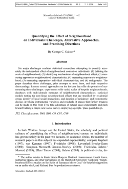


© Copyright 2026