
PDF hosted at the Radboud Repository of the Radboud University
PDF hosted at the Radboud Repository of the Radboud University
Nijmegen
The following full text is an author's version which may differ from the publisher's version.
For additional information about this publication click this link.
http://hdl.handle.net/2066/32995
Please be advised that this information was generated on 2015-02-06 and may be subject to
change.
S o ft-co re m eson -b aryon in tera ctio n s. II. n N and K + N sca tter in g
H. Polinder1,2 and Th.A. Rijken1
1 Institute
fo r Theoretical Physics, Radboud University Nijmegen, Nijmegen, The Netherlands
2Forschungszentrum Jülich, Institut f ü r Kernphysik (Theorie), D-52425 Julich, Germany
arXiv:nud-th/0505083v1 31 May 2005
(Dated: version of: 9th February 2008)
The nN potential includes the t-channel exchanges of the scalar-mesons a and f 0, vector-meson p,
tensor-mesons f 2 and f2 and the Pomeron as well as the s- and u-channel exchanges of the nucleon
N and the resonances A, Roper and S n. These resonances are not generated dynamically. We
consider them as, at least partially, genuine three-quark states and we treat them in the same way
as the nucleon. The latter two resonances were needed to find the proper behavior of the phase shifts
at higher energies in the corresponding partial waves. The soft-core nN-model gives an excellent fit
to the empirical nN S- and P-wave phase shifts up to Tlab = 600 MeV. Also the scattering lengths
have been reproduced well and the soft-pion theorems for low-energy nN scattering are satisfied.
The soft-core model for the K + N interaction is an S U f (3)-extension of the soft-core nN-model.
The K + N potential includes the t-channel exchanges of the scalar-mesons ao, a and fo, vectormesons p, w and p, tensor-mesons a2, f 2 and f2 and the Pomeron as well as u-channel exchanges
of the hyperons A and £. The fit to the empirical K +N S-, P- and D-wave phase shifts up to
Tiab = 600 MeV is reasonable and certainly reflects the present state of the art. Since the various
K + N phase shift analyses are not very consistent, also scattering observables are compared with
the soft-core K+N-model. A good agreement for the total and differential cross sections as well as
the polarizations is found.
PACS numbers: 12.39.Pn, 21.30.-x, 13.75.Gx, 13.75.Jz
I.
IN T R O D U C T IO N
In the previous paper (paper I) [1] the Nijmegen soft
core model for the pseudoscalar-meson baryon interac
tion in general (NSC model) is derived. In this paper
(paper II) we apply the NSC model to the n N and K + N
interactions.
The interaction between a pion and a nucleon has been
investigated experim entally as well as theoretically for
m any years. For the early literature we would like to refer
to Chew and Low [2], who presented one of the best early
models th a t described the low energy P-wave scattering
successfully, Hamilton [3], Bransden and Moorhouse [4]
and Hohler [5].
Although the underlying dynamics of strong hadron in
teractions in general and the n N interaction specifically
are believed to be given by quark-gluon interactions, it
is in principle not possible to use ab initio these degrees
of freedom to describe the low and interm ediate energy
strong interactions. This problem is related to the phase
transition between low energy and high energy strong
interactions and the nonperturbative nature of confine
ment. Instead an effective theory with meson and baryon
degrees of freedom m ust be used to describe strong in
teraction phenomena at low and interm ediate energies,
at these energies the detailed quark-gluon structure of
hadrons is expected to be unim portant.
In particular meson-exchange models have proven to
be very successful in describing the low and interm ediate
energy baryon-baryon interactions for the N N and Y N
channels [6, 7, 8, 9, 10, 11]. Similarly it is expected
th a t this approach can also successfully be applied to the
meson-baryon sector, i.e. n N , K + N , K - N , etc...
Typeset by REVTgX
The last decade the low and interm ediate energy n N
interaction has been studied theoretically, analogous to
the N N interaction, in the framework of meson-exchange
by several authors [12, 13, 14, 15, 16, 17, 18, 19]. The
K + N interaction has been investigated in this framework
only by the Jülich group [20, 21] and in this work. In the
same way as the Nijmegen soft-core Y N model was de
rived in the past as an S U f (3) extension of the Nijmegen
soft-core N N model, we present the NSC K + N -model
as an SU f (3) extension of the NSC nN-m odel.
The above n N meson-exchange models have in com
mon th a t besides the nucleon pole term s also the
A 33(1232) (A) pole term s are included explicitly, i.e. the
A is not considered to be purely dynamically generated as
a quasi-bound n N state, which might be possible if the
n N potential is sufficiently attractive in the P 33 wave.
This possibility was investigated in the past by [22, 23].
From the quark model point of view the A resonance and
other resonances are fundamental three-quark states and
should be treated on the same footing as the nucleons.
We rem ark th a t the exact treatm ent of the propaga
tor of the A and its coupling to n N is different in each
model. The NSC nN -m odel uses the same coupling and
propagator for the A as Schütz et al. [14].
The above n N models differ, however, in the tre a t
ment of the other resonances, P n(1440) (Roper or N*),
Sn(1535), etc... Gross and Surya [13] include the Roper
resonance explicitly bu t the Sn(1535) resonance is gen
erated dynamically in their model, which gives a good
description of the experim ental d ata up to Tlab = 600
MeV. Schutz et al. [14] do not include the Roper res
onance explicitly but generate it dynamically. However
their model describes the n N d ata only up to Tlab = 380
2
MeV, and in this energy region the Roper is not expected
to contribute much. Pascalutsa and Tjon [18] include
the above resonances explicitly in their model in order to
find a proper description of the experimental d ata up to
Tiab = 600 MeV. The resonances th a t are relevant in the
energy region we consider, the A, Roper and S n (1535),
are included explicitly in the NSC nN-model.
Several other approaches to the n N interaction can be
found in the literature, quark models have been used to
describe n N scattering [24]. Also models in the frame
work of chiral perturbation theory exist [25, 26, 27, 28,
29, 30, 31, 32], however, heavier degrees of freedom, such
as vector-mesons, are integrated out in this framework.
We do not integrate out these degrees of freedom, but
include them explicitly in the NSC model.
For the n N interaction accurate experim ental data
exist over a wide range of energy and both energydependent and energy-independent phase shift anal
yses of th a t d ata have been made, e.g.
[33, 34,
35]. Several partial wave analyses for the n N inter
action as well as for other interactions are available at
http://gw dac.phys.gw u.edu/ (SAID).
C ontrary to pions, the kaon (K ) and antikaon ( K in
teraction with the nucleons is completely different. This
is due to the difference in strangeness, which is conserved
in strong interactions. Kaons have strangeness S = 1 ,
meaning th a t they contain an s-quark and a u- or dquark in case of K + and K 0 respectively. Antikaons
have strangeness S = - 1 , meaning th a t they contain an
s-quark and a U- or d-quark in case of K - and K 0 re
spectively. Since the U- or d-quark of the antikaon can
annihilate with a u- or d-quark of the nucleon, the K N
interaction is strong because low-lying resonances can be
produced, giving a large cross section. This situation can
be compared with the A-resonance in n N interactions.
The s-quark of the kaon can not annihilate with one of
the quarks of the nucleon in strong interactions, therefore
three-quark resonances can not be produced, only heavy
exotic five-quark (qqqqs) resonances (referred to as Z * in
the old literature or the pentaquark 0 + in the new liter
ature) can be formed, so the K + N interaction is weak at
energies below the energy of Z *. The cross sections are
not large and the S-wave phase shifts are repulsive.
However, in four recent photo-production experiments
[36, 37, 38, 39] indications are found for the existence of
a narrow exotic S = 1 light resonance in the I = 0 K + N
system with a/s ~ 1540 MeV and T < 25 MeV. The
existence of such an exotic resonance was predicted by
Diakonov et al. [40], they predicted the exotic resonance
to have a mass of about 1530 MeV and a width of less
th an 15 MeV and spin-parity J p = ^ .
The existing K + N scattering data, which we use to fit
the NSC K +N -m odel, does, however, not show this lowlying exotic resonance. On the other hand, this exotic
resonance has not been searched for at low energies in
the scattering experiments. At these energies not much
scattering d ata exists and a narrow resonance could have
escaped detection.
For the early literature on the K + N interaction we
would like to refer to the review article by Dover and
Walker [41]. The K + N interaction has been studied by
the Julich group, they presented a model in the meson
exchange framework, Butgen et al. [20] and Hoffmann et
al. [21], in analogy to the Bonn N N model [9].
In [20] a reasonable description of the empirical phase
shifts is obtained, here not only single particle exchanges,
(a,p,w,A,E,Y*), are included in the K + N model, also
fourth-order processes with N, A, K and K * interme
diate states are included in analogy to the Bonn NN
model, in which a-exchange effectively represents corre
lated two-pion-exchange. Coupling constants involving
strange particles are obtained from the known N N n and
nnp coupling constants assuming S U ( 6 ) sym m etry
However an exception had to be made for the wcoupling, which had to be increased by 60% in order to
find enough short-range repulsion and to obtain a rea
sonable description of the S-wave phase shifts, model A.
B ut this also caused too much repulsion in the higher
partial waves and it was concluded th a t the necessary re
pulsion had to be of much shorter range. In model B the
w coupling was kept at its sym m etry value and a phe
nomenological short-ranged repulsive a 0 with a mass of
1200 MeV was introduced, which led to a more satisfac
tory description of the empirical phase shifts.
In [2 1 ] the model of [20 ] is extended by replacing the aand p-exchange by the correlated two-pion-exchange. A
satisfactory description of the experimental observables
up to Tlab=600 MeV, having the same quality as in [20],
is achieved. Just as in [20] the phenomenological short
ranged a 0 was needed in this model in order to keep the
w coupling at its sym m etry value. Biitgen et al. suggest
th a t this short ranged a 0 might be seen as a real scalarmeson or perhaps as a real quark-gluon effect.
The most recent quark models for the K + N interaction
are from Barnes and Swanson [42], Silvestre-Brac et al.
[43, 44] and Lemaire et al. [45, 46]. The agreement of
these quark models with the experim ental d ata is not
good. The results of [43]- [46] show th a t there is enough
repulsion in the S-waves, but the other waves can not be
described well.
Recently a hybrid model for the K + N interaction was
published by Hadjimichef et al. [47]. They used the
Julich model extended by the inclusion of the isovec
tor scalar-meson a 0(980)exchange, which was taken into
account in the Bonn N N model [9], but not in the
Julich K + N models [20, 21]. The short ranged phe
nomenological a 0-exchange was replaced by quark-gluon
exchange. A nonrelativistic quark model, in which onegluon-exchange and the interchange of the quarks is con
sidered, was used. This quark-gluon exchange is, con
trary to the a 0-exchange, isospin dependent. A satisfac
tory description of the empirical phase shifts, having the
same quality as [21], was obtained. However Hadjimichef
et al. conjecture th a t the short ranged quark-gluon dy
namics they include could perhaps be replaced by the
exchange of heavier vector-mesons.
3
Another approach for the K + N interaction is given by
Lutz and Kolomeitsev [32]. Meson-baryon interactions in
general and K + N interactions specifically are studied by
means of chiral Lagrangians in this work. A reasonable
description of the K + N differential cross sections and
phases was achieved, bu t only up to Tlab = 360 MeV.
The m ajor differences between the existing n N and
K + N models and the NSC model presented in this work
are briefly discussed below. Form factors of the Gaus
sian type are used in the soft-core approach in this work,
while monopole type form factors and other form factors
are used for the nN -m odel by Pascalutsa and Tjon [18]
and the K + N-model by Hoffmann et al. [21]. The Roper
resonance in the n N system is, at least partially, consid
ered as a three-quark state and treated in the same way
as the nucleon and is included explicitly in the poten
tial. However, we renormalize the Roper contribution at
its pole, while Pascalutsa and Tjon [18] renormalize it at
the nucleon pole.
An other difference is our treatm ent of the scalarmesons a etc., we consider them as belonging to an
S U f (3) nonet, while in all other models they are con
sidered to represent correlated two-pion-exchange effec
tively. Also we include Pomeron-exchange, where the
physical nature of the Pomeron can be seen in the light
of QCD as (partly) a two-gluon-exchange effect [48, 49],
in order to comply with the soft-pion theorems for lowenergy n N scattering [50, 51, 52]. Furtherm ore, the ex
change of tensor-mesons is included in the NSC model
m ainly to find a good description of the K + N scatter
ing data. We use only one-particle exchanges to find this
description while Hoffmann et al. [21] need to consider
two-particle exchanges in their K + N-model.
The contents of this paper are as follows. In Sec. II
the SU f (3) relations between the coupling constants used
in the n N and K + N interactions are shown. The n N
total cross section shows several resonances in the con
sidered energy range. The renorm alization procedure we
use to include the s-channel Feynman diagrams for the
resonances in the n N potential is described in Sec. III.
In Sec. IV the NSC nN -m odel is discussed and the re
sults of the fit to the empirical phase shifts of the lower
partial waves are presented. The NSC nN -m odel is, via
SUf (3)-symmetry, extended to the NSC K +N -m odel in
Sec. V. The results of the fit to the empirical phase
shifts are given, since the different phase shift analyses
are not always consistent, also the model calculation of
some scattering observables is given. The NSC K + N model is used to give a theoretical estim ate for the upper
limit of the decay width of the recently discovered exotic
resonance in the isospin zero K + N system.
Finally the sum m ary gives an overview of the research
in this work and its main results. Also, some sugges
tions for improvement and extension of the present NSC
model are given. In Appendix A details are given on
the calculation of the isospin factors for n N and K + N
interactions.
II.
M E SO N -B A R Y O N C H A N N ELS AN D SUf (3)
We consider in this work the n N and K + N interac
tions, they make up only a subset of all meson-baryon in
teractions. Because the NSC K + N-m odel is derived from
the NSC nN-m odel, using SU f (3) symmetry, we define
an SU f (3) invariant interaction Hamiltonian describing
the baryon-baryon-meson and meson-meson-meson ver
tices. The Lorentz structure of the baryon-baryon-meson
interaction is discussed in paper I , here we deal with its
SUf (3) structure. In order to describe the interaction
Hamiltonian we define the octet irreducible representa
tion (irrep) of S U f (3) for the J p =
baryons and the
octet and singlet irreducible representations of SU f (3)
for the mesons. Using the phase convention of [53], the
Jp =
baryon octet irrep can be w ritten as traceless
3 3 m atrix
£+
£-
B
S°
,
p
n
A
770
\
(2.1)
2A
V6
similarly the pseudoscalar-meson octet irrep can be writ
ten as
n+
K+
_ tlL , m_
o
V i + Ve
1X
0
_ 2j»
V6
P8 =
\
(2.2)
while the pseudoscalar-meson singlet irrep is the 3 x 3
diagonal m atrix P i with the elements
on the di
agonal. The pseudoscalar-meson nonet, having a nonzero
trace, is given by
P
(2.3)
P8 + Pi •
The physical mesons n and r/' are superpositions of the
octet and singlet mesons n8 and r 1, usually w ritten as
n' = sin o n8 + cos o ni
(2.4)
r = cos o r 8 —sin o ni
Similar expressions hold for the physical coupling
constant of the n and n7. The octets and singlets for the
scalar- and vector-mesons are defined in the same way
and the expressions for the physical (w,y>) and ( a ,f 0)
are analogous to (n 7,n). From these octets and nonets,
SU f (3)-invariant
baryon-baryon-meson
interaction
Hamiltonians can be constructed, using the invariants
Tr (B P S ), Tr ( B B V ) and Tr ( B B ) Tr ( P ). We take the
antisym m etric ( F ) and symmetric (D) octet couplings
and the singlet (S) coupling
\ B B P \ p = Tr ( B P B ) - Tr ( B B P )
= Tr (B P 8B) - Tr ( B B P 8) ,
[B B V ]
2
d
= Tr { B P B ) + Tr ( B B P ) - | T r ( B B ) Tr (P)
4
= Tr (B P s B) + Tr (BBPs) ,
[8 8 P ] S = Tr (¡38) Tr ( P ) = Tr (8 8 ) T r(P i) .
(2.5)
The SUf (3)-invariant baryon-baryon-meson interaction
Hamiltonian is a linear combination of these quantities
and defined according to [53]
m v+H = f s V 2 ( a [ B B V ] f + (1 - a) [B B P ]
) +
The baryon-baryon-meson vertices are thus characterized
by only four param eters if SU f (3)-sym metry is assumed,
the octet coupling constant f s , the singlet coupling con
stant f i, the F / ( F + D )-ratio a and the mixing angle,
which gives the relation between the physical and octet
and singlet isoscalar mesons. The SUf (3) invariant local
interaction densities we use for the triple-meson (MMM)
vertices are given below.
(i) J p c = 1
(2.6)
Here, a is the F / ( F + D )-ratio. The most general inter
action Hamiltonian th a t is invariant under isospin trans
formations is given by
m ^+H i
[¡N Nn i (N N ) + f AAm (AA) + Zssni (S • S
m n+ Hs
+ / HHm (S S )] ni ,
f N Nn ( N T N ) • n -
H
gPPV fabc V a P
ppv
gppv
p M• ( n x d
^¿K*t
tK
(S >( S ) • 7T
i—
+ f NNns (N N ) ns + f AAns (AA) ns
(2.7)
+ f ESns (S • S ) ns + f HHns (S S ) ns •
for the singlet and octet coupling respectively, and
f N N n = f 8 and f NNn1 = f AAni = f EEni = f HHni = f 1We have introduced the isospin doublets
= (K :),K c= ( J !
(2.8)
the phases have been chosen according to [53], such th at
the inner product of the isovectors S and n is
(2.9)
The interaction Hamiltonians in Eq. (2.7) are invariant
under SUf (3) transform ations if the coupling constants
are expressed in term s of the octet coupling f s = f and
a as, [53],
rj + H .c )) +
^-*1 ^
9
A
,
(2-12)
f NNn8 = 4V3j ( 4 a - l ) /
2 a)f
“ V3(1
f EEn8
v/3^1 a W
f AAr/8
“ aW
f HAK = ^ ( 4 a - l ) f
f HEK = - f
(2.10)
and the singlet coupling f i as
(ii) J p c = 0++ Scalar-mesons:
H
pps
=
g p p s dabc S a P b P c
g p p s T r Ps (Ps • S s + S s • Ps)
2 a/ 2
gpps
fN N n = f
2
a0 • f
tti] + ^ - K ^ t K
J+
( k I t R ■Tr + H . c ) - - ( K l K r , + H .c.
8
[I]
a)f)
—
1
f NNrn = f AAni = f EEni :
K) +
for the derivative d acting on the pseudoscalar«-►ft
mesons, P b d P c = P b (dMP c) —(dMP b) •P c. The
coupling of the vector-mesons to the pseudoscalarmesons is SU f (3) antisymmetric, the symmetric
coupling can be excluded by invoking a general
ized Bose sym m etry for the pseudoscalar-mesons,
interchanging the two pseudoscalar-mesons leaves
H PPV invariant. The coupling constant for the
decay of a p-meson into two pions is defined as
gnnp = 2 gPPV, which can be estim ated using the
decay w idth of the p-meson, see Eq. (4.9).
+ f SHK [55 • (K ] t S) + (S T"Kc) • S]
= —( 1 —2 a) ƒ
=
= 2a f
= - ^ a + 2 « )/
= ( 1 —2 a ) f
n + iK tT d
where H.c. stands for the Herm itian conjugate of
the preceding term, and we use the usual notation
+ fsN K [S • ( K t TNT) + (N t A ) • 5)]
f-Hn
f AEn
fEEn
fANK
fENK
j.
\/3 *p8,pi A
+f-A K [(S Kc) A + A ( K ts ) ]
S • n = S + n - + S V + S - n+
PC
• ¿T n + H .c.) +
(iK * jK T
+ f a n k [(NTK) A + A(KtNT)]
r ) , K
d
- i V 2 g p p v T r V 8 (dMP 8 ■V8M- V8M dMP 8)
+ f AEn (A S + S A ) • n + f HHn (STS
N
Vector-mesons:
=.ni
fi .
(2.11)
+ -fa
( t v -TV -
K ]K - ip-/)
(2.13)
For the scalar-mesons we have a symmetric cou
pling. The dimensionless coupling constant for the
decay of the a-meson into two pions is defined as
gnna = gPPS/ m n+, which can be estim ated using
the decay w idth of the a-meson, see Eq. (4.9).
5
(iii) J p c = 2++ Tensor-mesons:
+
H
2gp PT
—
mn+
ppt
a 2V • (
+ ^-d ^K W d vK
V,
Vs
^3
+ ^ Y ( K ^ T d ^ K ■¿>„7T + F .c .) 2
Figure 1: The pole potential Vs contains s-channel diagrams,
the non-pole potential Vu contains t- and u-channel diagrams.
^ ( K ^ d „ K d vV + H . c .)
+ x / 2 tI/ ( ^ t t ' ^
7r -
d^K^dvK - d ^ d ^ )
V ( p '; p) — Vs (p /, p) + V„(p', p) 1, see Figure 1, where
(2.14)
The coupling constant for the decay of the f 2-meson
into two pions is given by gn n /2 — gPPT, which is
estim ated in Eq. (4.9).
Some numerical values for the previous coupling con
stants are given by Nagels et al. [54]. The isospin factors
resulting from the previous interactions are discussed in
Appendix A and listed in Tables I and VII for n N and
K + N interactions respectively. We rem ark th a t in the
NSC model the SUf (3)-symmetry is broken dynamically,
since we use the physical masses for the baryons and
mesons. The SUf (3)-symmetry for the coupling con
stants is not necessarily exact, in fact, we allow for a
breaking in the NSC K +N -m odel, Sec. V .
III.
R E N O R M A L IZ A T IO N
The Lagrangians used are effective Lagrangians, ex
pressed in term s of the physical coupling constants and
masses. Then, in principle, counter-term s should be
added to the Lagrangian and fixed by renorm alization
conditions. This is particularly to the point in channels
where bound-states and resonances occur. For example,
the famous A resonance at M a — 1232 MeV in the n N
system. The A pole diagram gets “dressed” when it is
iterated with other graphs upon insertion in an integral
equation. Also, it appears th a t by using only u-channel
and t-channel forces it is impossible to describe the ex
perim ental n N phases above resonance in the P 33-wave.
From the viewpoint of the quark-model this is natural,
because here the A resonance is, at least partly, a gen
uine three-quark state, and should not be described as a
pure n N resonance, bu t should be treated at the same
footing as the nucleons. We take the same attitu d e to the
other meson-baryon resonances as the Roper, Sn(1535),
etc. The resonance diagrams split nicely into a pole part,
having a ( / — Mn+*e)_ 1 -factor, and a non-pole p art hav
ing a ( / + M q — ¿e)_ 1 -factor. Here, M q is the so-called
“bare” mass. The pole-position will move to / = M r ,
where M r is the physical mass of the resonance. This
determines the bare mass M 0.
To implement these ideas, we follow Haymaker [55].
We write the to tal potential V as a sum of a poten
tial containing poles and a potential not containing poles
a
a
Vs(p/,p ) — ^ ( p O
a
(3.1)
is the pole part of the s-channel baryon exchanges. In
Eq. (3.1) the right hand side is w ritten in term s of
the so-called “bare” couplings and masses. We have
A i ( P ) = ( / — M q + ie)_1, where in the CM system
P = ( / , 0). The other part and the i-channel and uchannel exchanges are contained in Vu(p /, p). In the fol
lowing, we trea t explicitly the cases when there is only
one s-channel bound state or resonance present. It is easy
to generalize this to the case with more s-channel poles.
Following [55] we define two T -m atrices T j, j — 1, 2 by
a
a
s
s
Tj — V,- + V,- G T , T — T 1 + T 2
(3.2)
where Vi — Vs and V2 — VU. The am plitude T, is the sum
of all graphs in the iteration of T in which the potential
Vj “acts last” . Defining Tu as the T -m atrix for the VU
interaction alone, i.e.
Tu — VU + VU G Tu ,
(3.3)
it is shown in [55] th at
Ti — T„ + T„ G T 2 , T 2 — Ts + Ts G T„ ,
(3.4)
Ts — Vs + Vs H i Ts , H i — G + G T „ G .
(3.5)
with
Taking together these results one obtains for the total
T -m atrix the expression
T — T„ + Ts + T„ G Ts + Ts G T„ + T„ G Ts G T„ . (3.6)
Since Vs is a separable potential, the solution for Ts in
the case of one pole can be w ritten as
s
s
A i(P ) F j(p)
i
T s(p/, p)
r (p ) r(p) = F(p/) A*(p) r(p) ;
A (P )- 1 - £ ( P )
(3.7)
s
1 Notice th a t in [55] th e V - and T -m atrices differ a (-)-sign with
those used here.
6
where we introduced the shorthand A — A i , and defined
the self-energy E and the dressed propagator A* by
dq' / dq'' r ( q ') H i(q ', q"; P ) r ( q '') ,
E (P ) =
A (P )
A * (P ) =
1 - A (P ) E (P )
= A ( P ) + A ( P ) E ( P ) A * (P )
T
V
V
Vu
A
T
T
-1 u
A*
T
■
iu
Vu
r.
r
(3.8)
where dq/ — d 3 q//( 2 n ) 3 etc.. Inserting Eqs. (3.7) and
(3.8) in Eq. (3.6), and exploiting time-reversal and parity
invariance, which gives Tu (p /, p) — T„(p, p /), one finds
the expressions for the total amplitude, dressed vertex
and self-energy
+
Tu
g
r
g
r
T (p /, p) — T „(p/, p) + r * ( p /) A * (P ) r* (p ) , (3.9)
[------ -—
A*
[------- — 1-1
r* (p ) — r ( p ) + y dq r(q )G (q ,P )T „ (q , p) (3.10)
E ( P ) — ƒ dq r ( q ) G ( q ,P ) r* (q ) ,
(3.11)
where the dressed propagator A * (P ) is given by
A * (P ) - 1 — A (P ) - 1 - E (P ) .
(3.12)
The equations above show th a t the complete T-m atrix
can be com puted in a straightforw ard manner, using the
full-off-shell T -m atrix T u ( p ' , p ) , defined in Eq. (3.3).
The renormalized pole position yjs = M r is determ ined
by the condition
0 = A *(^7s = M r )
=
A (y /s
=
M r)-1 -
E ( a / s
=
Mr)
.
(3.13)
P a rtia l wave analysis
The partial wave expansion for the vertex function r
reads
r(P) = Æ
^ r ^ ^ p ) ,
L,M
(3.14)
and similar for r* . The partial wave expansions for the
am plitude T reads
T (q, p ) = 4^ ^ TL(q ,p )
L,M
In the following subsections it is understood th a t we deal
with the partial wave quantities. We suppress the angu
lar mom enta labels for notational convenience.
- 1
A diagram m atic representation of the previous derived
equations for the meson-baryon amplitude, potential,
dressed vertex and dressed propagator is given in Fig
ure 2 .
A.
Figure 2: The integral equation for the amplitude in case of a
non-pole and pole potential, a. integral equation for the total
amplitude , b. the potential in terms of the non-pole and pole
potential, c. the amplitude in terms of the non-pole and pole
amplitude Eq. (3.9), d. integral equation for the non-pole
amplitude Eq. (3.3), e. equation for the dressed vertex Eq.
(3.10), f. equation for the dressed propagator Eq. (3.12).
y M(q )*
YM(p) •
(3.15)
Then, the partial wave projection of the integrals in Eqs.
(3.10) and (3.11) become
B.
M ultiplicative renorm alization p aram eters
To start, in Eq. (3.9) the second part on the right
hand side we consider to be given in term s of the bare
resonance mass M 0 and the bare resonance coupling g0.
We consider only the wave function and vertex renor
m alization for the resonance, and use the m ultiplica
tive renorm alization method. Then, since the total Lagrangian is unchanged and hermitian, unitarity is pre
served. The Z-transform ation for the resonance field
reads
and for the resonance coupling
g0 — Zg gr , where the subscripts r and 0 refer to respec
tively the ’’renormalized” , and ”bare” field. Applied to
the A N n interaction this gives
Ci ~
= Z g \ [ Z ~2 g r^ r^ ip d ^ c t) ,
where gr — fA Nn/ m n+ is the renormalized, i.e. the phys
ical, and go the unrenormalized, i.e. the bare coupling.
Introducing the renorm alization constant Z \ = Z g y [ Z o,
we have
Li -
r L(p) = y l ( p ) + t ^ J q 2 < k r L (q) G ( q , P ) T u,L (q ,p ) ,
EL(P) = ¿
/ <Z2 d? r L(g) G(q,P) r£(q) .
(3.16)
(3.17)
Z 1 gr <I>r,M^ d M^
— g r f r ,M^ d M^ + (Z 1 - 1)gr 't r ,M^ d M^ . (3.18)
From the form of Eq. (3.10) it is useful at this stage
to distinguish functions with the bare and physical cou
7
plings g0 and gr . Therefore, we introduce the vertex func
tions
r U,r (p ) — r u,r (p ) + ƒ dq r u,r (q) G (q) Tu (q,p ) ( (3.19)
term s of the renormalized quantities the am plitude Tr
of Eq. (3.22) reads
1
Tres(p /,p ) = r *en(P/ )
a/
w ith the definitions
ru,r(p) — g 0,r r ( p ) , ru,r(p) — g0,r r * ( p ) ,
(3.20)
implying the relations
=
^
s
i 2) ( v ^ )
M r — SreL ( af s )
, r * e„ ( p )
ili
TreS(p',p) = r U(p )
a/s —M q — Yju ( a/s )
r u ( p ) . (3.22)
Next, we develop the denom inator around the renorm al
ized, i.e. the physical, resonance mass M r and rearrange
terms. We get
Tres(p /,p ) = r U( p )
a/
( a/
s
—
—
ru(p)
1
as«
9 a/
s
( a/
rU(p)
’ ’
M r) -
-
s
1
(3.23)
Here, we have introduced the renorm alization constant
Z 2 defined by
1—
dSu
<9 a/
s
s/ s= M r j
-1
1 + Z‘ §O /T
a
(3.24)
s
The derivatives in Eq. (3.23) w.r.t. / are evaluated at
the point / = M r, as is indicated in Eq. (3.24).
Now we require th a t the residue at the resonance pole
is given in term s of the physical coupling, i.e. gr . In
a
a
—
M r)
s
(3.27)
\fs=MR
We notice th a t the im aginary p art of the self-energy is
not changed by the wave function renormalization. It is
straightforw ard to include 9 S (a /s)ìii the resonance mass
M r as well as in E ren(y/s).
The com putation of the am plitude Tres(p/,p), Eq.
(3.25), using renormalized quantities only runs as fol
lows. From Eqs. (3.21) and (3.26) and the definition
Z \ = Z g ^ fZ n the renormalized vertex is given by
(3.28)
N otice th a t r* ( p r ) — |r*(pR)| exp(*p>*(pr)), a nd th at
this phase can be ignored w h e n defining the effective decay
L agrangian i n Eq. ( 3 .1 8 ) . The renorm alization condition
for the vertex is th a t at the pole position (a/s = M r ) the
renormalized vertex is given in term s of the physical cou
pling constant
| grT* (P = Pfl ) | = gr ^ y / E R + M ,
(3.29)
which determines Z 1 and, by Eq. (3.24), Z 2 and Zg,
now the renormalized self-energy and the renormalized
dressed vertex are known from Eq. (3.26). In passing
we note th a t the coupling gr — fA Nn /m n , and the other
factors in the second expression of Eq. (3.29) are specific
for a P 33-wave resonance.
A s is clear fr o m this sectio n one can either express all
qua ntities i n te rm s o f the bare p a ra m eters (M 0 ,g 0) or in
te r m s o f the reno rm alized p a ra m eters (M r, gr ).
1
Z2 =
s
+ ...
=Mr
S ren (M r )
. ¿»E.
<9 a/
lr ren(P = Pfi)l =
= r ; ( p /)Z 2 r ; ( p )
( a/
( W
r*en (P) = Z i C (P)
M r) —
( a/ s - M r )
(3 .2 6 )
1
d Su
(a/s —M r )
rU(p')
^ren(V ^)
/ r-
M o — T,u ( M r ) —
-
s
.
\ 2 d ~ Y j r en
5 (v /I“ m “ )
1
=
s
^ ! r
Resonance renormalization
Working out this renorm alization scheme for the
baryon resonances, we start, in Eq. (3.9) with the second
p art on the right hand side as given in term s of the bare
resonance mass M 0 and bare resonance coupling g0. We
write this p art of the am plitude as
r*en(p) .
The renormalized self-energy in the last expression in Eq.
(3.23) and its first derivative are defined to be zero at the
resonance position / = M r and is given by
a
1.
—
(3.25)
Here we have defined the renormalized self-energy and
the renormalized dressed vertex
^ r e l ( % /s )
r u (p ) — Zg r r (p ) ( r U(P) — Zg r *(p ) (
E „ ( P ) — Zg2 Er ( P ) .
(3.21)
s
s
For the second p art of this statem ent we now express
the bare quantities in term s of the renormalized ones.
From Eqs. (3.24) and (3.29) we know Zg, thus
g2
g0
= Z2 g 2
=
gr
(3.30)
s
In the following, we denote the real p art of the resonance
mass by M r . Also, we want to renormalize at a point
8
which is experim entally accessible. Therefore, we choose
for the renorm alization point the real part of the reso
nance position, a/s = M r . So actually we consider the
real part of the self-energy, KS, in the previous deriva
tions and from Eq. (3.23) we have
M r = Mo +
^ S (M r ) ,
(3.31)
giving the bare mass in term s of the renormalized quan
tities
Mo = M r - Z„V2 K Ê (M r)
(3.32)
T h is concludes the d e m o n s tr a tio n th a t one m a y start
w ith the p hysical p a ra m eters a nd com p u te the bare p a
ra m eters (go, Mo). O f course, in exploiting Mo i n order
to force the pole p o sitio n at the chosen a/s = M r to be
reasonable one m u s t have Mo > 0 .
Substituting this again in Eq. (3.5) one finds
A - (p )£ij -
r i (p)
r i( p " ) x
H i( p ", p '; P ) r j ( p ') A j(P )A j (p) (3.36)
which can be solved, and leads to the separable TS-matrix
Ts(p ', p ) = 5 3 r i (p 7)
a -1 (p ) -
/ r(p ") x
l
r j (p )
l
= E
r i (p ' )
A - i (P ) - S (P )
r j (p)
(3.37)
2.
Nucleon pole renormalization
The renorm alization of the nucleon pole is completely
analogous to the resonance renormalization, except for
the renorm alization point, which is now the nucleon mass
and thus below the n N threshold. Here the G reen’s
function has no pole and is real. This implies th at
K S (M n ) = S (M n ), in contrast to the resonance case.
All quantities in the expression for the self-energy, Eq.
(3.11), are real at the nucleon pole.
The renorm alization condition for the vertex, analo
gous to Eq. (3.29), is th a t at the nucleon pole position
( a / s = M n ) the renormalized vertex is given in term s of
the physical coupling constant
lr *en(P =
)|
Z i |grr*(p = ipw)
fr
a/
3
i pN
( a/ s + M ) (3.33)
in case of pv-coupling. This determines the renorm al
ization constant Z i. In passing we note th a t the factor
in the second expression of Eq. (3.33) is specific for a
P 11-wave nucleon pole. Since the nucleon pole position
lies below the n N threshold, r* (ip N) and in Eq. (3.10)
r ( ip N ) and Tu (q,
) are imaginary.
C.
G en eralization to th e m ulti-pole case
In case of multiple pole contributions we have the gen
eralized expression for the pole potential Eq. (3.1)
W
, p) = Ç W
i
) A j(P ) Ei(p) .
(3.34)
From Eq. (3.5) one finds, using Eq. (3.34) th a t the pole
am plitude Ts can be w ritten as
Ts(p ' , p) = E r i ( p ' ) A i(P ) A i(p) .
(3.35)
which obviously is a generalization of Eq. (3.7). In Eq.
(3.37) the quantities A - 1 ( P ), r ( p ) , and H 1 (p", p '; P )
stand respectively for a diagonal m atrix, a vector, and a
constant in resonance-space. Above, we have introduced
the generalized self-energy in resonance-space as
S ij ( P ) = f f r 4(p") H 1 (p", p '; P ) r j ( P ) .
D.
(3.38)
B aryon m ixing
In this paragraph we consider the case of two differ
ent nucleon states, called N 1 and N 2. A part from their
masses they have identical quantum numbers. In par
ticular, this applies to the (I =
= ^ + )-states
N and the Roper resonance, i.e. the P 11 -wave. Obvi
ously, the resonance-space is two-dimensional. Starting
with the bare states N 1 and N 2, these states will com
m unicate with each other through the transition to the
nN -states, and will themselves not be eigenstates of the
strong Hamiltonian. The eigenstates of the strong Hamil
tonian are identified with the physical states N and the
Roper, which are m ixtures of N 1 and N 2. To perform the
renorm alization similarly to the case with only one reso
nance, we have in order to define the physical couplings
at the physical states to diagonalize the propagator. This
can be achieved using a complex orthogonal 2 x 2 -m atrix
O , G O = O O = 1. We can write, similar to Pascalutsa
and Tjon [18],
O
cos x sin x
sin x cos x
where x is the complex
since N 1 and N 2 have the
from their couplings and
isomorphic. This implies
(3.39)
(N 1, N 2)-mixing angle. Now,
same quantum numbers, apart
masses, their nN -vertices are
th a t the self-energy m atrix in
9
Eq. (3.38) can be w ritten as
2
S 1 1 (P ) S 12 (P)
S 21 ( P ) S 22 ( P )
u
gWiWn SW2WT
SNiNn
SNiNn g» 2«n
gN2Nn
£ ( P ) , (3.40)
u
while for the vertices we have
r Ni
r N2
formulate the procedure in term s of the bare or unrenor
malized param eters and not directly in term s of the phys
ical param eters. This way we can utilize Eqs. (3.40) and
(3.41). As we will see, we get four equations from the
renorm alization conditions on the masses and couplings,
with the set of four unknowns {Mo,1, M o,2, go,1, go,2}.
For both a-solutions we have, using M o = (M o, 1 +
M o 2 )/2, th a t the resonance am plitude is
1
SNiNn
9 N2N1
(3.41)
Tres(a) = r « ( a ,p ')
The propagator in Eq. (3.37) is diagonalized by the angle
r «( a ,p )
u
r .
u
SNiNn
S^N n
x (P ) = - arctan 2
2
SW2WT
SNiNn
SNiNn SN2Nn S (P ) u
a / s — M q — S ( a , M r ( ol ) ) —
= r «( a ,p )
(3.42)
( a/ s
- M R (a)) -
r « ( a , P)
9 a/
A * ( P ) - X(± ) = v ^ - i ( M o
S (± ,P ) =
,1
Z (a )
1
d'E(a)
We write S = S u in the following for notational conve
nience. The corresponding eigenvalues are
r « ( a ,p )
r « ( a ,P)
'''_
d yfs
(a/s - M R ( a ))
=
1
d’E(a)
(a/s - M R ( a ))
1
Mjy2 - M Wl
r « ( a ,P)
aJ~s — M q — S ( a , a / s )
' '
s
( a/ s
r « ( a ,P)
- M R (a ) —
+ Mo, 2 ) - £ ( ± , P ) ,
<92£ (a )
—(a/s —M R{ a ) Y Z (a)
2
(¿ W
[ ( S u ( P ) + S 22 ( P )) ± [(M o ,2 - Mo,1
+ S 22 ( P ) - S 1 1 ( P ) ) 2
+ 4S 12(P )2] 1/2]
/2
.
(3.43)
,(3.46)
here we introduced the renorm alization constants Z (a )
defined by
1
Here, we denoted the unrenorm alized masses by Mo,1 =
MNi for the nucleon, and by Mo ,2 = MN 2 for the Roper
resonance. Likewise, the unrenormalized couplings are
denoted as go,1 = SNiNn,« and go,2 = SN2Nn,u. Then,
for example S j ( P ) = g o ^S o jS (P ). The resonance am
plitude Tres is a generalization of the second term in Eq.
(3.9) and can be rew ritten as follows
dS
Z (a )
\/s — —(A/o,i + M q^ ) — S (a , P ). (3.45)
Unlike in [56] we renormalize the eigenstate a = (—)
at the nucleon pole, and the eigenstate a = (+ ) at the
Roper resonance position. T hat is the reason why we
2 Notice th a t we distinguish th e nucleon in th e n N -sta te from
N i ,2 -states.
s
= M
r
( o C) y
(af i s - M R {a))
2 ¿>2S ren(a)
(¿ W
a/
s
)
+ ..
— S re n (a , M r (a ) ) —
(a/s - M R ( a ))
OYjren {&)
(3.48)
9 a/ s
where the derivatives are evaluated at the point a/ s =
M R(a). The resonance am plitude Tres(a) in Eq. (3.46)
in term s of the renormalized quantities reads
T res{o.)
da { P ) =
1
-
S r e n (oi,
= E (r* (p ' )O)i (<5a *(p ) o ) .. ( O r » ) ,
i
where the diagonalized propagator is
/
Also we can define S ren(a, a/ s ) = Z ( a ) Y , ( a , a/ s ) similar
to Eq. (3.26). Analogous to Eq. (3.27) we introduce the
renormalized self-energy by
Tres(p ',p ) = E r**(P') A*j (P )r* (p )
ij
E (r* (P )O )a d - 1 ( P ) (O r* (p ))^ ,(3.44)
a=±
(3.47)
1 <9 a/ s
S ri(a ,
=
=
(a )
=
T*e n ( a , p ' )
a /s -
M fl(a )
-
S ^ }n ( a , a / s )
x r * e„ (a ,p ) ,
(3.49)
where the renormalized vertex is
r : e„ (a ,p ) = v /^ ) r > , p ) .
(3.50)
In the previous we have suppressed the m om entum de
pendence of Tres(a) for notational convenience. The
renorm alization is now performed by application of the
following renorm alization conditions:
10
(i) M ass-renormalization: The physical masses M R(a)
are given implicitly by
M R(a) = M o + S (a M R(a)) .
(3.51)
(ii) Coupling-renormalization: The physical coupling
constants gr (a) are given by
lim
V s—>Mr (cx)
Figure 3: Contributions to the nN potential from the s-, uand t-channel Feynman diagrams. The external dashed and
solid lines are always the n and N respectively.
( y f s - M R ( a ) ) T res(a)
= |r* e„ (a ,p R )|2
= Z (a ) |ru ( a ,p R )|2 .
Eqs.
(3.51) and (3.52)
These can be solved for
{Mo,1 , Mo,2 , So,1 , go,2} using
and coupling constants. We
(3.52)
constitute four equations.
the four bare param eters
as input the physical masses
get
go,1 = go,1 [gr (+ ),g r ( —); M R(+ ),M R( —)] ,
So,2 = So,2 [Sr(+ ) , Sr( —) ; M R( + ),M R( —)] ,
M o,1 = M o,1
Sr( —); M R(+ ),M R( —)] ,
M o,2 = M o,2
Sr( —); M R(+ ),M R( —)] . (3.53)
shift analysis of A rndt et al.[33] (SM95) . We find a good
agreement between the calculated and empirical phase
shifts, up to Tlab = 600 MeV for the lower partial waves.
The results of the fit to the A rndt phase shifts are shown
in Figure 6 . The calculated phase shifts are also com
pared with the Karlsruhe-Helsinki phase shift analysis
[34] (KH80) in Figure 7. The param eters of the NSC
nN -m odel are given in Tables III and IV .
Some results of the renorm alization procedure for the
s-channel diagrams, discussed in Sec. III, are given. The
bare coupling constants and masses are listed in Table
IV, and the energy dependence of the renormalized self
energy of the nucleon and A are shown in Figure 5.
From these we obtain the renorm alization constants:
A.
Zg( —) = S,o,1 / S,r ( —) , Zg( + ) = S'o^SV(+ ) .
Notice th a t after the diagonalization of the propagator
we have two uncoupled systems a = ± . Therefore, it is
n atural to define, in analogy with the single resonance
case, the Z 1 (a)-factors by
r *en(a >P) = V z 2 (a) r*(a,p)
= Z 1 (a) Z- 1(a) r u ( a ,p )
= Z 1 (a) r* ( a ,p ) ,
(3.55)
where Z 2 (a) = Z (a ).
R otating back to the basis
(N 1 ,N 2) we find the Z-transform ation on the original
basis before the diagonalization of the propagator. This
Z-transform ation on the unmixed fields is a 2 x 2-matrix.
Note, th a t in Eqs. (3.54) and (3.55) we have defined
several Z-factors suggestively. In order to find out how
these constants are related to the Z-m atrices alluded to
above, we would have to work out this Z-transform ation
in detail. This we do not attem pt, since it is not really
necessary here.
From the input of the four physical param eters
{M R(a ),S r (a)} one computes the bare param eters. Us
ing the latter one computes Eren(a, a / s ) and r*en(a,p).
This defines the resonance p art of the am plitudes unam
biguously.
IV.
T he NSC nN -m odel
(3.54)
T H E nN IN T E R A C T IO N
In this section we show the results of the fit of the NSC
nN -m odel to the most recent energy-dependent phase
The potential for the nN -interactions consists of the
one-meson-exchange and one-baryon-exchange Feynman
diagrams, derived from effective meson-baryon interac
tion Hamiltonians, see paper I and Sec. II. The diagrams
contributing to the n N potential are given in Figure 3.
The partial wave potentials together with the n N G reen’s
function constitute the kernel of the integral equation for
the partial wave T -m atrix which is solved numerically to
find the observable quantities or the phase shifts. We
solve the partial wave T -m atrix by m atrix inversion and
we use the m ethod introduced by Haftel and Tabakin
[57] to deal numerically with singularities in the physical
region in the G reen’s function.
The interaction Hamiltonians from which the Feynman
diagram s are derived, are explicitly given below for the
n N system. We use the pseudovector coupling for the
N N n vertex
H
un
* =
{N js^
t
N) ■
,
(4.1)
the same structure is used for the Roper, and for the
£11(1535) we use a similar coupling where the 75 is om it
ted. The N N n coupling constant is quite well deter
mined and is fixed in the fitting procedure. For the N A n
vertex we use the conventional coupling
Una* =
— — (A m2 W ) . ¿ ^ tt + H .c. ,
mn+
(4.2)
where T is the transition operator between isospin-^
isospin-1 states [58]. The only vector-meson exchanged
11
in n N scattering is the p. The N N p and nnp couplings
we use are
+
n nnp
4M
gnnp
(4.3)
we rem ark th a t the vector-meson dominance model pre
dicts the ratio of the tensor and vector coupling to be
= f NNp/g NNp = 3.7, but in n N models it appears
to be considerably lower [12, 16, 17, 18]. We also find
a lower value for k p, see Table III. The scalar-meson
couplings have the simple structure
(4.4)
H nnct = gwNff N N a ,
Hn
2
-m ^+aîr • 7T
(4.5)
In contrast with other n N models, we consider the
scalar-mesons as genuine SU f (3) octet particles. There
fore not only the a is exchanged bu t also the fo(975)
having the same structure for the coupling, both giv
ing an attractive contribution. The contribution of aexchange is, however, much larger than the contribution
of fo-exchange. A repulsive contribution is obtained from
Pomeron-exchange, also having the same structure for
the coupling. The contributions of the Pomeron and the
scalar-mesons cancel each other almost completely, as can
be seen in the figures for the partial wave potentials, Fig
ure 4 . This cancellation is im portant in order to comply
w ith the soft-pion theorems for low-energy n N scatter
ing [50, 51, 52]. The a and the p are treated as broad
mesons, for details about the treatm ent we refer to [59].
The a is not considered as an SUf (3) particle in other
n N models, but e.g. as an effective representation of
correlated two-pion-exchange [14, 15, 18], in th a t case its
contribution may be repulsive in some partial waves.
We consider the exchange of the two isoscalar tensor
mesons f 2 and f 2 , the structure of the couplings we use
¿Fil N N f 2
NM
4
F o N N f2
~
n
N
ym dv
+Yv
vN
N
f2
^
f r (9M7T • d v 7T) ,
m n+
(4.6)
and the coupling of f2 is similar to the f 2 coupling. Simi
lar as for the scalar-mesons fo and a, the f 2 contribution
is very small compared to the f 2 contribution.
The isospin structure results in the isospin factors
listed in Table I, see also Appendix A . The spin-space
am plitudes in paper I need to be multiplied by these
isospin factors to find the complete n N amplitude.
Table I: The isospin factors for the various exchanges for a
given total isospin I of the nN system, see Appendix A.
Exchange
a, fo,/2 ,f2
p
N (s —channel)
N (u —channel)
A(s —channel)
A(u —channel)
i = h
I = ^
1
1
1
2
1
-2
3
-1
4
3
1
3
Summarizing we consider in the t-channel the ex
changes of the scalar-mesons a, f 0, the Pomeron, the
vector-meson p and the tensor-mesons f 2 and f 2 , and in
the u- and s-channel the exchanges of the baryons N , A,
Roper and S u .
The latter two resonances were included in the NSC
nN -m odel to give a good description of the P u - and S n wave phase shifts at higher energies, their contribution
at lower energies is small. These resonances were also
included in the model of Pascalutsa and Tjon [18].
It is instructive to examine the relative strength of the
contributions of the various exchanges for each partial
wave. The on-shell partial wave potentials are given for
each partial wave in Figure 4. The pole contributions for
the A, Roper and S u are om itted from the P 33-, P n and Sn-w ave respectively to show the other contribu
tions more clearly.
We rem ark th a t for the s-channel diagram s only the
positive-energy interm ediate state develops a pole and is
nonzero only in the partial wave having the same quan
tum numbers as the considered particle. The negativeenergy interm ediate state (background contribution),
which is also included in a Feynman diagram, does not
have a pole and m ay contribute to other waves having the
same isospin. These background contributions from the
nucleon and A pole to the S u - and S 3 i-wave respectively
are not small.
The Pom eron-a cancellation is clearly seen in all par
tial waves. The nucleon-exchange is quite strong in the
P-waves, except for the P 11-wave where the nucleon pole
is quite strong and gives a repulsive contribution, which
causes the negative phase shifts at low energies in this
wave. The change of sign of the phase shift in the P 11 wave is caused by the attractive p and A-exchange.
The A pole dom inates the P 33 -wave, bu t also a large
contribution is present in the S31-wave and a small contri
bution in the P31-wave is seen. This contribution results
from the spin-1/2 component of the Rarita-Schwinger
propagator. The A-exchange is present in all partial
waves. A significant contribution of p-exchange is seen
in all partial waves, except the P 33-wave, which is domi
nated by nucleon-exchange and of course the A pole. A
modest contribution from the tensor-mesons is seen in all
partial waves.
W hen solving the integral equation for the T -m atrix,
12
30
20
10
0
-10
-20
-30
-40
-50
0
100 2 0 0 3 0 0 4 00 50 0 600
0
100 20 0 3 00 4 00 5 00 600
0
100 2 0 0 3 0 0 4 00 50 0 600
0
100 20 0 3 00 4 00 5 00 600
0
100 2 0 0 3 0 0 4 00 50 0 600
0
100 20 0 3 00 4 00 5 00 600
Figure 4: The total nN partial wave potentials
as a func
tion of Tiab (MeV) are given by the solid line. For the S 11 -,
P 11 - and P 33-wave the resonance pole and total contributions
are omitted. The various contributions are a. the long dashed
line: p, b. short dashed line: scalar-mesons and Pomeron, c.
the dotted line: nucleon-exchange, d. the long dash-dotted
line: A-exchange, e. the short dash-dotted line: tensor
mesons, f. the double dashed line: nucleon or A pole, g.
the triple dashed line: Roper pole.
the propagator and vertices of the s-channel diagrams
get dressed. The renorm alization procedure, described
in Sec. III, determines the bare masses and coupling
constants in term s of the physical param eters. The phys
ical param eters and bare param eters obtained from the
fitting procedure are given in Tables III and IV respec
tively. The self-energy of the baryons in the s-channel is
renormalized, ensuring a pole at the physical mass of the
baryons. For the nucleon and the A we show the energy
dependence of the renormalized self-energy in Figure 5.
This figure clearly shows th a t the real p art of the renor
malized self-energy of the A and its derivative vanish
at the A pole, by definition. This is of course also the
case for the nucleon renormalized self-energy, however,
the nucleon pole lies below the n N threshold.
1.
Decay coupling constants
The physical coupling constants of the resonances in
cluded in the NSC model can be estim ated by relating
the width of the resonance to the T -m atrix element of
its decay into two particles, in this case n N . This re-
Figure 5: The renormalized self-energy Efen (MeV) of Eqs.
(3.48) and (3.27) for the nucleon and the A as a function of
Tiab (MeV). The real part is given by the solid line and the
imaginary part is given by the dashed line.
lation for the two-particle decay is derived in
two-particle width is
r(p ) =
p
4M 2
the
d cos 6
4n E i t i2
(4.7)
where M is the resonance mass and the absolute square
of the T -m atrix is summed over the nucleon spin. The
decay processes A ^ n N , N * ^ n N and S n ^ n N are
considered in order to find an estim ate for the coupling
constants
An ,
*n and f NSlin respectively. The T m atrix elements of the various decays in lowest order can
be calculated using the interaction Hamiltonians defined
in Sec. II and paper I, Eq. (4.7) gives us the estim ates
for the coupling constants
f N A-7T = 3 M a m ;+r
4i\
E + M p3
0.39
f NN
2 *n
4n
1
m 2+
(E + M )M n *r
3
3 (M n * + M )2
f NSiin
2
4n
1
m 2+
0.012
Ms r
611 - « 0.002 .
3 (M s11 - M )2 E + M p
(4.8)
13
Table II: The calculated and empirical nN S-wave and P
TT Tfv T T
^
^
^
—1 ~ ^ A ^ ~ 3
Scat. length
S11
S 31
P11
P31
P13
P 33
Model
0.171
-0.096
-0.060
-0.037
-0.031
0.213
SM95 [33]
0.172
-0.097
-0.068
-0.040
-0.021
0.209
KH80 [34]
0.173±0.003
-0.101±0.004
-0.081±0.002
-0.045±0.002
-0.030±0.002
0.214±0.002
The numerical values are obtained by using the BreitW igner masses and widths from the Particle D ata Group.
The coupling constants for the decay of the p, a and
f 2 into two pions can be estim ated in the same way
gnnp
a/47T
gnna
a/47T
9-n-nf-2
a/47T
B.
* i-70
/ 24 _ E * io.6 ,
m n+ p
I— n r, m 2 , ^ - « 0.224 .
16 f2 n+ p 5
(4.9)
R esu lts and discussion for nN sca tte rin g
We have fitted the NSC nN -m odel to the energydependent SM95 partial wave analysis up to pion kinetic
laboratory energy Tlab = 600 MeV. The results are shown
in Figures 6 and 7, showing the calculated and empirical
phase shift for the SM95 and KH80 phase shift analy
ses respectively. The calculated and empirical scattering
lengths for the S - and P-waves are listed in Table II.
A good agreement between the NSC nN -m odel and
the empirical phase shifts is found, but at higher ener
gies some deviations are observed in some partial waves.
These deviations may be caused by inelasticities, which
become im portant at higher energies and have not been
considered in this model. The scattering lengths have
been reproduced quite well, except for the / = ^ P waves, here the NSC nN -m odel scattering lengths devi
ate a little from [33].
F irst we attem pted to generate the A resonance dy
namically, however, it was not possible to find the cor
rect energy behavior for the P 33 phase shift. Then we
considered the A resonance, at least partially, as a threequark state and included it explicitly in the potential,
as is done in the m odern n N literature, and immediately
found the correct energy behavior for the P 33 phase shift.
The other resonances have been treated in the same way.
We use six different cutoff masses, which are free pa
ram eters in the fitting procedure. For the nucleon and
the Roper we use the same cutoff mass, for the two scalarmesons we use the same cutoff mass and also for the two
Figure 6: The S-wave and P-wave nN phase shifts S (de
grees) as a function of Tiab (MeV). The empirical phases are
from SM95 [33], the dots are the multi-energy phases and the
triangles with error bars are the single-energy phases. The
NSC nN-model is given by the solid lines, the dashed line is
the model without tensor-mesons.
tensor-mesons the same cutoff mass is used. The masses
of the mesons and the nucleon have been fixed in the fit
ting procedure, but the masses of the resonances are free
param eters.
Table III shows th a t the pole positions of these reso
nances are not necessarily exactly the same as the res
onance positions, due to the non-resonance part of the
amplitude, see Eq. (3.9). The A and Roper resonate at
respectively a / s = 1232 MeV and a / s = 1440 MeV while
the poles are located at a / s = 1254 MeV and a / s = 1440
MeV respectively.
In order to obtain a good fit, we had to introduce an
off-mass-shell dam ping for the w-channel A-exchange, we
used the factor exp [ (w —M ^) 7 2 /M ^ ] , where 7 = 1.18
was a free param eter in the fitting procedure.
Only the product of two coupling constants are de
term ined in the fitting procedure. Therefore the triple
meson coupling constants are fixed at the value calcu
lated from their decay width, see subsection IV A 1, and
the baryon-baryon-meson coupling constant is a free pa
ram eter in the fitting procedure. The resonance coupling
constants are first calculated from their decay width, see
subsection IV A 1, but are also treated as free param eters.
The fitted and calculated values deviate only a little.
The NSC nN -m odel has 17 free physical fit param e
ters; 3 meson and Pomeron coupling constants, 6 cut-
14
Table IV: Renormalization parameters: bare masses (MeV)
and coupling constants. The renormalization conditions de
termine the bare parameters in terms of the model parameters
in Table III .
Exch.
N
A
N*
Bare Coupling Constants
I ommjl = 0.013
Zojp, = 0.167
, 2 47V
£onm±2l = 0.015
Bare Mass
1187
1399
1831
f 2 471
Sn
Figure 7: The S-wave and P-wave nN phase shifts S (degrees)
as a function of Tlab (MeV). The empirical phases are from
KH80 [34], the dots are the multi-energy phases and the tri
angles with error bars are the single-energy phases. The NSC
nN-model is given by the solid lines, the dashed line is the
model without tensor-mesons.
Table III: NSC nN-model parameters: coupling constants,
masses (MeV) and cutoff masses (MeV). Numbers with an
asterisk were fixed in the fitting procedure.
Exch.
P
a
fo
Coupling Constants
/ jv jv p
1.333 SNNp
= 2.121
47T
= 3.393*
1525* 412
9NN<79tttt<7 _ 26.196*
9N N fo 9-7T-7T/o _
-1.997*
0.157*
9NNf 2 97T7rf2
-1'77
f
= 0.382*
Mass
A
770* 838
760* 1126
975* 1126
1270* 412
9N N p9-K-Kp _
0.003*
47r
9 N N P 9 - k -k P __
4?r
A
JN
47r
f2
JNN-k —
4?r
f2
Ax _
f2
J NN* 7T
S n
fNSn-K
47T
24?r
2
f NNf>2
9N
Pom.
N
N*
fN N f2
9N N f
n s
!2
4.135
0.075*
315
938.3*
665
0.478
1254
603
__
0.023
1440
665
_
0.003
1567
653
off masses, 4 masses, 3 decay coupling constants and 7 .
The values of the coupling constants, listed in Table III,
are in good agreement with the literature; gNN p = 0.78
and gN N a = 2.47. However, the tensor coupling con
stan t for the p, f N N p / g NNp = 2 . 1 2 is small compared
with values obtained in N N models and the vector dom-
0 N4 l 11,r
= 0.018
1774
inance value of 3.7. O ther n N models, [12, 18], also
suffer from this problem. The N N n coupling constant,
which is quite well determ ined in the N N interaction,
has been fixed in the NSC nN -m odel. We notice th at
for the tensor-mesons we used the coupling constants
gT = M F 1 + M 2 F 2 and f T = - M 2 F 2 in Table III.
The two conditions in the renorm alization procedure
for the pole contributions result in the two renorm aliza
tion constants, i.e. the bare coupling constant and mass,
listed in Table IV . We found the bare coupling constants
to be smaller th an the physical coupling constants except
for the S n resonance. The bare masses are larger than
the physical masses for each type of exchange, the inter
action shifts the bare mass down to the physical mass.
Pascalutsa and Tjon [18] find a larger physical mass than
bare mass for the Roper. This is probably caused by the
choice of the renorm alization point. They renormalize
the Roper contribution at the nucleon pole, we think it
is more natural to perform the renorm alization at the
Roper pole.
Besides the discussed NSC nN -m odel, we also consid
ered a model th a t does not contain tensor-mesons. We
fitted this model to the empirical phase shifts and the
results of the fit are given by the dashed lines in Figures
6 and 7. We notice th a t in two partial waves a noticeable
difference can be seen between the two models, the S n
partial wave is described better by this model th an by
the NSC nN -m odel. It is hard to say which model works
better for the P \ 3 partial wave, since the single-energy
phase shifts have large error bars and both models are in
agreement with the P \ 3 phase shifts. The tensor-mesons
are im portant for a good description of the K + N data,
this is shown in the next section. The n N scattering
lengths are approxim ately the same for both models.
The param eters belonging to this model are listed in
Table V, and the bare masses and coupling constants are
given in Table V I. The values of these param eters are
essentially the same as the NSC nN -m odel param eters.
Since the S-wave scattering lengths are reproduced
well, the soft-pion theorems for low-energy n N scatter
ing [50, 51] are satisfied in the NSC nN -m odel, without
the need for a derivative coupling for the nna-vertex . In
view of chiral perturbation theory inspired models, the
chiral c\-, c3- and c4-term s are described implicitly by the
NSC nN-m odel, since this model gives a good description
15
Table V: Parameters of the NSC nN-model without tensor
mesons: coupling constants, masses (MeV) and cutoff masses
(MeV). Numbers with an asterisk were fixed in the fitting
procedure.
Exch.
P
Coupling Constants
_
/jViVp
1.282 SNNp
9 N N pO-rv-rv p
a
9 N N< t 9 tvtv<t
—
fo
9 N N f ÿ 97nr /q
47r
9 N N P 9 tvtv P
__
Pom.
N
A
N*
Sn
=
1.730
26.196*
-1.997*
__
4.453
J N N tv __
0.075*
A 1'
J N Ax _
0.470
f2
J NN*TV
f2
J N S u tv
47T
Mass
A
770* 717
760* 864
975* 864
296
938.3* 728
1249 659
---
0.021
1441 728
_
0.003
1557 482
Table VI: Renormalization parameters of the NSC nN-model
without tensor-mesons: bare masses (MeV) and coupling con
stants. The renormalization conditions determine the bare
parameters in terms of the model parameters in Table V.
Exch.
N
A
N*
Bare Coupling Constants
2
ITslkmjl
= 0.011
ƒ2
= 0.159
,2 47V
I onmI jl. = 0.022
Bare Mass
1203
= 0.016
1602
,2 471
0 N4l 11,T
Sn
1417
1944
x
A, S, £*, A(1405)
Figure 8: Contributions to the K +N potential from the uand t-channel Feynman diagrams. The external dashed and
solid lines are always the K + and N respectively.
A.
T he NSC K +N -m odel
The NSC K +N -m odel is an S U f (3) extension of the
NSC nN -m odel and consists analogously of the onemeson-exchange and one-baryon-exchange Feynman di
agrams. The various diagrams contributing to the K + N
potential are given in Figure 8 . The interaction Hamil
tonians from which the Feynman diagrams for the K + N
system are derived, are explicitly given below. We use the
pseudovector coupling for the N A K and N £ K vertex
H nak
=
H
=
nxk
mn+
{ N m ^ K ) A + H .c. ,
[ N l z l ^ T d ^ K ) • £ + H .c. , (5.1)
the coupling constants are determ ined by the N N n cou
pling constant and the F / ( F + D )-ratio, a P . For the
A(1405) we use a similar coupling where the 75 is om it
ted. For the N £ * K vertex we use, just as for the N A n
vertex, the conventional coupling
of the empirical phase shifts.
Hn^
V.
T H E K +N IN T E R A C T IO N
In this section we present the NSC K + N -model and
show the results of the fit to the energy-dependent phase
shift analysis of Hyslop et al. [61] (SP92) . The NSC
K +N -m odel phase shifts are also compared with the
single-energy phase shift analyses of Hashimoto [62] and
W atts et al. [63]. We find a fair agreement between the
calculated and empirical phase shifts, up to Tlab = 600
MeV for the lower partial waves. The results of the fit
are shown in Figures 11 and 12 and the param eters of
the NSC K +N -m odel are given in Table IX .
Since the various phase shift analyses [61, 62, 63] are
not always consistent and have quite large error bars, we
also give a comparison between the experim ental observ
ables and the NSC model prediction. The total elastic
cross sections up to Tlab=600 MeV are shown in Figure
13. The differential cross sections for the elastic processes
K + p ^ K + p and K + n ^ K + n at various values of Tlab
are shown in Figures 14 and 15. For the same elastic
processes, the polarizations at various values of Tlab are
shown in Figure 16.
= ^ ^ { N T & i K ) - 'E * ft + H .c. . (5.2)
k
Since the SUf (3) decuplet occurs only once in the di
rect product of two octets, there is no mixing param eter
a for this coupling. The N £ * K coupling is determined
by SUf (3),
/3. Besides the p also the
isoscalar vector-mesons w and are exchanged. The fol
lowing vector-meson couplings are used
H n N p = gNNp (N 7 mT N ) • p V
H-NN u = g N N u N
+w
yv
NwV
i? v jv (3 ,i/- 9 v ) ’
H k K p = g K K p P v • (* K V d
H
kku
= g K K u wM(*K t d
K
K
(5'3)
,
•
(5.4)
The coupling of is similar to the w coupling. Although
we include ^-exchange its contribution is negligible com
pared to w-exchange. The coupling constants gKKw and
gK K tp are fixed by SU f (3) in term s of gnnp and QV. The
16
Table VII: The isospin factors for the various exchanges for a
given total isospin I of the K +N system, see Appendix A.
Exchange
1
a , f 0 ,l^
,(P, f 2 , f 2
ao, p, a 2
A
£
= 0
1
= 1
1
1
-3
1
-1
1
3
1
N N w coupling constant is a free param eter and the N N ^
coupling constant depends on OV, a v and the other two
coupling constants. In addition to a- and f 0-exchange,
also the isovector scalar-meson a 0 is exchanged , the fol
lowing scalar-meson couplings are used
nno
= gNN aNN a ,
H K K a o = gKKao
H kko
(5.5)
ao • ( K V K ) ,
= g n n o a K fK •
(5.6)
The f 0 coupling is similar to the a coupling. Besides the
exchange of the f 2 and the f also the isovector tensor
meson a 2 is exchanged. The following tensor-meson cou
plings are used
%NNa2 —
i F 1 N N a 2 iTf I
n .
a \ AT
-----^-----AT ( 7m d v +7j/
] r]V
------ 2 NN 0 2 _ n
QHQV t N
4
% N N f2 —
2
iF iN N f2
4
F 2NNf2
TV dMd v V
4
(5.7)
mn+
H a' a7 , = //K' ' i . r ' i V '
mn+
/
E
[(L
L
+
F l +±, l + L F
l_i l
e2i0L P l (cos 0 )
+ /c ,
H-NNao = gNNao ( N t N ) • ao ,
H
The Coulomb interaction is neglected in the NSC
model. Its contribution to the partial wave phase shifts
is in principle relevant at very low energies. However,
for the K + N interaction we will not only investigate
the phase shifts, but also some scattering observables.
The differential cross section and polarization in the
K + p ^ K + p channel as a function of the scattering angle
clearly show the effect of the Coulomb peak at forward
angles, the differential cross sections blow up and the po
larizations go to zero. For the description of these scat
tering observables we correct for the Coulomb interaction
by replacing the spin-nonflip and spin-flip scattering am
plitudes f and g in paper I by [4, 62]
Mx ! •
(5.8)
The coupling of / is similar to the / 2 coupling. A repulsive contribution is obtained from Pomeron-exchange
which is assumed to couple as a singlet and the value of
its coupling constant is determ ined in the n V system.
The isospin structure gives the isospin factors listed in
Table VII, see also Appendix A . The spin-space ampli
tudes in paper I need to be m ultiplied by these isospin
factors to find the complete K + N amplitude.
Summarizing we consider in the t-channel the ex
changes of the scalar-mesons a, / 0 and a 0, the Pomeron,
the vector-mesons w, p and p and the tensor-mesons a 2,
/ 2 and / 2 , and in the u-channel the exchanges of the
baryons A, E, £(1385) (E*) and A(1405) (A*).
EL
F l +2;,L - F l -
î
,L
dPi (c06f h .S)
a cos 0
Here f C is the Coulomb am plitude and
Coulomb phase shifts, defined respectively as
a
/C
2 kv
are the
1 ln (s in 2 (0 / 2 ) )
sin 2 (0 / 2 )
(5.10)
where k is the CM momentum, v is the relative velocity
of the particles in the CM system, 0 is the CM scattering
angle and a is the fine structure constant.
It is instructive to examine the relative strength of the
different exchanges th a t contribute to the partial wave
K + N potentials. The on-shell potentials are given in Fig
ures 9 and 10 for each partial wave. The largest contri
bution comes from vector-meson-exchange, w-exchange
gives the largest contribution and the isospin splitting of
the vector-mesons is caused by p-exchange. Especially
the S n , P oi and P n partial waves are dom inated by
vector-meson-exchange.
The cancellation between the scalar-mesons and the
Pomeron in the K + N interaction is less th an in the n V
interaction, so the scalar-mesons and the Pomeron give a
relevant contribution. Specifically a large repulsive con
tribution is seen in the S-waves.
The contribution from A- and E-exchange is large in
the J = | P-waves, and small in the other partial waves.
This exchange plays in particular an im portant role in de
scribing the rise of the P 13 phase shift. The contribution
of the strange resonances E* and A* is practically negli
gible over the whole energy range in all partial waves.
The tensor-mesons give a relevant contribution in most
partial waves, especially at higher energies. The inclu
sion of tensor-meson-exchange in the K + N potential im
proved the description of the phase shifts at higher ener
gies.
17
Figure 9: The total K + N partial wave potentials VL as a
function of Tlab (MeV) are given by the solid line. The various
contributions are a. the long dashed line: vector-mesons, b.
short dashed line: scalar-mesons and Pomeron, c. the dotted
line: A and £, d. the long dash-dotted line: £* and A*, e.
the short dash-dotted line: tensor-mesons.
Figure 10: The total K+ N partial wave potentials VL as a
function of Tlab (MeV) are given by the solid line. The various
contributions are a. the long dashed line: vector-mesons, b.
short dashed line: scalar-mesons and Pomeron, c. the dotted
line: A and £, d. the long dash-dotted line: £* and A*, e.
the short dash-dotted line: tensor-mesons.
Table VIII: The calculated and empirical K + N S-wave and
P-wave scattering lengths in units of fm and fm 3.
The various phase shift analyses are not very consistent
in these partial waves, in particular the behavior of the
SP92 m ulti-energy P 03 and D 03 phases deviates much
from the different single-energy phases. The low-energy
structure of the multi-energy D 03 phase is not expected.
One should wonder if this strange structure causes prob
lems for other partial waves in the phase shift analysis.
The S-wave scattering lengths listed in Table VIII, are
reproduced well. For the P-waves the situation is less
clear, the empirical P-wave scattering lengths found in
the two partial wave analyses [61] and [64] are contra
dictory. The model P i 3 partial wave scattering length is
in reasonable in agreement with [61]. The P n and P 03
scattering lengths are in agreement with [64].
Since the various phase shift analyses do not always
give consistent results and one should wonder how well
the m ulti-energy SP92 phase shifts represent the exper
imental data, we also compared the NSC K +N -m odel
with the experim ental scattering observables directly.
The total elastic cross sections as a function of Tlab are
shown in Figure 13. The experim ental isospin one (K+p)
total elastic cross section is known quite accurately, the
isospin zero total elastic cross section is known to less
accuracy. The NSC K +N -m odel reproduces both total
elastic cross sections quite well. The differential cross sec
tions for the channels K + p ^ K + p and K + n ^ K + n,
having quite large error bars, are shown in Figures 14
Scat. length
Soi
S 11
Poi
Pii
P 03
P l3
B.
Model
-0.09
-0.28
0.137
-0.035
-0.020
0.059
SP92 [61]
0.00
-0.33
0.08
-0.16
-0.13
0.07
[64]
-0.04
-0.32
0.086
-0.032
-0.019
0.021
[41]
0.03± 0.15
-0.30± 0.03
R esu lts and discussion for K + N scatterin g
We have fitted the NSC K + N-model to the energydependent SP92 partial wave analysis up to kaon kinetic
laboratory energy Tlab = 600 MeV. The results of the
fit are shown in Figures 11 and 12. Table VIII shows
the calculated and empirical S- and P-wave scattering
lengths.
A reasonable agreement between the NSC K + N-model
and the empirical phases up to Tlab = 600 MeV is ob
tained, but the energy behavior of the empirical multi
energy phases in the P n , P 03 and D 03 partial waves is
not reproduced well by the NSC K +N -m odel. This, how
ever, is also the case for the Jiilich K + N models [21, 47].
18
Figure 11: The S-wave and P -wave K+ N phase shifts â (de
grees) as a function of Tlab (MeV). The empirical phases are
from SP92 [61]: multi-energy phases (dots) and single-energy
phases (filled triangles), [62] single-energy phases (open cir
cles), [63] single-energy phases (open squares). The NSC
K + N -model is given by the solid line, the dashed line is the
model without tensor-mesons.
Figure 12: The P-wave and D-wave K + N phase shifts â (de
grees) as a function of Tlab (MeV). The empirical phases are
from SP92 [61]: multi-energy phases (dots) and single-energy
phases (filled triangles), [62] single-energy phases (open cir
cles), [63] single-energy phases (open squares). The NSC
K + N -model is given by the solid line, the dashed line is the
model without tensor-mesons.
and 15 as a function of the scattering angle. They are de
scribed well by the NSC K +N -m odel. Finally the polar
izations, also having large error bars, are given in Figure
16 for the same channels as a function of the scattering
angle. Again a good agreement between the model and
the experim ental values is seen.
Although the empirical phase shifts are not in all par
tial waves described very well by the NSC K + N-model,
the scattering observables as well as the S-wave scatter
ing lengths are. We rem ark th a t the description of the
experim ental scattering d ata and the phase shifts by the
NSC K +N-model, containing only one-particle-exchange
processes, is as least as good as th a t of the Jülich mod
els [21, 47]. These models, however, used two-particleexchanges to describe the experim ental data.
The param eters of the NSC K + N-model searched and
fixed in the fitting procedure are listed in Table IX . The
NSC K + N-model has six different cutoff masses, which
are free param eters in the fitting procedure. For the three
scalar-mesons we use the same cutoff mass, for the vectormesons we use the same cutoff mass for the p and y>, but
allow for a different value for the w in order to find a bet
ter description of the S n and P 01 partial waves at higher
energies. For the three tensor-mesons, necessary to fit
the S ii, P 01 and P 13 partial waves simultaneously, we
use the same cutoff mass. For the Pomeron mass we take
the value found for the NSC nN-m odel, the meson and
baryon masses have been fixed in the fitting procedure.
Ideal mixing is assumed for the vector-mesons, so
OV = 35, 26°, the F / ( F + D )-ratios are fixed to the values
in [70], aV = 1.0 and a } = 0.275. This fixes the P PV
coupling constants in term s of the empirical determ ined
f nnp and leaves gNNw and f NNw as fit param eters, the
fitted values are in agreement with the literature. The
tensor coupling f NNp is in principle determ ined in the
NSC nN-m odel, but since its value was determ ined to
be very low we also fit this param eter in the NSC K + Nmodel and we found a larger value than in the NSC n N model. We rem ark th a t the exchange of the vector-meson
f is considered for consistency, but its contribution is
negligible. For the scalar-mesons gN N o and gN N f 0 are
determ ined in the NSC nN-m odel, we use gNNao and
OS as fit param eters, all scalar-meson coupling constants
are then determined. For the tensor-mesons we use the
F / ( F + D )-ratios a ^ = 1.0 and a } = 0.4 and an al
most ideal mixing angle OT = 37.50. This fixes the P P T
coupling constants in term s of f n n f 2. We notice th a t the
tensor-meson coupling constants gT = M F 1 + M 2 F 2 and
f T = - M 2 F 2 are used in Table IX .
The A N K and S N K coupling constants are deter
mined by f N N n and fixing a P at the value in [70] a P =
0.355. The Pomeron is considered as an SU f (3)-singlet
and its coupling to the K + N system is determ ined in the
NSC nN-m odel. For the A* coupling constant we take an
average value from [54]. In the fitting procedure we found
th a t it was desirable to allow for an SUf (3)-breaking for
the scalar- and vector-meson couplings. The breaking
factors we found are AS = 0.899 and Av = 0.764.
The NSC K +N-m odel has 17 free physical parameters;
8 coupling constants, 1 mixing angle, 6 cutoff masses and
19
Figure 14: The K + p ^ K + p differential cross section da /d Q
(mb/sr) as a function of cos 6, where 6 is the CM scattering
angle. The experimental differential cross sections are from
[66]. The NSC K+N-model is given by the solid line, the
dashed line is the model without tensor-mesons.
Figure 13: The total elastic K + N cross section a (mb) as
a function of Tlab (MeV) for both isospin channels. The ex
perimental cross sections are from [65] (full circles) and [62]
(empty circles). The NSC K+ N-model is given by the solid
line, the dashed line is the model without tensor-mesons.
2 SU f (3) breaking param eters. From the n N fit we have
gNNp = 0.78 and gN N o = 2.47, from the K + N fit we
have gNNu = 3.03 and gN N a 0 = 0.78.
Besides the discussed NSC K + N -model, we also con
sidered a model th a t does not contain tensor-mesons. We
fitted this model to the empirical phase shifts and the re
sults of the fit are given by the dashed lines in Figures
11 and 12. The param eters of this model are listed in
Table X. We rem ark th a t in the P 13 and D 03 partial
waves a noticeable difference can be seen between the
two models. These partial waves as well as the S 11 and
P 01 partial waves are described better by the NSC K + N model, i. e. the model including the tensor-mesons. The
total cross sections and K + p ^ K + p differential cross
sections are described better by the NSC K + N-model,
while the K + n ^ K + n differential cross sections and the
polarizations are described equally well.
Summarizing, the NSC K +N -m odel gives a reasonable
description of the empirical partial wave phase shifts and
also the S-wave scattering lengths are reproduced well.
The scattering observables, investigated because the var
ious phase shift analyses are not always consistent, are
described satisfactory by this model.
C.
Exotic resonances
Evidence for the existence of a resonance structure in
the isospin zero K + N system at low energies has re
cently been found in various measurem ents from Spring8 , ITEP, Jefferson Lab and ELSA [36, 37, 38, 39]. The
exotic resonance, a qqqqq-state, was called Z * but is now
renam ed as 0 + . The experim ental values for its mass and
decay w idth are a / s ~ 1540 MeV and r 0+ < 25 MeV.
This is in good agreement with the theoretical predic
tions of Diakonov et al. [40] based on the chiral quark
soliton model, giving a/s ~ 1530 MeV and r 0 + c; 15
MeV, isospin 1 = 0 and spin-parity J p = \ .
The present K + N scattering d ata does not explicitly
show this resonance structure, but some fluctuations in
the isospin zero scattering d ata around a / s = 1540 MeV
are present, however the decay w idth of the 0 + is ex
pected to be quite small. A rndt et al. [71] have reana
lyzed the K + N scattering database and investigated the
possibility of a resonance structure in their K + N phase
shift analysis. Since their last phase shift analysis [61]
no new scattering d ata has become available. A rndt et
al. concluded th a t the 0 + decay width m ust indeed be
quite small in view of the present scattering data. They
concluded th a t r 0 + is not much larger than a few MeV.
In this subsection the NSC K +N -m odel, describing
the experim ental d ata well far beyond the 0 + resonance
region, is used to examine the influence of including this
resonance explicitly on the total elastic isospin zero K + N
cross section. This has also been done by the Jülich group
[72, 73, 74]. The 0 + resonance is assumed to be present
in the P 01 partial wave. The procedure for including the
20
2.5
2.5
2
2
0.8
1.5
1.5
0.6
1
1
1
1
0.5
0.5
0
0
-1
-0.5
0
0.5
1
0.4
I III
T—
-0.5
0
I p lA ;
■
0.2
_______ I________L
-1
> r1
0
0.5
1
1
+ 1
_ K+p T|ab=36 3
T|ab=379
- 0.5
1
0
0.5
1
0.5
1
1
_ K+p' T|ab=56 8
0.8
0.6
J m
j i 1
0.4 0.2 0
- 0.5
1
0
2.5
-0.2
2
1.5
i
-1
1
-1.2
0.5
- K+n T|ab=590
1 lab 1
0
-1
-0.5
0
0.5
1
-1
-0.5
0
1
0.5
1
Figure 15: The K + n ^ K + n differential cross section da/d Q
(mb/sr) as a function of cos 6, where 6 is the CM scattering
angle. The experimental differential cross sections are from
[67]. The NSC K+N-model is given by the solid line, the
dashed line is the model without tensor-mesons.
Figure 16: The K + p ^ K + p and K + n ^ K + n polarizations
P as a function of cos 6, where 6 is the CM scattering angle.
The experimental polarizations are from [68, 69]. The NSC
K + N -model is given by the solid line, the dashed line is the
model without tensor-mesons.
0 + resonance explicitly in the K + N system is completely
the same as for the A in the n N system. This renorm al
ization procedure, giving a good description of the n N
partial wave, is described in detail in Sec. II I.
A pole diagram for the 0 + resonance with bare mass
and coupling constant M 0 and go is added to the K + N
potential, iteration in the integral equation dresses the
vertex and self-energy. The renorm alization procedure
ensures a pole at the physical 0 + mass and the vanish
ing of the self-energy and its first derivative at the pole
position. The bare mass and coupling constant are in
the renorm alization procedure determ ined in term s of the
physical param eters. The physical K N 0 + coupling con
stan t is calculated using the decay width and Eq. (4.8).
We mention th a t we did not fit the model which includes
the 0 + resonance to the scattering data, but simply used
the NSC K +N -m odel, added the 0 + pole diagram and
observed the change in the cross section.
The total elastic cross section in the isospin zero chan
nel, predicted by the NSC K +N-model, is given in Figure
17 by the solid line. Inclusion of the 0 + resonance re
sults in a peak in the isospin zero cross section around
a / s = 1540 MeV or Tlab = 171 MeV. We calculated the
influence of the 0 + resonance on the isospin zero cross
section for two values of its decay width, T q + = 1 0 and 25
MeV, corresponding to the short and long dashed curves.
Far away from the resonance position the dashed
curves coincide with the solid NSC K + N curve. It is
clear th a t the smaller the 0 + decay w idth the narrower
the peak and the more the dashed curve coincides with
the solid NSC K + N curve. It is hard to reconcile the
present isospin zero K + N scattering d ata with a 0 +
resonance decay w idth larger than 10 MeV, unless the
0 + resonance lies much closer to threshold, where no
scattering d ata is available. In both cases new and ac
curate scattering experiments, especially at low energies
and around a / s = 1540 MeV, would be desirable.
VI.
SU M M A R Y A N D O U TLO O K
In paper I the NSC model was derived. Its application
to the n N interaction presented in this paper shows th at
the soft-core approach of the Nijmegen group not only
gives a good description of the N N and Y N data, but
also the n N d ata are described well in this approach. The
NSC nN -m odel serves as a solid basis for the NSC K + N model, assumed to be connected via SU f (3)-symmetry.
In the n N cross section some resonances are present
at low and interm ediate energies, e.g. the A and the
Roper. It turned out th a t these resonances can not be
described by using only a n N potential, i.e. they could
21
Table IX: NSC K+N-model parameters: coupling constants,
masses and cutoff masses (MeV). Coupling constants with
an asterisk were not searched in the fitting procedure, but
constrained via S U f (3) or simply put to some value used in
previous work. An S U f (3)-breaking factor Ay = 0.764 for the
vector and As = 0.899 for the scalar-mesons was found.
Exch.
P
V
V
ao
a
fo
a2
f2
f2
Pom.
A
£
Coupling Constants
N Np
0.667* fSNNp
9NNp9KKp
47r
9 N
N< j j 9 K K o j
__
47T
9 N Nip9KK<p
47T
9N N a09K K a0
9 N N v 9 K
Kv
9 N N f09 K K f0
_
__
_
9N N a29K Ka2
47T
9 jv j v / '9 i t i t ƒ'
47T
A*
J A* N K
854
0.147*
1385 1052
__
0.710*
1405 1052
—
f 2 4?r
47T
1116 1029
1189 1029
Table X: Parameters of the NSC K + N-model without tensor
mesons: coupling constants, masses and cutoff masses (MeV).
Coupling constants with an asterisk were not searched in the
fitting procedure, but constrained via S U f (3) or simply put
to some value used in previous work. An S U f (3)-breaking
factor XV = 0.918 for the vector and Xs = 0.900 for the
scalar-mesons was found.
Exch.
P
V
V
Coupling Constants
Mass
A
f N N p
0.641*
=
5.443
770
1547
4n
9N N p
9 N N oj 9 K K oj __
2.215 Í9 NN NN uu = 0.345 783 1704
47T
9NNip9KK<p _
- 0 .243* f N N i p = 1.842* 1020 1547
4n
9NNip
9NNp9KKp
ao
a
9N Na09K K a0
fo
9 N N f09 K K f0
47r
9 N N P 9 K K P
Pom.
A
X
X*
A*
9N N v9 K K v
i7Tt 2
*A N K
,24?r
f'ENK
_
__
_
__
—
_
3.806
26.068*
1.168*
4 .453*
980
760
975
296*
Figure 17: The ©+ resonance included in the NSC K+ Nmodel. The total elastic K+ N cross section a (mb) is given
as a function of Tlab (MeV). The experimental cross sections
are from [65] (full circles) and [62] (empty circles). The NSC
K + N -model is given by the solid line.
854
_
—
^S * N K
712
712
712
854
315*
__
*A N K
XT
980
760
975
-3.161 1320
4.135*
0.074*
0.006*
9N N P 9 K K P
,2 47r
3.461
20.676*
4.203*
-2
0.019 ÍNNa
3 N N/!•-)
0.345 783 1805
0.932* 1020 1563
0.080
-177
f ^ N K
ÍNNu
9NNu
fN Nip
9NNp
Mass
A
770 1563
f NNf 2 _
0.382 1270
9N N f 2
fNNf ?2
0.022*
3 .393* 1525
gN N f 2
9N N f29K K f2
- 2 47r
2.572
-0.573*
5.285
909
909
909
0.074*
0.006*
1116 1041
1189 1041
f2
^S*N K
_
0.147*
1385
629
f 2 47r
■' A* N K
47T
__
0.710*
1405
629
not be generated dynamically. This confirms the quark
model picture. We consider these resonances as, at least
partially, genuine three-quark states and we trea t them in
the same way as the nucleon. Therefore we have included
s-channel diagram s for these resonances in the NSC n N model. However, this is done carefully in a renormalized
procedure, i.e. a procedure in which physical coupling
constants and masses are used.
The NSC nN -m odel contains the exchanges of the
baryons N , A, Roper and S ii and the scalar-mesons a
and fo, vector-meson p and tensor-mesons f 2 and f . An
excellent fit to the empirical S- and P - wave phase shifts
up to pion laboratory energy 600 MeV is given in Sec.
IV . We found normal values for the coupling constants
and cutoff masses, except for a low value of f NNp/ g NNp,
which is also a problem in other n N models. The scat
tering lengths have been reproduced well. The soft-pion
theorems for low-energy n N scattering are satisfied, since
the S-wave scattering lengths are described well. The
ci-, c2-, c3- and c4-term s in chiral perturbation theory
are described implicitly by the NSC nN-m odel, higher
derivative term s in chiral perturbation theory are effec
tively described by the propagators and Gaussian form
factors in the NSC nN-m odel.
The NSC K +N -m odel and the fit to the experimental
d ata are presented in Sec. V . The model contains the
exchanges of the baryons A, E, E* and A*, the scalarmesons a 0, a and fo, the vector-mesons p, w and
and
the tensor-mesons a 2, f 2 and ƒ2. The quality of the fit to
the empirical phase shifts up to kaon laboratory energy
600 MeV is not as good as for the NSC nN-m odel, but
the NSC K + N-model certainly reflects the present state
of the art. The scattering observables and the S-wave
scattering lengths are reproduced well.
Low energy (exotic) resonances have never been seen
in the present K + N scattering data, however, recently
indications for the existence of a narrow resonance in
the isospin zero K + N system have been found in sev
eral photo-production experiments. We have included
this resonance 0 + (1540) in the NSC K +N -m odel, in the
same way as we included resonances in the NSC n N models, and investigated its influence as a function of its
decay w idth on the total cross section. We concluded
th at, in view of the present scattering data, its decay
22
width m ust be smaller than 10 MeV.
The present NSC n N - and K +N -m odels could be im
proved by adding two-particle-exchange processes to the
n N and K + N potentials, similar to the extended soft
core N N and Y N models. Also, the Coulomb interac
tion, which in principle plays a role at very low energies,
has not been considered here.
Finally this work provides the basis for the extension
of the soft-core approach to the antikaon-nucleon (K N )
interaction, and to meson-baryon interactions in general.
The K N system is already at threshold coupled to the
An and £ n channels. The coupled channels treatm ent
for this system is similar to th a t of the Y N system.
n
M
m --------
m
M
a.
b
Figure 19: Figure a. shows the baryon emission vertex and
figure b. shows the baryon absorption vertex.
Figure 18. We can rewrite the first Clebsch-Gordan co
efficient in Eq. (A1), [75],
r 1 2 If
m' n' Mf
1 if
n' m ’ Mf '
(_ \
( )
(A2)
For baryon-exchange the isospin interaction Hamiltonian
A cknow ledgm ents
The authors would like to thank Prof. J. J. de Swart
and Prof. R. G. E. Tim merm ans for stim ulating discus
sions.
A p pendix A: O B E AN D B A R Y O N -E X C H A N G E
IS O S PIN FACTORS
We outline the calculation of the isospin factors
for the meson-baryon interactions, making use of the
W igner 6-j and 9-j symbols, [75], this reference also gives
relations for interchanging the labels of Clebsch-Gordan
coefficients. An example for the n N and for the K + N
interaction is given.
(i) B a ry o n -e x c h a n g e in n N in te ra c tio n s :
The isospin m atrix element for a given total final and
initial isospin in the n N system reads
( I f M f \H \Ii M i)
II
r ,l i I f r 1 5 h
m' n' Mf
m n Mi
TL for either the N N n or the N A n vertex is
1 i
H = {i\\T'\\l/2)Cl ; M [rMNnn^ + N*rl;Mnm]
(A3)
where ipM denotes either the nucleon with i = \ or the
A with i = | and T ' denotes r or T . Here n + i =
—(ni + m o ) /\/2 , n _ i = (ni —in 2 ) / \ / 2 and no = ^ 3 , we
note th a t n m = (—)mn l m . The baryon emission ver
tex shown in Figure 19 gives, besides the reduced m atrix
element, the factor
(
( )
1 * _ { \
° n -m ' M = ( )
02
C.2
n M m'
3
(A4)
The baryon absorption vertex shown in Figure 19 gives,
besides the reduced m atrix element, the factor
( —)m C n'
2,
2
1
m M
i + 1 /syl
^ i* h2
m M n'
2
(A5)
Using Eqs. (A2), (A4) and (A5) we find for the total
isospin m atrix element of Eq. (A1)
(If M f \H\Ii Mi) = ( - )
X(lm ' N n ' \H \n m N n ) , (A1)
v /^2-
11
It
1f
* n' m' Mf m.
1
w 12 i1 11
x C n -M m' C m
where I is the total isospin of the system and M its zcomponent, m is the z-component of the pions isospin
and n is the z-component of the nucleons isospin, see
Vë
2
n Mi
i0 k2
M n'
x(*||T'||l/2)2 ,
(A6)
using the identity ( —)î_M = a/2i + 1 C 'h _'M %, we find
m
m
Ii,M i
(If M f \H\Ii Mi) = ( - Ÿ + ^ f J = l ± l
(2* + 1)
• I f ,M f
n
X ( i \ \ T '\\ 1 / 2 ) 2
n
Figure 18: The matrix element for the total isospin, m is the
z-component of the pion isospin and n is the z-component of
the nucleon isospin.
= —(2i + 1 ) ( i \\T'\\ 1/2)2
X
1 *
5 1 1
2
(A7)
23
Table XI: The isospin factors for nucleon- and A-exchange for
a given total isospin I of the n N system.
Exchange
i = h
N
-i
A
4
3
11 = 22
2
l
3
here we have used the conservation of isospin I f = Ii = I .
For nucleon-exchange the reduced m atrix element is
(iHMI^) = V3 and for A-exchange it is ( § ||T ||i) = 1.
We find the isospin factors given in Table X I.
The p absorption vertex shown in Figure 20 gives the
factor
.fô f i 1 2
M m'
Using Eqs. (A9), (A10) and (A11) we find for the total
isospin m atrix element of Eq. (A 8 )
( I f M f \H \Ii Mi) =
(ii) p -e x c h a n g e in K + N in te ra c tio n s :
The isospin m atrix element for a given total final and
initial isospin in the K + N system reads
<If M f \H\Ii Mi)
c
1
;2
m'
I t
1 1
r
2 1f (~*2 2 ±l
n' Mf m n Mi
X<Km' N n' \ H \K m Nn) , (A 8 )
where I is the total isospin of the system and M its zcomponent, m is the z-component of the kaon isospin
and n is the z-component of the nucleon isospin. For pexchange the isospin interaction Hamiltonians H for the
N N p and K K p vertex are
H-NNp =
r- I I I .
y/3 C - M
N n, N np M
Ti-KKn =
\/3 C
(A11)
v3
n
i r< ï 2 *
(- ) M 3
m n Mi
Mf
I1 ±2 r * 2-L 11 -L
2
(A12)
M n' C m M m'
M
m -----
n
M
a
m
b.
Figure 20: Figure a. shows the p emission vertex and figure
b. shows the p absorption vertex.
applying the identity ( —) M
( I f M f \ n \ I i Mi) =
- a /3 C _ I j I j ¡3\ we find
—3\/3
I 0 I
= 2 I (I + 1) —3 ,
(A13)
(A10)
here we have used the conservation of isospin I f = I i = I.
For I = 0 we find an isospin factor of —3 and for I = 1
a factor 1. O ther isospin factors can be calculated in
the same way, all relevant isospin factors for the n N and
K + N interaction are listed in Tables I and VII respec
tively.
[1] H. Polinder and T. A. Rijken, Phys. Rev. C ?, ? (2005),
paper I, preceding paper.
[2] G. F. Chew and F. E. Low, Phys. Rev. 101, 1570 (1956).
[3] E. H. S. Burhop, High Energy Physics (Academic Press
Inc., New York, 1967),
J. Hamilton, Pion-Nucleon Interactions.
[4] B. H. Bransden and R. G. Moorhouse, The Pion-Nucleon
System (Princeton University Press, Princeton, New Jer
sey, 1973).
[5] G. Hohler, F. Kaiser, R. Koch, and E. Pietarinen, Hand
book of pion-nucleon scattering (Fachinformationszen
trum Energie, Physik, Mathematik, Karlsruhe, 1979).
[6] T. A. Rijken, H. Polinder, and J. Nagata, Phys. Rev. C
66, 044008 (2002).
[7] T. A. Rijken, H. Polinder, and J. Nagata, Phys. Rev. C
66, 044009 (2002).
[8] T. A. Rijken, V. G. J. Stoks, and Y. Yamamoto, Phys.
Rev. C 59, 21 (1999).
[9] R. Machleidt, K. Holinde, and C. Elster, Phys. Rep. 149,
1 (1987).
B. Holzenkamp, K. Holinde, and J. Speth, Nucl. Phys.
A500, 485 (1989).
A. Reuber, K. Holinde, and J. Speth, Nucl. Phys. A570,
543 (1994).
B. C. Pearce and B. K. Jennings, Nucl. Phys. A528, 655
(1990).
F. Gross and Y. Surya, Phys. Rev. C 47, 703 (1993).
G. Schütz, J. W. Durso, K. Holinde, and J. Speth, Phys.
Rev. C 49, 2671 (1994).
G. Schutz, K. Holinde, J. Speth, B. C. Pearce, and J. W.
Durso, Phys. Rev. C 51, 1374 (1995).
T. Sato and T.-S. H. Lee, Phys. Rev. C 54, 2660 (1996).
A. D. Lahiff and I. R. Afnan, Phys. Rev. C 60, 024608
(1999).
V. Pascalutsa and J. A. Tjon, Phys. Rev. C 61, 054003
(2000).
A. M. Gasparyan, J. Haidenbauer, C. Hanhart, and
J. Speth, Phys. Rev. C 68, 045207 (2003).
R. Buüttgen, K. Holinde, A. Muüller-Groeling, J. Speth,
and P. Wyborny, Nucl. Phys. A506, 586 (1990).
2
M m Km ' K m p M
(A9)
we note th a t pm = ( —)mp i m . The p emission vertex
shown in Figure 20 gives the factor
M
24
[21] M. Hoffmann, J. W. Durso, K. Holinde, B. C. Pearce,
and J. Speth, Nucl. Phys. A593, 341 (1995).
[22] H. M. Nieland and J. A. Tjon, Phys. Lett. 27B, 309
(1968).
[23] H. M. Nieland, Som e off-shell calculations fo r n N scat
tering, Ph.D. thesis, University of Nijmegen (1971), un
published.
[24] D. Lu, S. C. Phatak, and R. H. Landau, Phys. Rev. C
51, 2207 (1995).
[25] J. Gasser, H. Leutwyler, M. P. Locher, and M. E. Sainio,
Phys. Lett. 213B, 85 (1988).
[26] V. Bernard, N. Kaiser, and U.-G. Meißner, Nucl. Phys.
A615, 483 (1997).
[27] A. Datta and S. Pakvasa, Phys. Rev. D 56, 4322 (1997).
[28] N. Fettes, U.-G. Meißner, and S. Steininger, Nucl. Phys.
A640, 199 (1998).
[29] U.-G. Meißner and J. A. Oller, Nucl. Phys. A673, 311
(2000).
[30] N. Fettes and U.-G. Meißner, Nucl. Phys. A676, 311
(2000).
[31] N. Fettes and U.-G. Meißner, Nucl. Phys. A693, 693
(2001).
[32] M. F. M. Lutz and E. E. Kolomeitsev, Nucl. Phys. A700,
193 (2002).
[33] R. A. Arndt, I. I. Strakovsky, R. L. Workman, and M. M.
Pavan, Phys. Rev. C 52, 2120 (1995).
[34] R. Koch and E. Pietarinen, Nucl. Phys. A336, 331
(1980).
[35] J. R. Carter, D. V. Bugg, and A. A. Carter, Nucl. Phys.
B58, 378 (1973).
[36] T. Nakano et al., Phys. Rev. Lett. 91, 012002 (2003).
[37 ] V. V. Barmin et al., arXiv:hep-ex/0304040 .
[38] S. Stepanyan et al., Phys. Rev. Lett. 91, 252001 (2003).
[39] J. Barth et al., arXiv:hep-ex/0307083 .
[40 ] D. Diakonov, V. Petrov, and M. Polyakov, Z. Phys.
A359, 305 (1997), arXiv:hep-ph/9703373.
[41] C. B. Dover and G. E. Walker, Phys. Reports 89, 1
(1982).
[42] T. Barnes and E. S. Swanson, Phys. Rev. C 49, 1166
(1994).
[43] B. Silvestre-Brac, J. Leandri, and J. Labarsouque, Nucl.
Phys. A589, 585 (1995).
[44] B. Silvestre-Brac, J. Labarsouque, and J. Leandri, Nucl.
Phys. A613, 342 (1997).
[45] S. Lemaire, J. Labarsouque, and B. Silvestre-Brac, Nucl.
Phys. A696, 497 (2001).
[46] S. Lemaire, J. Labarsouque, and B. Silvestre-Brac, Nucl.
Phys. A700, 330 (2002).
[47] D. Hadjimichef, J. Haidenbauer, and G. Krein, Phys.
Rev. C 66, 055214 (2002).
[48] F. E. Low, Phys. Rev. D 12, 163 (1975).
[49 ] S. Nussinov, Phys. Rev. Lett. 34, 1286 (1975).
[50 ] S. Weinberg, Phys. Rev. Lett. 17, 616 (1966).
[5 1 ] S. L. Adler, Phys. Rev. 137, B 1022 (1965).
[52] J. J. de Swart, T. A. Rijken, P. M. Maessen, and R. G. E.
Timmermans, Nuovo Cimento 102A, 203 (1989).
[53] J. J. de Swart, Rev. Mod. Phys. 35, 916 (1963).
[54 ] M. M. Nagels, T. A. Rijken, and J. J. de Swart, Nucl.
Phys. B147, 189 (1979).
[55] R. W. Haymaker, Phys. Rev. 181, 2040 (1969).
[56] V. Pascalutsa, Covariant Description of Pion-Nucleon
Dynamics, Ph.D. thesis, University of Utrecht (1998),
unpublished.
[57] M. I. Haftel and F. Tabakin, Nucl. Phys. A158, 1 (1970).
[58] P. A. Carruthers, Spin and Isospin in Particle Physics
(Gordon and Breach, Science Publishers, Inc., New York,
1971), the isospin-i isospin-§ transition operator we use
is equal to 1/ \ / 2 times the operator defined in this refer
ence.
[59] M. M. Nagels, T. A. Rijken, and J. J. de Swart, Phys.
Rev. D 12, 744 (1975).
[60] H. Pilkuhn, The Interaction of Hadrons (North-Holland
Publishing Company, Amsterdam, 1967).
[61] J. S. Hyslop, R. A. Arndt, L. D. Roper, and R. L. Work
man, Phys. Rev. D 46, 961 (1992).
[62] K. Hashimoto, Phys. Rev. C 29, 1377 (1983).
[63 ] S. J. Watts et al., Phys. Lett. 95B, 323 (1980).
[64] B. R. Martin, Nucl. Phys. B94, 413 (1975).
[65] T. Bowen, P. K. Caldwell, F. N. Dikmen, E. W. Jenkins,
R. M. Kalbach, D. V. Petersen, and A. E. Pifer, Phys.
Rev. D 2, 2599 (1970).
[66] B. J. Charles et al., Nucl. Phys. B131, 7 (1977).
[67 ] G. Giacomelli et al., Nucl. Phys. B56, 346 (1973).
[68] B. R. Lovett, V. W. Hughes, M. Mishina, M. Zeller, D. M.
Lazarus, and I. Nakano, Phys. Rev. D 23, 1924 (1981).
[69] A. W. Robertson et al., Phys. Lett. 91B, 465 (1980).
[70] P. M. M. Maessen, T. A. Rijken, and J. J. de Swart,
Phys. Rev. C 40, 2226 (1989).
[71] R. A. Arndt, I. I. Strakovsky, and R. L. Workman,
arXiv:nucl-th/0308012 .
[72] J. Haidenbauer and G. Krein, Phys. Rev. C 68, 052201
(2003).
[73] A. Sibirtsev, J. Haidenbauer, S. Krewald, and U.-G.
Meißner, Phys. Lett. B 599, 230 (2004).
[74] A. Sibirtsev, J. Haidenbauer, S. Krewald, and U.-G.
Meißner, Eur. Phys. J. A 23, 491 (2005).
[75] A. R. Edmonds, Angular M o m e n tu m in Q uan tu m M e
chanics (Princeton University Press, Princeton, 1957),
The explicit relation between our 9j-symbols and those
of this reference eq. (6.4.4) is [76]
j ll j l2 j l3
j 2l j 22 j 23
= [(2jl3 +1)(2j31 + 1)(2j23 +1)
j31 j 32 j 33
j l l jl2 jl3
f
j21 j22 j23
j31 J32 J 33J
[76] L. J. A. M. Somers, Unitary symmetries, the symmetric
group, and multiquark systems, Ph.D. thesis, University
of Nijmegen (1984), unpublished.


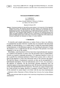
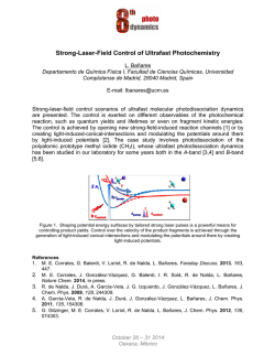

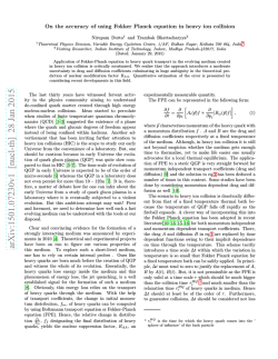
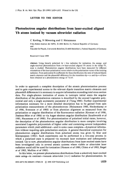
© Copyright 2026