
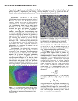
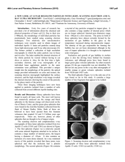
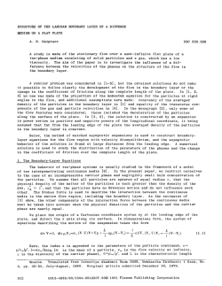
Improved Incompressible Smoothed Particle
Comput. Methods Appl. Mech. Engrg. 200 (2011) 1008–1020
Contents lists available at ScienceDirect
Comput. Methods Appl. Mech. Engrg.
journal homepage: www.elsevier.com/locate/cma
Improved Incompressible Smoothed Particle Hydrodynamics method
for simulating flow around bluff bodies
Mostafa Safdari Shadloo, Amir Zainali, Samir H. Sadek, Mehmet Yildiz ⇑
Faculty of Engineering and Natural Sciences, Advanced Composites and Polymer Processing Laboratory, Sabanci University, 34956 Tuzla, Istanbul, Turkey
a r t i c l e
i n f o
Article history:
Received 19 March 2010
Received in revised form 14 September 2010
Accepted 1 December 2010
Available online 7 December 2010
Keywords:
Meshless methods
Incompressible Smoothed Particle
Hydrodynamics (ISPH)
Airfoil problem
Square obstacle problem
Bluff body
Solid boundary treatment
a b s t r a c t
In this article, we present numerical solutions for flow over an airfoil and a square obstacle using Incompressible Smoothed Particle Hydrodynamics (ISPH) method with an improved solid boundary treatment
approach, referred to as the Multiple Boundary Tangents (MBT) method. It was shown that the MBT
boundary treatment technique is very effective for tackling boundaries of complex shapes. Also, we have
proposed the usage of the repulsive component of the Lennard-Jones Potential (LJP) in the advection
equation to repair particle fractures occurring in the SPH method due to the tendency of SPH particles
to follow the stream line trajectory. This approach is named as the artificial particle displacement method.
Numerical results suggest that the improved ISPH method which is consisting of the MBT method, artificial particle displacement and the corrective SPH discretization scheme enables one to obtain very stable and robust SPH simulations. The square obstacle and NACA airfoil geometry with the angle of attacks
between 0° and 15° were simulated in a laminar flow field with relatively high Reynolds numbers. We
illustrated that the improved ISPH method is able to capture the complex physics of bluff-body flows naturally such as the flow separation, wake formation at the trailing edge, and the vortex shedding. The SPH
results are validated with a mesh-dependent Finite Element Method (FEM) and excellent agreements
among the results were observed.
Ó 2010 Elsevier B.V. All rights reserved.
1. Introduction
Smoothed Particle Hydrodynamics (SPH) is one of the members
of meshless Lagrangian particle methods used to solve partial
differential equations widely encountered in scientific and engineering problems [1–4]. Unlike Eulerian (mesh-dependent) computational techniques such as finite difference, finite volume and
Finite Element Methods, the SPH method does not require a grid,
as field derivatives are approximated analytically using a kernel
function. In this technique, the continuum or the global computational domain is represented by a set of discrete particles. Here, it
should be noted that the term particle refers to a macroscopic part
(geometrical position) in the continuum. Each particle carries
mass, momentum, energy and other relevant hydrodynamic properties. These sets of particles are able to describe the physical
behavior of the continuum, and also have the ability to move under
the influence of the internal/external forces applied due to the
Lagrangian nature of SPH. Although originally proposed to handle
cosmological simulations [5,6], the SPH method has become
increasingly generalized to handle many types of fluid and solid
mechanics problems [7–11].
⇑ Corresponding author.
E-mail address: [email protected] (M. Yildiz).
0045-7825/$ - see front matter Ó 2010 Elsevier B.V. All rights reserved.
doi:10.1016/j.cma.2010.12.002
Due to being a relatively new computational method for engineering applications (roughly two decades old), there are still a
few significant issues with SPH that need to be scrutinized. It is still
a challenge to model physical boundaries correctly and effectively.
In addition, there are various ways to construct SPH equations (discretization), and a consistent approach has not gained consensus.
Highly irregular particle distributions which occur as the solution
progresses may cause numerical algorithms to break down, thereby making robustness another significant issue to be addressed.
Namely, it is well-known by SPH developers that when passing
from one test case to another, new problems are faced. For example, instabilities due to clamping of SPH particles which is not in
general present in modeling a dam-breaking problem show themselves in the simulation of flow over bluff bodies, especially at the
leading and trailing edges. These shortcomings are not insurmountable. The underlying factors causing these shortcomings
can be understood through extensive research on the verification
of SPH against a wide variety of possible applications as being done
in the SPH literature.
In most engineering problems, the domain of interest has, in
general, solid boundaries. The SPH formulations being valid for
all interior particles are not necessarily accurate for particles close
to the domain boundary since the kernel function is truncated by
the boundary. Therefore, the application of boundary conditions is
M.S. Shadloo et al. / Comput. Methods Appl. Mech. Engrg. 200 (2011) 1008–1020
problematic in the SPH technique. Consequently, the proper and
correct boundary treatments have been an ongoing concern for
an accurate and successful implementation of the SPH approach
[12,13] as well as other meshless methods [14,15] in the solution
of engineering problems with solid walls. Improper boundary
treatment has two important consequences. The first originates
from the penetration of fluid particles into boundary walls, which
then leave the computational domain. The second is that kernel
truncation at the boundary produces errors in the solution. Hence,
over the years, several different approaches have been used for
the boundary treatment such as specular reflections, or bounceback of fluid particles with the boundary walls [16], LennardJones Potential (LJP) type force as a repulsive force [17,18], ghost
particles [19–21], and Multiple Boundary Tangent (MBT) method
[22].
Additionally, the homogeneity of the particle distribution is
quite important for the accuracy and the robustness of SPH models.
The formation of ill particle distributions during the simulation
may result in the numerical solution to fail. For instance, if the
pressure field is solved correctly thereby imposing the incompressibility condition as accurately as possible, the particle motion closely follows the trajectory of streamline, hence resulting in a linear
clustering and in turn fracture in particle distribution. In these regions due to the lack of sufficient number of particles, or inhomogeneous particle distribution, the gradients of field variables can
not be computed reliably. Such a situation leads to spurious fields,
especially erroneous pressure values in the ISPH approach. As the
computation progresses, errors in computed field variables accumulate whereby blowing-up the simulation.
This paper suggests an improved ISPH algorithm that includes
the implementation of (i) the multiple boundary tangent method
to treat geometrically complex solid boundaries in a flow field,
(ii) the artificial particle displacement (particle fracture repair)
procedure for eliminating particle clustering induced instabilities,
and (iii) the corrective SPH discretization scheme to improve the
accuracy of the computation.
2. Smoothed Particle Hydrodynamics
For clarity of the presentation, it is worthy of introducing notational conventions to be used throughout this article. All vector and
tensorial quantities are written either using suffix notation with
Latin indices denoting the components or direct notation with
boldface letters. These components will be written either as subscripts (when particle identifiers are not used) or superscripts
(when particle identifiers are used). As well, throughout this article
the Einstein summation convention is employed, where any
repeated component index is summed over the range of the index.
These superscripts do not represent any covariant or contravariant
nature. Latin boldface indices (i, j) will be used as particle identifiers to denote particles and will always be placed as subscripts that
are not summed, unless indicated with a summation symbol. For
example, the position vector for particle i is ~
ri ¼ xki ~
ek where xki
denotes the components of the position vector and ~
ek is a base
vector. The distance
vector
between a pair of particles is indicated
ek ¼ r kij~
by ~
rij ¼ ~
ek , and the magnitude of the
ri ~
rj ¼ xki xkj ~
distance vector k~
rij k is denoted by rij.
The three-dimensional Dirac-delta function d3(rij), also referred
to as a unit pulse function, is the starting point for the SPH technique. This function satisfies the identity
f ð~
ri Þ ¼
Z
3
f ð~
rj Þd3 ðr ij Þd ~
rj ;
ð1Þ
X
3
rj is a differential volume element and X represents the towhere d ~
tal bounded volume of the domain.
1009
The SPH approach assumes that the fields of the particle of
interest are affected by that of all other particles within the global
domain. The interactions among the particles within the global domain are achieved through a compactly supported, normalized and
even weighting function (smoothing kernel function) W(rij, h) with
a smoothing radius jh (cut off distance, localized domain) beyond
which the function is zero. Hence, in computations, a given particle
interacts with only its nearest neighbors contained in this localized
domain. Here, the length h defines the support domain of the particle of interest, j is a coefficient associated with the particular kernel function, and rij is the magnitude of the distance between the
particle of interest i and its neighboring particles j. If the Dirac delta function in Eq. (1) is replaced by the kernel function W(rij, h), the
integral estimate or the kernel approximation to an arbitrary function f ð~
ri Þ can be introduced as
f ð~
ri Þ ffi hf ð~
ri Þi Z
3
f ð~
rj ÞWðrij ; hÞd ~
rj ;
ð2Þ
X
where the angle bracket h i denotes the kernel approximation, and ~
ri
is the position vector defining the center point of the kernel
function.
Approximation to the Dirac-delta function by a smoothing kernel function is the origin of the Smoothed Particle Hydrodynamics.
The Dirac-delta function can be replaced by a smoothing kernel
function provided that the smoothing kernel satisfies the following
several conditions; namely, (i) normalization condition: the area under the smoothing function must be unity over its support domain,
R
3
~
X Wðr ij ; hÞd rj ¼ 1, (ii) the Dirac-delta function property: as the
smoothing length approaches to zero, the Dirac-delta function
should be recovered, limh?0 W(rij, h) = d3(rij), (iii) compactness property: which necessitates that the kernel function be zero beyond its
compact support domain, W(rij, h) = 0 when rij > jh, and (iv) the
kernel function should be spherically symmetric even function,
W(rij, h) = W(rij, h), and be positive within the support domain
W(rij, h) > 0 when rij < jh. Finally, the value of the smoothing function should decay with increasing distance away from the center
particle.
The smoothing function can be represented in a general form as
W(rij, h) = (1/hd)f(rij/h) where d is the dimension of the problem,
and f is a function. In literature, it is possible to find a wide variety
of kernel functions which satisfy above-listed conditions, such as
Gaussian, cubic or quintic kernel functions [18,23]. The smoothing
kernels can be considered as discretization schemes in mesh
dependent techniques such as finite difference and volume. The
stability, the accuracy and the speed of an SPH simulation heavily
depend on the choice of the smoothing kernel function as well as
the smoothing length. Considering the stability and the accuracy
of the simulations, throughout the present work, the compactly
supported two-dimensional quintic spline kernel is used at the expense of higher computational cost. For example, the utilization of
the higher order quintic spline in simulations is at least two times
computationally more expensive than that of the cubic spline
8
ð3 sij Þ5 6ð2 sij Þ5 þ 15ð1 sij Þ5 if 0 6 sij < 1;
>
>
>
>
5
5
<
7
if 1 6 sij < 2;
ð3 sij Þ 6ð2 sij Þ
Wðrij ; hÞ ¼
2>
5
478ph >
ð3
s
Þ
if 2 6 sij 6 3;
ij
>
>
:
0
if sij P 3;
ð3Þ
here sij = rij/h. The spatial resolution of SPH is affected by the
smoothing length. Hence, depending on the problem solved, each
particle can be assigned to a different value of smoothing length.
However, for a variable smoothing length, it is probable to violate
Newton’s third law. For example, it might be possible for a particle
j to exert a force on particle i, and not to experience an equal and
opposite reaction force from particle i. To ensure that Newton’s
1010
M.S. Shadloo et al. / Comput. Methods Appl. Mech. Engrg. 200 (2011) 1008–1020
third law is not violated and the pair wise interaction among particles moving close to each other is achieved, the smoothing length is
substituted by its average, defined as hij = 0.5(hi + hj). The averaged
smoothing length ensures that particle i is within the influence domain of particle j and vice versa.
2.1. Spatial derivatives and particle approximation in SPH
The SPH approximation for the gradient of an arbitrary function
(i.e., scalar, vectorial, or tensorial) can be simply written through
the substitution f ð~
rj Þ ! @f ð~
rj Þ=@xkj in Eq. (2) to produce
@f ð~
ri Þ
ffi
@xki
*
+ Z
@f ð~
rj Þ
@f ð~
ri Þ
3
Wðr ij ; hÞd ~
rj :
k
@xki
X @xj
ð4Þ
Upon integrating Eq. (4) by parts and using the compactness property of the kernel function as well as noting that @Wðr ij ; hÞ=@xki ¼
@Wðrij ; hÞ=@xkj for a constant smoothing length h, it can be shown
that
*
+ Z
@Wðr ij ; hÞ 3
@f ð~
ri Þ
@f ð~
ri Þ
ffi
f ð~
rj Þ
d~
rj :
@xki
@xki
@xki
X
ð5Þ
Using a Taylor series expansion and the properties of a second-rank
isotropic tensor, as derived in Appendix A, a more accurate SPH
approximation for the gradient of an arbitrary function can be introduced as
N
X
r pij @Wðr ij ; hÞ
mj p
@ 2 f m ð~
ri Þ
p ~
~
¼
8
ðf
ð
r
Þ
f
ð
r
ÞÞ
;
i
j
qj
@xm
r 2ij
@xki @xki
i
j¼1
N
X
r sij @Wðr ij ; hÞ
mj p
@ 2 f p ð~
ri Þ
¼2
ðf ð~
ri Þ f p ð~
rj ÞÞ 2
:
k
k
q
@xsi
r ij
@xi @xi
j
j¼1
ð6Þ
PN
k
s
where aks
j¼1 ðmj =qj Þr ji ð@Wðr ij ; hÞ=@xi Þ is a corrective secondij ¼
rank tensor. This form is referred to as the corrective SPH gradient
formulation that can be used to eliminate particle inconsistencies. It
should be noted that the corrective term aks
ij is ideally equal to
Kronecker delta dks for a continuous function. On using Kronecker
delta in Eq. (6), one can obtain the SPH gradient formulation of a
vector-valued function commonly seen in the SPH literature. It
should be noted that the corrective SPH formulation requires the
inversion of aks
ij , which might be singular for irregular and ill particle
distribution. We have not experienced any difficulties related to aks
ij
corrective tensor being singular for a wide variety of benchmark
problems solved (i.e., lid driven cavity, flow over backward facing
step, Taylor vortices, and bubble deformation). However, if such a
singularity problem exists for a given particle which can easily be
determined through monitoring whether the determinant of the
aks
ij is zero or not, the corrective SPH formulation on that particle
ks
should not be imposed through setting aks
ij ¼ d , thereby leading
to the utilization of the standard SPH discretization scheme.
Additionally, there are two main forms of the SPH approximation for the Laplacian of a vector-valued function [19,24]. For the
sake of completeness, we have in Appendix A shown that these
two forms can be derived from the SPH representation of the second order spatial derivative of a vector field @ 2 f p ð~
ri Þ=@xki @xli as
N
X
r pij @Wðr ij ; hÞ
mj p
@ 2 f p ð~
ri Þ pm
p ~
~
a
¼
8
ðf
ð
r
Þ
f
ð
r
ÞÞ
;
i
j
qj
@xm
r 2ij
@xki @xki ij
i
j¼1
ð7Þ
N
X
rsij @Wðrij ; hÞ
mj p
@ 2 f p ð~
ri Þ 2 þ allij ¼ 8
ðf ð~
ri Þ f p ð~
rj ÞÞ 2
:
k
k
qj
@xsi
rij
@xi @xi
j¼1
ð8Þ
Likewise, upon replacing the corrective second rank tensor in Eq. (7)
and its trace in Eq. (8) by Kronecker delta and its trace, respectively,
one can obtain the SPH Laplacian formulations of a vector-valued
function suggested by Clearly and Monaghan [24], and Morris
et al. [19], correspondingly
ð10Þ
Unlike Eq. (8), Eq. (7) can only be used for divergence free vectorvalued functions as shown in Appendix A.
Throughout this work, all modeling result are obtained with the
usage of corrective SPH discretization schemes since corrective
SPH formulations produce more accurate and stable results than
the standard SPH equations. We have also observed that Eq. (7)
performs better for the discretization of the Laplacian of velocity
fields than Eq. (8). Therefore, in all presented results, Eq. (7) is used
for the Laplacian of velocity, while Eq. (8) is used for the Laplacian
of pressure in the Poisson pressure equation.
2.2. Instabilities and their possible remedies in the SPH method
To prevent the particle clustering, the trajectory of particles can
be disturbed by adding relatively small artificial displacement drki
to the advection of particles computed by the solution of the
equation of motion. Recall the form of the Lennard-Jones Potential
(LJP)-type force used in the SPH literature as a repulsive force for
the solid boundary treatment,
F ki;LJP ¼
N
X
ðro =r ij Þn1 ðro =r ij Þn2
j¼1
N
mj p
@Wðr ij ; hÞ
@f p ð~
ri Þ ks X
aij ¼
ðf ð~
rj Þ f p ð~
ri ÞÞ
;
k
q
@xsi
@xi
j
j¼1
ð9Þ
br kij v 2max
r 2ij
;
ð11Þ
where F ki;LJP is the force per unit mass on fluid particle i due to the
neighbor particles j, n1 and n2 are constants, b is a problemdependent parameter, ro is the cutoff distance, and vmax is the
largest particle velocity in the system. In this work, vmax is set to
be equal to the absolute value of the maximum vx velocity. If the
second term (attractive interaction) on the right-hand side of LJP
force is neglected, and n1 = 2, and the force F ki;LJP , and vmax are
replaced by dr ki =ðDtÞ2 and rij/Dt, one can write the relationship
dr ki ¼ b
N rk
X
ij
j¼1
r 3ij
r 2o v max Dt;
ð12Þ
where drki is an artificial particle displacement vector.
P
Here, the cut-off distance can be approximated as r o ¼ Nj¼1 rij =N.
k
3
Given that rij =rij is an odd function with vanishing integral, one can
P
write Nj¼1 rkij =r 3ij ¼ 0 for a spherically symmetric particle distribution. However, if the particle distribution is asymmetric, and clusP
tered, the term Nj¼1 r kij =r 3ij – 0 is no longer equal to zero, whereby
implying the region with clustered particle distribution. The artificial particle displacement is only influential in the clustered region
and negligibly small in the rest of the computational domain due to
PN k 3
j¼1 r ij =r ij ffi 0 provided that the particle distribution is closely uniform. The offset vector d^rkii between the particle i and the center of
mass of its influence domain can be presented as
d^r kii ¼ xki ^xki ¼
N
X
rkij =N;
ð13Þ
j¼1
where xki and ^
xki are the coordinates of the particle i and the center
of mass for the influence domain of the particle i.
The comparison of the artificial particle displacement and offset
vectors implies that upon using the particle displacement vector in
the advection equation, the particle i moves towards the diluted
particle region (the region which is away from the center of mass).
Hence, the fractures in the simulation domain are repaired. Since
the near boundary fluid particles have influence domains truncated
by boundaries, with the usage of the artificial particle displacement vector in the computation, these fluid particles will tend to
M.S. Shadloo et al. / Comput. Methods Appl. Mech. Engrg. 200 (2011) 1008–1020
move towards the boundary and stick to it. Even though this situation may appear as a problem and the deficiency of the approach,
it might be used in advantageous way such that fluid particles
close to boundaries are then artificially forced to move in conformation with boundaries. Hence pressure forces on the boundaries
can be computed much more accurately in that particle deficiency
is no longer problem therein. In our simulations, since the ghost
particles are used for near boundary fluid particles, the influence
domain of the kernel function is fully populated, and therefore
such a problem is not an issue. The artificial particle displacement
vector is added to the particle advection equation in both prediction and correction steps. This approach repairs all the clustering
and fracture in the domain gradually without inducing significant
errors in the computation, and enabling a quite robust SPH approach. It is due to this approach that it becomes possible to run
simulations with higher Reynolds numbers, which are otherwise
impossible to achieve.
2.3. SPH solution algorithms
The governing equations used to solve the fluid problems in this
article are the mass and linear momentum balance equations
which are expressed in the Lagrangian form and given in direct
notation as
Dq=Dt ¼ qr ~
v;
ð14Þ
qD~
v =Dt ¼ r r þ q~f B :
ð15Þ
In the present simulations, the fluid is assumed to be incompressible and Newtonian. Hence, the incompressibility condition requires
that the divergence of the fluid velocity r ~
v ¼ 0 be zero. Here, q is
the fluid density, ~
v is the divergence-free fluid velocity, r is the total
stress tensor, and ~
f B is the body force term, respectively. The total
stress is defined as r = pI + T, where p is the absolute pressure, I
is the identity tensor, T ¼ lðr~
v þ ðr~
vÞT Þ is the viscous part of the
total stress tensor, where l is the viscosity. Finally, D/Dt is the
material time derivative operator defined as D/Dt = @/@t + vl@/@xl.
There are two common approaches utilized in the SPH literature
for solving the balance of the linear momentum equation. The first
one is widely referred to as the Weakly Compressible SPH (WCSPH)
where the pressure term in the momentum equation is determined
through an artificial equation of state. In the second approach
known as the Incompressible SPH (ISPH), the pressure is computed
by means of solving a pressure Poisson equation.
The ISPH approach is based on the projection method [25–27],
which uses the principle of Hodge decomposition. Upon using the
Hodge decomposition, any vector field can be broken into a divergence-free part plus the gradient of an appropriate scalar potential.
The Hodge decomposition can be written for a velocity field as
~
v ¼ ~
v þ ðDt=qÞrp;
ð16Þ
where v is the intermediate velocity, and ~
v is the divergence-free
part of the velocity field. The projection method begins by ignoring
the pressure gradient in the momentum balance equation. The
solution of Eq. (15) without the pressure gradient produces the
intermediate velocity ~
v , which does not, in general, satisfy mass
conservation. However, this incorrect velocity field can be projected
onto a divergence-free space after solving a pressure Poisson equation, from which the divergence-free part of the velocity field ~
v can
be extracted. The pressure Poisson equation is obtained by taking
the divergence of Eq. (16) as
~
r~
v =Dt ¼ r ðrp=qÞ:
ð17Þ
Eq. (17) is subjected to Neumann boundary conditions that can be
obtained by using the divergence theorem on the pressure Poisson
equation as
ðq=DtÞ~
v ~
n ¼ rp ~
n;
1011
ð18Þ
where ~
n is the unit normal vector. Having solved the pressure Poisson equation to obtain the pressure field and then computed the
pressure gradient, we can use the Hodge decomposition equation
to determine the correct, incompressible velocity field ~
v . Often,
the boundary conditions for ~
v ðnþ1Þ are used for ~
v . This reduces Neumann boundary condition to rp ~
n ¼ 0 for no slip boundary condition. Note that in order for differentiating between spatial and
temporal indices, the time index n is put within brackets.
One of the main advantages of using ISPH is the elimination of
the speed of sound parameter in the time-step conditions. Much
larger time steps can be used in this approach, at the computational expense of having to solve the pressure Poisson equation
at each time step. The algorithm stability is controlled by the Courant–Friedrichs–Lewy (CFL) condition, where the recommended
time-step is Dt 6 CCFLhij,min/vmax where hij = 0.5(hi + hj), hij,min is
the minimum smoothing length among all i–j particle pairs, and
CCFL is a constant satisfying 0 < CCFL 6 1 (in this work, CCFL = 0.125).
For time marching of the ISPH approach, we have used a firstorder Euler time step scheme. This technique is an explicit time
integration scheme, and is relatively simple to implement. Particle
positions, and velocities are computed respectively as D~
ri =Dt ¼
~
vi ; D~
vi =Dt ¼ ~f i . The general form of the ISPH algorithm is as follow. The predictor step starts with determining an estimate ~
ri for
ðnÞ
all particle locations, given the previous particle positions ~
ri and
ðnÞ
the previous correct velocity field ~
v ðnÞ
as ~
ri ¼ ~
ri þ ~
v ðnÞ
Dt where
i
i
~
ri is the intermediate particle position. The intermediate velocity
field ~
v i is computed on the temporary particle locations through
the solution of the momentum balance equations with forward
time integration by omitting the pressure gradient term as
~ðnÞ
~
vi ¼ ~
v ðnÞ
i þ f i Dt. The pressure Poisson equation is solved to obtain
ðnþ1Þ
the pressure pi
which is required to enforce the incompressibility condition. The pressure Poisson equation is solved using a
biconjugate gradient stabilized method or a direct solver based
on the Gauss elimination method. The Hodge decomposition principle is employed to solve for the actual velocity field ~
v ðnþ1Þ
by
i
ðnþ1Þ
using the computed pressure pi
. Finally, with the correct velocity field for time-step n + 1, all fluid particles are advected to their
ðnþ1Þ
new positions ~
ri
using an averageof the previous
and current
ðnþ1Þ
ðnÞ
~ðnþ1Þ Dt.
particle velocities as ~
ri
¼~
ri þ 0:5 ~
v ðnÞ
i þ vi
2.4. Mesh generation and MBT boundary treatment for airfoil
geometry
This section presents the geometry and mesh generation, ghost
particle creations and the implementation of the MBT boundary
treatment for the airfoil geometry. Initially, a Cartesian mesh is
created over a rectangular domain with the length and height of
L and H, respectively. Then, an airfoil geometry is created using
Eqs. (20) and (21). Since the leading edge of the airfoil has a curve
with a steeper slope, the chord is split into two parts to be able to
locate more boundary particles towards the leading edge. Discrete
points on the chord are created with the formula
xc ¼ ½ði 1Þ=ðilen 1Þn idis
ð19Þ
where xc is coordinates along the chord of the airfoil, i is a nodal index, ilen is the number of nodes along the chord, idis is the length of
the chord, and n is the geometrical progression coefficient which
controls the distance between points on the chord. Given the chord
length of 1, 6 inequidistant nodal points created through the geometrical progression coefficient of 2 are located along the 5% of
the chord length starting from the leading edge. The remaining section of the chord has 50 equidistant nodal points. The mean camber
line coordinates are computed using Eq. (20)
1012
yc ¼ m 2pxc x2c =p2
yc ¼ mð2pðxc 1Þ þ 1 x2c Þ=ð1 p2 Þ
M.S. Shadloo et al. / Comput. Methods Appl. Mech. Engrg. 200 (2011) 1008–1020
0 6 xc 6 p;
p < xc 6 1;
ð20Þ
where m is the maximum camber in percentage of the chord, which
is taken to be 5%, p is the position of the maximum camber in percentage of the chord that is set to be 50%, and t is the maximum
thickness of the airfoil in percentage of the chord, which is 15%.
The thickness distribution above and below the mean camber line
is calculated as
2
3
4
yt ¼ 5t 0:2969x0:5
c 0:126xc 0:3516xc þ 0:284xc 0:1015xc :
ð21Þ
The final coordinates of the airfoil for the upper surface (xU, yU) and
the lower surface (xL, yL) are determined using the following
relations: xU = xc ytsinu, yU = yc + ytcosu, xL = xc + ytsinu, yL = yc ytcosu, and u = arctan(dyc/dx). Having obtained all coordinates of
the airfoil geometry, the upper and lower surface lines are curve fitted using the least square method of order six. In so doing, it becomes possible to compute boundary unit normals, tangents and
slopes for each boundary particles. All the initial particles falling
between the upper and lower camber fitted curves are removed
from the rectangular computational domain, then remaining fluid
particles are combined with the boundary particles to form a particle array of the computational domain.
The various steps of implementing the MBT boundary treatment technique to the airfoil geometry, as depicted in Figs. 1 and
2, are as follows:
(a) At each or prescribed time steps, all near boundary fluid particles (particles with boundary truncations) as well as
boundary particles are associated with their neighbor boundary particles using the cell array data structure (the Fortran
90 derived data type) as also described in our earlier work
[22], see Fig. 1a. When dealing with a thin solid object
enclosed by flow such as the trailing edge of the airfoil, for
instance, near boundary fluid particles or boundary particles
positioned above/on the upper camber take contribution
from fluid and boundary particles located below the upper
camber since the weighting function W(rij, h) has an influence domain that spans over the smoothing radius jh. Physically, particles flanking a solid wall should not affect each
other. Consequently, the neighbor list computed through
the standard box-sorting algorithm has to be modified, and
then updated at each time step. The neighbor boundary particles of a given near boundary fluid particle are sorted in
accordance with the distance between boundary particles
and the fluid particle in ascending order. Then, the fluid particle in question is given the unit normal vector of its nearest
boundary neighbor particle. For instance, fluid particle i = 25
in Fig. 1a is given the unit normal of the boundary particle
i = 7. The neighbor lists of all particles are updated by computing the angles ð~
ni ~
nj Þ among unit normal vectors of particles and their neighbors. Here, ~
ni and ~
nj are the unit
normal of a given particle and its neighbors. Only the particles with angles smaller than the preset value (130° used in
this study) are regarded as neighbors to each other, whereby
forming the updated neighbor list. To be more specific, as
can be seen from Fig. 1b, the updated neighbor list of the
particle i = 25 includes only those particles enclosed by a
square frame since other neighbor particles do not satisfy
the preset angle condition even though they are in the influence domain of the particle i = 25.
(b) As in the case of step-a, all near boundary fluid and boundary particles are associated with their updated neighbor
boundary particles. Associating near boundary fluid particles
and boundary particles with their neighbor boundary particles, and sorting and then storing these neighbor boundary
particles in accordance with the shortest distance among
them allows for (i) the computation of the overlapping contributions of mirrored particles from each boundary particle,
(ii) the confinement of the mirrored particles into the solid
domain, (iii) defining solid boundaries by the envelope of
boundary tangent lines, as well as (iv) associating mirrored
particles with near boundary fluid particles.
(c) Given that each boundary particle has fluid particles in its
influence domain as neighbors, these fluid particles are mirrored with respect to the tangent line of the corresponding
boundary particle as indicated in Fig. 2. The fluid particles
should satisfy the condition ~
rbf ~
nb P 0, where ~
rbf is a position vector between the boundary particle and its neighbor
fluid particles directing towards the fluid particles and ~
nb
is the unit normal of the boundary particle. This condition
ensures that only fluid particles above the associated boundary particle tangent line are mirrored. The second condition
~
rnbg ~
nnb 6 0 to be fulfilled is that mirrored particles should
be confined into the solid region, meaning that mirrored
Fig. 1. Boundary treatment for a submerged thin object: step-a.
M.S. Shadloo et al. / Comput. Methods Appl. Mech. Engrg. 200 (2011) 1008–1020
1013
Fig. 2. Boundary treatment for a submerged thin object; (a) step-c and (b) step-d.
particles associated with a boundary particle have to be
inside of the all tangent lines of the neighbor boundary particles of the boundary particle in question, where ~
rnbg is the
position vector between the ghost particles and the neighbor
boundary particles of the given boundary particle and, ~
nnb is
the unit normal vector of the neighbor boundary particles
for the boundary particle in question. Using the cell array
structure, every boundary particle is associated with its corresponding mirrored particles. Spatial coordinates and particle identification numbers of mirrored particles are stored in
a cell array. To be more precise, mirrored particles are associated with the particle identification number of the fluid
particle from which they are originated (referred to as the
‘mother’ fluid particle). For example, for a fluid particle
indexed with i = 25, the ghost particle mirrored about a
boundary particle tangent line (for example, boundary particle 7) will also be associated with i = 25 as shown in Fig. 2a.
Note that fluid and boundary particles have numerical identifications that are permanent, whereas mirrored particles
have varying (dummy) indices throughout the simulation.
A ghost particle is given the same mass, density and transport parameters, such as viscosity, as the corresponding fluid
particle. As for the field values (i.e. velocities) of a ghost particle, they are obtained depending on the type of boundary
condition implemented. For instance, for no-slip boundary
conditions, the following relation is implemented: ~
vg ¼
2~
vb ~
v f where ~
vg ; ~
v b and ~
v f are the velocities of the ghost,
boundary, and fluid particles, respectively. As for the implementation of a zero-gradient at the boundary, a ghost particle is given the same field values as the corresponding fluid
particle; ~
vg ¼ ~
v f , and pg = pf, where pg and pf are the pressures of the ghost and fluid particles. If the boundaries are
stationary walls, the ghost particles will have the velocity
~
v g ¼ ~
v f for no-slip boundary conditions.
(d) In a loop over all particles, if a fluid particle has a boundary
particle or multiple boundary particles as neighbor(s), then
the fluid particle will become a neighbor of all mirrored particles associated with the corresponding boundary particles
on the condition that (i) the mirrored particles are in the
influence domain of the fluid particle in question, and (ii)
for a mirrored particle, its mother particle has to be within
the influence domain of the fluid particle in question. During
the creation of ghost particles, there is an over-creation of
ghost particles due to the fact that the influence domain of
neighboring boundary particles overlaps. The overlapping
contributions of mirrored particles can be eliminated by
determining the number of times a given fluid particle is
mirrored into the influence domain of the associated fluid
particle with respect to a boundary particle’s tangent line.
For computational efficiency, the fluid particle might only
be associated with the mirror particles of its several nearest
boundary particle rather than all neighbor boundary particles as explained in Fig. 2b. Boundary particle i = 7 has the
shortest distance to i = 25 compared to other boundary particles neighbor to the fluid particle i = 25. Hence, mirror particles of i = 7 also become the neighbor of i = 25 provided
that above two conditions (i and ii) are satisfied. Near
boundary fluid particles hold the information of spatial coordinates and fluid particle identity numbers, boundary particle identity numbers (i.e. the particle number for a boundary
particle to which mirrored particles are associated initially),
and over-creation number for mirrored particles in the cell
array format. During the SPH summation over ghost particles for a fluid particle with a boundary truncation, the mass
of the ghost particles are divided by the number of corresponding over-creations.
3. Flow around a square obstacle and an airfoil
In this work, to be able to test the effectiveness of the improved
SPH algorithm proposed in Section 2 (involving the utility of the
MBT method together with the artificial particle displacement
and the corrective SPH discretization scheme) for modeling fluid
flow over complex geometries, we have solved two benchmark
flow problems; namely, two-dimensional simulations of a flow
around a square obstacle and a NACA airfoil. Mass and linear
momentum balance equations are solved for both test cases on a
rectangular domain with the length of L = 15 m and the height of
H = 6 m.
A square obstacle with a side dimension of 0.7 m is positioned in
the computational domain with its center coordinates at x = L/3 and
y = L/2. Initially, a 349 145 array (in x- and y-directions, respectively) of particles is created in the rectangular domain, and then
particles within the square obstacle are removed from the particle
1014
M.S. Shadloo et al. / Comput. Methods Appl. Mech. Engrg. 200 (2011) 1008–1020
array. This set of initial particles are created regularly through the
formulations x = (i 1) L/(ilen 1), and y = (j 1) H/(jlen 1)
where x and y are coordinates of particles, i and j are nodal indices
in the x- and y-directions, respectively, and ilen and jlen are the
number of nodes along the x- and y-directions in the given order.
The boundary particles on the square obstacle are created such that
their particle spacing is almost the same as the initial particle spacing of the fluid particles. The implementation of the MBT method
for the square obstacle follows the same steps described previously
for the airfoil geometry. The simulation parameters, fluid density,
dynamic viscosity and body force are taken as respectively
q = 1000 kg/m3, l = 1 kg/ms, and F xB ¼ 3:0 103 N=kg. The mass
of each particle is constant and found through the relation
P
mi = qi/ni where ni ¼ j¼1 Wðr ij ; hÞ is the number density of the particle i. The smoothing length for all particles is set equal to 1.6 times
the initial particle spacing.
The slightly modified periodic boundary condition is implemented for inlet and outlet particles in the direction of the flow.
Particles crossing the outflow boundary are reinserted into the
flow domain at the inlet from the same y-coordinate positions with
the velocity of inlet fluid region with its coordinates of x = 0, and
y = 3 so that the inlet velocity profile is not poisoned by the outlet
velocity profile. The no-slip boundary condition is implemented for
Fig. 3. A close-up view for particle positions around the square obstacle for
Reynolds number of 300.
the square obstacle. For upper and lower walls bounding the simulation domain, the symmetry boundary condition for the velocity
is applied such that vy = 0, and @vx/@y = 0 which is discretized by
using Eq. (6). As for the pressure, a zero-pressure gradient condition rp ~
n ¼ 0 is enforced on all solid boundary particles.
The channel geometry and the boundary conditions for the second benchmark problem are identical to the first one except that
the square obstacle geometry is replaced by the NACA airfoil with
a chord length of 2 m. The leading edge of the airfoil is located at
Cartesian coordinates (L/5, H/2). Initially, a 300 125 array (in
x- and y-directions, respectively) of particles is created in the rectangular domain, and then, particles within the airfoil are removed
from the particle array. Subsequently, boundary particles are created and then distributed on solid boundaries. The smoothing
length for all particles is set equal to 1.6 times the initial particle
spacing. To show convergence, we run a test case with three different particle arrays, namely, 150 62, and 300 125 and
400 167 were used. It was observed that 300 125 array of particles is sufficient for particle number independent solutions.
The flow around the airfoil and square obstacle positioned inside the channel were simulated for a range of Reynolds numbers
Re = qlcvb/l, which is defined by the characteristic length, lc (set
equal to the side length for the square obstacle, and the chord
length for the airfoil geometry), the density, the bulk flow velocity
vb and the dynamic viscosity l. Both test cases are validated
through comparing SPH results with those obtained by a Finite
Element Method (FEM) based solver of a Comsol multiphsics
software tool. The ISPH and FEM results are compared in terms
of velocity contours for both test cases, and the pressure envelope
for the airfoil.
Fig. 3 shows the close-up view of particle positions around the
square obstacle for Reynolds number of 300. One can conclude that
the implementation of the MBT method together with the artificial
particle displacement and the corrective SPH discretization scheme
can successfully hinder the formation of chaotic particle distribution and fracture (unlike those observed in Ref. [22]) in the entire
flow domain (particularly in the vicinity of the boundary) and
effectively prevent the particle penetration through the boundary
(see Fig. 3), whereby producing simulation results in excellent
agreement with FEM method as shown in Fig. 4. It is noted that
Fig. 4. A comparison of ISPH (left) and FEM (right) velocity contours for two different Reynolds number values, 100 and 200. It should be noted that in this presentation, all
velocities are given as a velocity magnitude.
M.S. Shadloo et al. / Comput. Methods Appl. Mech. Engrg. 200 (2011) 1008–1020
for all of the test cases, the artificial particle movement coefficient
is kept constant and equal to 0.01. It is also noted that this coefficient should be selected carefully such that it should be small enough not to affect the physics of the flow, but also large enough to
prevent the occurrence of clustering and particle deficiency. Fig. 4
compares ISPH and FEM velocity contours for two different Reynolds number values, 100 and 200.
It is well-known from both earlier experiments and numerical
studies that vortex shedding is observed at the rear edge of the
square obstacle at higher Reynolds numbers [28]. In light of this,
to be able address whether the SPH method can capture vortex
shedding as accurately as mesh dependent solvers, we here present
simulation results for Reynolds number of 300, where Fig. 5 (left
figures) shows the simulation results for the vortex tail down
and up. On comparing ISPH and FEM results, one can notice that results are satisfactorily in agreement with each other regarding the
magnitude of velocities as well as the position and the number of
vortices. However, there is a slight discrepancy between ISPH and
FEM results in terms of the separation point of the vortices from
the rear edge of the obstacle. For the sake of brevity, without presenting further results, we can safely assert that the SPH method is
highly successful in predicting changes of the topology of the vortex shedding behind a square obstacle with the Reynolds number.
To have a closer look at the vortex shedding behavior captured
at the trailing edge of the square obstacle by the ISPH method, in
Fig. 6 are presented the streamlines of vortex shedding for a full
period for the Reynolds number of 300. One can immediately notice the development of a small vortex at the rear top edge of the
square obstacle, which is growing in size during its motion towards
the rear lower edge, and then separating from therein. The next
vortex starts at the lower rear edge, and grows in size while moving towards the top rear edge, and finally leaves the top rear edge.
The accuracy of the ISPH method can be further validated by
considering the Strouhal number, which is defined as St = xlc/vb,
where x is the frequency of vortex shedding. The computed value
of the Strouhal number for the ISPH method for the Reynolds number of 300 is 0.142, which is also consistent with the experimental
result reported in the literature [29].
Having showed the capability and effectiveness of the improved
ISPH algorithm on a geometry with sharp corners, we further
tested our algorithm on a more general and complex geometry
with curved boundaries and a thin body section. Fig. 7 presents a
close-up view of particle positions around airfoils with the angles
1015
of attack of 5° and 15° for a simulation time of 100 s, corresponding
to the Reynolds number of 570.
The proposed algorithm is also very successful in simulating the
flow around the airfoil geometry with any geometrical orientations
across the flow field, whereby producing simulation results in very
good agreement with the FEM method as shown in Figs. 8 and 9.
Fig. 8 compares SPH and FEM velocity contours for the angle of attack of 15° with the Reynolds number value of 570.
The pressure envelope results obtained by ISPH and FEM for
smaller angles of attack are also in very good agreement with each
other with some local deviations as shown in Fig. 9 (left). As for the
angle of attack of 15°, there is a slight departure in pressure values
from FEM results for the upper camber in the vicinity of leading
edge and the stagnation point. These discrepancies in pressure values might be attributed to the dynamic nature of the SPH method
since fluid particles are in continuous motion. Hence, there might
be a local temporary depletion of particles nearby the solid boundaries as shown in Fig. 7, which deteriorates the accuracy of the
computed pressure because the SPH gradient discretization
scheme is rather sensitive to the particle deficiencies within the
influence domain of the smoothing kernel function. Except the local deviations in pressure values on the airfoil, SPH results compare
excellently well with FEM solutions. Additionally, the pressure differences between upper and lower camber which correlate with
the lift force are in match with FEM results for a given position
on the boundary.
In order to investigate the sensitivity of the numerical solutions
to particle numbers in the ISPH method and the underlying mesh
in FEM, the velocity field over the airfoil at the same values of
the parameters have been computed on three different sets of particles (i.e., 150 62 (coarse), 300 125 (intermediate), and
400 167 (fine)) and two sets of meshes (i.e., 11,953 number of
triangular elements with 54,688 degrees of freedom (DOF)
(coarse), and 191,248 number of triangular elements with
864,206 DOF (fine)). Fig. 10 shows velocity contours in terms of
velocity magnitudes for the airfoil with the angle of attack of 15°
at Reynolds number of 420. The comparison of results on the
coarse, medium and the fine particle numbers demonstrates evidently that the intermediate particle number provides solutions
with sufficient accuracy considering the trade-off between computational costs and capturing the features being studied. Since finer
meshes are computationally expensive, the intermediate particle
number is chosen for the numerical simulations presented in this
Fig. 5. The comparison of vortex shedding contours obtained with ISPH (left) and FEM (right) methods for the cases of vortex tail down (up figures) and up (down figures) for
the Reynolds number of 300.
1016
M.S. Shadloo et al. / Comput. Methods Appl. Mech. Engrg. 200 (2011) 1008–1020
Fig. 6. The streamlines of vortex shedding for a full period at the Reynolds number of 300 plotted on particle distribution where colors denote the velocity magnitude. One
period T is 9.85 s. (For interpretation of the references to color in this figure legend, the reader is referred to the web version of this article.)
article. The simulations are performed on a workstation with
the configuration of Intel (R) Core (TM) i7 (@9500 @3.07 GHz)
processor under Windows XP (64 bit) operating system. The
computational cost in terms of CPU time for the coarse, medium
and fine particle numbers are 1.36, 3.24 and 14.05 s per each time
step, respectively.
M.S. Shadloo et al. / Comput. Methods Appl. Mech. Engrg. 200 (2011) 1008–1020
1017
Fig. 7. Close-up view of particle positions around airfoils with the angles of attack of 5° and 15° for a simulation time of 100 s, corresponding to the Reynolds number of 570.
For the angle of attack of 15°, there is slight particle depletion in the close vicinity of the stagnation point, which is not observed for lower values of the angle of attack.
Fig. 8. A comparison of ISPH (left) and FEM (right) velocity contours for the angle of attack of 15° with the Reynolds number value of 570.
Fig. 9. The comparison of pressure envelopes for the angles of attack of 5° (left) and 15° (right) for the Reynolds numbers of 420 (up) and 570 (down).
1018
M.S. Shadloo et al. / Comput. Methods Appl. Mech. Engrg. 200 (2011) 1008–1020
Fig. 10. The velocity fields in terms of velocity magnitudes over the airfoil (with the angle of attack of 15° at Reynolds number of 420) computed on three different sets of
particles for the ISPH method and on two sets of meshes for FEM.
Fig. 11. The comparison of vortex shedding contours produced by ISPH (left) and FEM (right) methods for the angle of attack of 10° and the Reynolds number of 1600.
Fig. 11 compares ISPH and FEM results in terms of the vortex
shedding contours for the angle of attack of 10° with the Reynolds
number of 1600. As in the case of the presented square obstacle results, SPH results are also satisfactorily in agreement with FEM
regarding the magnitude of velocities as well as the position and
the number of vortices for the airfoil geometry.
The vortex shedding behavior computed by the SPH method is
presented in Fig. 12 as a close-up view magnifying the region about
one airfoil length behind the trailing edge in terms of the streamlines of vortex shedding for a full period for the Reynolds number
of 1400 and the angle of attack of 10°. There are two vortices near
the trailing edge of the airfoil, one being on the upper camber, and
the second is at the end of the trailing edge. The first vortex is
pushing the second vortex away from the trailing edge during its
downward motion towards the trailing edge. When the second
vortex disappears, and the first vortex reaches to the trailing edge,
a new vortex appears on the upper camber again, thereby completing a full period.
4. Conclusion
In this work, we have presented solutions for flow over an airfoil and a square obstacle using an improved ISPH algorithm that
can handle complex geometries with the usage of the MBT method,
and eliminate particle clustering induced instabilities with the
implementation of artificial particle displacement (particle fracture repair) procedure as well as the corrective SPH discretization
scheme. The close-up views for the distribution of fluid particles
around bluff bodies illustrate that the proposed boundary treatment prevents both particle deficiency and particle penetration
across the solid boundary without disturbing flow structure. We
have shown that the improved ISPH method can be effectively
1019
M.S. Shadloo et al. / Comput. Methods Appl. Mech. Engrg. 200 (2011) 1008–1020
Fig. 12. The streamlines of vortex shedding for a full period at the Reynolds number of 1400 plotted on particle distribution where colors denote the velocity magnitude. One
period T is 3.2 s. (For interpretation of the references to color in this figure legend, the reader is referred to the web version of this article.)
used for flow simulations over bluff-bodies with Reynolds numbers as high as 1600, which is not achievable with standard ISPH
formulations. It should be noted that the improved ISPH algorithm
is not limited to simulations for Reynolds numbers of 1600 in laminar flow regime. It can run to higher Reynolds number values
without any interruption. Our simulation results are validated with
an FEM method, and excellent agreements among the results were
observed. We illustrated that the improved ISPH method is able to
capture the complex physics of bluff-body flows naturally such as
flow separation, wake formation at the trailing edge, and vortex
shedding without any extra effort to increase the particle resolution in some specific areas of interest. As well, our future work includes the implementation of artificial particle displacement
algorithm for the flow problems with free surfaces as well as the
utilization of the MBT boundary treatment method in multiphase
flow problems.
Z
ðf p ð~
rj Þ f p ð~
ri ÞÞ
X
¼
@f p ð~
ri Þ
@xli
Funding provided by the European Commission Research Directorate General under Marie Curie International Reintegration Grant
program with the Grant Agreement number of 231048 (PIRG03GA-2008-231048) is gratefully acknowledged.
Appendix A
Ils
@Wðr ij ; hÞ 3
rlji r kji
d~
rj :
@xsj
X
|fflfflfflfflfflfflfflfflfflfflfflfflfflfflfflfflfflfflffl{zfflfflfflfflfflfflfflfflfflfflfflfflfflfflfflfflfflfflffl}
@f p ð~
ri Þ
f p ð~
rj Þ ¼ f p ð~
ri Þ þ r lji
@xli ~
rj ¼~
ri
1
@f p ð~
ri Þ
þ rlji r kji l k 2
@xi @xi ðA:2Þ
Ilks ¼0
Note that the first and the second integrals on the right hand side of
Eq. (A.2) are, respectively, second- and third-rank tensors. The
third-rank tensor Ilks can be integrated by parts, which, upon using
the Green–Gauss theorem produces Eq. (A.3) since the kernel
W(rij, h) vanishes beyond its support domain
Z
@ l k 3
r r d~
rj
@rsj ji ji
X
Z
3
¼ Wðr ij ; hÞ r lji dsk þ r kji dls d ~
rj
Wðr ij ; hÞ
ðA:3Þ
X
Recalling that the kernel function is spherically symmetric even
function and the multiplication of an even function by an odd function produces an odd function. Integration of an odd function over a
symmetric domain leads to zero
Ilks ¼ dsk
The following section provides derivations for the SPH approximation to first- and second-order derivatives of a vector-valued
function. The derivations are carried out in Cartesian coordinates.
The SPH approximation for the gradient of a vectorial function
starts with a Taylor series expansion of f p ð~
rj Þ so that
@Wðr ij ; hÞ 3
1 @f p ð~
ri Þ
d~
rj þ
s
l
k
2
@x
@x
@x
X
j
i
i
|fflfflfflfflfflfflfflfflfflfflfflfflfflfflfflfflffl{zfflfflfflfflfflfflfflfflfflfflfflfflfflfflfflfflffl}
rlji
Z
Ilks ¼ Acknowledgement
Z
@Wðr ij ; hÞ 3
d~
rj
@xsj
Z
Z
3
3
r lji Wðr ij ; hÞd ~
rj dls rkji Wðrij ; hÞd ~
rj ¼ 0:
X
X
|fflfflfflfflfflfflfflfflfflfflfflfflfflfflffl{zfflfflfflfflfflfflfflfflfflfflfflfflfflfflffl}
|fflfflfflfflfflfflfflfflfflfflfflfflfflfflffl{zfflfflfflfflfflfflfflfflfflfflfflfflfflfflffl}
¼0
ðA:4Þ
¼0
Following the above described procedure identically, the second
rank tensor Ils can be written as
Ils ¼ dls
Z
3
Wðr ij ; hÞd ~
rj ¼ dls :
|fflfflfflfflfflfflfflfflfflfflfflffl{zfflfflfflfflfflfflfflfflfflfflfflffl}
ðA:5Þ
X
:
ðA:1Þ
~
rj ¼~
ri
Upon multiplying Eq. (A.1) by the term, @Wðr ij ; hÞ=@xsj , and then
3
rj , one can write,
integrating over the whole space d ~
¼1
On combining Eq. (A.2) with Eqs. (A.4) and (A.5), one can write,
@f p ð~
ri Þ
¼
@xsi
Z
X
ðf p ð~
rj Þ f p ð~
ri ÞÞ
@Wðr ij ; hÞ 3
d~
rj :
@xsi
ðA:6Þ
1020
M.S. Shadloo et al. / Comput. Methods Appl. Mech. Engrg. 200 (2011) 1008–1020
Note that in Eq. (A.6), the relationship @Wðrij ; hÞ=@xsj ¼
@Wðrij ; hÞ=@xsi has been used. Replacing the integration in Eq.
(A.6) with the SPH summation over particle ‘‘j’’ and setting
3
d~
rj ¼ mj =qj , we can obtain the gradient of a vector-valued function
in the form of the SPH interpolation as
Upon contracting on indices s and m of Eq. (A.10), an alternative
form of the Laplacian for a vector field can be obtained as
N
mj p
@Wðr ij ; hÞ
@f p ð~
ri Þ X
¼
ðf ð~
rj Þ f p ð~
ri ÞÞ
:
s
@xi
qj
@xsi
j¼1
If the trace of the Kronecker delta in Eq. (A.15) is replaced by the
trace of Eq. (A.12), one can obtain an alternative form of the corrective SPH interpolation for the Laplacian.
ðA:7Þ
It is important to note that the second rank tensor Ils, shown to be
equal to Kronecker delta for a continuous function, may not be
equal to Kronecker delta for discrete particles. Hence, for the accuracy of the computations, this term should be included in the SPH
gradient interpolation of a function. From Eq. (A.2), we can write
N
X
mj
qj
j¼1
¼
ðf p ð~
rj Þ f p ð~
ri ÞÞ
@Wðr ij ; hÞ
@xsi
N
mj l @Wðrij ; hÞ
@f p ð~
ri Þ X
r
:
l
@xsi
@xi j¼1 qj ji
ðA:8Þ
Eq. (A.8) can be written in matrix form as
3 2
N
N
P
P
ð1Þ ð1Þ
ð1Þ ð1Þ
6 fji aj 7 6 r ji aj
7 6 j¼1
6 j¼1
7¼6
6
7 6 N
6P
4 N ð1Þ ð2Þ 5 4 P
ð1Þ ð2Þ
fji aj
r ji aj
3
2 ð1Þ 3
ð2Þ ð1Þ
r ji aj 7 @fið1Þ
76 @xi 7
j¼1
76
7
74 ð1Þ 5;
N
P
ð2Þ ð2Þ 5 @fi
r ji aj
ð2Þ
@x
2
j¼1
N
P
j¼1
ðA:9Þ
i
j¼1
where asj ¼ ðmj =qj Þ @Wðr ij ; hÞ=@xsi .
Starting with the relation for the SPH second-order derivative
approximation [22] of a vector valued-function f p ð~
ri Þ given in Eq.
(A.10)
2
Z
ðf p ð~
ri Þ f p ð~
rj ÞÞ
X
¼
rsij @Wðrij ; hÞ 3
d~
rj
@xm
r2ij
i
2 @ 2 f p ð~
ri Þ 1 @ 2 f p ð~
ri Þ sm
þ
d ;
s
k
k
n @xi @xm
n
@x
@x
i
i
i
ðA:10Þ
which, upon contracting on indices p and s, one can obtain
2
Z
ðf p ð~
ri Þ f p ð~
rj ÞÞ
X
rpij @Wðrij ; hÞ 3
1 @ 2 f p ð~
ri Þ pm
d~
d :
rj ¼
m
2
n @xki @xki
@xi
rij
ðA:11Þ
Note that the first term on the right hand side of Eq. (A.10) becomes
@ 2 f p ð~
ri Þ=@xpi @xm
and consequently drops off if the vector-valued
i
function f p ð~
ri Þ is assumed to be a divergence-free velocity field.
Here, the coefficient n takes the value of 4 and 5 in two and three
dimensions, respectively. We have shown in Eqs. (A.2) and (A.5)
that Kronecker delta can be written as,
dpm ¼
Z
X
r pji
@Wðr ij ; hÞ 3
d~
rj :
@xm
i
ðA:12Þ
Casting Eq. (A.12) into Eq. (A.11) leads to
2
Z
ðf p ð~
ri Þ f p ð~
rj ÞÞ
X
¼
1 @ 2 f p ð~
ri Þ
n @xki @xki
Z
X
rpij @Wðrij ; hÞ 3
d~
rj
@xm
r2ij
i
r pji
@Wðrij ; hÞ 3
d~
rj
@xm
i
ðA:13Þ
Eq. (A.13) can be written in matrix form as
2 P ð1Þ ð1Þ
2
3
r a
ð1Þ
X ð1Þ ð1Þ
a
6 j¼1 ji j
ð2Þ ð2Þ 8 4 j 5
6
¼ 4 P ð1Þ ð2Þ
fij r ij þ fij r ij
r 2ij að2Þ
r a
j¼1
j
j¼1
ji
j
P
j¼1
P
j¼1
ð2Þ ð1Þ
r ji aj
ð2Þ ð2Þ
r ji aj
32
ð1Þ
i
@xki @xki
@2 f
3
76
7
76
7
54 @ 2 f ð2Þ 5
i
@xk @xk
i
i
ðA:14Þ
8
N
X
mj
j¼1
qj
ðf p ð~
ri Þ f p ð~
rj ÞÞ
r sij @Wðr ij ; hÞ
@ 2 f p ð~
ri Þ
¼ ð2 þ dss Þ k k :
s
2
@xi
r ij
@xi @xi
ðA:15Þ
References
[1] A. Rafiee, M.T. Manzari, S.M. Hosseini, An incompressible SPH method for
simulation of unsteady viscoelastic free-surface flows, Int. J. Non-Linear Mech.
42 (10) (2007) 1210–1223.
[2] Y. Mele’an, L.D.G. Sigalotti, A. Hasmy, On the SPH tensile instability in forming
viscous liquid drops, Comput. Phys. Commun. 157 (2004) 191–200.
[3] A.M. Tartakovsky, P. Meakin, A smoothed particle hydrodynamics model for
miscible flow in three-dimensional fractures and the two-dimensional
Rayleigh Taylor instability, J. Comput. Phys. 207 (2) (2005) 610–624.
[4] P.W. Cleary, J. Ha, V. Aluine, T. Nguyen, Flow modelling in casting processes,
Appl. Math. Mod. 26 (2002) 171–190.
[5] L.B. Lucy, A numerical approach to the testing of the fission hypothesis, Astron.
J. 82 (1977) 1013.
[6] R.A. Gingold, J.J. Monaghan, Smooth particle hydrodynamics: theory and
application to non-spherical stars, Mon. Not. R. Astron. Soc. 181 (1977) 375.
[7] L.D.G. Sigalotti, J. Klapp, E. Sira, Y. Mele’an, A. Hasmy, SPH simulations of timedependent Poiseuille flow at low Reynolds numbers, J. Comput. Phys. 191
(2003) 622–638.
[8] A. Rafiee, K.P. Thiagarajan, An SPH projection method for simulating fluidhypoelastic structure interaction, Comput. Methods Appl. Mech. Engrg. 198
(2009) 2785–2795.
[9] M.B. Liu, G.R. Liu, K.Y. Lam, A one-dimensional meshfree particle formulation
for simulating shock waves, Shock Waves 13 (2003) 201–211.
[10] S.M. Hosseini, M.T. Manzari, S.K. Hannani, A fully explicit three-step SPH
algorithm for simulation of non-Newtonian fluid flow, J. Numer. Methods Heat
Fluid Flow 17 (7) (2007) 715–735.
[11] R.A. Rook, M. Yildiz, S. Dost, Modelling 2D transient heat transfer using SPH
and implicit time integration, J. Numer. Heat Transfer B 51 (2007) 1–23.
[12] S. Kulasegaram, J. Bonet, R.W. Lewis, M. Profit, A variational formulation based
contact algorithm for rigid boundaries in two-dimensional SPH applications,
Comput. Mech. 33 (2004) 316–325.
[13] J. Feldman, J. Bonet, Dynamic refinement and boundary contact forces in SPH
with applications in fluid flow problems, Int. J. Numer. Methods Engrg. 72
(2007) 295–324.
[14] Y. Krongauz, T. Belytschko, Enforcement of essential boundary conditions in
meshless approximations using finite elements, Comput. Methods Appl. Mech.
Engrg. 131 (1996) 133–145.
[15] I. Alfaro, F. Yvonnet, R. Chinesta, E. Cueto, A study on the performance of
natural neighbour-based Galerkin methods, Int. J. Numer. Methods Engrg. 71
(2007) 1436–1465.
[16] J.C. Simpson, M. Wood, Classical kinetic theory simulations using smoothed
particle hydrodynamics, Phys. Rev. E 54 (2) (1996) 2077–2083.
[17] J.J. Monaghan, A. Kos, Solitary waves on a cretan beach, J. Waterway Port
Coastal Ocean Engrg. – ASCE 125 (1999) 145–154.
[18] J.J. Monaghan, Smoothed particle hydrodynamics, Rep. Prog. Phys. 68 (2005)
1703.
[19] J.P. Morris, P.J. Fox, Y. Zhu, Modeling low Reynolds number incompressible
flows using SPH, J. Comput. Phys. 136 (1997) 214–226.
[20] A. Colagrossi, M. Landrini, Numerical simulation of interfacial flows by
smoothed particle hydrodynamics, J. Comput. Phys. 191 (1) (2003) 448–475.
[21] H. Takeda, S.M. Miyama, M. Sekiya, Numerical simulation of viscous flow by
smoothed particle hydrodynamics, Prog. Theor. Phys. 92 (5) (1994) 939–960.
[22] M. Yildiz, R.A. Rook, A. Suleman, SPH with the multiple boundary tangent
method, Int. J. Numer. Methods Engrg. 77 (10) (2009) 1416–1438.
[23] M.B. Liu, G.R. Liu, Smoothed particle hydrodynamics (SPH): an overview and
recent developments, Arch. Comput. Methods Engrg. 17 (2010) 25–76.
[24] P.W. Cleary, J.J. Monaghan, Conduction modelling using smoothed particle
hydrodynamics, J. Comput. Phys. 148 (1999) 227–264.
[25] A.J. Chorin, Numerical solutions of the Navier–Stokes equations, Math.
Comput. 22 (1968) 745–762.
[26] A.J. Chorin, On the convergence of discrete approximations to the Navier–
Stokes equations, Math. Comput. 23 (1969) 341–353.
[27] S.J. Cummins, M. Rudman, An SPH projection method, J. Comput. Phys. 152
(1999) 584–607.
[28] J. Bernsdorf, Th. Zeiser, G. Brenner, F. Durst, Simulation of a 2D channel flow
around a square obstacle with Lattice–Boltzmann (BGK) automata, Int. J. Mod.
Phys. C 9 (8) (1998) 1129–1141.
[29] A. Okjima, Strouhal numbers of rectangular cylinders, J. Fluid Mech. 123
(1982) 379–398.


© Copyright 2026