
Inferring choice criteria with mixture IRT models
Judgment and Decision Making, Vol. 10, No. 1, January 2015, pp. 97–114
Inferring choice criteria with mixture IRT models: A demonstration
using ad hoc and goal-derived categories
Steven Verheyen∗
Wouter Voorspoels†
Gert Storms†
Abstract
Whether it pertains to the foods to buy when one is on a diet, the items to take along to the beach on one’s day off or
(perish the thought) the belongings to save from one’s burning house, choice is ubiquitous. We aim to determine from
choices the criteria individuals use when they select objects from among a set of candidates. In order to do so we employ
a mixture IRT (item-response theory) model that capitalizes on the insights that objects are chosen more often the better
they meet the choice criteria and that the use of different criteria is reflected in inter-individual selection differences. The
model is found to account for the inter-individual selection differences for 10 ad hoc and goal-derived categories. Its
parameters can be related to selection criteria that are frequently thought of in the context of these categories. These
results suggest that mixture IRT models allow one to infer from mere choice behavior the criteria individuals used to
select/discard objects. Potential applications of mixture IRT models in other judgment and decision making contexts are
discussed.
Keywords: multi-attribute decision making, individual differences, categorization, goals, ideals.
1 Introduction
which are functional and some of which are emotionally
or financially valuable. Pictures by different individuals
contain different numbers of functional versus valuable
objects and tend to differ in the specific instantiations of
valued objects. It is certainly the case that the pictures
provide a peek into the life of the respondents, highlighting those objects they value the most. But what can we
infer from a specific set of objects about the considerations that went into their selection? Do these choices of
material items convey anything about the purposes and desires of individuals who face the loss of their furnishings?
And are individuals really as different as their seemingly
idiosyncratic choices might lead us to suspect, or do they
reflect more general inclinations that are shared by many?
On his website http://theburninghouse.com designer Foster Huntington invites people to post a picture of
the things they would save from their house if it were to
be on fire. About the project he writes: “If your house
was burning, what would you take with you? It’s a conflict between what’s practical, valuable and sentimental.
What you would take reflects your interests, background
and priorities. Think of it as an interview condensed into
one question.” His introduction captures a number of intuitions about how one would select objects to save from
a fire: (i) Multiple considerations will probably go into
the decision. (ii) There are likely to be important differences between individuals in the objects they select. (iii)
The selection of objects might reveal information about an
individual that is otherwise hard to obtain.
The pictures that respondents provide on the website appear to support the above intuitions. An individual’s picture generally contains a set of diverse objects, some of
These are the kinds of questions we would like to answer in this paper. They pertain to the possibility of inferring latent criteria from overt selection decisions and
the nature of the inter-individual selection differences. In
what follows we will first introduce the terminology that
we will use in treating these questions. Then, we will introduce the formal framework that will allow us to answer
the above questions. When finally we apply the framework
to empirically obtained selection data, the intuitions that
Foster Huntington formulated for the category of things
you rescue from a burning house will be shown to hold for
many other categories as well. We conclude the paper by
discussing how the formal framework may be employed to
answer substantial questions in the judgment and decision
making literature.
Steven Verheyen and Wouter Voorspoels are both postdoctoral fellows
at the Research Foundation - Flanders. We would like to thank Feiming
Li for generously providing the details of various model selection methods for mixture IRT models. We are grateful to Sander Vanhaute and
Thomas Ameel for their help with collecting data.
Copyright: © 2015. The authors license this article under the terms of
the Creative Commons Attribution 3.0 License.
∗ Faculty of Psychology and Educational Sciences, Tiensestraat 102
Box 3711, University of Leuven, 3000 Leuven, Belgium. Email:
[email protected].
† University of Leuven.
97
Judgment and Decision Making, Vol. 10, No. 1, January 2015
2 Terminology
If one abstracts away from the unusual premise that a burning house is involved, the above questions can be recognized as recurring ones in the many disciplines of cognitive science that study human judgments. They pertain
to individual differences in the criteria that are used, the
number of criteria that are used, the order in which they
are considered, the weights that are attached to them, and
the manner a judgment is derived from them (Juslin, Olsson, & Olsson, 2003; Pachur & Bröder, 2013; Van Ravenzwaaij, Moore, Lee, & Newell, 2014). What differs between disciplines are the names for the criteria (attributes,
cues, dimensions, features, . . . ) and the judgments (categorization, choice, decision, induction, inference, selection, . . . ) that are employed. One example is categorization, where individuals may rely on different apparent dimensions to arrive at an externally defined correct classification (Bartlema, Lee, Wetzels, & Vanpaemel, 2014)
or abstract features from their environment to arrive at
a conventional classification (Verheyen & Storms, 2013).
Multi-attribute decision making is another example. Depending on whether individuals rely upon objectifiable or
more subjective attributes, the problem of determining the
criteria individuals employ goes under the name probabilistic inference or preferential choice (Pachur & Bröder,
2013; Söllner, Bröder, Glöckner, & Betsch, 2014; Weber
& Johnson, 2009).
In some disciplines the use of criteria is not the main
topic of interest, but considered to be merely indicative of
that what individuals strive for. Depending on the discipline these intended end states are referred to as desires,
goals, interests, or purposes (Austin & Vancouver, 1996;
Graff, 2000). A case in point are so-called ad hoc categories like things you rescue from a burning house. Ad
hoc categories are constructed on the fly to serve a specific goal such as the minimization of financial loss or
the preservation of precious souvenirs (Barsalou, 1985).
Selection is important to attain a goal (Barsalou, 1991,
2003). One needs to identify those objects that are most
instrumental to attain the goal (Austin & Vancouver, 1996;
Förster, Liberman, & Higgins, 2005). In the case of an individual whose house is on fire and is willing to risk his
life to minimize financial loss, this amounts to identifying and carrying out the objects that are highest in monetary value in the limited time s/he has available. Since
this favors the selection of objects with an extreme value
on the relevant criterion, the criterion is sometimes called
an ideal (Barsalou, 1985; Lynch, Coley, & Medin, 2000).
The extent to which an object meets the choice criterion
determines its idealness and corresponding likelihood of
being included in the category.
Regardless of whether the choice criteria are being retrieved from memory, identified in the environment, or a
Inferring choice criteria
98
combination of both (Bröder & Schiffer, 2003; Gigerenzer & Todd, 1999), the question of how to confine the
set of potential criteria pervades all described domains
(Glöckner & Betsch, 2011; Marewski & Schooler, 2011;
Scheibehenne, Rieskamp, & Wagenmakers, 2013; Verheyen & Storms, 2013). The question is perhaps most
pressing for theories that adopt constructs such as goals
and would like to determine the particular goals that drive
individuals (Austin & Vancouver, 1996; Ford & Nichols,
1987; Kuncel & Kuncel, 1995). By definition goals are
internally represented, private constructs that one need not
necessarily be able to verbalize or even consciously experience. As a result, most of the research involves artificial laboratory tasks with a limited number of salient criteria. This is true both for categorization (Smits, Storms,
Rosseel, & De Boeck, 2002) and for multi-attribute decision making (Lipshitz, 2000). Similarly, the research into
goals has been focusing on a limited set of specific goals
(Deci & Ryan, 1985; Ryan, 1992). The modus operandi
in the field has been to look into goals that are salient
in natural settings (e.g., Medin, Lynch, Coley, & Atran,
1996; Ratneshwar, Barsalou, Pechmann, & Moore, 2001;
H. A. Simon, 1994) or to experimentally induce them in
laboratory settings (e.g., Förster et al., 2005; Jee & Wiley,
2007; Locke & Latham, 1990) and to investigate whether
individuals’ selection decisions differ as a result of the
known differences in goals.
Contrary to these customs, our approach will allow the
criteria to be uncovered from the selection decisions. We
introduce a formal framework that relates the overt decisions to latent constructs that allow one to infer what considerations underlay the selection decisions. This is established by positioning the candidate objects along a dimension according to their likelihood of being selected.
Assuming that the objects that are chosen foremost are the
ones that best meet the choice criteria, it is only a matter
of interpreting the dimension to determine the considerations that went into the selection decisions. If the choices
were to pertain to an ad hoc category such as things you
rescue from a burning house and the objects that are listed
according to frequency of selection were to follow the objects’ monetary value, it is likely that monetary value was
the ideal and minimization of financial loss was the goal
underlying the selection decisions.
The ability to organize objects according to the likelihood of selection presumes individual differences in selection. If everyone were to select the same objects, this
would be an impossible endeavour. We hypothesize that
these individual differences come in two kinds: differences in the criteria for selection and differences in the
standards that are imposed on these criteria. Both types of
individual differences are incorporated in so-called mixture IRT (item-response theory) models (Mislevy & Verhelst, 1990; Rost, 1990; Verheyen & Storms, 2013), a
Judgment and Decision Making, Vol. 10, No. 1, January 2015
class of models from the psychometric literature that are
generally used to identify differences among individuals in
how they solve tests, both with respect to strategy and ability. Before we turn to a discussion of how we intend to use
mixture IRT models to infer choice criteria, we elaborate
on the inter-individual selection differences we presume.
Since the empirical demonstration we offer will involve
ad hoc categories and goal-derived categories (i.e., ad hoc
categories that have become well-established in memory,
for instance, through frequent use; Barsalou, 1985), we
will frame both the discussion of these individual differences and the models in terms of goals and ideals. The
models can, however, just as well be applied to situations
in which one is interested in mere individual differences in
objective choice criteria, without reference to more remote
constructs.
3 Inter-individual selection differences
When it comes to satisfying a goal, it is important to acknowledge that not all means are equivalent. If one’s goal
is to minimize the financial losses due to a fire, one is better off saving the television from the flames than a stuffed
animal. However, if one is more intent on rescuing valuable souvenirs, a treasured stuffed animal will be the better
choice. Objects differ in their ability to fulfill a particular
goal (Barsalou, 1991; Garbarino & Johnson, 2001) and
people are sensitive to these differences (Barsalou, 1985).
In light of these differences, selection serves an important
function (Barsalou, 1991, 2003).
The example of things you rescue from a burning house
allows for the easy identification of two sources of individual differences in the decision to include an object in the
category or not. First, individuals can have different goals
when confronted with their burning house. Some may
want to minimize financial loss, while others may want
to preserve as many souvenirs as possible. Depending on
one’s goal, the properties that are desirable for objects to
be included will differ. Individuals intent on minimizing
financial loss will want to save objects of high financial
value, while individuals intent on preserving as many souvenirs as possible will want to save objects of high emotional significance. These ideals determine the relative
likelihood with which objects will be selected. The likelihood of selection increases with idealness. Among individuals who want to preserve souvenirs, the likelihood of
rescue will increase with the emotional value of the object. The same objects will have a different likelihood of
being selected by individuals who want to minimize financial loss. Among these individuals the likelihood of rescue
will increase with the financial value of the object.
Second, individuals that have a similar goal may impose
Inferring choice criteria
99
different standards for including objects in their selection
(Barsalou, 1985, 1991; Graff, 2000). While two individuals may both be intent on minimizing the financial losses
due to the fire, the first may require objects to be at least
$500 to risk her life for, while the other may require them
to be at least $1,000. Whether an object will actually be
included in the category things you rescue from a burning
house will thus also depend on the cut-off for inclusion an
individual imposes on the ideal. Put differently, individuals may agree on how a particular property makes one
object more suitable to be included than another, but still
differ in opinion about the extent to which objects have to
display the property to actually be included. The higher
the standard one imposes, the fewer the objects that will
be included.
4 The formal framework
To introduce the formal framework let us start off with a
hypothetical problem. Imagine that we present a group
of people with a collection of objects that are commonly
found in houses and ask them to indicate which of these
objects they would save from their own house if it were
to be on fire. For every individual-object-combination we
would then obtain a decision Yio , either taking value 1
when individual i decides that object o would be saved or
taking value 0 when i decides that o would not be saved.
Let us further assume that we know (i) all respondents to
share the same goal and (ii) any individual differences in
selection to be due to the use of different standards. Having only the selection decisions Yio at one’s disposal, how
could one identify the contents of the goal that underlies
all respondents’ decisions?
A straightforward manner to accomplish this would be
to determine for every object the proportion of individuals from the group who decided to save it. Since we
assumed our hypothetical individuals not to pick out the
same objects, but to select different numbers because of
differences in the standard they impose on the properties
relevant to their goal, objects are likely to differ considerably in selection proportion. The proportion for every
object can then be identified with its idealness, provided
the assumption holds that the objects that are chosen foremost are the ones best able to satisfy the goal. Arranging
the objects according to the proportion of selection yields
a dimension of variation (i.e., the presumed ideal). Determining the contents of this ideal involves the interpretation
of the dimension.
It is clear in this hypothetical example that individuals’
response patterns are informative. Notably, the responses
of any individual would follow a Guttman structure if they
were listed in the order of the objects’ frequency of selection (across individuals). A Guttman structure with n en-
Judgment and Decision Making, Vol. 10, No. 1, January 2015
tries consists of a series of k zeros (not selected), followed
by a series of n-k ones (selected, e.g., {0, 0, 0, . . . , 1, 1}).
The order of objects is invariant across individuals, but
the value of k may differ between individuals (e.g., patterns {0, 0, 1, . . . , 1, 1} and {0, 1, 1, . . . , 1, 1} would indicate that the first respondent imposes a higher standard
than the second respondent does). Such patterns suggest that all individuals employ a common ideal to decide
whether to select an object or not, with a higher probability of being selected, the higher an object’s idealness.
Real response patterns, however, rarely conform to this
ideal scenario (pun intended). As we already indicated
in the introduction, respondents do not necessarily share
a common goal. Whenever goals have been elicited with
respect to a particular domain, several goals usually exist,
and their contents may be quite diverse (Borkenau, 1991;
Loken & Ward, 1990; Voorspoels, Storms, & Vanpaemel,
2013). One would expect that individuals with different
goals display different selection behavior, as the objects
that are considered ideal for one goal are not necessarily
those that are considered ideal for other goals. Candidate
objects would therefore have a different likelihood of being selected depending on the goal of the individual who is
responsible for the selection. Our approach will therefore
attempt to identify a number of latent groups g among the
individuals, with the understanding that individuals within
a group display consistent selection behavior (i.e., share
a similar goal) that is different from the selection behavior of other groups (i.e., they have different goals). That
is, arranging the candidate objects according to selection
proportions is likely to yield a different order and interpretation in different groups.
The purpose of the modeling exercise is to explain the
systematicity in the selection differences. Idiosyncratic response patterns are in all likelihood not informative for our
purpose. If one were to accommodate any minor deviation with a new group with separate Guttman pattern, this
would likely result in an infeasible, uninformative number
of groups. We therefore argue for a probabilistic approach
in which it suffices that individuals’ response patterns tend
toward a Guttman pattern. It comes in the form of a mixture IRT model (Mislevy & Verhelst, 1990; Rost, 1990)
that considers every selection decision the outcome of a
Bernoulli trial with the probability of a positive decision
derived as follows:
Pr(Yio = 1) =
eαg (βgo − θi )
.
1 + eαg (βgo − θi )
(1)
The model in Equation (1) uses the information that
is contained in the individuals’ response patterns to organize both individuals and objects along a latent dimension,
much like the procedure that was outlined for our hypothetical example organized objects along a (latent) dimension of variation. The main divergence from the solution
Inferring choice criteria
100
to the hypothetical problem is that the current model allows for multiple dimensions of variation, one for each
subgroup of respondents the model infers from the data.
We will take these dimensions to represent the ideals that
serve the respondents’ goals. For each group g of individuals the model organizes the candidate objects along a
dimension according to their likelihood of being selected
by that group. βgo indicates the position of object o along
the dimension for group g. Higher values for βgo indicate
objects that are more likely to be selected. It is assumed
that individuals in a group share the same goal, and that
the organization of the objects can thus be conceived of as
reflecting their idealness with respect to the goal. The better an object is at satisfying the goal, the more likely it is to
be selected and consequently the higher its βgo estimate.
Groups with different goals will value different properties in objects, which in turn will affect the relative likelihood with which various objects are selected. The model
therefore identifies subgroups that require separate βo estimates. An object o that is ideal for the goal of group g will
often be selected by the members of g, resulting in a high
βgo estimate. The same object might be anything but ideal
to satisfy the goal of a different group g’. As o will then
not be selected by the members of g’ the estimate of βg′ o
will be low. That is, contrary to the single dimension of
object variation in our initial hypothetical example, there
now are several dimensions, one for each of the identified
groups.
Individuals who share a similar goal may still differ regarding the number of objects that make up their selection,
depending on the cut-offs for inclusion (or standards) they
impose on the ideal that is relevant with regard to their
goal. They may select a large or small number of objects,
depending on whether they require objects to possess the
ideal property to a small or to a large extent, respectively.
Above, we identified the latent dimension with the ideal
and the positions of objects along the dimension with their
idealness. In a similar vein, individuals are awarded a position along the dimension, indicating the idealness they
require objects to display in order to be selected. In Equation (1) θi indicates the position of individual i along the
dimension for the group the individual is placed in. With
the positions of the objects fixed for all individuals that belong to the same group, high θi estimates (i.e., high standards) correspond to small selections, while low θi estimates (i.e., low standards) correspond to large selections.
In a sense, θi acts as a threshold, separating objects that
are sufficiently able to fulfill individual i’s goal from those
that are not. However, it does not do so in a rigid manner. Rather, in Equation (1) a selection decision is considered the outcome of a Bernoulli trial, with the likelihood
of selection increasing with the extent an object surpasses
the standard θi and decreasing the more an object falls
short of it. Hence, an object to the right of the standard
Judgment and Decision Making, Vol. 10, No. 1, January 2015
is not necessarily selected, nor does an object to the left of
the standard necessarily remain unselected. It is the case,
however, that an object is more likely to be selected than
not when it is positioned to the right of the standard. The
reverse holds for objects that are positioned to the left of
the standard. That is, across respondents the probability
of selection increases from left to right. The probabilistic
nature of the decisions accommodates the issue of the imperfect Guttman patterns, in that it allows deviations for
individual respondents to occur.
A separate αg for each group determines the shape of
the response function that relates the unbounded extent to
which an object surpasses/falls short of the standard (βgo −
θi ) to the probability of selection (bounded between 0 and
1). Unlike the βgo ’s and the θi ’s, the αg ’s in Equation (1)
can only take on positive values.
Inferring choice criteria
selected for further study, spanning the range of generation frequency for that category. Eight categories included
20 objects each (things to put in your car, things you rescue from a burning house, things you use to bake an apple pie, things you take to the beach, means of transport
between Brussels and London, properties and actions that
make you win the election, weapons used for hunting, tools
used when gardening) and two categories included 25 each
(things not to eat/drink when on a diet and wedding gifts).
Categories and objects are listed in the Supplemental Materials. Throughout the text, we will employ an italic typeface to denote categories and an italic capital typeface to
denote objects.
5.2
5 Demonstration
To demonstrate the merits of the formal framework we
will apply it to selection data for 10 ad hoc and goalderived categories. Although it has been acknowledged
that there might exist individual differences with respect
to the goals that underlie these categories (e.g., Barsalou,
1991), this has not been empirically demonstrated. Therefore, these categories make for an interesting test case.
An analysis of the selection data with the model in Equation (1) can elegantly test whether individual differences
in goals exist, by examining whether more than one subgroup of respondents is identified.
In addition to determining the number of groups, we
will try to infer the contents of the corresponding ideals.
The model infers ideals from the selection data by awarding objects a position on one or more dimensions (depending on the number of groups that are retained). We will
compare these βo ’s to independently obtained measures
of idealness (i.e., judgments of the extent to which the objects satisfy a number of ideals that were generated for the
category). Earlier studies have found that the representativeness of instances of ad hoc and goal-derived categories
increases with idealness (e.g., Barsalou, 1985; Voorspoels
et al., 2013). These studies treated all respondents alike,
however, without regard to possible individual differences.
We will investigate whether this relationship also holds in
subgroups of respondents that are identified from the data.
5.1
Materials
Categories and candidate objects were taken from
Voorspoels, Vanpaemel, and Storms (2010). They had 80
undergraduate students generate instances of 10 different
ad hoc and goal-derived categories as part of a course requirement. For each category, 20 or 25 instances were
101
Ideal generation
The ideals were taken from Voorspoels et al. (2013). They
had 25 undergraduate students participate in an ideal generation task for course credit. Each participant received a
booklet containing a short introduction and instructions to
the task. For each of the 10 categories they were asked
to generate characteristics or qualities that members ideally display. (Only the category descriptions were presented. No actual members were shown.) Participants
could write down up to seven characteristics for each category. Voorspoels et al. (2013) considered ideals that were
generated more than three times for inclusion in an idealness judgment task (see below). The resulting number
of ideals per category ranged from 3 to 13 (M=6). They
are listed in the Supplemental Materials. Throughout the
text ideals will be printed between triangular brackets in
an italic typeface.
5.3
Idealness judgments
The idealness judgments were taken from Voorspoels et
al. (2013) as well. The degree to which the objects in each
category display an ideal property was indicated by 216
undergraduate students in return for course credit. Each
participant judged the idealness of each object in an object set relative to one ideal for five categories (a different
ideal for each category), yielding 15 participant judgments
for each ideal. Participants were instructed to indicate on
a 7-point Likert scale to what extent each object (i.e., the
instances of the category for which the ideal was generated) possessed the quality. The estimated reliability of
the judgments ranged from .71 to .98, with an average of
.89. The judgments were averaged across participants and
standardized using z-scores, resulting in a single score for
each object on each relevant ideal.
Judgment and Decision Making, Vol. 10, No. 1, January 2015
5.4
Object selection
The selection data were obtained for the purpose of this
study. Two hundred and fifty-four undergraduate students
participated as part of a course requirement. They were
asked to carefully read through the object set for each category and to select from the set the objects they considered
to belong to the category. It was emphasized that there
were no right or wrong answers, but that we were interested in their personal opinions. Four different orders of
category administration were combined with two different
orders of object administration, resulting in eight different
forms. These were randomly distributed among participants.
6 Results
We present our findings in two sections. First, we will provide details concerning the model-based analyses. This
section comprises inferences regarding the number of latent groups in the participant sample, and the quality of
data fit the model achieves. Both aspects are evaluated
solely on the basis of the object selection data. Second,
we will go a step further and evaluate whether the model
provides solutions that are interpretable, that is to say,
whether the dimensions of object variation that the model
reveals can be related to actual ideals that people conceive
of in the particular contexts under consideration.
6.1
Model analyses
6.1.1
Discovering latent groups
Each category’s selection data were analyzed separately
using the model in Equation (1). For every category solutions with 1, 2, 3, 4, and 5 latent subgroups were obtained. This was done using WinBUGS (Lunn, Thomas,
Best, & Spiegelhalter, 2000) following the procedures for
the Bayesian estimation of mixture IRT models that were
outlined by Li, Cohen, Kim, and Cho (2009). (See Appendix A for WinBUGS example code.) We followed
Cho, Cohen, and Kim (2013) in our specification of the
priors for the model parameters:
αg ∼ Normal(0, 1) and αg > 0, g = 1, . . . , G
βgo ∼ Normal(0, 1), g = 1, . . . , G, o = 1, ..., O
θi |zi = g ∼ Normal(µg , 1), i = 1, . . . , I, g = 1, . . . , G
µg ∼ Normal(0, 1), g = 1, . . . , G
(π1 , ..., πG ) ∼ Dirichlet(.5, ..., .5)
zi ∼ Categorical(π1 , ..., πG ), i = 1, . . . , I
with G the number of latent groups (1 to 5), O the number
of candidate objects (20 or 25, depending on the category)
and I the number of individuals (254 for each category).
Inferring choice criteria
102
µg is the mean group standard of group g. zi is the latent
variable that does the group assignment. Normal priors
were chosen for the distributions of βgo and θi because this
has been found to improve the stability of the estimation
process (Cho et al., 2013). Latent group membership was
parameterized as a multinomially distributed random variable with πg reflecting the probability of membership in
subgroup g. Both a Dirichlet prior and a Dirichlet process
with stick-breaking prior have been described as priors for
the membership probabilities. In a series of simulations
Cho et al. (2013) have established that the latter choice is
not substantial. We ran 3 chains of 10,000 samples each,
with a burn-in of 4,000 samples. The chains were checked
for convergence and label switching. All reported values
are posterior means, except for group membership which
is based on the posterior mode of zi .
To determine the suitable number of latent groups
we relied on the Bayesian Information Criterion (BIC,
Schwarz, 1978) because of extensive simulations by Li et
al. (2009) that showed that the BIC outperforms the AIC,
the DIC, the pseudo-Bayes factor, and posterior predictive
model checks in terms of selecting the generating mixture
IRT model. (See Appendix B for additional simulations.)
The BIC provides an indication of the balance between
goodness-of-fit and model complexity for every solution.
The solution to be preferred is that with the lowest BIC.
In accordance with the procedure described by Li et al.
(2009) every αg , βgo , and µg was counted as a parameter,
along with all but one πg (because the different πg sum to
1). This means that the number of parameters that enter
the BIC equals G × (O + 3) − 1.
Table 1 holds for every category five BIC values, corresponding to five partitions of increasing complexity. For
each category the lowest BIC is set in bold typeface. There
were four categories for which the BIC indicated that a
one-group solution was to be preferred. This was the case
for things you use to bake an apple pie, things you take to
the beach, properties and actions that make you win the
election and tools used when gardening. For these categories the solution that provided the best account of the
selection data (taking into account both fit and complexity)
involved the extraction of a single set of βo estimates for
all 254 respondents. Any individual selection differences
were accounted for in terms of differences in θi estimates.
For the remainder of the categories the BIC indicated
that multiple groups were to be discerned among the respondents. In the case of things to put in your car, things
you rescue from a burning house, things not to eat/drink
when on a diet, means of transport between Brussels and
London, and weapons used for hunting the BIC suggested
there were two such groups. In the case of wedding gifts
the BIC suggested there were three. The individual selection differences in these categories could not be accounted
Judgment and Decision Making, Vol. 10, No. 1, January 2015
Inferring choice criteria
103
Table 1: BIC values for five partitions of the selection data.
BIC
Category
1 group
2 groups
3 groups
4 groups
5 groups
car trinkets
3868
3861
3862
3976
4099
burning house
3981
3790
3882
4007
4133
diet ruiners
3762
3295
3440
3591
3743
wedding gifts
5971
5532
5375
5395
5485
pie necessities
3903
4013
4139
4265
4391
beach trinkets
2678
2785
2906
3014
3154
means of transport
4297
3909
3932
4047
4166
election strategies
2636
2690
2766
2868
2984
hunting weapons
4532
4425
4431
4537
4656
gardening tools
3314
3409
3381
3494
3600
for merely by different θi estimates. They also required
the extraction of multiple sets of βo estimates, one for
each subgroup that was discerned. Whenever multiple sets
of βo estimates were required to account for the selection
data, this constituted evidence that respondents employed
different choice criteria.
6.1.2
Model fit
The BIC is a relative measure of fit. For a given data set it
indicates which model from of a set of candidate models is
to be preferred. The BIC is not an absolute measure of fit,
however. It does not indicate whether the preferred model
adequately describes the data it was fitted to. We used the
posterior predictive distribution to see whether this was the
case. The posterior predictive distribution represents the
relative probability of different observable outcomes after
the model has been fitted to the data. It allows us to assess
whether the solutions the BIC prefers fit the selection data
in absolute terms.
First, we consider the categories for which the BIC revealed only one group. As an illustrative case, Figure 1
depicts the data and posterior predictive distributions for
the things you use to bake an apple pie category. For every object it contains a filled gray square, representing the
proportion of respondents who selected it. The objects are
ordered along the horizontal axis in increasing order of
selection to facilitate inspection. Object 1 (MICROWAVE)
is the object that was least selected: less than 20% of respondents chose to include it in the category. Object 20
(BAKING TIN) is the object that was most selected: all
respondents except one chose to include it. The remaining objects are in between in terms of selection proportion. Object 2 (LADLE), for instance, was chosen by about
half of the respondents. Object 3 (FOOD PROCESSOR)
was chosen somewhat more often, etc. Figure 1 also contains for every object outlines of squares, representing the
posterior predictive distribution for the corresponding selection probability. The size of the squares’ outlines is
proportional to the posterior mass that was given to the
various selection probabilities.
The posterior predictive distributions indicate that the
one-group model provided a decent fit to the selection
data. The distributions are centered on the objects’ selection proportions and drop off pretty quickly from there.
In this manner, they capture the relative selection differences that exist between the objects: The posterior predictive distributions follow the rising pattern that the empirical data show.1 A similar pattern was observed for the
other one-group categories.
We now turn to the categories for which the framework
identified two or more latent participant groups. The results for the meanwhile familiar category of things you
rescue from a burning house provide an exemplary case.
The BIC indicated that a two-groups solution was to be
preferred for this category.
In Figure 2 the category’s 20 candidate objects are ordered along the horizontal axes according to the selection
proportion in the larger of the two groups.2 For each ob1 Figure 1 also demonstrates that the inter-object differences are not
really pronounced. The respondents appear to agree that the majority of
candidate objects are things you use to bake an apple pie. This does not
leave much opportunity for latent group differences to be detected. That
would require a number of objects for which opinions regarding their
selection differ considerably.
2 Both the posterior mean of the mixture probability π and the posg
terior mode of zi can be used to assess the relative importance or size of
the groups. For our purposes the choice is not substantial. For a more
elaborate discussion of how these values can be used see Bartlema et al.
Judgment and Decision Making, Vol. 10, No. 1, January 2015
Figure 1: Posterior predictive distribution of the one-group
model for the things you use to bake an apple pie selection
data. Filled gray squares show per object the proportion of
respondents who selected it for inclusion in the category.
Objects are ordered along the horizontal axes according to
the proportion of selection. Outlines of squares represent
the posterior predictive distribution of selection decisions.
The size of these outlines is proportional to the posterior
mass that is given to the various selection probabilities.
selection probability
1
.8
.6
.4
.2
0
1
5
10
object order
15
20
ject a filled gray square represents the proportion of respondents from the dominant group who selected it for inclusion in the category. A filled black circle represents for
each object the proportion of respondents from the smaller
group who selected it for inclusion. The two panels in Figure 2 are identical with respect to these data. Whether an
object was likely to be selected or not, depends on the subgroup. Objects 12 (LETTERS), 17 (PICTURES), and 18
(HEIRLOOMS), for instance, were selected more often by
members of the dominant group (gray squares) than they
were by members of the smaller group (black circles). The
reverse holds for objects 7 (CLOTHING), 13 (CAR KEYS),
and 15 (CELLULAR PHONE). These selection differences
support the division the BIC suggested.
The upper panel in Figure 2 shows the posterior predictive distributions of selection probabilities that result
from the one-group model. The lower panel shows the
posterior predictive distributions that result from the twogroups model. For every object the panels include a separate distribution for each subgroup (square outlines for the
larger group; circular outlines for the smaller group). The
size of the plot symbols is proportional to the posterior
mass given to the various selection probabilities.
Contrary to the one-group model, the two-groups model
can yield different model predictions due to separate βo
estimates for each group. In the lower panel of Figure
2 the posterior predictive distributions for the two groups
are quite different when this is required. In the case
of object 15 (CELLULAR PHONE), for instance, a pos(2014).
Inferring choice criteria
104
itive selection response is predicted for members of the
smaller group, while the members of the dominant group
are deemed undecided with the posterior predictive distribution centering on .50. The posterior predictive distributions that are due to the two-groups model (lower panel)
are clearly different for the two groups, while the posterior predictive distributions that are due to the one-group
model (upper panel) are not. Figure 2 thus shows that for
things you rescue from a burning house the two-groups
model provides a better fit to the selection data than the
one-group model does and that its extra complexity is justified.
The results for the things you rescue from a burning house category are representative for things not to
eat/drink when on a diet, weapons used for hunting and
means of transport between Brussels and London. The
respondents fall into distinct groups, whose members employ different choice criteria. That is, between groups different objects are likely to be selected for inclusion in the
category. The model is able to account for these differences by extracting a separate set of βo estimates for every
group. Within each group, the individuals use the same
choice criteria. That is, by combining different θi estimates with a single set of βo estimates for the individuals
within a group, the model is able to account for the subgroup’s selection data. The categories things to put in your
car and wedding gifts are different in this respect. They
warrant a separate treatment.
The BIC indicated that for things to put in your car
two-groups were to be discerned among the respondents.
Figure 3 presents the corresponding selection proportions
in a similar manner as Figure 2 did. Both panels contain
for every object a gray square that represents the proportion of respondents from the dominant group who selected
the object and a black circle that represents the proportion
of respondents from the small group who selected it. As
before, objects are ordered along the horizontal axes according to the selection proportion in the dominant group.
This allows for the identification of objects that were not
as likely to be selected in one group as they were in the
other. Object 1 (DECK OF CARDS), for instance, was
hardly selected by members of the dominant group, but
selected by the majority of the smaller group members.
Selection differences like these again support the division
the BIC suggested.
The inter-object selection proportions are pronounced
in the dominant group. The selection proportions start off
small for objects like DECK OF CARDS (object 1) for
which the majority in the dominant group agrees that they
are not generally kept in cars. They then gradually increase until high selection proportions are attained for an
object like PARKING DISC (object 20), which almost everyone keeps in his or her car. The corresponding posterior
predictive distributions closely resemble those we saw in
Judgment and Decision Making, Vol. 10, No. 1, January 2015
105
Inferring choice criteria
selection probability
Figure 2: Posterior predictive distribution of the one-group model (upper panel) and the two-groups model (lower panel)
for the things you rescue from a burning house selection data. Filled gray squares show per object the proportion of
respondents from the larger group who selected it for inclusion in the category. Filled black circles show per object
the proportion of respondents from the smaller group who selected it for inclusion in the category. Objects are ordered
along the horizontal axes according to the proportion of selection in the larger group. Outlines of squares and circles
represent the posterior predictive distributions of selection decisions for the larger and smaller group, respectively. The
size of these outlines is proportional to the posterior mass that is given to the various selection probabilities.
1
.8
.6
.4
.2
0
1
5
10
15
20
1
5
10
object order in dominant group
15
20
1
.8
.6
.4
.2
0
Figure 1 for things you use to bake an apple pie and the
lower panel of Figure 2 for things you rescue from a burning house: The distributions follow the rising pattern that
the empirical data show, centered as they are on the objects’ selection proportions and dropping off rapidly from
there. This is true, both for the posterior predictive distributions that are due to the two-groups model and the ones
that are due to the one-group model. The latter’s ability
to account for the empirical data of the dominant group
is not that surprising given that the dominant group comprises the vast majority of the respondents (91%) and as
such counts heavily towards the estimation of the model.
While the two-groups model accounts well for the data
of the dominant group, it does not appear to fit the data of
the smaller group. The corresponding posterior predictive
distributions are not centered on the empirical selection
proportions, nor are they very specific. For the distributions that are due to the one-group model (upper panel),
this lack of fit might be attributed to the model’s inability
to account for pronounced between-group selection differences with a single set of βo estimates, but this is hardly
an explanation for the two-groups model’s failure to fit the
empirical data. After all, the two-groups model’s estimation is intimately tied to the identification of the two latent
groups. The broad posterior predictive distributions that
are due to the two-groups model indicate that the set of
parameter estimates obtained for the smaller group does
not allow for predictions that closely mirror the group’s
selection data. The smaller group’s response patterns do
not appear to carry sufficient information to allow accurate prediction, perhaps because there are few response
patterns to go on (the smaller group is only comprised of
9% of the respondents), there is little variability in the response patterns (the objects’ selection proportions are almost invariably high), or the variability that is contained in
the response patterns is not consistent (individuals decide
to leave different objects out of the selection).
Whatever the reason may be, the result is a division
of the respondents that entails the identification of one
group of individuals who behave consistently (the dominant group) and that of a “rest” group of individuals who
behave differently (the smaller group). The βo estimates
for this smaller group do not allow one to specify what
it means to be in this second group, besides not being in
the first, dominant group. Indeed, the BIC indicated that
it is beneficial (in terms of fit) to retain these individuals
in a separate group, but the posterior predictive distributions indicate that the parameter estimates for that group
are not a reliable source to characterize its members. All
that can be said about the smaller group’s members is that
their response patterns are so different from those of the
dominant group that it is not tenable to assume they have
the same origin. Note that the resulting division is still a
sensible one, as it is better to discern the individuals that
select objects in one way from those that do so differently
(whatever that may mean) than to treat all of them (erroneously) as behaving the same way. (See Appendix B for
a simulation study that supports this interpretation.)
Judgment and Decision Making, Vol. 10, No. 1, January 2015
106
Inferring choice criteria
selection probability
Figure 3: Posterior predictive distribution of the one-group model (upper panel) and the two-groups model (lower panel)
for the things to put in your car selection data. Filled gray squares show per object the proportion of respondents from
the larger group who selected it for inclusion in the category. Filled black circles show per object the proportion of
respondents from the smaller group who selected it for inclusion in the category. Items are ordered along the horizontal
axes according to the proportion of selection in the larger group. Outlines of squares and circles represent the posterior
predictive distributions of selection decisions for the larger and smaller group, respectively. The size of these outlines is
proportional to the posterior mass that is given to the various selection probabilities.
1
.8
.6
.4
.2
0
1
5
10
15
20
1
5
10
object order in dominant group
15
20
1
.8
.6
.4
.2
0
A similar pattern was observed for wedding gifts: The
BIC indicated that three sets of βo estimates were to be
retained. The parameter estimates for the largest and the
smallest group suffered from the same problem as the parameter estimates for the smaller group for the things to
put in your car data did. They were not very informative
when it comes to identifying the considerations that underlay the selection decisions of the individuals in those
groups. That is, it is just not the case that the largest
(smallest) and the intermediate group employed different
choice criteria. The members of the largest (smallest)
group did not employ the same choice criterion either, so
there is no use in trying to determine it. This conclusion,
of course, has implications for the analyses that follow.
One should refrain from interpreting the uninformative estimates through regression analyses.
6.2
Regression analyses
To attempt to infer which ideals were used by the respondents, we regressed the βgo estimates upon the various idealness judgments that were obtained for a category. The
higher the estimate for an object is, the higher its likelihood of being included in the category. We therefore expect significant positive regression weights for the ideals
that are driving the selection decisions. The use of regression analyses allows one to investigate whether more than
one ideal drives the selection decisions. To keep the analyses in line with traditional correlational analyses, in which
only the best ideal is determined, we opted for a forward
selection procedure with a criterion of .05 to determine
which ideals are included in the regression equation. This
way the ideal with the highest correlation with the βgo estimates is always the first to be included (provided that it
is a significant predictor of the βgo estimates).
In case a solution with multiple groups is retained for
a category, one can turn to the relation of the respective
βgo estimates with the idealness judgments to better understand how the subgroups differ from one another. If individuals select objects with extreme values on a relevant
ideal in order to satisfy their goals, groups with different
goals are likely to select objects that have extreme values
on different ideals.
A separate regression analysis was conducted for all
groups determined in the previous section, except for the
smallest one for things to put in your car and the largest
and the smallest one for wedding gifts. Inspection of
the posterior predictive distributions for these groups indicated that the mean βgo estimates were not sufficiently
reliable to establish conclusions on regarding the considerations that underlay the selection decisions of the individuals who comprise the groups (see above). Table 2 holds
the results of the regression analyses. For every group it
shows the R2 and the signs of the regression weights for
ideals with a p-value less than .05. Ideals that did not contribute significantly are indicated by dots. The number of
the ideals refers to their order in the Supplemental Materials. The first line in Table 2, for instance, conveys that
five ideals were withheld for things to put in your car of
Judgment and Decision Making, Vol. 10, No. 1, January 2015
which ideals 1 (<easy to store away>), 3 (<makes travel
more agreeable>) and 4 (<small>) did not enter in the
regression equation for the β1o estimates. The contribution of ideal 2 (<guarantees safety>) was significant and
negative, while the contribution of ideal 5 (<useful>) was
significant and positive.
Table 2 shows that the externally obtained idealness
judgments account very well for the relative probability
with which objects are selected for inclusion in a category. Across the 14 groups retained for interpretation, the
squared correlation between the βgo estimates and the best
idealness judgments averaged .81.
For several categories more than one ideal was driving
the selection decisions. This was the case for things to put
in your car (group 1), things you rescue from a burning
house (group 1), things you take to the beach, and weapons
used for hunting (group 1). Yet, the contribution of ideals
over and above the first dominant one, while statistically
reliable, was generally rather small, and for the majority
of groups only one ideal contributed significantly to the
βgo estimates.
In two cases where multiple ideals entered the regression equation, one ideal contributed negatively (contrary to our expectations). For weapons used for hunting the regression analysis for the large group indicated
that three ideals (<easy to take with you>, <light>, and
<discreet>) yielded a significant contribution. We presume that <discreet> had a negative contribution because
some weapons that are suited for hunting are difficult to
conceal (e.g., SPEAR, β=1.32), while others that are less
suited for hunting are easy to conceal (e.g., ALARM GUN,
β=-1.11). In the regression analysis for things to put in
your car both <useful> and <guarantees safety> were
significant predictors. Here the negative contribution of
<guarantees safety> probably reflects the fact that many
objects we keep in our car do not benefit safety (e.g.,
COMPACT DISCS, β=1.30).
The results of the regression analyses support our assertion that, for the four categories with two groups, the criteria that supposedly governed the selection decisions differ from group to group. Either different ideals predicted
the βo estimates of the different groups (<important>
and <valuable> vs. <necessary> in the case of things
you rescue from a burning house and <comfortable> vs.
<fast> in the case of means of transport between Brussels
and London). Or the regression analyses identified ideals
that contributed to one set of βo estimates, but not to the
other (<light> and <discreet> in the case of weapons
used for hunting). Or the βo estimates of the different
groups related to the same ideal in opposing directions.
This was the case for the <many calories> ideal in the
things not to eat/drink when on a diet category.3
3 Either the members of these two groups have opposing goals when
dieting (e.g., losing weight versus gaining weight) or the answer pat-
Inferring choice criteria
6.3
107
Conclusions and discussion
This paper started with a quote that was taken from
theburninghouse.com. It described a number of intuitions regarding the decision which objects to save from
one’s burning house. The intuitions were intended to account for the diversity of objects in the pictures that respondents uploaded to the website of the belongings they
would save. These intuitions were found to hold across a
variety of other ad hoc and goal-derived categories: (iii)
The selection decisions revealed information about the
participants in the shape of the ideals they used when making their choices. (ii) We established considerable individual differences, both in the employed ideals and the
required idealness. (i) Across different groups, but also
within a single group, multiple considerations informed
the selection decisions. We discuss these findings below.
Goal-derived and ad hoc categories have vague boundaries. Barsalou (1983) already pointed to this when he
observed that respondents do not agree about the objects
that are to be considered members of a particular ad hoc
category. The current results establish that it is unfortunate to denote divergences from the majority opinion as
inaccuracies, as is habitually done (e.g., Hough, Pierce,
Difilippo, & Pabst, 1997; Sandberg, Sebastian, & Kiran,
2012; Sebastian & Kiran, 2007). Rather, these individual
differences can be taken to reflect differences of opinion
as to which objects meet goal-relative criteria.
In some categories, these individual differences are best
explained by assuming that all respondents share the same
goal but differ in the standard they impose for inclusion
(see also Barsalou, 1985, 1991; Graff, 2000). That is,
although they agree on the properties that objects preferably have (i.e., the ideal), they disagree about the extent
to which objects have to display these properties (i.e., the
idealness) to be included. For these categories a single
dimension of object variation was retained for the entire
group of respondents. The only individual differences required to account for the selection differences were differences in θi , the cut-off for inclusion that is imposed on
this dimension. The positions of the objects along the single dimension of object variation (i.e., the βo estimates)
could reliably be related to (external) idealness judgments
(see also Barsalou, 1985; Lynch et al., 2000; Voorspoels
et al., 2013).
In other categories, a proper account of the individual
differences requires one to abandon the assumption that
all respondents share the same goal. Rather, one needs to
recognize that there exist subgroups of respondents with
different goals. Within each of these subgroups, respondents are still thought to differ with regard to the standard
tern of the smaller group may be the result of carelessness with respect to the negatively-worded category description (see Barnette, 2000;
Schmitt & Stuits, 1985, and Woods, 2006, for examples of the latter,
well-documented phenomenon).
Judgment and Decision Making, Vol. 10, No. 1, January 2015
Inferring choice criteria
108
Table 2: R2 and regression weights from the multiple regression analyses with forward selection procedure. The signs
of the regression weights with a p-value less than .05 are displayed, others are replaced by a dot.
Ideal
2
1
2
3
4
5
.
.
.
.
.
.
+
+
.
.
+
.
.
.
+
.
.
.
.
.
+
+
.
.
.
+
.
.
.
+
+
.
.
.
+
.
.
.
.
.
.
.
.
.
.
.
+
.
.
+
.
.
.
.
.
.
.
.
.
.
.
.
.
+
+
Category
Group
R
car trinkets
burning house
burning house
diet ruiners
diet ruiners
wedding gifts
pie necessities
beach trinkets
means of transport
means of transport
election strategies
hunting weapons
hunting weapons
gardening tools
group 1
group 1
group 2
group 1
group 2
group 2
single
single
group 1
group 2
single
group 1
group 2
single
.84
.97
.80
.93
.86
.54
.63
.72
.85
.59
.89
.92
.87
.86
they impose for inclusion. As before, this standard is goalrelative: It pertains to an ideal that serves a particular goal.
The contents of the ideal, then, is no longer the same for
two individuals when they belong to separate subgroups.
In order to account for the selection differences that were
observed for these categories, both individual differences
in βo and θi were required. One dimension of object variation (i.e., a set of βo estimates) was retained for each subgroup of respondents. For every individual one θi estimate was determined, indicating the cut-off for inclusion
s/he imposed on one of these dimensions (depending on
the subgroup the individual belongs to).
The results of the regression analyses suggested that different criteria governed the selection of objects in the subgroups of respondents identified by the model. Either the
βo estimates of the different groups related to the same
ideal in opposing directions; or different ideals correlated
with the βo estimates of the different groups; or the regression analyses identified ideals that contributed to one
set of βo estimates, but not to the other. Note that the finding that sometimes multiple ideals predicted a group’s βo
estimates should not be mistaken for a source of individual differences. The model analysis identified the members of the group as using the same criteria when selecting objects. A regression analysis deeming multiple ideals
significant hence suggests that all respondents within that
group consider all these ideals when selecting objects.
Other predictors of ad hoc and goal-derived category
membership than ideals have been considered in the past
(Barsalou, 1985; Voorspoels et al., 2013). We did not include familiarity as a predictor because Barsalou already
6
7
8
9
.
.
.
+
.
.
+
.
.
.
.
.
+
.
10
11
12
13
.
.
.
.
.
.
.
.
.
discarded the variable as a predictor in his seminal 1985
paper. We did not consider central tendency because both
Barsalou (1985) and Voorspoels et al. (2013) discarded
the variable in favor of ideals. Frequency of instantiation
was not included as a predictor because this was the variable that informed the inclusion of candidate objects for
study. Barsalou (1991, 2003, 2010) has noted that when
instances of a previously uninstantiated category have to
be generated, there are yet other considerations that need
to be monitored. Not just any object makes for a genuine instantiation of the category things you rescue from
a burning house. Credible instances have to meet particular constraints that reflect everyday knowledge about the
world. For this particular category, the objects are to be
generally found in houses and should be movable, for instance. Our analyses of the selection data could not pick
up these kinds of considerations as all the candidate objects in the selection task came from an exemplar generation task and therefore already adhered to the necessary
constraints.
7 General discussion
The premise of this paper is that object selection carries information about the selection criteria that decision makers
use. Assuming that most selection criteria are not idiosyncratic, but shared by several individuals, the relative frequency with which particular objects are selected can be
used to uncover the common criteria. An object’s selection
frequency is likely to reflect the extent to which the object
meets the choice criteria, with objects being selected more
Judgment and Decision Making, Vol. 10, No. 1, January 2015
frequently, the better they meet the choice criteria. From
the identification of the selection criteria, it tends to be a
small step to the identification of the end states individuals
may have been aiming for. For instance, if one observes
an individual saving mostly pricey objects from a house
that is on fire, the inference that this person’s main goal is
to minimize financial losses tends to be justified.
The challenge lies in the identification of individuals
who use the same criterion. A particular object might meet
one criterion, but not another. The above rationale will
thus break down when individuals employ different criteria, because the resulting selection frequencies will reflect
a mixture of criteria. The (common) criterion one might
infer from such an unreliable source, might not be employed by any of the individuals making the selection decisions. One should exercise care not to discard important
individual differences in favor of a nonsensical solution.
To this end we offered a treatment of individual differences in selection data that allows us to infer the criteria
that underlay the selection decisions. It recognizes individual differences, both in the criteria and in the extent to
which objects are required to meet them. Its usefulness
was demonstrated in the context of 10 ad hoc and goalderived categories. It accounted well for the selection differences that were found for these categories; it allowed
for the identification of individuals who used different criteria; and the contents of these criteria could be substantiated. This suggests that our contention about the two kinds
of individual differences is a viable one.
The distinction between within-group (standard) differences and between-group (criteria) differences has been
made in several different contexts (e.g., Bonnefon, Eid,
Vautier, & Jmel, 2008; Lee & Wetzels, 2010; Zeigenfuse
& Lee, 2009). It is tempting to think of this distinction
as one involving continuous (quantitative) versus discrete
(qualitative) individual differences. However, if one is
willing to assume that all potential criteria are originally
available to individuals and the groups merely differ regarding the criteria they do not attend or consider important, the between-group differences may also be considered continuous. The situation could then be conceived
of as a distribution of positive and zero weights across
employed versus unattended or irrelevant criteria, respectively (see Verheyen & Storms, 2013, for a discussion).
The problem of distinguishing continuous (quantitative)
and discrete (qualitative) differences echoes the debate in
the decision making literature on the ability to discriminate between single-process and multiple-strategy models
(Newell, 2005; Newell & Bröder, 2008).
Irrespective of how the debate will be resolved, the
two kinds of individual differences can offer a fresh perspective on research that attempts to relate external information about individuals to their decision making. Examples pertain to the effects of personality (Dewberry,
Inferring choice criteria
109
Juanchich, & Narendran, 2013; Hilbig, 2008), affective
state (Hu, Wang, Pang, Xu, & Guo, 2014; Scheibehenne
& von Helversen, 2015; Shevchenko, von Helversen, &
Scheibehenne, 2014), intelligence (Bröder, 2003; Bröder
& Newell, 2008; Mata, Schooler, & Rieskamp, 2007) and
expertise (Garcia-Retamero & Dhami, 2009; Pachur &
Marinello, 2013). It would be straightforward to relate
variables like these to criteria use (group membership)
and/or standard use (see Maij-de Meij, Kelderman, & van
der Flier, 2008; Van den Noortgate & Paek, 2004, and
Verheyen, Ameel, & Storms, 2011, for demonstrations).
Alternatively, one could consider selection decisions in
various circumstances (e.g., Slovic, 1995) or at various
times (Hoeffler & Ariely, 1999; D. Simon, Krawczyk,
Bleicher, & Holyoak, 2008) and look for (in)consistencies
in criteria and/or standard use across them (see Tuerlinckx,
Molenaar, & van der Maas, 2014, and Verheyen, Hampton, & Storms, 2010, for demonstrations).
We believe the above examples testify to the potential
of mixture IRT models to answer substantial questions
in a variety of judgment and decision making contexts,
particularly in those such as multi-attribute decision making, where individual differences are likely to exist in the
sources of information that inform decisions. We have
presented one particular mixture IRT model. The class of
mixture IRT models includes many more, some of which
can incorporate guesses (Li et al., 2009) or can accommodate continuous outcome measures (Maij-de Meij et
al., 2008; Von Davier & Yamamoto, 2004) to give just a
few possibilities. The applications are thus by no means
limited to the choice situations that we have treated here.
Mixture IRT models add to the mixture models that are
already available in the decision making literature (Lee,
2014; Lee & Newell, 2011; Scheibehenne et al., 2013;
Van Ravenzwaaij et al., 2014). An important difference
with the existing models is that the mixture IRT models
do not require one to confine the set of decision criteria beforehand, but rather uncover them as latent sources
of individual differences. Selection between models with
various numbers of inferred criteria then offers a natural way of dealing with the question of how many criteria comprise the set of actual alternatives (Glöckner &
Betsch, 2011; Marewski & Schooler, 2011; Scheibehenne
et al., 2013). The main challenge for mixture IRT applications may lie in the (post hoc) interpretation of the established latent criteria (but note that a priori candidate interpretations can be made part of the modeling endeavour
and tested for suitability; see Janssen, Schepers, & Peres,
2004, and Verheyen, De Deyne, Dry, & Storms, 2011).
8 Conclusion
In this paper we have demonstrated how one can infer
from selection decisions the considerations that preceded
Judgment and Decision Making, Vol. 10, No. 1, January 2015
them. We have shown how, from the choice for a specific
set of objects, one can infer something about the purposes
and desires of the individuals making the choices. We have
learned that, despite pronounced selection differences, individuals tend not to be so different after all. The goals
they pursue with their choices are generally shared by
many others. Perhaps most importantly, we think that even
more can be learned if the proposed approach to individual selection differences is combined with other sources of
information about the individuals and is applied in other
choice or judgment situations as well.
References
Austin, J. T., & Vancouver, J. B. (1996). Goal constructs
in psychology: Structure, process, and content. Psychological Bulletin, 120, 338-375.
Barnette, J. J. (2000). Effects of stem and Likert response
option reversals on survey internal consistency: If you
feel the need, there is a better alternative to using those
negatively worded stems. Educational and Psychological Measurement, 60, 361-370.
Barsalou, L. W. (1983). Ad hoc categories. Memory &
Cognition, 11, 211–227.
Barsalou, L. W. (1985). Ideals, central tendency, and frequency of instantiation as determinants of graded structure in categories. Journal of Experimental Psychology:
Learning, Memory, and Cognition, 11, 629-654.
Barsalou, L. W. (1991). Deriving categories to achieve
goals. In G. H. Bower (Ed.), The psychology of learning and motivation: Advances in research and theory
(Vol. 27, p. 1-64). San Diego, CA: Academic Press.
Barsalou, L. W. (2003). Situated simulation in the human
conceptual system. Language and Cognitive Processes,
18, 513-562.
Barsalou, L. W. (2010). Ad hoc categories. In P. C. Hogan
(Ed.), The Cambridge encyclopedia of the language sciences (p. 87-88). New York, NY: Cambridge University
Press.
Bartlema, A., Lee, M. D., Wetzels, R., & Vanpaemel, W.
(2014). A Bayesian hierarchical mixture approach to
individual differences: Case studies in selective attention and representation in category learning. Journal of
Mathematical Psychology, 59, 132-150.
Bonnefon, J.-F., Eid, M., Vautier, S., & Jmel, S. (2008). A
mixed rasch model of dual-process conditional reasoning. The Quarterly Journal of Experimental Psychology, 61, 809-824.
Borkenau, P. (1991). Proximity to central tendency and
usefulness in attaining goals as predictors of prototypicality for behaviour-descriptive categories. European
Journal of Personality, 5, 71-78.
Bröder, A. (2003). Decision making with the “adaptive
toolbox": Influence of environmental structure, intelli-
Inferring choice criteria
110
gence, and working memory load. Journal of Experimental Psychololgy: Learning, Memory, and Cognition, 29, 611-625.
Bröder, A., & Newell, B. R. (2008). Challenging some
common beliefs: Empirical work within the adaptive
toolbox metaphor. Judgment and Decision Making, 3,
205-214.
Bröder, A., & Schiffer, S. (2003). Take-the-best versus simultaneous feature matching: Probabilistic inferences from memory and the effects of representation
format. Journal of Experimental Psychology: General,
132, 277-293.
Cho, S.-J., Cohen, A. S., & Kim, S.-H. (2013). Markov
chain Monte Carlo estimation of a mixture item response theory model. Journal of Statistical Computation and Simulation, 83, 278-306.
Deci, E. L., & Ryan, R. M. (1985). Intrinsic motivation
and self-determination in human behavior. New York,
NY: Plenum.
Dewberry, C., Juanchich, M., & Narendran, S. (2013).
Decision-making competence in everyday life: The
roles of general cognitive styles, decision-making styles
and personality. Personality and Individual Differences,
55, 783-788.
Ford, M. E., & Nichols, C. W. (1987). A taxonomy
of human goals and some possible applications. In
M. E. Ford & D. H. Ford (Eds.), Humans as selfconstructing systems: Putting the framework to work
(p. 289-311). Hillsdale, NJ: Erlbaum.
Förster, J., Liberman, N., & Higgins, E. T. (2005). Accessibility from active and fulfilled goals. Journal of
Experimental Social Psychology, 41, 220-239.
Garbarino, E., & Johnson, M. S. (2001). Effects of consumer goals on attribute weighting, overall satisfaction,
and product usage. Psychology & Marketing, 18, 929949.
Garcia-Retamero, R., & Dhami, M. K. (2009). Take-thebest in expert-novice decision strategies for residential
burglary. Psychonomic Bulletin & Review, 16, 163169.
Gigerenzer, G., & Todd, P. M. (1999). Fast and frugal
heuristics: The adaptive toolbox. In G. Gigerenzer,
P. M. Todd, & the ABC Research Group (Eds.), Simple heuristics that make us smart (p. 3-34). New York,
NY: Oxford University Press.
Glöckner, A., & Betsch, T. (2011). The empirical content
of theories in judgment and decision making: Shortcomings and remedies. Judgment and Decision Making,
6, 711-721.
Graff, D. (2000). Shifting sands: An interest-relative theory of vagueness. Philosophical Topics, 28, 45-81.
Hilbig, B. E. (2008). Individual differences in fast-andfrugal decision making: Neuroticism and the recognition heuristic. Journal of Research in Personality, 42,
Judgment and Decision Making, Vol. 10, No. 1, January 2015
1641-1645.
Hoeffler, S., & Ariely, D. (1999). Cosntructing stable
preferences: A look into dimensions of experience and
their impact on preference stability. Journal of Consumer Psychology, 8, 113-139.
Hough, M. S., Pierce, R. S., Difilippo, M., & Pabst, M. J.
(1997). Access and organization of goal-derived categories after traumatic brain injury. Brain Injury, 11,
801-814.
Hu, Y., Wang, D., Pang, K., Xu, G., & Guo, J. (2014). The
effect of emotion and time pressure on risk decisionmaking. Journal of Risk Research.
Janssen, R., Schepers, J., & Peres, D. (2004). Models
with item and item group predictors. In P. De Boeck &
M. Wilson (Eds.), Explanatory item response models:
A generalized linear and nonlinear approach (p. 189212). New York, NY: Springer.
Jee, B. D., & Wiley, J. (2007). How goals affect the organization and use of domain knowledge. Memory &
Cognition, 35, 837-851.
Juslin, P., Olsson, H., & Olsson, A. C. (2003). Exemplar effects in categorization and multiple-cue judgment. Journal of Experimental Psychology: General,
132, 133-156.
Kuncel, R. B., & Kuncel, N. R. (1995). Response process
models: Toward an integration of cognitive-processing
models, psychometric models, latent-trait theory, and
self-schemas. In P. E. Shrout & S. T. Fiske (Eds.),
Personality research, methods, and theory (p. 183-200).
Hillsdale, NJ: Erlbaum.
Lee, M. D. (2014). The Bayesian implementation
and evaluation of heuristic decision-making models.
Manuscript submitted for publication.
Lee, M. D., & Newell, B. R. (2011). Using hierarchical Bayesian methods to examine the tools of decisionmaking. Judgment and Decision Making, 6, 832-842.
Lee, M. D., & Wetzels, R. (2010). Individual differences
in attention during category learning. In R. Catrambone
& S. Ohlsson (Eds.), Proceedings of the 32nd Annual
Conference of the Cognitive Science Society (p. 387392). Austin, TX: Cognitive Science Society.
Li, F., Cohen, A. S., Kim, S.-H., & Cho, S.-J. (2009).
Model selection methods for mixture dichotomous IRT
models. Applied Psychological Measurement, 33, 353373.
Lipshitz, R. (2000). Two cheers for bounded rationality.
Behavioral and Brain Sciences, 23, 756-757.
Locke, E. A., & Latham, G. P. (1990). A theory of goalsetting theory and task performance. Englewood Cliffs,
NJ: Prentice-Hall.
Loken, B., & Ward, J. (1990). Alternative approaches to
understanding the determinants of typicality. Journal of
Consumer Research, 17, 111-126.
Lunn, D. J., Thomas, A., Best, N., & Spiegelhalter, D.
Inferring choice criteria
111
(2000). WinBUGS: A Bayesian modelling framework:
Concepts, structure, and extensibility. Statistics and
Computing, 10, 325-337.
Lynch, E. B., Coley, J. B., & Medin, D. L. (2000).
Tall is typical: Central tendency, ideal dimensions,
and graded category structure among tree experts and
novices. Memory & Cognition, 28, 41-50.
Maij-de Meij, A. M., Kelderman, H., & van der Flier,
H. (2008). Fitting a mixture item response theory
model to personality questionnaire data: Characterizing
latent classes and investigating possibilities for improving prediction. Applied Psychological Measurement,
32, 611-631.
Marewski, J. N., & Schooler, L. J. (2011). Cognitive
niches: An ecological model of strategy selection. Psychological Review, 118, 393-437.
Mata, R., Schooler, L. J., & Rieskamp, J. (2007). The
aging decision maker: Cognitive aging and the adaptive
selection of decision strategies. Psychology and Aging,
22, 796-810.
Medin, D. L., Lynch, E. B., Coley, J. D., & Atran, S.
(1996). The basic level and privilege in relation to goals,
theories, and similarity. In R. Michalski & J. Wnek
(Eds.), Proceedings of the Third International Conference on Multistrategy Learning. Association for the Advancement of Artificial Intelligence.
Mislevy, R. J., & Verhelst, N. (1990). Modeling item
responses when different subjects employ different solution strategies. Psychometrika, 55, 195-215.
Newell, B. R. (2005). Re-visions of rationality? Trends
in Cognitive Science, 9, 11-15.
Newell, B. R., & Bröder, A. (2008). Cognitive processes,
models and metaphors in decision research. Judgment
and Decision Making, 3, 195-204.
Pachur, T., & Bröder, A. (2013). Judgment: A cognitive
processing perspective. WIREs Cognitive Science, 4,
665-681.
Pachur, T., & Marinello, G. (2013). Expert intuitions:
How to model the decision strategies of airport custom
officers? Acta Psychologica, 144, 97-103.
Ratneshwar, S., Barsalou, L. W., Pechmann, C., & Moore,
M. (2001). Goal-derived categories: The role of personal and situational goals in category representations.
Journal of Consumer Psychology, 10, 147-157.
Rost, J. (1990). Rasch models in latent classes: An integration of two approaches to item analysis. Applied
Psychological Measurement, 14, 271-282.
Ryan, R. M. (1992). Agency and organization: Intrinsic
motivation, autonomy, and the self in psychological development. In E. Jacobs (Ed.), Nebraska symposium on
motivation (Vol. 34, p. 1-56). Lincoln, NE: University
of Nebraska Press.
Sandberg, C., Sebastian, R., & Kiran, S. (2012). Typicality mediates performance during category verification
Judgment and Decision Making, Vol. 10, No. 1, January 2015
in both ad-hoc and well-defined categories. Journal of
Communication Disorders, 45, 69-83.
Scheibehenne, B., Rieskamp, J., & Wagenmakers, E.-J.
(2013). Testing adaptive toolbox models: A Bayesian
hierarchical approach. Psychological Review, 120, 3964.
Scheibehenne, B., & von Helversen, B. (2015). Selecting decision strategies: The differential role of affect.
Cognition and Emotion, 29, 158-167.
Schmitt, N., & Stuits, D. M. (1985). Factors defined by
negatively keyed items: The result of careless respondents? Applied Psychological Measurement, 9, 367373.
Schwarz, G. (1978). Estimating the dimension of a model.
Annals of Statistics, 6, 461-464.
Sebastian, R., & Kiran, S. (2007). Effect of typicality of ad
hoc categories in lexical access. Brain and Language,
103, 248-249.
Shevchenko, Y., von Helversen, B., & Scheibehenne, B.
(2014). Change and status quo in decisions with defaults: The effect of incidental emotions depends on the
type of default. Judgment and Decision Making, 9, 287296.
Simon, D., Krawczyk, D. C., Bleicher, A., & Holyoak,
K. J. (2008). The transience of constructed preferences.
Journal of Behavioral Decision Making, 21, 1-14.
Simon, H. A. (1994). The bottleneck of attention: Connecting thought with motivation. In W. Spaulding (Ed.),
Integrative views of motivation, cognition, and emotion
(Vol. 41, p. 1-21). Lincoln, NE: University of Nebraska
Press.
Slovic, P. (1995). The construction of preference. American Psychologist, 50, 364-371.
Smits, T., Storms, G., Rosseel, Y., & De Boeck, P. (2002).
Fruits and vegetables categorized: An application of the
generalized context model. Psychonomic Bulletin & Review, 9, 836-844.
Söllner, A., Bröder, A., Glöckner, A., & Betsch, T. (2014).
Single-process versus multiple-strategy models of decision making: Evidence from an information intrusion
paradigm. Acta Psychologica, 146, 84-96.
Tuerlinckx, F., Molenaar, D., & van der Maas, H. L. J.
(2014). Diffusion-based response time modeling. In
Handbook of modern item response theory (Vol. 2).
Chapman & Hall.
Van den Noortgate, W., & Paek, I. (2004). Person regression models. In P. De Boeck & M. Wilson (Eds.),
Explanatory item response models: A generalized linear and nonlinear approach (p. 167-187). New York,
NY: Springer.
Van Ravenzwaaij, D., Moore, C. P., Lee, M. D., & Newell,
B. R. (2014). A hierarchical Bayesian modeling
approach to searching and stopping in multi-attribute
judgment. Cognitive Science, 38, 1384-1405.
Inferring choice criteria
112
Verheyen, S., Ameel, E., & Storms, G. (2011). Overextensions that extend into adolescence: Insights from
a threshold model of categorization. In L. Carlson,
C. Hölscher, & T. F. Shipley (Eds.), Proceedings of the
33rd Annual Conference of the Cognitive Science Society (p. 2000-2005). Austin, TX: Cognitive Science
Society.
Verheyen, S., De Deyne, S., Dry, M. J., & Storms, G.
(2011). Uncovering contrast categories in categorization with a probabilistic threshold model. Journal of
Experimental Psychology: Learning, Memory, & Cognition, 37, 1515-1531.
Verheyen, S., Hampton, J. A., & Storms, G. (2010). A
probabilistic threshold model: Analyzing semantic categorization data with the Rasch model. Acta Psychologica, 135, 216-225.
Verheyen, S., & Storms, G. (2013). A mixture approach
to vagueness and ambiguity. PLoS ONE, 8(5), e63507.
Von Davier, M., & Yamamoto, K. (2004). Partially observed mixtures of IRT models: An extension of the
generalized partial-credit model. Applied Psychological Measurement, 28, 389-406.
Voorspoels, W., Storms, G., & Vanpaemel, W. (2013).
Similarity and idealness in goal-derived categories.
Memory & Cognition, 41, 312-327.
Voorspoels, W., Vanpaemel, W., & Storms, G. (2010). Ideals in similarity space. In S. Ohlsson & R. Catrambone
(Eds.), Proceedings of the 32nd Annual Conference of
the Cognitive Science Society (p. 2290-2295). Austin,
TX: Cognitive Science Society.
Weber, E. U., & Johnson, E. J. (2009). Mindful judgment
and decision making. Annual Review of Psychology, 60,
53-85.
Woods, C. M. (2006). Careless responding to reverseworded items: Implications for confirmatory factor
analysis. Journal of Psychopathology and Behavioral
Assessment, 28, 189-194.
Zeigenfuse, M. D., & Lee, M. D. (2009). Bayesian nonparametric modeling of individual differences: A case
study using decision-making on bandit problems. In
N. Taatgen & H. van Rijn (Eds.), Proceedings of the
31st Annual Conference of the Cognitive Science Society (p. 1412-1417). Austin, TX: Cognitive Science
Society.
Appendix A: WinBUGS code for the
two-groups mixture IRT model
#I<- number of individuals
#O<- number of candidate objects
#G<- number of groups
#z<- group membership
#beta<- idealness
Judgment and Decision Making, Vol. 10, No. 1, January 2015
#alpha<- scaling parameter
#theta<- standard
#pi<- probability of group membership
#mu<- mean group standard
model
{
for (i in 1:I) {
for (o in 1:O) {
tt[i,o]<- exp(alpha[z[i],1]*
(beta[z[i],o] - theta[i]))
p[i,o]<-tt[i,o]/(1 + tt[i,o])
r[i,o]~dbern(p[i,o])
}
theta[i] ~ dnorm(mu[z[i]],1)
z[i] ~ dcat(pi[1:G])
}
}
Appendix B: Simulation studies
Both Li et al. (2009) and Cho et al. (2013) present simulation studies that elucidate certain aspects of mixture
IRT models, including model selection and choice of priors. As suggested by reviewers, we here describe two
additional simulation studies. The first simulation study
pertains to the behavior of the employed model selection
criterion (BIC) when indivduals’ choices are completely
independent. The second simulation study is intended to
elucidate the results for the categories in which the model
selection criterion identified a “rest” group along a group
of consistently behaving individuals (things to put in your
car and wedding gifts). We will show that it is plausible
to think of this “rest” group as a haphazard group of individuals, just like the individuals from the first simulation
study.
Both in simulation study 1 and in simualtion study 2,
we simulated choices of 254 participants for 25 objects.
The number of simulated participants equals the number
of participants in our empirical study. The number of objects equals that of the largest categories in our empirical
study (things not to eat/drink when on a diet and wedding
gifts). The data were generated according to the model formula in Equation (1). We set α to 1.5 and varied βo from
−3 to 3 in steps of .25. (These values are representative
for the ones we observed in our empirical study.) Individual θi ’s were drawn from the standard normal distribution. To generate data for independent decision makers,
the βo ’s were permuted for every new individual. They
comprised all 254 participants in simulation study 1 and
54 participants (21%) in simulation study 2. The remaining 200 participants in simulation study 2 were assumed
to employ the same criterion for their choices, but to differ
regarding the standard they emposed on it. That is, to generate data for the consistent individuals the same βo ’s were
used (varying between −3 and 3 in steps of .25) and only
Inferring choice criteria
113
the θi ’s differed. Five simulated data sets were created
in this manner for simulation study 1 and for simulation
study 2. While the data sets in simulation study 1 are in
effect comprised of independent choices (as evidenced by
Kappa coefficients close to zero), the data sets in simulation study 2 each comprise a subgroup of heterogeneous
decision makers (similar to the study 1 participants) and a
subgroup of consistently behaving decision makers.
Each of the ten data sets was analyzed in the same
manner as the empirical data sets in the main text. For
each of the five simulated data sets in simulation study
1, the BIC favored the one-group solution, with the averages across data sets for the one- to five-groups solutions
equaling 8540, 8671, 8784, 8906, and 9036. This result
is in line with our intuitive introduction of how the mixture IRT model works. It relies on consistent behavior
across participants to abstract one or more latent dimensions. Without common ground on which the decisions
are based, the conservative BIC favors the least complex
account of the data. The model parameters and the posterior predictive distributions in this case testify to the fact
that this group should be considered a haphazard group of
individuals. The range of the mean βo ’s, for instance, is
rather restricted ([−.63, .70] compared to the “empirical”
range [−3, 3]), yielding selection probabilities close to .50
for all objects. The posterior predictive distributions of
the one-group model for the selection proportions resemble the circular outlines in the lower panel of Figure 4 (see
text below for details). The fact that these distributions
are wide compared to the observed differences between
objects should be a red flag as well.
When the participants are comprised of a consistently
behaving group and a group of heterogeneous decision
makers, the BIC is able to pick up on this. The BIC values
in Table 3 favor a two-groups solution for each of the simulation study 2 data sets. The solutions are 99% accurate
(1262/1270) in allocating individuals to their respective
groups (consistent vs. heterogenous) based on the posterior mode of zi . Only once was an individual belonging
to the consistent group placed in the heterogeneous group.
On seven occasions an individual from the heterogenous
group was placed in the consistent group. While the former misallocation represents a true error, the same does
not necessarily hold for the latter ones. The choice pattern
of any of the heterogeneous individuals could by chance
resemble the choice pattern of the consistent group. The
generating βo ’s are also recovered well. The correlation
between the generating values and the posterior means of
the βo ’s is greater than .99 for all five data sets.
Figure 4 presents the posterior predictive distributions
for data set 1 from simulation study 2 in a similar manner
as Figures 2 and 3 did. Both panels contain for every object a black circle that represents the selection proportion
for the heterogeneous group and a gray square that repre-
Judgment and Decision Making, Vol. 10, No. 1, January 2015
Inferring choice criteria
114
selection probability
Figure 4: Posterior predictive distribution of the one-group model (upper panel) and the two-groups model (lower
panel) for data set 1 from simulation study 2. Filled black circles show per object the selection proportion for the
heterogeneous group. Filled gray squares show per object the selection proportion for the consistent group. Objects
are ordered along the horizontal axes according to the generating βo values for the consistent group. Outlines of circles
and squares represent the posterior predictive distributions of selection decisions for the heterogeneous and consistent
group, respectively. The size of these outlines is proportional to the posterior mass that is given to the various selection
probabilities.
1
.8
.6
.4
.2
0
1
5
1
5
10
15
20
25
20
25
1
.8
.6
.4
.2
0
10
15
object order in dominant group
Table 3: BIC values for simulation study 2 data sets.
Set 1 group 2 groups 3 groups 4 groups 5 groups
1
2
3
4
5
6180
6142
6193
6136
6176
5433
5368
5311
5305
5334
5535
5497
5439
5443
5455
5674
5631
5578
5583
5591
5820
5774
5726
5728
5734
sents the selection proportion for the dominant, consistent
group. Unlike the demonstration in the main text, this division of participants is based on known group membership,
instead of inferred. Objects are ordered along the horizontal axes according to the generating βo values for the
consistent group. In accordance with the manner in which
the data were generated, the selection proportions for the
rest group are close to .50, while the selection proportions
for the consistent group show a steady increase.
The upper panel in Figure 4 shows the posterior predictive distributions of selection probabilities that result
from the one-group model. The lower panel shows the
posterior predictive distributions that result from the twogroups model. For every object the panels include a separate distribution for each subgroup (circular outlines for
the rest group; square outlines for the consistent group).
The size of the plot symbols is proportional to the posterior mass given to the various selection probabilities. The
larger, consistent group dominates the results for the onegroup model. The posterior predictive distributions tend
toward the selection proportions of this dominant group
but are not really centered on the empirical proportions
because the one-group model is trying to accommodate
the choices from the heterogeneous group as well. Especially for objects with selection proportions that are
considerably smaller or considerably larger than .50, the
posterior predictive distributions are being pulled away
from the consistent selection proportions toward the heterogeneous group’s selection proportions. The two-groups
model, on the other hand, distinguishes between heterogeneous and consistent responses. The posterior predictive
distributions for the consistent group are tightly centered
around the empirical selection proportions, while the posterior predictive distributions for the heterogeneous group
vary more widely around a selection proportion of .50 for
all objects. Although the latter distribution is not as wide
as in the empirical cases, this pattern is reminiscent of the
one observed in the main text for the categories things not
to eat/drink when on a diet and wedding gifts. It supports
the interpretation that for these categories the mixture IRT
model identified a group of heterogeneous decision makers, that is best regarded as not following the same selection principle as the consistent group (a “rest” group).
In a more general sense, the simulation results stress the
importance of inspecting the posterior predictive distributions before turning to a substantial interpretation of the
results.


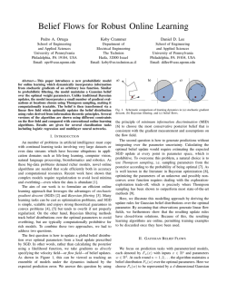


© Copyright 2026