1. Art and Diseño

The Bayes approach
Dipankar Bandyopadhyay
Div. of Biostatistics, School of Public Health, University of
Minnesota, Minneapolis, Minnesota, U.S.A.
1
Introduction
Start with a probability distribution f (y|θ ) for the data
y = (y1 , . . . , yn ) given a vector of unknown parameters
θ = (θ1 , . . . , θK ), and add a prior distribution p(θ |η ), where
η is a vector of hyperparameters
Inference for θ is based on its posterior distribution,
p(θ |y, η ) =
=
p(y, θ |η )
p(y, θ |η )
=
p(y, u|η ) du
p(y|η )
f (y|θ )p(θ |η )
f (y|θ )p(θ |η )
=
.
m(y|η )
f (y|u)p(u|η ) du
We refer to this formula as Bayes’ Theorem. Note its
similarity to the definition of conditional probability,
P(A|B) =
2
P(A ∩ B) P(B|A)P(A)
=
P(B)
P(B)
PuBH 7440: Introduction to Bayesian Inference
Example 2.2
Consider the normal (Gaussian) likelihood,
f (y|θ ) = N(y|θ , σ 2 ), y ∈ ℜ, θ ∈ ℜ, and σ > 0 known. Take
p(θ |η ) = N(θ |µ , τ 2 ), where µ ∈ ℜ and τ > 0 are known
hyperparameters, so that η = (µ , τ ). Then
p(θ |y) = N θ
Write B =
σ2
,
σ 2 +τ 2
σ 2 µ + τ 2y σ 2 τ 2
,
σ2 + τ2 σ2 + τ2
.
and note that 0 < B < 1. Then:
E(θ |y) = Bµ + (1 − B)y, a weighted average of the prior
mean and the observed data value, with weights
determined sensibly by the variances.
Var(θ |y) = Bτ 2 ≡ (1 − B)σ 2, smaller than τ 2 and σ 2 .
Precision (which is like "information") is additive:
Var−1(θ |y) = Var−1 (θ ) + Var−1(y|θ ).
3
PuBH 7440: Introduction to Bayesian Inference
Sufficiency still helps
Lemma: If S(y) is sufficient for θ , then p(θ |y) = p(θ |s), so
we may work with s instead of the entire dataset y.
Example 2.3: Consider again the normal/normal model
where we now have an independent sample of size n from
f (y|θ ). Since S(y) = y¯ is sufficient for θ , we have that
p(θ |y) = p(θ |¯y).
But since we know that f (¯y|θ ) = N(θ , σ 2 /n), previous slide
implies that
(σ 2 /n)µ + τ 2 y¯ (σ 2 /n)τ 2
,
(σ 2 /n) + τ 2 (σ 2 /n) + τ 2
σ 2 µ + nτ 2 y¯
σ 2τ 2
= N θ
,
.
σ 2 + nτ 2 σ 2 + nτ 2
p(θ |¯y) = N θ
4
PuBH 7440: Introduction to Bayesian Inference
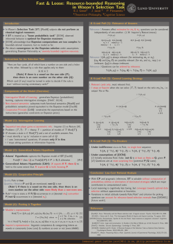
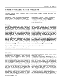
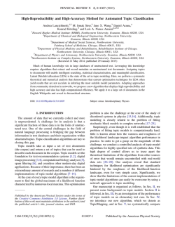
Example: µ = 2, y¯ = 6, τ = σ = 1
density
0.0
0.2
0.4
0.6
0.8
1.0
1.2
prior
posterior with n = 1
posterior with n = 10
-2
0
2
θ
4
6
8
When n = 1 the prior and likelihood receive equal weight,
so the posterior mean is 4 = 2+6
2 .
When n = 10 the data dominate the prior, resulting in a
posterior mean much closer to y¯ .
The posterior variance also shrinks as n gets larger; the
posterior collapses to a point mass on y¯ as n → ∞.
5
PuBH 7440: Introduction to Bayesian Inference
Three-stage Bayesian model
If we are unsure as to the proper value of the
hyperparameter η , the natural Bayesian solution would be
to quantify this uncertainty in a third-stage distribution,
sometimes called a hyperprior.
Denoting this distribution by h(η ), the desired posterior for
θ is now obtained by marginalizing over θ and η :
p(θ |y) =
=
6
p(y, θ , η ) dη
p(y, θ )
=
p(y)
p(y, u, η ) dη du
f (y|θ )p(θ |η )h(η ) dη
.
f (y|u)p(u|η )h(η ) dη du
PuBH 7440: Introduction to Bayesian Inference
Hierarchical modeling
The hyperprior for η might itself depend on a collection of
unknown parameters λ , resulting in a generalization of our
three-stage model to one having a third-stage prior h(η |λ )
and a fourth-stage hyperprior g(λ )...
This enterprise of specifying a model over several levels is
called hierarchical modeling, which is often helpful when
the data are nested:
Example: Test scores Yijk for student k in classroom j of
school i:
Yijk |θij ∼ N(θij , σ 2 )
θij |µi ∼ N(µi , τ 2 )
µi |λ ∼ N(λ , κ 2 )
Adding p(λ ) and possibly p(σ 2 , τ 2 , κ 2 ) completes the
specification!
7
PuBH 7440: Introduction to Bayesian Inference
Prediction
Returning to two-level models, we often write
p(θ |y) ∝ f (y|θ )p(θ ) ,
since the likelihood may be multiplied by any constant (or
any function of y alone) without altering p(θ |y).
If yn+1 is a future observation, independent of y given θ ,
then the predictive distribution for yn+1 is
p(yn+1 |y) =
f (yn+1 |θ )p(θ |y)dθ ,
thanks to the conditional independence of yn+1 and y.
The naive frequentist would use f (yn+1 |θ ) here, which is
correct only for large n (i.e., when p(θ |y) is a point mass at
θ ).
8
PuBH 7440: Introduction to Bayesian Inference
Prior Distributions
Suppose we require a prior distribution for
θ = true proportion of U.S. men who are HIV-positive.
We cannot appeal to the usual long-term frequency notion
of probability – it is not possible to even imagine “running
the HIV epidemic over again” and reobserving θ . Here θ is
random only because it is unknown to us.
Bayesian analysis is predicated on such a belief in
subjective probability and its quantification in a prior
distribution p(θ ). But:
How to create such a prior?
Are “objective” choices available?
9
PuBH 7440: Introduction to Bayesian Inference
Elicited Priors
Histogram approach: Assign probability masses to the
“possible” values in such a way that their sum is 1, and
their relative contributions reflect the experimenter’s prior
beliefs as closely as possible.
BUT: Awkward for continuous or unbounded θ .
Matching a functional form: Assume that the prior belongs
to a parametric distributional family p(θ |η ), choosing η so
that the result matches the elicitee’s true prior beliefs as
nearly as possible.
This approach limits the effort required of the elicitee, and
also overcomes the finite support problem inherent in the
histogram approach...
BUT: it may not be possible for the elicitee to “shoehorn” his
or her prior beliefs into any of the standard parametric
forms.
10
PuBH 7440: Introduction to Bayesian Inference
Conjugate Priors
Defined as one that leads to a posterior distribution
belonging to the same distributional family as the prior.
Example 2.7: Suppose that X is distributed Poisson(θ ), so
that
e−θ θ x
, x ∈ {0, 1, 2, . . .}, θ > 0.
f (x|θ ) =
x!
A reasonably flexible prior for θ having support on the
positive real line is the Gamma(α , β ) distribution,
p(θ ) =
11
θ α −1 e−θ /β
, θ > 0, α > 0, β > 0,
Γ(α )β α
PuBH 7440: Introduction to Bayesian Inference
Conjugate Priors
The posterior is then
p(θ |x) ∝ f (x|θ )p(θ )
∝
e−θ θ x
θ α −1 e−θ /β
= θ x+α −1 e−θ (1+1/β ) .
But this form is proportional to a Gamma(α ′ , β ′ ), where
α ′ = x + α and β ′ = (1 + 1/β )−1 .
Since this is the only function proportional to our form that
integrates to 1 and density functions uniquely determine
distributions, p(θ |x) must indeed be Gamma(α ′ , β ′ ), and the
gamma is the conjugate family for the Poisson likelihood.
12
PuBH 7440: Introduction to Bayesian Inference
Notes on conjugate priors
Can often guess the conjugate prior by looking at the
likelihood as a function of θ , instead of x.
In higher dimensions, priors that are conditionally
conjugate are often available (and helpful).
a finite mixture of conjugate priors may be sufficiently
flexible (allowing multimodality, heavier tails, etc.) while still
enabling simplified posterior calculations.
13
PuBH 7440: Introduction to Bayesian Inference
Noninformative Prior
– is one that does not favor one θ value over another
Examples:
Θ = {θ1 , . . . , θn } ⇒ p(θi ) = 1/n, i = 1, . . . , n
Θ = [a, b], −∞ < a < b < ∞
⇒ p(θ ) = 1/(b − a), a < θ < b
Θ = (−∞, ∞) ⇒ p(θ ) = c, any c > 0
This is an improper prior (does not integrate to 1), but its
use can still be legitimate if f (x|θ )dθ = K < ∞, since then
p(θ |x) =
f (x|θ ) · c
f (x|θ )
,
=
K
f (x|θ ) · c dθ
so the posterior is just the renormalized likelihood!
14
PuBH 7440: Introduction to Bayesian Inference
Jeffreys Prior
another noninformative prior, given in the univariate case
by
p(θ ) = [I(θ )]1/2 ,
where I(θ ) is the expected Fisher information in the model,
namely
∂2
log f (x|θ ) .
I(θ ) = −Ex|θ
∂θ2
Unlike the uniform, the Jeffreys prior is invariant to 1-1
transformations. That is, computing the Jeffreys prior for
some 1-1 transformation γ = g(θ ) directly produces the
same answer as computing the Jeffreys prior for θ and
subsequently performing the usual Jacobian
transformation to the γ scale (see p.99, problem 7).
15
PuBH 7440: Introduction to Bayesian Inference
Other Noninformative Priors
When f (x|θ ) = f (x − θ ) (location parameter family),
p(θ ) = 1, θ ∈ ℜ
is invariant under location transformations (Y = X + c).
When f (x|σ ) = σ1 f ( σx ), σ > 0 (scale parameter family),
p(σ ) =
1
, σ >0
σ
is invariant under scale transformations (Y = cX, c > 0).
When f (x|θ , σ ) = σ1 f ( x−σθ ) (location-scale family), prior
“independence” suggests
p(θ , σ ) =
16
1
, θ ∈ ℜ, σ > 0 .
σ
PuBH 7440: Introduction to Bayesian Inference
Bayesian Inference: Point Estimation
Easy! Simply choose an appropriate distributional
summary: posterior mean, median, or mode.
Mode is often easiest to compute (no integration), but is
often least representative of “middle”, especially for
one-tailed distributions.
Mean has the opposite property, tending to "chase" heavy
¯
tails (just like the sample mean X)
Median is probably the best compromise overall, though
can be awkward to compute, since it is the solution θ median
to
θ median
1
p(θ |x) dθ = .
2
−∞
17
PuBH 7440: Introduction to Bayesian Inference
Example: The General Linear Model
Let Y be an n × 1 data vector, X an n × p matrix of
covariates, and adopt the likelihood and prior structure,
Y|β ∼ Nn (X β , Σ) and β ∼ Np (Aα , V)
Then the posterior distribution of β |Y is
β |Y ∼ N (Dd, D) , where
D−1 = X T Σ−1 X + V −1 and d = X T Σ−1 Y + V −1Aα .
V −1 = 0 delivers a “flat” prior; if Σ = σ 2 Ip , we get
β |Y ∼ N βˆ , σ 2 (X ′ X)−1 , where
βˆ = (X ′ X)−1 X ′ y ⇐⇒ usual likelihood approach!
18
PuBH 7440: Introduction to Bayesian Inference
Bayesian Inference: Interval Estimation
The Bayesian analogue of a frequentist CI is referred to as
a credible set: a 100 × (1 − α )% credible set for θ is a
subset C of Θ such that
1 − α ≤ P(C|y) =
C
p(θ |y)dθ .
In continuous settings, we can obtain coverage exactly
1 − α at minimum size via the highest posterior density
(HPD) credible set,
C = {θ ∈ Θ : p(θ |y) ≥ k(α )} ,
where k(α ) is the largest constant such that
P(C|y) ≥ 1 − α .
19
PuBH 7440: Introduction to Bayesian Inference
Interval Estimation (cont’d)
Simpler alternative: the equal-tail set, which takes the α /2and (1 − α /2)-quantiles of p(θ |y).
Specifically, consider qL and qU , the α /2- and
(1 − α /2)-quantiles of p(θ |y):
qL
−∞
p(θ |y)dθ = α /2 and
∞
qU
p(θ |y)dθ = α /2 .
Then clearly P(qL < θ < qU |y) = 1 − α ; our confidence that
θ lies in (qL , qU ) is 100 × (1 − α )%. Thus this interval is a
100 × (1 − α )% credible set (“Bayesian CI”) for θ .
This interval is relatively easy to compute, and enjoys a
direct interpretation (“The probability that θ lies in (qL , qU )
is (1 − α )”) that the frequentist interval does not.
20
PuBH 7440: Introduction to Bayesian Inference
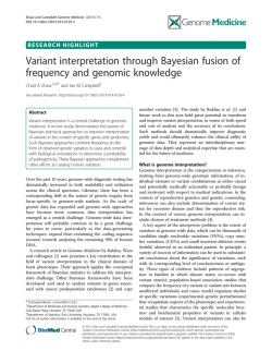
Interval Estimation: Example
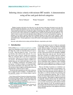
Using a Gamma(2, 1) posterior distribution and k(α ) = 0.1:
0.3
0.2
0.0
0.1
posterior density
0.4
87 % HPD interval, ( 0.12 , 3.59 )
87 % equal tail interval, ( 0.42 , 4.39 )
0
2
4
6
8
10
θ
Equal tail interval is a bit wider, but easier to compute (just two
gamma quantiles), and also transformation invariant.
21
PuBH 7440: Introduction to Bayesian Inference
1.5
0.0
0.5
1.0
posterior density
2.0
2.5
3.0
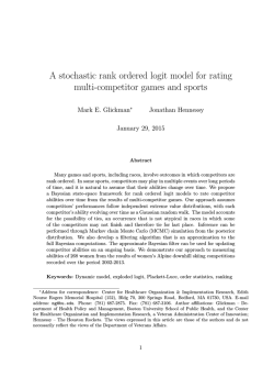
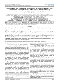
Ex: Y ∼ Bin(10, θ ), θ ∼ U(0, 1), yobs = 7
0.0
0.2
0.4
0.6
0.8
1.0
Plot Beta(yobs + 1, n − yobs + 1) = Beta(8, 4) posterior in R:
theta <- seq(from=0, to=1, length=101)
yobs <- 7; n <- 10;
plot(theta,dbeta(theta,yobs+1,n-yobs+1),type="l")
Add 95% equal-tail Bayesian CI (dotted vertical lines):
> abline(v=qbeta(.5, yobs+1, n-yobs+1))
> abline(v=qbeta(c(.025,.975),yobs+1,n-yobs+1),lty=2)
22
PuBH 7440: Introduction to Bayesian Inference
Bayesian hypothesis testing
Classical approach bases accept/reject decision on
p-value = P{T(Y) more “extreme” than T(yobs )|θ , H0 } ,
where “extremeness” is in the direction of HA
Several troubles with this approach:
hypotheses must be nested
p-value can only offer evidence against the null
p-value is not the “probability that H0 is true” (but is often
erroneously interpreted this way)
As a result of the dependence on “more extreme” T(Y)
values, two experiments with different designs but identical
likelihoods could result in different p-values, violating the
Likelihood Principle!
23
PuBH 7440: Introduction to Bayesian Inference
Bayesian hypothesis testing (cont’d)
Bayesian approach: Select the model with the largest
posterior probability, P(Mi |y) = p(y|Mi )p(Mi )/p(y),
where p(y|Mi ) =
f (y|θ i , Mi )πi (θ i )dθ i .
For two models, the quantity commonly used to summarize
these results is the Bayes factor,
BF =
P(M1 |y)/P(M2 |y) p(y | M1 )
=
,
P(M1 )/P(M2 )
p(y | M2 )
i.e., the likelihood ratio if both hypotheses are simple
Problem: If πi (θ i ) is improper, then p(y|Mi ) necessarily is
as well =⇒ BF is not well-defined!...
24
PuBH 7440: Introduction to Bayesian Inference
Bayesian hypothesis testing (cont’d)
When the BF is not well-defined, several alternatives:
Modify the definition of BF: partial Bayes factor, fractional
Bayes factor (text, p.54)
Switch to the conditional predictive distribution,
f (yi |y(i) ) =
f (y)
=
f (y(i) )
f (yi |θ , y(i) )p(θ |y(i) )dθ ,
which will be proper if p(θ |y(i) ) is. Assess model fit via plots
or a suitable summary (say, ∏ni=1 f (yi |y(i) )).
Penalized likelihood criteria: the Akaike information
criterion (AIC), Bayesian information criterion (BIC), or
Deviance information criterion (DIC).
IOU on all this – Chapter 4!
25
PuBH 7440: Introduction to Bayesian Inference
Example: Consumer preference data
Suppose 16 taste testers compare two types of ground
beef patty (one stored in a deep freeze, the other in a less
expensive freezer). The food chain is interested in whether
storage in the higher-quality freezer translates into a
"substantial improvement in taste."
Experiment: In a test kitchen, the patties are defrosted and
prepared by a single chef/statistician, who randomizes the
order in which the patties are served in double-blind
fashion.
Result: 13 of the 16 testers state a preference for the more
expensive patty.
26
PuBH 7440: Introduction to Bayesian Inference
Example: Consumer preference data
Likelihood: Let
θ
Yi
= prob. consumers prefer more expensive patty
1 if tester i prefers more expensive patty
=
0 otherwise
Assuming independent testers and constant θ , then if
X = ∑16
i=1 Yi , we have X|θ ∼ Binomial(16, θ ),
f (x|θ ) =
16 x
θ (1 − θ )16−x .
x
The beta distribution offers a conjugate family, since
p(θ ) =
27
Γ(α + β ) α −1
θ
(1 − θ )β −1 .
Γ(α )Γ(β )
PuBH 7440: Introduction to Bayesian Inference
Three ‘minimally informative’ priors
2.0
1.5
0.0
0.5
1.0
prior density
2.5
3.0
Beta(.5,.5) (Jeffreys prior)
Beta(1,1) (uniform prior)
Beta(2,2) (skeptical prior)
0.0
0.2
0.4
θ
0.6
0.8
1.0
The posterior is then Beta(x + α , 16 − x + β )...
28
PuBH 7440: Introduction to Bayesian Inference
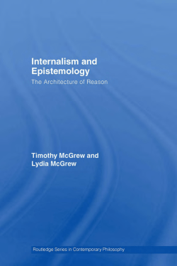
4
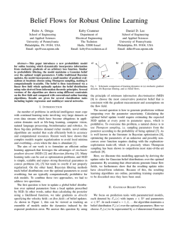
Three corresponding posteriors
2
0
1
posterior density
3
Beta(13.5,3.5)
Beta(14,4)
Beta(15,5)
0.0
0.2
0.4
0.6
0.8
1.0
θ
Note ordering of posteriors; consistent with priors.
All three produce 95% equal-tail credible intervals that exclude
0.5 ⇒ there is an improvement in taste.
29
PuBH 7440: Introduction to Bayesian Inference
Posterior summaries
Prior
distribution
Beta(.5, .5)
Beta(1, 1)
Beta(2, 2)
Posterior quantile
.025
.500
.975
0.579 0.806 0.944
0.566 0.788 0.932
0.544 0.758 0.909
P(θ > .6|x)
0.964
0.954
0.930
Suppose we define ‘substantial improvement in taste’ as
θ ≥ 0.6. Then under the uniform prior, the Bayes factor in
favor of M1 : θ ≥ 0.6 over M2 : θ < 0.6 is
BF =
0.954/0.046
= 31.1 ,
0.4/0.6
or fairly strong evidence (adjusted odds about 30:1) in
favor of a substantial improvement in taste.
30
PuBH 7440: Introduction to Bayesian Inference