1. Art and Diseño

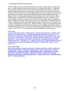
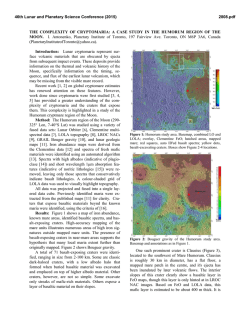
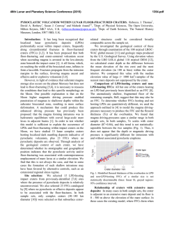
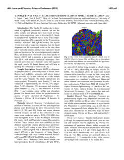
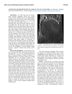
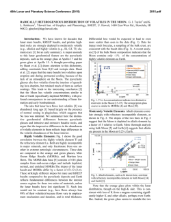
46th Lunar and Planetary Science Conference (2015)
2691.pdf
CONSTRAINTS ON THE DISTRIBUTION AND THICKNESS OF MARE BASALTS AND
CRYPTOMARE FROM GRAIL. Shengxia Gong1,2, Mark A. Wieczorek2, Francis Nimmo3, Walter S. Kiefer4,
James W. Head5, David E. Smith6, Maria T. Zuber6. 1Shanghai Astronomical Observatory, Chinese Academy of
Sciences, 200030 Shanghai, China ([email protected]), 2Insitut de Physique du Globe de Paris, Sorbonne Paris
Cité, Université Paris Diderot, 75013 Paris, France, 3Department of Earth and Planetary Sciences, University of California Santa Cruz, Santa Cruz, CA 95064, USA, 4Lunar and Planetary Institute, Houston, TX 77058, USA,
5
Department of Earth, Environmental and Planetary Sciences, Brown University, Providence, RI 02912, USA.
6
Department of Earth, Atmospheric, and Planetary Sciences, Massachusetts Institute of Technology, Cambridge,
MA 02139, USA
Introduction. Mare basalts are derived from partial melting of the lunar interior, with most being located on the near side of the Moon [1, 2]. The total
volume and spatial distribution of these basalts provide
crucial information about both the Moon’s thermal
evolution and volcanic activity. Unfortunately, the
thicknesses of the mare are only poorly constrained,
and in some cases, old basalts are hidden from view,
being covered by ejecta from large craters.
We use gravity data from NASA’s Gravity Recovery and Interior Laboratory (GRAIL) mission to investigate the mare basalts. Using an approach pioneered
by Besserer et al. [3], we search for buried lava deposits, also known as cryptomaria [4,5], and invert for the
thicknesses of the major mare basalt flows.
Distribution of mare basalts. Mare basalts, which
have lower albedo and higher density than the highlands crust, have been mapped using orbital and telescopic images (Fig. 1). However, it has long been suspected that some portion of these basalts, in particular
the most ancient units, might have been buried by the
ejecta from adjacent impact basins and craters.
Besserer et al. developed a method for constraining
the depth dependence of density below the surface by
use of an “effective density” spectrum [3], which is
simply the ratio of the free-air gravity and the gravity
predicted from unit-density topography as a function of
spherical harmonic degree. The short wavelengths of
this function are most sensitive to the surface density,
whereas longer wavelengths sample deeper depths.
Localized estimates of the effective density spectrum,
obtained from a multitaper spectral analysis, are then
compared to an analytical model that depends on the
subsurface density profile.
We expand upon the work of Besserer et al. [3] by
considering the most recent GRAIL gravity models
and by using smaller, higher spatial-resolution windows in the multitaper spectral analysis [6]. We find
that spherical cap windows with an angular radius of
10° in radius, and a fewer number of tapers (N=5),
provide adequate resolution to investigate the density
profile. Besserer et al. used; in contrast, windows with
an angular radius of 15°.
Our analyses were centered on 400 grid nodes as
shown in Fig 2. In this preliminary analysis, only the
spherical harmonic degree range from 250 to 550 was
considered.
Using a theoretical model with a linear dependence
of density with depth, we invert for the density gradient. Besserer et al. [3] showed that this gradient was
generally negative in the mare, where dense basalts
overlay less dense highland materials. In contrast, they
found that density increases with depth in the highlands, most likely due to the compaction of porosity.
We use negative density gradients as a proxy for the
presence of mare and cryptomare basalts.
90˚
60˚
30˚
0˚
−30˚
−60˚
−90˚
−180˚ −150˚ −120˚ −90˚
−60˚
−30˚
0˚
30˚
60˚
90˚
−30˚
0˚
30˚
60˚
90˚
120˚
150˚
180˚
150˚
180˚
90˚
60˚
30˚
0˚
−30˚
−60˚
−90˚
−180˚ −150˚ −120˚ −90˚
−40
−30
−60˚
−20
−10
0
10
20
120˚
30
40
Density gradient (kg m−1 km−1)
Figure 1. (top) Distribution of mare basalts as mapped by
the USGS. The locations of identified cryptomare Taruntius
and Cleomedes are shown as triangles, possible GRAIL identified cryptomare are shown as squares, and the cryptomare
Schiller-Schickard is marked by a star. (bottom) Subsurface
density gradient from GRAIL gravity, with negative gradients in blue and positive gradients in red. White dots mark
the locations of the 400 grid nodes used in this work.
46th Lunar and Planetary Science Conference (2015)
Conclusion: GRAIL gravity is sensitive to both the
distribution and thickness of mare basalts. Preliminary
investigations have shown that it should be possible to
detect cryptomaria using estimates of the density gradient in the upper crust. Future work in this direction
will involve detailed comparisons of our density gradient maps with maps of mare basalts and proposed
cryptomaria [7]. Furthermore, it should be possible to
invert for the thickness of the mare basalts by use of
the effective density spectrum. The validity of this
technique will be assessed by comparison to independent estimates obtained from radar sounding data and
estimates based on the composition of crater ejecta.
2600
2500
Effective density
In Fig. 1, we plot our inverted subsurface density
gradient as a function of location on the surface. Most
of the known mare basalts are found to have negative
gradients. Nevertheless, some regions of known basalts
turn out to have positive gradients, such as in northern
Oceanus Procellarum. Several possibilities exist for
this apparent discrepancy, such as a more mafic underlying crust, important stratification in basalt density,
and perhaps .an insensitivity to the basalts if they are
extremely thin.
Negative density gradients are sometimes found in
the highlands, and we propose that these regions might
represent areas where dense mare basalts were overlain
by a thin surficial layer of higher-albedo highlands
ejecta. Prominent regions of interest that have previously been recognized as cryptomare include a region
west of Taruntius (5.01° N, 45.23° E) and Cleomedes
(27.55° N, 55.93° E) [7]. Regions that have not previously been identified as cryptomare include a region
north of Mare Imbrium (80° N, 30° W) and a region
west of Mare Nectaris. The well-known SchillerSchickard cryptomare (48.92° S, 51.75° W) does not
appear to be associated with a negative gradient in our
analysis.
Thickness of mare basalts. The total volume of
mare basalts is an important quantity for deciphering
the Moon’s thermal evolution [2]. We propose to use
GRAIL-derived localized effective density spectra to
invert for the thickness of the mare. A simple theoretical model was constructed in spherical harmonics under the assumption that a constant thickness layer of
dense mare basalts overlies a less dense crust. This
model depends upon the assumed layer densities, as
well as the thickness of the basalts.
Using measured grain densities (3270–3460 kg/m3)
and porosities (2-7%) of the mare basalts [8], we set
the density of the upper basalt layer to 3010-3270
kg/m3. For the bulk density of lower layer, we use a
typical highland value of 2590-2870 kg/m3 [9].
Fig. 2 shows the theoretical effective density spectra for different basalts thickness: 100 meters, 1 km,
and 5 km. These curves clearly show that the effective
density spectrum is sensitive to basalt thickness, which
should allow us, in principle, to constrain this value.
Also shown is one representative effective density
spectrum obtained from the nearside mare for comparison.
In our ongoing work, we will use the observed effective density spectrum, along with a priori constraints on basalt density from composition [10], to
constrain the mare thickness. These values will be
compared to independent thickness estimates made
from radar sounding data [11], impact ejecta studies
[e.g., 12], and basin depth-diameter relationships [13].
2691.pdf
2400
2300
2200
2100
2000
200
300
400
500
600
700
Spherical harmonic degree
Figure 2. Effective density spectrum for a representative
region in the nearside mare (0o,40oE). The black line is the
observed effective density spectrum, with gray lines representing ±1 standard errors. The blue, green, and red lines
represent the theoretical effective density spectrum for basalt
thickness of 100 m, 3 km, and 5 km, respectively.
References:
[1] Wieczorek M. A. and Phillips R. J. (2000), J.
Geophys. Res. 105(E8), 20417-20430. [2] Head J. W.
(1976), Rev. Geophys. Space Phys., 14, 265-300. [3]
Besserer J. et al. (2014), Geophys. Res. Lett., 41, 5771–
5777. [4] Head J .W. and Wilson L. (1992), Geochim.
Cosmochim. Acta., 56, 2155-2175. [5] Sori et al.
(2013), Lunar Planet. Sci. Conf., 44th, abstract 2755.
[6] Wieczorek M. A. and Simons F. J. (2007), J. Fourier Anal. Appl., 13(6), 665-692. [7] Whitten J. L. and
Head J. W. (2015) Icarus, 247, 150-171. [8] Kiefer W.
S. et al. (2012) Geophys. Res. Lett., 39, L07201. [9]
Wieczorek M. A. et al. (2013), Science, 339, 671-675.
[10] Huang Q. and Wieczorek M. A. (2012), J. Geophys. Res., 117, E05003. [11] Peeples, W. J., et al.
(1978) J. Geophys. Res., 83, 3459–3468. [12] Budney
C. J and P. G. Lucey (1998), J. Geophys. Res., 103,
16,855-16,870. [13] Dibb S. D. and Kiefer W. S., Lunar Planet. Sci. Conf. 46th, abstract 1677, this conference.