1. Art and Diseño

Bulletin of the Seismological Society of America, Vol. 74, No. 5, pp. 1969-1993, October 1984
A MODEL FOR THE SHAPE OF THE FOURIER AMPLITUDE
SPECTRUM OF ACCELERATION AT HIGH FREQUENCIES
BY JOHN G. ANDERSON AND SUSAN E. HOUGH
ABSTRACT
At high frequencies f the spectrum of S-wave accelerations is characterized
by a trend of exponential decay, e -~". In our study, the spectral decay parameter
shows little variation at a single station for multiple earthquakes at the same
distances, but it increases gradually as the epicentral distance increases. For
multiple recordings of the San Femando earthquake, x increases slowly with
distance, and x is systematically smaller for sites on rock than for sites on
alluvium. Under the assumption that the Fourier spectrum of acceleration at the
source is constant above the comer frequency (an , - 2 source model), the
exponential decay is consistent with an attenuation model in which Q increases
rapidly with depth in the shallow crustal layers.
INTRODUCTION
The shape and amplitude of the Fourier amplitude spectrum of strong ground
acceleration is recognized as useful for various applications to earthquake engineering (McGuire, 1978). This acceleration spectrum also contains fundamental information about physical processes at the earthquake source and wave propagation in
the crust of the earth. Yet at high frequencies, we still do not have a satisfactory
model for the shape of the acceleration spectrum. By the shape of a spectrum we
refer to a smooth trend through the spectrum; the fine structure which is superimposed on this trend is not meant to be included.
At low frequencies and sufficiently far from the fault, the inevitable result of an
elastic rebound source model is that the acceleration spectrum increases as w2,
where ~ = 2~[ and [ is the frequency of ground motion. For example, a widely
employed model by Brune (1970) relates the coefficient of this w2 trend to the
seismic moment, Mo, and relates the corner frequency ([0) where this w2 trend
terminates to a stress drop parameter at the source. Above the corner frequency,
Trifunac (1976) and McGuire (1978) have carried out empirical regressions for the
shape of the acceleration spectrum but these regressions do not yield much insight
into the physical processes which are involved. Hanks (1979, 1982) suggests that,
in general, the acceleration spectrum is fiat above the corner frequency to a second
corner frequency (/max) above which the spectrum decays rapidly.
In the next section, we propose a parametric shape for the acceleration spectrum
at high frequency. Our model is characterized by one parameter, which we designate
as the spectral decay parameter K. Recognition and study of this parameter were
motivated in part by the observations that most spectra observed in the 1981 Santa
Barbara Island earthquake appear to fall off exponentially (Anderson, 1984). Subsequent sections explore the systematic behavior of Kfor the S-wave portion of the
accelerogram. We also recognize a plausible attenuation model to explain the
observations but intentionally avoid introducing the terminology and notation of
that model into the observation sections of this paper.
SPECTRAL SHAPE AT HIGH FREQUENCIES
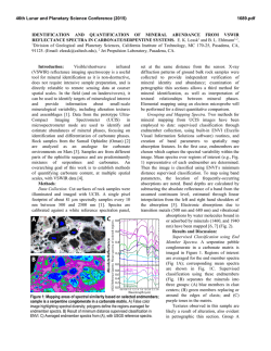
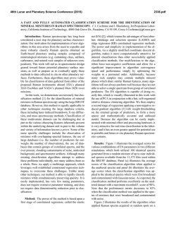
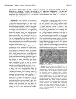
Figure 1 shows the Fourier amplitude spectrum of acceleration for the $16°E
component of the Pacoima Dam accelerogram from the 1971 San Fernando, Cali1969
1970
JOHN G. ANDERSON AND SUSAN E. HOUGH
fornia, earthquake. Figure 1A shows the spectrum plotted on log-log axes. Based on
a figure of this type, Hanks (1982, Figure 2) selects/max for this record to be near
10 Hz. In Figure 1B, the frequency axis is linear. On these axes, the dominant trend
is a linear decrease of the log of spectral amplitude with frequency, and there is no
apparent additional slope break in the vicinity of 10 Hz. In some cases, the dominant
trend of exponential decay is initiated near/o, but on other spectra it begins at
some higher frequency. It is, therefore, useful to label the frequency above which
the spectral shape is indistinguishable from exponential decay. Here we call this
frequency rE. We do not ascribe any fundamental importance to rE, and pay little
attention to it in the rest of this paper. Considering the amplitude of the fine
PACOIMA DAM ($16E COMP)
104
~
103
n~
I-0
m
n
(,0
h
0
(b
0
102
101
100
10-1
I
I
IIIIIII
0-2
I
x
[
IlJllll
10 -1
I
I
I]1111[
10 0
I
I
101
llllJ
10 2
LOG OF FREQUENCY
10 4
~E
10 3
t~
0
m
0_
10 2
h
0
101
(.~
q
10 0
10-1
-5
I
I
0
5
L
I
I
10
15
20
FREQUENCY
I
25
30
Fro. 1. Fourieramplitude spectrum of acceleration for the $16°E component of the Pacoima Dam
accelerogram, San Fernando, California,earthquake of 9 February 1971. Accelerogramwas digitzedby
hand. (A) Log-logaxes. (B) Linear-logaxes.
structure to the spectrum (Figure 1), it is difficult to determine meaningful trends
over narrow frequency bands (e.g., bandwidth less than about 3 to 5 Hz). Thus the
identification of rE, like that of [max, is to some extent subjective. On Figure 1,/E
may occur between 2 and 5 Hz. Thus, on this spectrum, fE is distinctly less than
the value for [maxwhich was identified by Hanks (1982).
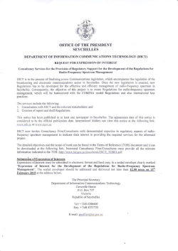
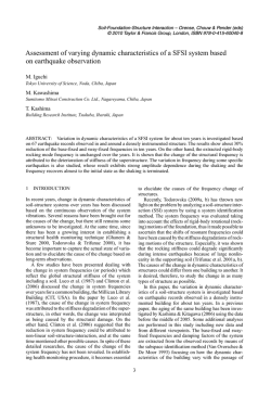
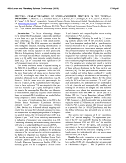
Figure 2 is the equivalent of Figure 1, but for the spectrum of an accelerogram
recorded at Cucapah, Baja California, Mexico, from the June 1980 earthquake (ML
= 6.1) in the Mexicali Valley, across the international border from the Imperial
Valley, California. These data are described by Anderson et al. (1982). The accelerograph in this case is a digital recorder (Kinemetrics DSA-1) which samples the
output of a force-balance accelerometer (natural frequency 50 Hz) at a rate of 200
samples/sec, so that the Nyquist frequency is 100 Hz. The least count is about 0.5
A MODEL FOR ACCELERATION SPECTRUM AT HIGH FREQUENCIES
1971
cm/sec 2. Because the response of the force-balance sensor is flat to 50 Hz, no
instrument correction has been applied to this record. Because of the highly accurate
digital recording, there is little uncertainty about the reliability of the digitization
on this record, as there might be for hand-digitized data {e.g., Berrill and Hanks,
1974; Sacks, 1980; Cormier, 1982).
Figure 2A shows the same general properties as Figure 1A, although the window
in this case was not long enough to establish a low-frequency asymptote at frequencies less than the corner frequency )Co.By analogy to Figure 1A, one would pick [max
at about 10 Hz for the spectrum in Figure 2A. Figure 2B again shows a predominantly
exponential decrease in spectral amplitude, in this case from 1 to 40 Hz. Below
CUCAPAH
June 9 , 1 9 8 0
85 °
03 .'28 GMT
102
A
frnox
101
10°
ILl
03
10-1
hi
,m
10-2
10-2
t--
10-I
100
101
LOG OF FREQUENCY
._1
<
I-(.3
Ld
13_
03
102
102
B
101
10o
0
20
40
60
FREQUENCY (Hz)
80
100
FIO. 2. Fourier amplitude spectrum of the N85°E component of strong ground acceleration recorded
at Cucapah during the Mexicali Valley earthquake of 9 June 1980 (ML = 6.2). Accelerograph was a digital
recorder which samples at a rate of 200/sec. (A) Log-log axes. (B) Linear-log axes.
about 6 Hz, there is again room to define, at a lower confidence level, a trend which
diverges from the exponential trend which dominates over the full frequency band.
At 40 Hz the exponential trend intersects spectral amplitudes of about 0.1 cm/sec,
corresponding to the least count digitization level, and above 40 Hz the spectrum is
flat, as is appropriate for a digitization process with random round-off errors at an
amplitude of +0.5 least count.
Based on Figures 1 and 2, and many comparable spectral plots, we hypothesize
that to first order the shape of the acceleration spectrum at high frequencies can
generally be described by the equation
a ( f ) = Aoe -'~/
f > fE
(1)
1972
JOHN G. ANDERSON AND SUSAN E. HOUGH
where Ao depends on source properties, epicentral distance, and perhaps other
factors. The systematic behavior of the spectral decay parameter K is explored in
the next three sections of this paper.
METHOD
We studied shear-wave spectra for the horizontal components of strong ground
acceleration from 98 sites around the 1971 San Fernando earthquake, ten events
recorded at Ferndale, ten events recorded at El Centro, and five events recorded at
Hollister. All records are corrected accelerograms from the Volume II data tape
prepared by the Earthquake Engineering Research Laborartory of California Institute of Technology (EERL, 1971).
Fourier transforms of the shear waves were computed from accelerograms. The
time window was chosen to include only direct S-wave arrivals. In cases where the
transition from direct S-wave arrivals to coda was not readily apparent, our choice
for the time window favored including coda rather than possibly eliminating direct
arrivals. Spectral shape was found to be fairly insensitive to the time window length
as long as it was reasonably chosen. The value of K at stations ~40 km from the
epicenter of the San Fernando earthquake showed no correlations with time window
length. The transforms were computed with a standard Fast Fourier transform
routine after a cosine taper was applied to the raw data and the time series were
padded out to powers of two with zeroes. The spectra were plotted from 0 to 25 Hz
(Nyquist frequency = 25 Hz).
To obtain the spectral decay parameter, linear least-squares fits to the spectra
were obtained. A 2- to 12-Hz interval was used for the El Centro, Ferndale, and
Hollister records. The corner frequencies for all of the earthquakes we considered
are less than 2 Hz. Frequencies higher than 12 Hz were considered potentially
unreliable on some of these records in these data sets for reasons to be discussed
later. For the San Fernando records, the interval used for regression was 2 to 18
Hz.
Values of the slopes were converted to the spectral decay parameter, K, and
subsequently plotted against epicentral distance to evaluate distance-dependence.
To quantify trends, we found a linear regression between K and distance, R, even
though we do not believe a linear relationship is the definitive dependence of K on
R. For the multiple event data, these straight lines were fit directly. The San
Fernando data were averaged within 10-km distance bands and then fit with straight
lines. This latter procedure reduces the weight of the distance ranges which are
represented by large numbers of stations. Regression done on the complete data
sets yielded similar results.
RESULTS: SINGLE STATION AND MULTIPLE EVENTS
Figures 3 through 9 illustrate results for records of earthquakes at multiple
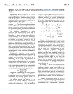
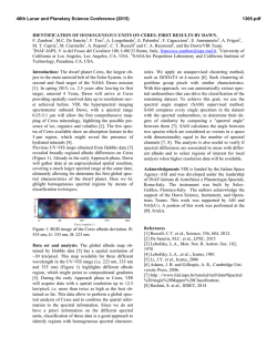
distances from a single station. Figure 3 is a map of the vicinity of the E1 Centro
accelerograph, showing locations of the station, epicenters of ten earthquakes which
were recorded on the accelerograph, and generalized surficial geology. Corresponding
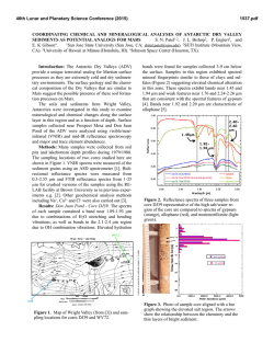
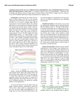
S-wave spectra and least-squares fits are shown in Figure 4. Figure 5 is a map of
the Ferndale vicinity, and Figure 6 shows corresponding spectra for ten earthquakes
which have been recorded there. Locations of the earlier earthquakes recorded at
El Centro and Ferndale may have substantial errors. The 1934 and 1954 earthquakes
at E1 Centro are shown at the relocated epicenters of Leeds (1979). These epicenters
may be more reliable than others among the earlier earthquakes on these maps.
1973
A MODEL FOR ACCELERATION SPECTRUM AT HIGH FREQUENCIES
Figure 7 is a map of the Hollister vicinity and Figure 8 shows corresponding spectra
for five earthquakes recorded at Hollister. Finally, Table 1 and Figure 9 show
measured values of Kas a function of distance for all three stations.
Figure 4 shows spectra for both components of the El Centro station. On these
spectra, a linear trend dominates the spectral shapes for frequencies between 2 and
ft6 o
I
i~, .:
f f5 o
1t5°30 '
~+~i~i~i~i~:!+i
%iiiiiii!i!!i!~~::¸.
i ~::~:~:~i~!ii !!ii i i i i i i !i i i i i i~....
+~i
ff4°30
I
I
33030 ,
33o30
I ]
'
Quafernoc, Alluvium
Te¢tiory Sedimentary
Rocks
So/ton sea
•195t
33 °
::i;ii:i; !ii:iiii~!:!i~:
1942 (6.5)::
Crylfolline ROCks
f955
T292
.~ +.J
(5.6)
T287
!J, f953
0
(5.4
L
I
I
33 °
(5.5)
El Centro ~1:,
Station
~ ",
~1940 (6.7)
"~
, ,. " "
AOOt
~
united s t a t e s _
•~
-
Mexico
+
\
32o30 '
32030 '
1934
(6.5)
B024
32 °
32 °
f966
(63)
T293
116 o
f15o30 '
ff5 °
114+30 '
FIG. 3. Map of Imperial Valley, California-Mexico showing generalized geological features. Epicenters
(asterisk) from Leeds (1979) or Hileman et al. (1973) are shown with year and magnitudes of earthquakes
which have generated accelerograms at the E1 Centro station. Accelerogram number on the Caltech tapes
is given below year. The 1940 and 1968 ruptures are from Jennings {1975).
12 Hz. Spectra for the 1934, 1940, and 1942 earthquakes (records B024, A001, and
T286, respectively) have a nearly level trend starting at frequencies between 12 and
15 Hz. Likewise in Figure 6 many of the spectra, and most conspicuously the spectra
for the earliest earthquakes, appear to assume a nearly level trend starting at
JOHN G. ANDERSON AND SUSAN E. HOUGH
1974
frequencies as low as about 12 Hz. In Figure 8 all of the spectra deviate above the
linear trend starting at between 12 and 15 Hz. In Figure 2, similar behavior resulted
from the digitization, thus suggesting that digitization has also caused level spectral
trends on these accelerograms.
An estimate for the typical range for the Fourier amplitude of digitization noise
for these hand-digitized accelerograms has been presented by Berrill and Hanks
(1974). Noise amplitudes under the digitization conditions of these accelerograms
EL
270
CENTRO
°
180 °
±
1 unit
T
T
,'
M
l' '
-
~b.,..
72.,20,+
T289
(.)
.... ,...
+++
E
127 km
v
~
E
~
Z3
(./3
cO
~
~
~
<
/0
~
_
10 z
101
100
10-1
0
,,
I~"--.~.~h.~hlhL/
'
727
km
AOt9
70 km
B024
61 km
" ,
T
286
46 km
~
T286
~
7287
27 km
T287
27 km
I p
|
~
l
~
7288
24 km
T288
24 km
T292
23 km
AO01
9 km
T292
km
23
9krn
AOOi
I
I
I
L
i
I
5
10
15
20
25
50
0
I
5
I
10
I
t5
I
20
I
25
Frequency ( H z )
FIG. 4. Fourier amplitude spectra of S-wave accelerograms corresponding to epicenters from Figure
3. Record number and distance from the accelerograph are indicated to right of each spectrum. Each
spectrum is offset by two logarithmic units from the spectrum immediately below. Superimposed on each
spectrum is a linear, least-squares fit over the frequency band 2 to 12 Hz.
and the signal window employed in our study decrease smoothly from about 0.3 +
0.07 cm/sec at 1 Hz to 0.18 _ 0.06 cm/sec at 12 Hz, and 0.11 _ 0.03 cm/sec at 24
Hz. Deviations of S-wave spectra above an exponential decay approximately coincide with these levels for all Hollister spectra (Figure 8) and for E1 Centro and
Ferndale spectra of earthquakes recorded after 1949 (Figures 4 and 6).
All of the pre-1948 spectra from E1 Centro and Ferndale form a trend parallel to
the digitization noise but the amplitude of this trend exceeds the amplitudes found
I
50
A MODEL FOR ACCELERATION SPECTRUM AT HIGH FREQUENCIES
1975
by Berrill and Hanks {1974). It turns out that instrumental characteristics of the
acclerographs at E1 Centro and Ferndale were modified once. Before the modification, the undamped natural frequency of each sensor was about 10 Hz (e.g., Bodel,
1944). Beginning in 1942, the U.S. Coast and Geodetic Survey began to modify its
accelerographs to reduce the gain at selected stations. This modification was made
at E1 Centro and at Ferndale in late 1948 or early 1949, based on a review of
instrument constants published in the series United States Earthquakes (see Murf25 °
f24 °
f23*W
4f °
4f o
"~ f9
8C
40°N
40°N
f25"
t24 °
f23*W
FIG. 5. Map of Cape Mendocino, California, showing generalized geological features. Epicenters from
Trifunac and Lee (1978) are identified with the same notations as in Figure 3 and represent earthquakes
which have produced accelerograms on the Ferndale accelerograph. The 1934, M = 6.0 earthquake
(Record U294) was located off map at 41.7°N, 124.6°W. Real et al. (1978) location for the 1938 earthquake
is 40°N, 124°W, about 75 km from the epicenter shown here.
phy and Ulrich, 1951a, b). Subsequently, the natural frequencies of the sensors were
between 15 and 16 Hz. Thus, if we assume that the digitization and instrument
correction procedure for the pre-1948 earthquakes leads to digitization noise above
the level described by Berrill and Hanks (1974), the deviations of spectra in Figures
4, 6, and 8 above the model of exponential decay are all explained by digitization
noise.
For the 1953 event, the north-south component at E1 Centro may have been
working improperly based on the appearance of the original accelerogram in Murphy
and Cloud (1955) and spectral levels nearly an order of magnitude less than for the
east-west component. The same trace was defective for the record of the 21 July
1952 Kern County earthquake (Murphy and Cloud, 1954). We have thus not
included that measurement of K on Figure 9, even though it is consistent with other
values.
The E1 Centro station data in Figure 4 show that the spectral slopes of the two
1976
J O H N G. ANDERSON AND SUSAN E. HOUGH
horizontal components of S waves from an earthquake are similar. Spectra in Figure
4, generally arranged from farthest to nearest, show a weak but clear distance
dependence of the spectral shape, which is confirmed in Table 1 by the numerical
values of the spectral decay parameters. The least-squares line through these data
on Figure 9 has the equation K = 0.054 sec 4- {0.00041 sec/km)R, where R is the
source-to-station distance.
Accelerograms which have been recorded at Ferndale are primarily from offshore
locations (Figure 5), and many of the epicenters are not well controlled. Spectra
(Figure 6) show a less conspicuous increase of K with distance than for El Centro
FERNDALE
±
I unil
T
I•IL.
L .b.
•
o
~)ql"'F~~,,=,.,.
E
"
•
[T ~
• --
., U 2 9 4
1 2 9 km
I ~ I ~ t l ~ I~,~,~1~~.,~ u 2 9 8
,
! '
~
"
"lMdL.l.,,
"5o_o
~...~~~l~i~Ji " ~
O0
~rni.~,i,:',~',B~,~,~t~.,,.,
E
._o
"~
B027
. . . .
U308
"Viff'~ 60 kn~
,
.
AO02
I I p" l'ifill'll,Wllr1~rdl~ s o z 6
'
" r
' pl'155k
m
-
¢J
B030
_-I
r ~
I
~
1
~
1
~
~
AO09
4.o,r.
i
10 0
--'<'~E"~
I
rl~'l~lhk,~.hJ.
-
r~rr,
,..A~._.,,~,,
31 kr.
~,,U300
,..,
,
o
5
Io
t5
20
25
30
Frequency (Hz)
FIG. 6. S-wave acceleration spectra from Ferndale site for earthquakes on Figure 5. Please refer to
Figure 4 caption for other notation.
records. The least-squares fit to the Ferndale data on Figure 9 is K = 0.075 sec +
(0.00016 sec/km)R. Spectra from Hollister {Figure 8) do not show a conclusive
change in the spectral decay parameter with distance, but all the accelerograms
were obtained at distances of less than 40 km.
Figure 9 summarizes the three studies of multiple recordings at a single station.
At E1 Centro, Ferndale, and Hollister, the spectral decay parameter exhibits a
common type of behavior. Within the resolution of the data, Ktends toward a finite
value as epicentral distance approaches zero; we interpret this finite value as a
characteristic of the subsurface geological structures. The term "subsurface geological structure" is used in the sense employed by Dobrin (1960) to refer to geological
conditions below and near the site within distances on the order of hundreds of
A MODEL
F O R A C C E L E R A T I O N S P E C T R U M AT H I G H F R E Q U E N C I E S
1977
meters to a few kilometers. In addition to the subsurface geology effect, a pathdistance effect also seems to be present and causes K to increase gradually with
distance. The existence of this systematic behavior suggests that the source spectral
shapes of the several earthquakes probably had identical trends between the
frequencies of 2 and 12 Hz.
TABLE 1
SPECTRAL DECAY PARAMETERS FOR ACCELEROGRAMS RECORDED
AT HOLLISTER, FERNDALE, AND EL CENTRO
Record
Distance Magnitude
K1
Date
K2
HOLLISTER
03/09/49
04/25/54
01/19/60
04/08/61
12/18/67
U301
U305
U307
U309
U313
19.9
29.1
8.5
19.8
39.0
10/07/51
12/21/54
09/11/38
02/09/41
09/22/52
07/06/34
02/06/37
10/03/41
06/05/60
12/10/67
A002
A009
B026
B027
B030
U294
U298
U300
U308
U312
56.3
40.4
55.3
98.4
45.2
128.9
85.1
29.8
60.3
30.6
05/19/40
02/09/56
04/08/68
12/30/34
10/21/42
01/23/51
06/13/53
11/12/54
12/16/55
08/07/66
A001
A011
A019
B024
T286
T287
T288
T289
T292
T293
5.3
5.3
5.0
5.6
5.8
0.0850
0.0828
0.0865
0.0667
0.0880
FERNDALE
5.8
6.5
5.5
6.4
5.5
6.0
5.8
6.4
5.7
5.6
0.0858
0.0821
0.0909
0.0909
0.0887
0.0923
0.1019
0.1114
0.0667
0.0447
EL CENTRO
RESULTS:
9.3
126.9
69.8
60.8
46.5
27.5
23.6
119.8
23.5
148.1
6.7
6.8
6.4
6.5
6.5
5.6
5.5
6.3
5.4
6.3
0.0608
0.0945
0.1011
0.0682
0.0645
0.0770
0.0591
0.0923
0.0452
0.1048
0.0806
0.1077
0.0938
0.0711
0.0645
0.0630
0.0751
0.0975
0.0369
0.1217
SAN FERNANDO EARTHQUAKE
The San Fernando earthquake represents a situationin which multiple recordings
have been made of a single event. Azimuthal variations in K resulting from the
source function were assumed negligibleeven though radiation at frequencies of 4
Hz and lower might be affectedby source directivity(Berrill,1975). This earthquake
was used to study the effect of variable local geology and distance on K. A map
showing station locations and generalized geology has been prepared by Hanks
(1975).
About 90 per cent of the spectra from the San Fernando records have an average
trend which is modeled well by equation (1). The other 10 per cent of the records
often appear to follow the same trend, except for a superimposed bulge which we
1978
JOHN
G. A N D E R S O N A N D S U S A N E. H O U G H
tentatively identify as a site amplification effect. Figure 10 shows one of the more
conspicuous examples of Fourier spectra with a relatively large apparent amplification of this type. Smaller broadband resonances may be unrecognized, and we
conjecture that such resonances may add noise to determinations of K.
Table 2 and Figure 11 summarize values of K obtained from the San Fernando
earthquake. Table 2 also lists the distance, the window length employed (T), and
site classification, S. In Figure 11, the stations were grouped into three categories:
alluvium (S = 0), consolidated sedimentary rock (S = 1), and hard (igneous or
metamorphic) rock (S = 2), following the site classification of Trifunac and Brady
(1975). Stations listed as being on sedimentary rocks actually include sites on
f22 °
•
f21 °
%
o
50
(5.3:
37 °
3T o
Pacific
Ocean
"
~gsr (5.8)
",.~:~
1954 (5.3)
\
~,
U305
~
Mo.teray
\
~
\
t
(50
U307 ~i::ii~~
1960
SoX
\
t961 (5.6)
\
7'
,
I--]
\
Quaternary Alluvium
~
•
\
Tertiary
Sedimentary %
Rocks
\
Mesozoic Sedimentary
Rocks
'\
~.
",,,
.,,,
Crystalline Rocks
36 °
36 o
122"
12P
FIG. 7. M a p of central California showing generalized geological features. Epicenters from Real e t a l .
(1978) are identified with t h e s a m e n o t a t i o n as in Figure 3 a n d represent e a r t h q u a k e s which have
produced accelerograms on t h e Hollister accelerograph.
shallow alluvium as well as those on consolidated sediments. In this manner, the
site classifications of Trifunac and Brady (1975) attempt to account for subsurface
geological structure as well as conditions in the immediate vicinity of the site.
Trends in the raw data on Figure 11 resemble trends on Figure 9, except for a
larger amount of scatter: Ktends toward a finite intercept and increases slowly with
distance. The larger amount of scatter is predictable if a major contribution to K
results from a subsurface geologic structure effect, since subsurface geology is highly
variable. Figure 11 also shows average values of K over 10-kin intervals and leastsquare linear regression through these averages. Numerical values of the regression
lines between ~ and R are in the figure caption. There is a factor of three difference
between the slopes of these regressions for stations on alluvium and on rock. These
A M O D E L FOR ACCELERATION SPECTRUM AT HIGH FREQUENCIES
1979
differences result in part from different distance ranges involved in the regressions.
Considering this and the scatter in the data, it is doubtful that the slope differences
are significant. An observation which may be significant is that, averaged over the
distance range to 70 km, stations on alluvium (S = 0) and consolidated sedimentary
rock (S = 1) give indistinguishable values for K while the values of K for hard rock
sites average about 25 per cent lower.
RESULTS: REGRESSIONS
FOR FOURIER AMPLITUDE OF ACCELERATION
Spectral shapes which were obtained by the regressions of Trifunac (1976) and
McGuire (1978) also show exponential decay with frequency. Discrete points at
frequencies greater than 1 Hz from both regressions are illustratedin Figure 12 for
HOLLISTER
J_
1 Tunit !
~
~
u~
U309
20 km
2
E
Q.
m
.2
u
o 101
10o
10 -1
I r 'l i ~ 1 ~ 1 1 ~ ] ~ I ~ ,
~ lOgO:
5
10
15
20
25
50
Frequency (Hz)
FIG. 8. S-waveacceleration spectra from Hollister site for earthquakes on Figure 7. Please refer to
Figure 4 caption for other notation.
O
a magnitude 6.5 earthquake at 25 and 100 kin. For the Trifunac (1976) regression,
the mean predicted spectra on soil conditions agree with exponential decay for
frequencies from 2 to 15 Hz, and mean predicted spectra on rock conditions agree
with exponential decay for frequencies from 5 to 15 Hz. The points at 25 Hz fall
above the level consistent with exponential decay, but this may result from noise,
as in some of the spectra shown in previous figures. The results from McGuire
(1978), shown in Figure 13B, confirm this result. This regression indicates that
exponential decay persists to frequencies of 20 Hz at 25 km and for rock sites at
100 km. The results by Trifunac (1976) at 25 km and at 100 km, and results of
McGuire (1978) at 100 km anticipate the lower values of the spectral decay
1980
JOHN G. ANDERSON AND SUSAN E. HOUGH
parameter on rock sites, as found in our study. The McGuire results for soil sites
anticipate the observed increase of the spectral decay parameter with distance.
Numerical values of spectral decay parameters for all lines on Figure 12 are between
0.077 and 0.090 sec, and are slightly higher than values which would have been
anticipated based on our results. However, spectra studied by Trifunac and by
McGuire were whole record spectra, while we used S-wave spectra.
HOLLISTER LIBRARY
0.16
&< 0.12
~<
0.08
"
0.04
i
It
t
I
tl
I
I
I
I
I
I
80
120
DISTANCE FROM EPICENTER (KM)
160
40
FERNDALE
0.16 t
<
0.12~
,
0.08
_ _ _ ,--t
0.04 r
I
0
,_
I
•
-
I
~,_
_
-, _
_
_
-
I
I
I
I
40
80
120
DISTANCE FROM EPICENTER (KM)
160
EL CENTRO
0.16
&< 0.12
I
0.08
l
0.04
I
I
I
I
I
I
I
40
80
120
DISTANCE FROM EPICENTER (KM)
160
FIG. 9. Values of K for frequency b a n d 2- to 12-Hz derived from spectra in Figures 4, 6, a n d 8, s h o w n
as a function of distance. D a t a are also listed in Table 1. O n E1 Centro plot, asterisk r e p r e s e n t s 180 °
c o m p o n e n t a n d d i a m o n d represents 270 ° c o m p o n e n t . L e a s t - s q u a r e s line t h r o u g h E1 Centro data, s h o w n
dashed, h a s equation K = 0.054 sec + (0.00041 s e c / k m ) R , where R is t h e distance from epicenter. Leastsquares line t h r o u g h Ferndale data h a s t h e equation K = 0.075 sec + (0.00016 sec/km)R.
SANTA
FELICIA
DAM
(E08t)
104
,-,
103
E
102
R = 32.9 km
o
v
E
.~
,'
101
r
f
10°
8 lO_1
03
10-2
0
I
I
I
I
I
5
10
1,5
20
25
I
30
5
Frequency (Hz)
I
I
I
P
10
15
20
25
30
FIG. 10. S-wave acceleration spectra from S a n t a Felicia D a m for t h e San F e r n a n d o earthquake,
showing a conspicuous site resonance s u p e r i m p o s e d on average linear trend.
A MODEL FOR ACCELERATION SPECTRUM AT HIGH FREQUENCIES
1981
These regressions suggest that exponential decay might be a general feature of
the acceleration spectrum and not an artifact of the limited data set which we have
studied in detail in the previous section.
A MODEL FOR THE OBSERVATIONS
Two alternative models have been proposed to explain the decay of the high
frequencies in the strong motion acceleration spectrum, a phenomenon referred to
by Hanks (1982) as "/max." Hanks (1982) leans toward a model in which high
frequencies are generated at the seismic source, and in which attenuation, primarily
caused by subsurface geological structure near the site, is responsible for the
observed rapid decay of high frequencies. Papageorgiou and Aki (1983a, b) have
proposed an alternative model in which the high frequency energy is not generated
by the earthquake. The most straightforward explanation for the observations
presented above is more in line with the Hanks (1982) model. If the S-wave
displacement spectrum at the earthquake source has an w-2 behavior at frequencies
higher than the corner frequency (w-square model), then attenuation within the
earth is sufficient to explain the observations.
Hanks (1979) has reviewed some of the evidence for w-square behavior and also
argues that the strong motion spectra generally support this hypothesis. Modiano
and Hatzfeld (1982) and Sipkin and Jordan (1980) have previously used these
assumptions to study attenuation. One can define an attenuation time, t*, for
seismic phases which are modeled by rays as (Cormier, 1982)
t* = f
dr
Q~(r)fl(r) '
(2)
and the amplitude spectrum of that phase is multiplied by the factor e -~It*. In (2),
Q~(r) is the spatial quality factor of shear wave attenuation, /~(r) is the shear
velocity, and the integral in equation (2) is along the ray path. In general, Q~ is a
function of both frequency and depth, and regional lateral variations have been
observed. Converting the source spectral behavior to acceleration and incorporating
the effect of attenuation leads to a spectral shape at high frequencies of
a ( f ) = Aoe -~/t*.
(3)
If Q~, and thus t*, is independent of frequency, the effect of attenuation on an wsquare source spectrum will yield a spectral shape like equation (1).
In addition, to explain the observations, it is necessary to recognize that Q~ is a
strong function of depth. The finite intercept of the trends of K with distance
(Figures 9 and 11) would then correspond to the attenuation which the S-waves all
encounter in traveling through the subsurface geological structure to the surface of
the earth, while the slope of the mean trend would correspond to the incremental
attenuation due to predominantly horizontal propagation of S waves through the
crust. Under this model, from Figures 9 and 11, attenuation caused by the subsurface
geology appears to dominate the total contribution to attenuation to distances
greater than 100 km.
Figure 13 illustrates several combinations of source spectral shapes and Q models.
Figure 13A illustrates the w-square spectrum behavior with four models for Q: Q =
~, Q = Qo, Q = Q1f 1, and Q = Q2f °''~. The constants Q1 and Q2 are chosen so that
for these two cases, Q = Qo at f = 15 Hz. Figure 13B illustrates the effects of the
1982
J O H N G. A N D E R S O N AND S U S A N E. HOUGH
z
O
Z
Z
Z
<
5~
~2
<
<
~¢~
.
A MODEL FOR ACCELERATION SPECTRUM AT HIGH FREQUENCIES
O O O O O
O O ~ O O
O
O
OO
O O
O
O
O
O
O
O
O
O
O
O
O
O
O
O O O
O O O
O
O
O
O
O
O
O
O
O
O
O
O
O
O
O
O
O O O
~ O
O
O
O
O
O
O
O
O
O
~
O
O
~C5C5c5c5c5c5~c5c~c5~¢5C5c5c5c5¢5C5c5~~
O
1983
1984
JOHN G. ANDERSON AND SUSAN E. HOUGH
same four attenuation models for a source with a displacement spectrum displaying
w-3 behavior (w-cubed model). Figure 13C is for a source with ~-square behavior
out to a second corner frequency fm~x; at higher frequencies the behavior is w -6
(Boore, 1983; Hanks, 1982). Among these combinations only the model with an ~-2
displacement spectrum falloff and constant Q gives the spectral trend which is
modeled by equation (1). However, over finite frequency bands, the other models
closely approximate exponential decay in some cases. The w-cubed model with
frequency-dependent Q is dominated by the attenuation effect at frequencies above
SAN FERN. EQ: STATIONS ON ALLUVIUM
o_
< 0'16
0.12 I
Q..
+
0.08
0.04
I
0
+,
_
I
*+
I
I
I
I
I
I
I
40
80
120
160
DISTANCE FROM EPICENTER (KM)
200
SAN FERN. EQ: STATIONS ON SEDIMENTS
0.16
a_
< 0.12
a_
0.08
0.04
I
I
I
I
I
I
I
I
40
80
120
160
DISTANCE FROM EPICENTER (KM)
[
200
SAN FERN. EQ: STATIONS ON HARD ROCK
°1t
n< 0"12 1
/
,
O
40
80
~
I
,
120
160
200
DISTANCE FROM EPICENTER (KM)
FIG. 11. Values of x (small "+") for the frequency band 2 to 18 Hz derived from both components of
San Fernando earthquake accelerograms. Data are listed in Table 2. Stations are classified as alluvium,
consolidated sediments, or hard rock as in Trifunac and Brady (1975). Larger circles are at average
values of both K and distance (R) for 10-km intervals. Least-squares lines (dashed) have the following
equations
alluvium
consolidated sediments
rock
K = 0.066 sec + (0.000126 s e c / k m - ~ ) R
K = 0.065 sec 4- {0.000172 s e c / k m - ~ } R
K = 0.040 sec + (0.000380 s e c / k m - 1 ) R
about 5 Hz. Below 5 Hz, however, this model diverges to a level considerably above
an exponential trend in contrast to data which if anything diverge below the
exponential trend. The ad hoc model with the second corner frequency, [ma., is also
below the exponential trend at low frequencies, but fm,x would then be estimated to
be around 5 Hz or less, rather than 10 to 15 Hz as has been suggested by Hanks
(1982) and Boore (1983). Figure 13 also illustrates that if Q is proportional t o / ,
attenuation does not affect the spectral decay parameter K. If the dependence of Q
on f is some power of f less than 1 along part of the path, then the spectral shape
A MODEL FOR ACCELERATION SPECTRUM AT HIGH FREQUENCIES
1985
may not be easily resolvable from an exponential decay. For example, if the source
model is co-square, an attenuation model with Q ~ [0.2s {e.g., Thouvenot, 1983) would
closely approximate pure exponential decay. If Q~ depends on frequency along any
part of the path, then K is not exactly t*.
Wave propagation phenomena may also be playing a role in the determination of
K. As examples, Heaton and Helmberger {1978) have shown a theoretical example
of the way plane layering and differences in the earthquake source depth can cause
the spectrum to be perturbed. Correlations by Trifunac (1976) and by McGuire
(1978) indicate the presence of soil amplification at low frequencies. Results by Liu
(1983) suggest that the low-frequency amplification observed in alluvial valleys
during the San Fernando earthquake may be a result of excitation of surface waves
by the S waves incident on intervening ridges. Such phenomena are probably not
sufficiently universal to explain our observations, but they probably contribute to
the scatter, particularly in Figure 11. The dependence of K on distance undoubtedly
Trffunac(1976)
1o~
x
10 o
McOuire
25 km.
"Xx\ R = 25 km.
"
10°
""
10 -1
k
x\ \ '~x\
%'%
10 -1 L
I
10-2 II
o
(1978)
=
A 1o~/,.~,~,~~ik\|~\
J
*
lO
" ~ " "~ ~
1oo
,.
,
Frequency
20
(Hz)
so
o
lO
Frequency
20
so
('Hz)
FIG. 12. (A) Discrete points are mean Fourier spectral amplitudes for a magnitude 6.5 earthquake
from the regression of Trifunac {1976) at frequencies greater than 1 Hz. Lines are shown to illustrate
the extent of agreement of regression points with exponential decay of the spectrum with frequency.
Squares and solid lines apply to soil sites; triangles and dashed lines apply to rock sites. (B) Equivalent
of (A) for the regression of McGuire {1978).
is influenced by multiple S-wave arrivals (Richter, 1958) with differing paths
through the crust.
Papageorgiou and Aki (1983b) have applied several alternative models to extrapolate observations of strong motion back to the source of five earthquakes. The
source models which they obtain fall off at high frequencies relative to the co-square
model. However, we do not consider that these results are sufficient to invalidate
the co-square model. If, as this paper and as Hanks (1982) have inferred, there is a
highly attenuating zone near the surface, this zone will introduce a systematic effect
which is not removed by the extrapolation to zero epicentral distance employed by
Papageorgiou and Aki (1983a, b). For example, we observe that for the San Fernando
earthquake, the source spectra derived by Papageorgiou and Aki (1983b) are
consistent with exponential decay. For the attenuation model which they describe
by "Q~ = free", all points on the source amplitude spectrum are within 25 per cent
1986
JOHN
G. A N D E R S O N
AND
SUSAN
E. H O U G H
of an exponentially decaying shape characterized by K = 0.063 sec. Numerically,
this coincides with the intercept of our linear approximations to K as a function of
distance for that earthquake for sites on alluvium (0.066 sec) and sedimentary rock
(0.065 sec). This verifies that the same feature of the data which we suggest is
caused by vertical propagation through shallow layers is explained by Papageorgiou
and Aki as a source effect.
w
E
0
-2
(n
-3
-2
cu
, fmox=lOHz
\Q=m
-
"
-
~
O cc J ~ ' ~
,.~Q=
conslont
-.x
3":.
.
Q.
•
cO
\
.
.
.
\
•
x
v
0
_J
-4
A
B
I
0
t
I
10
I
2O
C
~-:I
I
0
I
10
I
2O
I
I
I
10
I
20
Frequency (Hz)
FIG. 13. Idealized acceleration spectral shapes at an accelerograph site for three source-spectral
models and various attenuation models. The source spectra are described, following tradition, by falloff
at high frequencies on a displacement spectrum. Thus - 2 models yield a constant acceleration
spectrum (A) and ~-:~ models yield an acceleration spectrum with - 1 falloff (B). Source model on right
(C) consists of o~-2 model, but with a second corner at 10 Hz, and ~-4 falloff in acceleration at frequencies
higher than the second corner. Attenuation models are no attenuation (Q = ~), constant Q attenuation,
attenuation with Q ~ f, and with Q ~ []/~.
COMPARISON
WITH MODELS FOR Q IN THE CRUST
As discussed previously, it is possible to explain our observations with an cosquare source and an earth model with low, frequency-independent Q in the shallow
crust. However, our model must be consistent with other recent observations that
seem to show that Q depends on frequency at greater depths within the earth (e.g.,
Sipkin and Jordan, 1980; Aki, 1980; Singh et al., 1982; Papageorgiou and Aki, 1983a,
b; Dwyer et al., 1983). One plausible explanation would be to appeal to models in
which Q is separated into two components
1
--
Q
1
=
--
1
+
- -
A7
(4)
where the terms Qi and Qs = A.~f represent attenuation caused by different physical
mechanisms (e.g., Dainty, 1981; Rovelli, 1982). If this is true, our method would
only detect the term in 1/Qi, and the dependence of Qi on depth would be adjusted
to fit our observations. Another possible explanation is that the frequency dependence of Q is also a function of depth (Lundquist and Cormier, 1980; Singh et al.,
1982). If Q is independent of frequency in the shallow crust, which dominates the
attenuation of direct S waves at the distances employed in this study, then a
frequency-dependent contribution to Q at depths greater than, say, 5 km would not
cause a large perturbation to the exponential trend which dominates these data. In
this case t *, as a function of frequency, would be nearly equal to K for frequencies
and distances at which the shallow attenuation dominates. Of course, our analysis
procedure did not allow for detection of possible frequency dependence. On these
data, digitization noise could cause the same type of perturbation as frequency
dependence in Q, and therefore, since our noise levels are somewhat uncertain,
A MODEL FOR ACCELERATION SPECTRUM AT HIGH FREQUENCIES
1987
interpretation of a frequency dependent perturbation to the dominant exponential
trend would be unreliable.
There is some independent evidence, obtained in conjunction with seismic exploration techniques, indicating that Q is independent of frequency in the shallow
crust. These studies consist of in situ measurements of attenuation which have
employed shallow artificial sources and vertical arrays of seismometers mounted in
drill holes (vertical-seismic profiles). Several studies which have concluded that Q
is independent of frequency from in situ measurements are cited by Knopoff (1964).
Additional studies which reach this conclusion include Tullos and Reid (1969),
Hamilton (1972; 1976), Ganley and Kanasewich (1980), and Hauge (1981). In
general, these studies have concentrated on attenuation of P waves, but McDonal
et al. (1958) conclude that both Q, and Q~ are independent of frequency in the
Pierre Shale formation, Colorado. Frequencies considered in these studies have
generally been broadband, somewhat higher (e.g., 20 to 400 Hz) than the strongmotion frequencies which we are considering. Studies which have attempted to
separate the contributions from dissipation and from dispersion due to layering
have concluded that dispersion is variable and sometimes important (e.g., Schoenberger and Levin, 1978), but that dissipation always makes a significant contribution
(Schoenberger and Levin, 1978; Ganley and Kanasewich, 1980; Hauge, 1981; Spencer et al., 1982).
Several studies, most of which employ downhole sensors have also obtained
results for the attenuation as a function of depth in the shallow crust. McDonal et
al. (1958) estimated that attenuation between the depths of 250 and 750 feet was
three times as rapid as the average over the entire depth range to 4000 feet. Tullos
and Reid (1969) found severe attenuation (corresponding to Q, - 2) over the depth
range 1 to 10 feet in Gulf Coast sediments, but attenuation was 1 to 2 orders of
magnitude less severe at depths from 10 to 100 feet. Hamilton (1976) has summarized attenuation measurements as a function of depth in sea-floor sediment. These
data show a trend toward less attenuation at greater depths, but also a considerable
dependence on lithology, and Hamilton suspected that lithology differences caused
the overall trend of the data. Wong et al. (1983) find that attenuation is highly
variable in the depth range 100 to 350 m of a granite pluton in Manitoba, but the
overall trend is an order of magnitude decrease in attenuation rate between the top
and the bottom of the hole. Thouvenot (1983) finds that Q, increases from 40 near
the surface to 600 at 7 km depth in a granite terrane in central France. Joyner et
al. (1976) found that Q~ ~ 16 applies to the upper 186 m of sediments for a site near
San Francisco Bay, and Kurita (1975) found Q~ ~ 20 for the upper crust northeast
of the San Andreas fault near Hollister. Barker and Stevens (1983) found that Q~
increases rapidly with depth in the upper 50 m of sediments at three sites near E1
Centro in the Imperial Valley of California. A low Q surface layer for both P- and
S-waves is evidently a typical, if not universal, phenomenon.
In summary, the seismic exploration results are consistent with a model that K is
closely related to t*, and that the intercept of the trend of Kwith distance is a result
of relatively intense attenuation experienced by the propagation of seismic waves
through subsurface geological structure below each station. This also appears to be
reasonable based on the agreement of observed values of K and calculated values of
t* based on velocity profiles and Q models. At Hollister, taking Q = 20 (Kurita,
1975), in conjunction with P-wave velocity models for the shallow crust northeast
of the San Andreas fault in central California (e.g., Eaton et al., 1970; Mayer-Rosa,
1973) and assuming Poisson's ratio is 0.25, equation (2) gives t * between 0.088 and
1988
JOHN G. ANDERSON AND SUSAN E. HOUGH
0.091 sec for the upper 4 to 5 km. This range is only slightly higher than typical
values of K, about 0.085 sec, which were determined for Hollister. At El Centro,
assuming K is t*, the intercept (Figure 9) gives t * = 0.054 sec. Singh et al. (1982)
found t* = 0.049 sec for the shallow crust in the Imperial Valley and an w-square
model. These correspond to an average Q, ~ 30 distributed over a sediment thickness
of 3.8 km, using the velocity model given by curve 17 of Fuis et al. {1982). The slope
of the least-squares line with distance, 0.00041 sec/km, corresponds to an average
Qi ~ 800 for shear waves below the sediments if Q is decomposed by equation (4).
The slope of the least-squares line through the Ferndale data {0.00016 sec/km)
suggests an average Qi = 2000 below the high attenuation zone near the surface.
The values of K derived for San Fernando accelerograms might suggest that the
picture is not quite so simple. We observe first that if the dominant contribution to
K is from subsurface geology near the site but the increase of K with distance is a
result of propagation at depth, then one would not expect the subsurface geology to
affect the slope of the relationship between K and R. By this inference, the possibly
different slopes which are derived for different types of site conditions would have
to result from sample differences. It was pointed out previously that this may be
the case. We notice that the slope is greatest for rock sites which are only represented
at relatively short distances, while the slope is smallest for alluvium sites which are
represented to the greatest distances. These observations suggest the possibility
that the slope, dK/dR, is a decreasing function of distance. There is no theoretical
reason for dK/dR to be independent of distance, and our linear regressions were
intended only to illustrate general trends. It may be possible to invert K and dK/dR
as a function of distance to derive Qi as a function of depth. The average slopes
shown in Figure 11 correspond to Qi greater than 1000 at depth.
A visual survey of the spectra which we have employed does allow the
possibility that a frequency dependence in Q at depth contributes to the spectral
shape at low frequencies ([ < [E ~ 5 Hz). Such frequency dependence might cause
some spectra to appear flat or to increase with frequency at these lowest frequencies.
We have indicated previously that a deviation from exponential decay might be
present in Figures 1 and 2 at [ < 5 Hz. This frequency band might instead be
characterized by the source spectrum not yet approaching its asymptotic 00-square
form due to a complex source mechanism which introduces a second corner frequency (e.g., Joyner, 1984). A thorough study focused on these frequencies seems
appropriate. A model in which Q is strictly proportional to frequency at all depths
would seem to be ruled out, however, since such a model is not consistent with the
observed increase of K with distance.
RELATIONSHIP TO fmax
We have designated the observational range of validity of equation (1) as f >/E,
where fE is a label for the low frequency limit of agreement. On some spectra [E is
closely related to fo while in others it seems to be a conspicuous feature occurring
at a distinctly larger frequency than/Co, Where fo and fE differ significantly, the
processes which dominate the spectrum between fo and ft~ remain to be determined.
The frequency [E is distinguishably smaller than/max, fmaxis recognized on log-log
axes as a frequency above which spectral amplitudes appear to diminish abruptly.
For California accelerograms from moderate- to large-sized earthquakes, fE is
generally less than 5 Hz (examples are in Figures 1, 2, 4, 6, and 8) while fmax
generally occurs in the frequency band 10 to 20 Hz (Hanks, 1982)./max, in the sense
used by Hanks, has been employed as an integration limit to derive root-mean-
1989
A MODEL FOR ACCELERATION SPECTRUM AT HIGH FREQUENCIES
square acceleration from a parametric model for the acceleration spectrum (Hanks,
1979; McGuire and Hanks, 1980; Hanks and McGuire, 1981; Boore, 1983). To
preserve this function [m~x needs to be at a frequency where the spectral trend has
fallen to a value of the order of 0.1 to 0.3 of its peak. This implies that fro.
constant/K or perhaps [~x ~ fE + constant/K where the constant is on the order of
0.2 to 0.7 depending on the shape of the spectrum. If [m,~ is chosen in this manner,
the mathematical properties of the exponential curve make the spectrum observationally indistinguishable from a constant for frequencies greater than [~ but less
than some fraction, on the order of 0.2 to 0.5, of [m~.
As recognized on the source spectra which have been derived by Papageorgiou
and Aki (1983a, b), [maxis generally smaller, with numerical values between 2.5 and
5 Hz. Thus, this usage of fm~. is consistent with the frequency range found for f~ on
some spectra. However, our interpretations are opposite. While Papageorgiou and
Aki (1983a, b) suggest that the source acceleration spectrum is a constant for f <
/ ~ . and falls off above /m~, our interpretation is that the source spectrum is a
constant for f > rE, but may not be constant for f between/Co and rE.
50
102
102
A
'
4O
~. 3O
E
fo
B
I
101
0
f[
I- -J
fmax
t
101
20
10
10 °
0
10
f (Hz)
20
10°
o
10
2o
f (Hz)
0-2 10-1
100
f (Hz)
101
FIG. 14. A particular spectral shape plotted on three types of axes. Fiducials identify [o, rE, and fmax
in each frame.
Figure 14 shows a Brune (1970) spectrum modified by exponential decay at all
frequencies
a(f) = (constant)
f2
e -~K/.
(5)
In Figure 14, the parameters which have been employed are [o = 0.1 Hz and K =
0.05 see. Figure 14A uses algebraic axes, 14B uses semi-logarithmic axes, and 14C
uses logarithmic axes. An exponential function, starting at [ = 0 and with the same
high-frequency asymptote, is shown as a dashed line in Figure 14C. In 14B, the
frequency [~: is recognized by a deviation from the straight line defined at higher
frequencies. In 14C,/max is picked according to the convention described above: the
integral from 0 to [m,* of a constant spectrum with amplitude equal to the peak of
this spectrum gives the same value of ar,,~ as the spectrum plotted in Figure 14.
Qualitative picks of Ira,. as the corner of the exponential curve may differ from the
value shown. At the value of [E shown, the spectrum described by equation (5)
differs from the exponential curve by about 4 per cent.
For spectra described by (5), [E is related to/Co. For more complex spectra, such
as the two-corner source spectra proposed by Joyner (1984), a direct relationship
no longer exists.
02
1990
JOHN G. ANDERSON AND SUSAN E. HOUGH
CONCLUSIONS
At high frequencies, the Fourier acceleration spectrum of S waves decays exponentially in a majority of existing California accelerograms. T h e spectral decay
parameter, K, was defined in equation (1), and a study of its properties was pursued
in this paper. T h e principal features of the spectral decay p a r a m e t e r are: (1) it can
be used to describe the shape of the Fourier amplitude spectrum of acceleration in
the frequency band from - 2 Hz to at least 20 Hz; (2) it seems to be primarily an
effect caused by subsurface geological structure near the site because it is only a
weak function of distance; and (3) it seems to be smaller on rock sites t h a n on sites
of less competent geology. These observations suggest that the spectral decay
parameter is related to attenuation within the earth, and that all of the earthquake
sources employed for our study produce the same asymptotic behavior of the spectral
shape at high frequencies.
We have attributed deviations from a trend of exponential decay at high frequencies to two sources, broadband site resonances and noise. T h e obvious site resonances, such as in Figure 10, appear on about 10 per cent of the San Fernando
accelerograms. Weaker resonances may add some noise to determinations of K.
Figure 2 shows a clear example of the effect of digitization noise on the spectrum,
and we have inferred t h a t spectra in Figures 4, 6, and 8 approach a level trend
because of digitization or instrumental noise. At low frequencies, it is possible t h a t
frequency dependence in Q is also causing a deviation from the exponential decay
on some records.
Our model for the origin of the spectral decay p a r a m e t e r envisions a frequencyindependent contribution to the attenuation p a r a m e t e r Q which modifies the shape
of source displacement spectrum obeying an w-2 asymptotic behavior at high
frequencies. The dominant contribution to K would be attenuation close to the
accelerograph site; this contribution is less severe for more competent site geologies.
T h e r e is also a small incremental attenuation which results from lateral propagation
in the crust. This attenuation mechanism implies t h a t the source spectrum is
modified by e - ~ [ at low frequencies (f < rE) also, but that other processes dominate
the shape. Based on the data presented in this paper, we cannot rule out a hybrid
model in which the spectrum falls off due to both source and attenuation effects,
but significantly smaller values of K will be forthcoming from sites on more
competent rock t h a n those studied here. Thus, future studies of this type will
eventually place constraints on the extent to which the source spectrum deviates
from the u-square model.
Several research topics remain to be addressed. These include the relationship of
K to site geology including research into nonlinear effects, studies to reduce scatter
about attenuation equations, and elaboration of the relationship between K and
attenuation including possible inversion of K-distance observations for attenuation
as a function of depth.
ACKNOWLEDGMENTS
K. Aki, J. E. Luco, O. W. Nuttli, and M. Reichle provided helpful critical reviews of this manuscript.
We thank T. C. Hanks for calling our attention to the article by Berrill and Hanks, as well as for a
thoughtful review of the manuscript. We also wish to acknowledgehelpful discussions with J. N. Brune,
T. H. Heaton, A. H. Olson, and D. M. Boore. P. Bodin provided much assistance in gathering information
for this study. This research was supported by National Science Foundation Grant CEE 81-20096.
A MODEL FOR ACCELERATION SPECTRUM AT HIGH FREQUENCIES
1991
REFERENCES
Aki, K. (1980). Attenuation of shear-waves in the lithosphere for frequencies from 0.05 to 25 Hz, Phys.
Earth Planet. Interiors 21, 50-60.
Anderson, J. G. (1984). The 4 September 1981 Santa Barbara Island, California, earthquake: interpretation of strong motion data, Bull. Seism. Soc. Am. 74,995-1010.
Anderson, J. G., J. Prince, J. N. Brune, and R. S. Simons (1982). Strong motion accelerograms, in J. G.
Anderson and R. S. Simons, Editors, The Mexicali Valley Earthquake of 9 June 1980, Newsletter
Earthquake Eng. Res. Inst. 16, 79-83.
Barker, T. G. and J. L. Stevens (1983). Shallow shear wave velocity and Q structures at the E1 Centro
strong motion accelerograph array, Geophys. Res. Letters 10, 853-856.
Berrill, J. B. (1975). A study of high-frequency strong ground motion from the San Fernando earthquake,
Ph.D. Thesis, California Institute of Technology, Pasadena, California.
Berrill, J. B. and T. C. Hanks (1974). High frequency amplitude errors in digitized strong motion
accelerograms, in Analysis of Strong Motion Earthquake Accelerograms, volume IV--Fourier Amplitude Spectra, Parts Q, R, S--Accelerograms IIQ 233 through IIS 273, Report EERL 74-104,
Earthquake Engineering Research Laboratory, California Institute of Technology, Pasadena, California.
Bodle, R. R. (1944). United States Earthquakes 1942, Serial 662, U.S. Dept. of Commerce, Coast and
Geodetic Survey, Washington, D.C.
Boore, D. M. {1983). Stochstic simulation of high frequency ground motions based on seismological
models of the radiated spectra, Bull. Seism. Soc. Am. 73, 1865-1894.
Brune, J. N. (1970). Tectonic stress and the spectra of seismic shear waves from earthquakes, J. Geophys.
Res. 75, 4997-5009.
Cormier, V. F. (1982). The effect of attenuation on seismic body waves, Bull. Seism+ Soc. Am. 72, S169$200.
Dainty, A. M. {1981). A scattering model to explain seismic Q observations in the lithosphere between 1
and 30 Hz, Geophys. Res. Letters 8, 1126-1128.
Dobrin, M. B. (1960). Introduction to Geophysical Prospecting, 2nd ed., McGraw-Hill, New York, 446 pp.
Dwyer, J. J., R. B. Hermann, and O. W. Nuttli (1983). Spatial attenuation of the L¢ wave in the central
United States, Bull. Seism. Soc. Am. 73,781-796.
Earthquake Engineering Research Laboratory (1971). Strong Motion Earthquake Accelerograms Volume
II--Corrected accelerograms and integrated ground velocity and displacement curves, Report EERL
71-50, California Institute of Technology, Pasadena, California.
Eaton, J. P., M. E. O'Neill, and J. N. Murdock {1970). Aftershocks of the 1966 Parkfield-Cholame,
California, earthquake: a detailed study, Bull. Seism. Soc. Am. 60, 1151-1197.
Fuis, G. S., W. D. Mooney, J. H. Healey, G. A. McMechan, and W. J. Lutter (1982). Crustal structure
of the Imperial Valley region, in The Imperial Valley, California, earthquake of October 15, 1979,
U.S. Geol. Surv. Profess. Paper 1254, 25-50.
Ganley, D. C. and E. R. Kanasewich {1980). Measurement of absorption and dispersion from check shot
surveys, J. Geophys. Res. 85, 5219-5226.
Hamilton, E. L. (1972). Compressional-wave attenuation in marine sediments, Geophysics 37, 620-646.
Hamilton, E. L. (1976). Sound attenuation as a function of depth in the sea floor, J. Acoust. Soc. Am.
59,528-535.
Hanks, T. C. (1975). Strong ground motion of the San Fernando, California, earthquake: ground
displacements, Bull. Seism. Soc. Am. 65, 193-226.
Hanks, T. C. (1979). b-values and w-~ seismic source models: implications for tectonic stress variations
along active crustal fault zones and the estimation of high-frequency strong ground motion, J.
Geophys. Res. 84, 2235-2242.
Hanks, T. C. (1982). fro,x, Bull. Seism. Soc. Am. 72, 1867-1880.
Hanks, T. C. and R. K. McGuire (1981). The character of high-frequency strong ground motion, Bull.
Seism. Soc. Am. 71, 2071-2096.
Hauge, P. S. (1981). Measurements of attenuation from vertical seismic profiles, Geophysics 46, 15481558.
Heaton, T. H. and D. V. Helmberger (1978). Predictability of strong ground motion in the Imperial
Valley: modeling the M 4.9, November 4, 1976 Brawley earthquake, Bull. Seism. Soc. Am. 68, 3148.
Hileman, J. A., C. R. Allen, and J. M. Nordquist (1973). Seismicity of the southern California region. 1
January 1932 to 31 December 1972, Seismological Laboratory, California Institute of Technology,
1992
JOHN G. ANDERSON AND SUSAN E. HOUGH
Pasadena, California.
Jennings, C. W. (1975). Fault Map of California, Map No 1, Faults, Volcanos, Thermal Springs and
Wells, California Division of Mines and Geology, Sacramento, California.
Joyner, W. B. (1984). A scaling law for the spectra of large earthquakes, Bull. Seism. Soc. Am. 74, 11671188.
Joyner, W. B., R. E. Warrick, and A. A. Oliver, III (1976). Analysis of seismograms from a downhole
array in sediments near San Francisco Bay, Bull. Seism. Soc. Am. 66, 937-958.
Knopoff, L. (1964). Q, Rev. Geophys. 2,625-660.
Kurita, T. (1975). Attenuation of shear waves along the San Andreas fault zone in central California,
Bull. Seism. Soc. Am. 65, 277-292.
Leeds, A. {1979). The locations of the 1954 northern Baja California earthquake, Masters Thesis,
University of California at San Diego, La Jolla, California.
Liu, H.-S. (1983). Interpretation of near-source ground motion and implications, Ph.D. Thesis, California
Institute of Technology, Pasadena, California, 184 pp.
Lundquist, G. M. and V. C. Cormier (1980}. Constraints on the absorption band model of Q, J. Geophys.
Res. 85, 5244-5256.
Mayer-Rosa, D. (1973). Travel-time anomalies and distribution of earthquakes along the Calaveras fault
zone, California, Bull. Seism. Soc. Am. 63,713-729.
McDonal, F. J., F. A. Angona, R. L. Mills, R. L. Sengbush, R. G. Van Nostrand, and J. E. White {1958).
Attenuation of shear and compressional waves in Pierre Shale, Geophysics 23, 421-439.
McGuire, R. K. (1978). A simple model for estimating Fourier amplitude spectra of horizontal ground
acceleration, Bull. Seism. Soc. Am. 69, 803-822.
McGuire, R. K. and T. C. Hanks {1980). RMS accelerations and spectra amplitudes of strong ground
motion during the San Fernando, California, earthquake, Bull. Seism. Soc. Am. 70, 1907-1919.
Modiano, T. and D. Hatzfeld (1982). Experimental study of the spectra content for shallow earthquakes,
Bull. Seism. Soc. Am. 72, 1739-1758.
Murphy, L. M. and F. P. Ulrich (1951a). United States Earthquakes 1948, U.S. Dept. of Commerce,
Serial 746, Coast and Geodetic Survey, Washington, D.C.
Murphy, L. M. and F. P. Ulrich (1951b). United States Earthquakes 1949, Serial 748, U.S. Dept. of
Commerce, Coast and Geodetic Survey, Washington, D.C.
Murphy, L. M. and W. K. Cloud (1954). United States Earthquakes 1952, Serial 773, U.S. Dept. of
Commerce, Coast and Geodetic Survey, Washington, D.C.
Murphy, L. M. and W. K. Cloud (1955). United States Earthquakes 1953, U.S. Dept. of Commerce, Coast
and Geodetic Survey, Washington, D.C.
Papageorgiou, A. S. and K. Aki (1983a). A specific barrier model for the quantitative description of
inhomogeneous faulting and the prediction of strong ground motion. Part I. Description of the
model, Bull. Seism. Soc. Am. 73,693-722.
Papageorgiou, A. S. and K. Aki (1983b). A specific barrier model for the quantitative description of
inhomogeneous faulting and the prediction of strong ground motion. Part II. Applications of the
model, Bull. Seism. Soc. Am. 73,953-978.
Real, C. R., T. R. Toppozada, and D. L. Parke (1978). Earthquake Epicenter Map of California, Map
Sheet 39, California Division of Mines and Geology, Sacramento, California.
Richter, C. F. {1958). Elementary Seismology, W. H. Freeman and Co., San Francisco, California.
Rovelli, A. (1982). On the frequency dependence of Q in Friuli from short-period digital records, Bull.
Seism. Soc. Am. 72, 2369-2372.
Sacks, I. S. (1980). Mantle Q from body waves--Difficulties in determining frequency dependence,
(abstract), EOS, Trans. Am. Geophys. Union 61,299.
Schoenberger, M. and F. K. Levin (1978}. Apparent attenuation due to intrabed multiples. II. Geophysics
43,730-737.
Singh, S. K., R. J. Apsel, J. Fried, and J. N. Brune (1982). Spectral attenuation of SH waves along the
Imperial fault, Bull. Seism. Soc. Am. 72, 2003-2016.
Sipkin, S. A. and T. H. Jordan (1980). Regional variation of Qscs, Bull. Seism. Soc. Am. 70, 1071-1102.
Spencer, T. W., J. R. Sonnad, and T. M. Butler (1982). Seismic Q Stratigraphy or dissipation, Geophysics
47, 16-24.
Thouvenot, F. (1983). Frequency dependence of the quality factor in the upper crust: a deep seismic
sounding approach, Geohys. J. R. Astr. Soc. 73,427-447.
Trifunac, M. D. {1976). Preliminary empirical model for scaling Fourier amplitude spectra of strong
ground accelerations in terms of earthquake magnitude, source to station distance, and recording
site conditions, Bull. Seism. Soc. Am. 66, 1343-1373.
A MODEL FOR ACCELERATION SPECTRUM AT HIGH FREQUENCIES
1993
Trifunac, M. D. and V. W. Lee (1978). Uniformly processed strong earthquake ground accelerations in
the western United States of America for the period from 1933 to 1971: corrected acceleration,
velocity and displacement curves, Report CE 78-01, Department of Civil Engineering, University of
Southern California, Los Angeles, California.
Trifunac, M. D. and A. C. Brady (1975). On the correlation of seismic intensity scales with peaks of
recorded strong ground motion, Bull. Seism. Soc. Am. 65, 139-162.
Tullos, F. N. and A. C. Reid (1969). Seismic attenuation of Gulf Coast sediments, Geophysics 34, 516528.
Wong, J., P. Hurley, and G. F. West (1983). Crosshole seismology and seismic imaging in crystalline
rocks, Geophys. Res. Letters 10, 686-689.
INSTITUTEOF GEOHYSlCSAND PLANETARYPHYSICS (A-025)
SCRIPPS INSTITUTIONOF OCEANOGRAPHY
UNIVERSITYOF CALIFORNIA,SAN DIEGO
LA JOLLA, CALIFORNIA92093
Manuscript received 11 October 1983