1. Art and Diseño

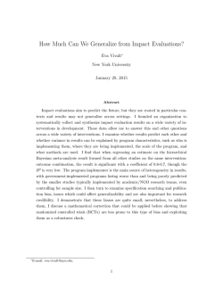
On the Relevance of Probability Distortions in the Extended
Warranties Market∗
[Preliminary and incomplete]
Jose Miguel Abito
Yuval Salant
January 28, 2015
Abstract
We study the reasons for high profits in the extended warranties market. Using data from
a big US consumer electronics retailer on extended warranty purchases between 1998 and 2004,
we estimate a model in which a profit-maximizing monopolistic seller offers extended warranties
to a population of risk-averse consumers who may distort failure probabilities. We find that
overweighting of failure probabilities is a relevant factor in determining economic outcomes in
this market: without probability overweighting, profits drop by 90% and consumer surplus
more than doubles. We also find that probability overweighting is affected by the environment
and is reduced with learning: there is less overweighting in online transactions than in in-store
transactions, and the likelihood of the same household buying an extended warranty is reduced
with experience.
∗
Abito:
University of Pennsylvania, Wharton School, Business Economics and Public Policy,
[email protected]. Salant: Northwestern University, Kellogg School of Management, Department of
Managerial Economics and Decision Sciences, [email protected]. Thanks: ...
1
1
Introduction
The market for extended warranties is highly profitable. Analysts estimate that extended warranties
accounted for almost half of BestBuy’s operating income in 2003, and that profit margins on these
warranties were about 50% to 60%. These margins were nearly 18 times the profit margins on the
products that the warranties covered.1 To likely avoid attention, BestBuy gradually reduced the
transparency of reporting on its extended warranty business since 2001. Around the same time,
concern about high profit margins on extended warranties led to a UK Competition Commission
investigation of their main consumer electronics retailers. Despite its efforts, the Commission did
not find evidence of abuse of dominance and instead attributed high profit margins to a “complex
monopoly situation,” the solution of which likely falls outside the scope of standard competition
policy (Baker and Siegelman, 2013).
One factor that may contribute to the high profitability of extended warranties lies in the way
these are marketed. In a brick and mortar store, a consumer is offered the extended warranty after
making the decision to buy the main product. At this stage, the seller potentially benefits from
close to monopoly pricing power because consumers may believe (or are convinced to believe) that
they cannot buy the same warranty elsewhere. In addition to this pricing power, there are demandrelated issues that potentially support high prices. An extended warranty is an insurance contract,
and buyers may be willing to pay a high premium to insure themselves against product failures.
Consumers’ high willingness-to-pay may be due to consumers’ aversion to risk, or due to mistakes
in evaluating the cost or likelihood of a failure. The recent empirical findings of Barseghyan et
al (2012) suggest that mistakes in the form of overweighting small probability events, rather than
“standard” risk aversion, are an important ingredient in consumers’ decision making when buying
insurance.2
Using extended warranty transactions from a large US consumer electronics retailer, we provide
empirical evidence that demand-side probability distortions in the form of overweighting and low
marginal sensitivity to changes in failures rate are important factors in driving the high profitability
in this market. Moreover, we argue that there is rationale and scope for intervention in the form
of well-designed consumer protection policies, and these have the potential to significantly improve
consumer welfare.
Our approach to studying the extended warranties market begins with providing evidence that
standard risk aversion is not likely to be a dominant factor in consumers’ decision to buy an extended
warranty. If it were, we would expect consumers’ likelihood of buying an extended warranty to be
significantly correlated with observables such as gender, age, and income (which to the best of our
knowledge do not affect the price of insurance in this market). We do not find indications of such
1
2
“The Warranty Windfall”, Business Week (Dec 19, 2004).
On the cost side, warranties cost very little to market, and fail very infrequently. It is possible, however, that failure
rates among those who buy extended warranties are higher than average due to moral hazard (conditional on buying
the warranty, consumers do not take good care of the product) and adverse selection (those with higher propensity
to break the product buy extended warranties), which then puts upward pressure on extended warranty prices.
2
correlations in our dataset.
We then proceed to specify a structural model of demand and supply that captures the main
features of the market. On the demand side, risk averse consumers decide whether to purchase the
warranty after making the decision to buy the main product. The warranty is a contract that fully
insures the buyer against the product failing. In deciding whether to buy the warranty, the buyer
approximates the cost of failure using the price paid for the product, but may make mistakes in
estimating the likelihood of failure and in incorporating this likelihood to the warranty’s value.
From the demand model, we separately identify and estimate the consumer’s degree of (standard) risk aversion and the distortion in evaluating failure rates. Our identification strategy relies
on how a household’s willingness-to-pay for an extended warranty varies across products that have
different costs of failure (i.e. loss from a product failure) but the same failure rates. We show
that a single-crossing condition of the willingness-to-pay function is sufficient to separately identify
standard risk aversion and probability distortions in this context. We provide examples of common
utility functions that satisfy the single-crossing property, including the one that we will use for
estimation.
On the supply side, we model the seller as a monopolist who prices the extended warranty
to maximize profit (given the price of the main product). We endow the retailer with monopoly
pricing power and investigate to what extent behavioral biases can influence monopoly prices. To
get a measure of the (expected) marginal cost of providing a warranty, we combine our supply
model with our demand estimates.
Our estimation results point to an important role of probability distortions in explaining extended warranty purchase behavior. First, we find substantial overweighting of failure rates below
15%. For example, a 5% failure rate is seen as if a product has a failure rate of 12% when an average
household is evaluating the warranty. Second, our estimate of standard risk aversion implies an
average willingness-to-pay that is close to actuarially fair rates, consistent with behavior of a risk
neutral consumer. We show that estimating a model that ignores probability distortions requires
extreme risk aversion to rationalize the data.
We perform counterfactual experiments to assess the impact of probability distortions on extended warranty prices, price-cost margins, and welfare. We find that the ratio of extended warranty
price to the main product price declines from 17% to 16%, with price-cost margins going down from
31% to 24% when we remove the bias. Removing the bias drastically reduces the fraction insured
from 39% to 7%.
The effect of removing the bias on welfare is ambiguous. Overweighting of failure rates inflates
consumers’ willingness-to-pay for the warranty, potentially leading to overinsurance relative to
the first best. On the other hand, market power leads to underinsurance. We estimate that the
deadweight-loss from overinsurance is larger than the deadweight-loss from underinsurance, and so
welfare increases when we remove the bias. Removing the bias leads to a welfare improvement of $9
million, or a 15% increase in welfare. More strikingly, consumer surplus improves by $219 million
3
(which represents more than a doubling of consumer surplus) when the retailer can no longer exploit
the bias. Finally profits go done from $267 million to $36 million, or an 85% decrease, in this case.
We conclude by exploring whether the bias is internal to the consumer or due to external
cues, and whether consumers adjust how they value the warranty based on past experience. If
probability distortions were influenced largely by one’s external environment and/or consumers
learn, then there is room and rationale for policy interventions to minimize the bias. Using our
panel data of households, we find substantially different purchasing behavior between online and
in-store transactions. Our best estimate suggests that the likelihood of purchasing an extended
warranty more than doubles from 12% to 29% when consumers interact with sales people in the
store. Moreover, prior experience with purchasing an extended warranty decreases the likelihood of
purchasing a warranty today by more than 25 percentage points, once we control for (unobserved)
persistent characteristics of the buyer.
The paper is organized as follows. The next section introduces the data and provides reducedform evidence against the view that risk aversion is the main driver for extended warranty purchase.
Section 3 presents the model and our identification strategy. Section 4 discusses estimation and
section 5 contains the results. We perform counterfactuals in section 6 and section 7 explores
whether there is rationale and scope for intervention.
2
Data
We use the INFORMS Society of Marketing Science (ISMS) Durables Dataset 1 which is a panel
data of household durable goods transactions from a major U.S. electronics retailer. The full sample
contains around 170,000 transactions made by almost 20,000 households across the retailer’s 1,176
outlets and its online store. Of these transactions, about 117,000 correspond to a specific product
that the household purchased in a given shopping trip. An extended warranty purchase is recorded
as a separate transaction. Transactions took place between December 1998 to November 2004. The
data also contains household characteristics including the buyer’s gender, the age and gender of
the head of the household, income group3 , and whether there are children in the household.
There are two data issues that we have to deal with. First, the data only tells us the product
subcategory (e.g. 9-16 inch TVs) for which the warranty is for. We restrict our sample to shopping
trips in which there is a clear one-to-one mapping between the extended warranty and the corresponding product. For example, we drop shopping trips involving a purchase of two 9-16 inch TVs
but only one extended warranty purchased for this subcategory. At the end, we lose about 2,000
observations for this reason.
Second, if a household does not purchase an extended warranty for a given product, we do
not observe the warranty’s price. To identify the warranty price in such cases, we match the
3
Income group is a number from 1-9 where 9 is the highest income group. The data documentation does not provide
information on how these groups are defined.
4
Table 1: By product category
AUDIO
DVS
IMAGING
MAJORS
MOBILE
MUSIC
P*S*T
PC HDWR
TELEVISION
VIDEO HDWR
WIRELESS
% bought EW
0.281
0.295
0.377
0.356
0.398
0.208
0.245
0.258
0.311
0.206
0.245
0.287
EW-Product price ratio
0.232
0.207
0.199
0.197
0.249
0.169
0.237
0.274
0.217
0.240
0.317
0.239
Obs
6450
1439
3001
864
5176
1189
3765
8773
6307
5828
1485
44277
nonwarranty transaction with a corresponding warranty transaction based on product ID and we
assign the observable price from the closest transaction date. We end up with a sample of about
45,000 observations.4
2.1
Attachment rates, prices, and approximate margins
Table 1 shows the fraction of consumers who bought extended warranties (henceforth, the attachment rate), and the ratio of the extended warranty price to the product price for each product
category. Attachment rates range from about 20% for items such as VCRs (VIDEO HDWR), music CDs and video games (MUSIC), to as high as about 40% for items like car stereos and speakers
(MOBILE). Warranties are priced at about 24% of the price of the insured product, on average.
We restrict our analysis to TVs due to availability of published failure rates from Consumer
Reports. Table 2 provides attachment rates, prices, ratio of extended warranty to product price,
published failure rates5 , and approximate price-cost margins, broken down by TV subcategory.
Attachment rates range from about 15% to 35%, with larger attachment rates for TVs that are 30
inches or higher (most expensive category). Similar to the other product categories, the warranty to
product price ratio is about 24% on average. To provide a rough estimate of the expected marginal
cost of servicing a warranty, we multiply the failure rates from Consumer Reports by the price of
the product. This estimate implies a price-cost margin of about 62 to 73%, which is close to what
is cited in the popular press. Note that we expect the seller in our dataset to have lower margins
due to issues like profit-sharing with third party providers of the warranty and commissions to sales
people.
4
We also drop observations where the price of the good is significantly less than the price of the warranty (less than
1,000 observations).
5
These failure rates come from Consumer Reports (see also table 6 (p. 22 ) of Wang, Ata and Islegen (2012)) which
gives the likelihood that a repair has to be made within 3 to 4 years of using the product. We construct lifetime
failure rates assuming the product lasts for 3.5 years.
5
9-16in
19-20in
25in
>30in
% bought
0.149
0.176
0.269
0.348
0.253
Table 2: By TV product type
TV price EW-TV price ratio Fail rate
122.989
0.284
0.072
173.973
0.240
0.065
244.923
0.220
0.069
812.533
0.219
0.076
421.092
0.235
0.070
Margin
0.729
0.710
0.643
0.619
0.667
Obs
422
1067
520
1229
3238
Notes: Fail rates are from Consumer Reports, assuming a 3-year lifetime and constant fail rate.
Margin = (EW price - CR fail rate × TV price)/EW price
2.2
Attachment rates by buyers’ characteristics
We examine the relationship between attachment rates and buyers’ characteristics in tables 3 and
4. Table 3 shows attachment rates broken down according to buyers’ (and households’) characteristics, while table 4 contains the results from a regression of extended warranty purchase on
these characteristics. All in all, these two tables suggest that buyers’ characteristics are not strong
predictors of extended warranties purchases.
Table 3 shows attachment rates broken down by gender of the buyer, gender and age of the head
of the household, whether income is above or below the median income category in the data, and
finally whether there is a child present in the household. Attachment rates do not significantly differ
across these groups. For example, around 27% of female buyers purchase the warranty compared
to 25% of male buyers. In terms of income, 25% of above median income households purchase the
warranty compared to 27% of below median income households. Although having a child seem to
decrease the likelihood of purchasing a warranty by 8 percentage points, this difference goes away
once we introduce controls.
Table 4 presents the results of regressing an extended warranty purchase dummy on buyers’
characteristics. The regressions include brand and subcategory fixed effects to account for average
differences in purchasing behavior across these dimensions. Focusing on the specification without
interaction terms (i.e. columns 2 and 3), none of the buyers’ characteristics are statistically significant predictors of extended warranty purchase, consistent with most of the raw means in table 3.
For example, the estimated effect of gender is just about 1% and is not statistically significant.
Turning to the estimates with interaction terms (i.e. columns 3 and 4), we again see that none of
the coefficients are statistically significant.
A wide literature in psychology and economics provides evidence that the above characteristics
we examine are correlated with risk aversion. (See Cohen and Einav (2007) and Dohmen et al
(2011) for recent studies, and Byrnes et al (1999) and Croson and Gneezy (2009) for surveys of
the literature.) For example, studies point to greater risk aversion among women than men. Read
through these lens, our results suggest that risk aversion is not the main factor driving extended
warranty purchase behavior.6
6
There is a concern that our coefficient estimates in table 4 confound the effect of risk aversion and risk type on
6
Table 3: Proportion of people who bought EW (TV)
Category
% bought Obs
Female
0.274
1076
Male
0.246
1860
Female (head of hh)
0.274
972
Male (head of hh)
0.245
1765
Above median income (category ≥ 5)
0.247
2446
Below median income (category < 5)
0.271
792
Over 50 (head of hh)
0.264
1865
Under 50 (head of hh)
0.239
1350
Has child in hh
0.234
881
No child in hh
0.316
531
Table 4: Regression of extended warranty purchase (TV) on household characteristics
Dependent variable: EW purchase dummy
Coeff
SE
Coeff
SE
Male (head)
-0.010 (0.026) -0.050
(0.132)
Age (head)
0.001 (0.001)
0.001
(0.001)
Income
-0.004 (0.006) -0.005
(0.009)
Has child in HH
-0.042 (0.030) -0.002
(0.046)
Male × Age
0.001
(0.002)
Male × Income
0.001
(0.012)
Male × Child
-0.061
(0.056)
Subcategory FE
Y
Y
Brand FE
Y
Y
No. obs (good-hh-trip)
1189
1189
Notes: Standard errors in parentheses are clustered at shopping trip level.
Significance level: ***1%, **5%, *10%
7
3
Model and identification
We proceed to study a model of the extended warranty market and estimate some of its parameters.
In the model, each consumer first decides which main product to buy, not taking into account the
potential purchase of the warranty. After finalizing this decision, the seller “surprises” the buyer,
and offers him to add-on an extended warranty to his purchase. The consumer then decides whether
to do so or not.7
The timing of the model and its sequential structure are motivated by how extended warranties
are sold in practice. In actual store settings, sales people usually offer this warranty to the buyer
after he finalizes his decision to purchase the corresponding product and is about to pay for it.8 It
seems unlikely that the buyer will revisit the costly decision to purchase the main product at this
stage. It also seems unlikely that when shopping for the main product, buyers seriously consider
the potential purchase of the extended warranty as no information about the warranty or its price
is usually provided before the decision to buy the product has been reached.
We focus on the second stage of the purchase process. At this stage, buyers decide whether to
purchase the warranty or not, which will be driven by their degree of risk aversion and probability
distortions. We can then solve for aggregate demand, and estimate the monopolist’s marginal cost
from his profit-maximizing pricing decision.
Starting with the buyer’s decision, a buyer’s value from purchasing the warranty is
VEW = u(W − t; r)
where W is the buyer’s wealth after buying the main product, t is the price of the warranty, and
u(·, r) is the consumer’s concave utility over wealth levels that is parameterized by r, the buyer’s
degree of risk aversion around W . Note that there is no deductible associated with using the
warranty, as is usually the case in extended warranty contracts.
purchase behavior (Cohen and Einav, 2007). That is, the same set of characteristics may affect the propensity of
buyers to break the product hence making them more likely to buy insurance (adverse selection). For example,
older people may perceive themselves as more likely to break the product whether or not this is in fact true.
Similarly, while propensity to break the product may be similar for males and females, males may underestimate
this propensity or females may overestimate it.
The concern is relevant if the effect of risk type on a given characteristics operates in the opposite direction and has
a similar magnitude to the effect of risk aversion. For example, if the increase in the likelihood of buying the
warranty due the higher risk aversion among women is non-zero, then it must be that women perceive themselves as
less likely than men to break the product such that this decreases the likelihood of warranty purchase by the same
magnitude. This complete offsetting seems unlikely to happen across all the characteristics we examine.
7
Note that the model does not specify how different sellers compete in the market. Following Ellison (2005), one can
extend the model to account for competition by assuming that firms advertise the prices of main products, but
buyers have to engage in costly search in order to figure out the warranty price. Such costly search guarantees that
each seller will benefit from monopoly power in pricing the warranty.
8
In the case of BestBuy, this timing is part of the company’s policy. See
https://www.extendingthereach.com/wps/PA VCorationFramework/resource?argumentRef=static&resourceRef=/files/Best Buy Vendor Selling Skills.pdf
8
The buyer’s value without the warranty is
VN W = ω(φ)E(u(W − X; r)) + (1 − ω(φ))u(W ; r)
where ω(φ) is the buyer’s perception of the objective failure probability φ, which increases in φ, and
X is the random cost of repair. Clearly, X ≤ A, where A is the price of the main product, because
the buyer can always buy a new product instead of fixing the existing one. Thus, the buyer’s value
without the warranty is bounded below by ω(φ)u(W − A; r) + (1 − ω(φ))u(W ; r). In what follows,
we will identify VN W with this lower bound, i.e., we will have:
VN W = ω(φ)u(W − A; r) + (1 − ω(φ))u(W ; r).9
The non-standard component in the model is the probability distortion function ω(·) that reflects
how the buyer assesses objective failure probabilities and how he uses them in making decisions.
There are at least two reasons for probability distortions. First, estimating failure probabilities
is not straightforward. This is because buyers usually have limited personal experience about the
failure of durable goods, and at the point of sale, the only other readily available information
source is the sales person whose incentives are to sell the warranty.10 Second, even if individuals
estimate failure probabilities correctly, Prospect Theory proposes that individuals incorporate these
probabilities in decision making by using decision weights. In particular, individuals tend to put
too much weight on low probability events, like the failure probability of a durable, hence increasing
the attractiveness of purchasing a warranty.
Individual heterogeneity is captured by choice shocks,
EW
and
NW ,
that additively affect VEW
and VN W . Assuming these shocks are iid Type I Extreme Value with scale parameter11 σ, we can
write the demand for extended warranties D(t; r, ω(φ), σ), in a unit mass population as follows:
D(t; r, ω(φ), σ) = Pr( N W − EW ≤ Ω(t; r, ω(φ), σ))
exp Ω(t; r, ω(φ), σ)
=
1 + exp Ω(t; r, ω(φ), σ))
where
Ω(t; r, ω(φ), σ) ≡
VEW − VN W
.
σ
(1)
Moving to the seller, he is a risk-neutral monopolist who prices the warranty to maximize profit
taking into account the demand for warranties and the cost of selling and servicing the warranty.
9
This implies that we likely underestimate ω and r because using a higher repair cost makes the purchase of the
warranty more attractive even without appealing to risk aversion and probability distortion.
10
“The company selling the warranty has the information on failure rates. You don’t....That’s not easy to find out.
Companies aren’t in the habit of telling you that their products fail 4 percent or 12 percent of the time. Failure
rates are usually low. Warranty companies know that. And they know, too, that consumers tend to think the
failure rate is higher.” (“Should I Buy an Extended Warranty”, New York Times, August 28, 2014).
11
The utility specification we will use in estimation imposes a specific normalization so we can identify a scale
parameter. This scale parameter is the inverse of the marginal utility of income.
9
This is motivated by consumers’ belief that searching for another main product or buying the
extended warranty elsewhere is costly.
Given a product priced at A with a failure probability φ, the seller’s expected marginal cost of
selling and servicing the warranty is c(A, φ). The seller chooses a price t to solve:
max(t − c(A, φ)) · D(t; r, ω(φ), σ)
t≥0
This is a standard monopoly pricing problem with the first-order condition:
1
t − c(A, φ)
=
t
|E(t; r, ω(φ), σ)|
(2)
where E(t; r, ω(φ), σ) is the price elasticity of demand for extended warranties.
3.1
Identification
The main challenge in identification is separately identifying risk aversion and the probability
weighting function given choice data on extended warranty purchases. Choice probabilities can be
inverted to get a measure of willingness-to-pay for the warranty and so we focus on how to uniquely
get (r, ω(·)) from willingness-to-pay.
Define a consumer by a pair (r, ω(φ)). The identification question boils down to whether
variation in willingness-to-pay allows us to differentiate consumers along the dimensions of (r, ω(φ)).
Our strategy relies on how willingness-to-pay vary with the loss that the consumer faces for different
products that have the same failure rate.
Fix the failure rate φ and let ω = ω(φ). Consider a buyer characterized by (r, ω) and define
her willingness-to-pay for an extended warranty on a good with underlying value A1 as t (A1 , r, ω),
where t (A1 , r, ω) is the extended warranty price t that solves
VEW (t, r) = VN W (A1 , r, ω) .
Consider a second buyer (r , ω ) such that r = r (or equivalently ω = ω) but
t A1 , r , ω
= t (A1 , r, ω) .
We say that r and ω are separately identified if there exists a second product with the same failure
rate but A2 = A1 that satisfies
t A2 , r , ω
= t (A2 , r, ω) .
The following property ensures this:
Property 1 (Single-crossing) For a utility function u(·), the implied willingness-to-pay t (·, r, ω)
10
satisfies the single-crossing property if
∂t(A,r,ω)
∂r
− ∂t(A,r,ω)
∂ω
strictly increases in A.
Figure 1: Identification: Single-crossing of
willingness-to-pay
Note: A1 > A2
Figure 1 graphically provides the intuition for sufficiency of single-crossing for identification.
The curve W T P (A1 , φ) is the combination of risk aversion parameters and probability weights that
give the same willingness-to-pay for a product with value A1 . If we only observed W T P (A1 , φ), then
we cannot separately identify r and ω since infinitely many pairs would rationalize the data. Now,
identification requires that if we look at a second good with value A2 = A1 but with the same failure
rate, then it must be that the willingness-to-pay curve W T P (A2 , φ) crosses W T P (A1 , φ) only at a
single point. We prove in the appendix that single-crossing holds for the Constant Absolute Risk
Aversion (CARA) case and for the second order Taylor approximation of any utility function. We
use the latter functional form in our estimation.
4
Estimation
Following Cohen and Einav (2007) and Barseghyan et al (2012), we use a second order Taylor
approximation of the utility function u(·) in estimating the model. The main benefit of using this
specification is that it does not require data on wealth.
The second order Taylor approximation of u(·) around W for some wealth deviation ∆ is given
11
by
u(W + ∆) ≈ u(W ) + u (W )∆ +
u (W ) 2
∆ .
2
Normalizing by u (W ) and letting r = −u (W )/u (W ), we obtain that12
u(W + ∆)
u(W )
r
≈
+ ∆ − ∆2 .
u (W )
u (W )
2
Using this specification to evaluate the difference in utility between purchasing an extended warranty (equation 1), we obtain that:
ω j Aj − tj + 2r (ω j A2j − t2 )
Ωj =
.
σ
Let qj be the observed attachment rate for product j. Our choice model implies13
log
ω j Aj − tj + 2r (ω j A2j − t2 )
qj
= Ωj =
.
1 − qj
σ
(3)
The decision weight ω j acts like a (non-additive) product effect. We decompose this effect as
follows:
ω j = ω(φj ) + ξ k(j) + η j .
(4)
where ω(·) is some unknown function of φ, ξ k(j) is a subcategory-level effect, and η j is a random
shock. The parameters ξ k(j) allow decision weights to vary between subcategories, thus capturing
the possibility that consumers may apply different decision weights for TVs of different sizes,
different projection technology, etc.
Using equation 3, we can express ω j ’s as functions of the unknown parameters (r, σ) and the
data:
ωj =
σΩj + tj + 2r t2j
Aj + 2r A2j
.
(5)
We construct moment conditions involving ω j to estimate r and σ.14 Once we have these parameters, we calculate ω j using equation 5. Our assumption regarding the error structure in equation 4
implies the following moment condition
E[ω j − ω j |φj = φj , k(j) = k(j ), Aj , Aj , tj , tj ] = 0
12
Strictly speaking, the Arrow-Pratt coefficient of risk aversion does not vary with income only for CARA utility.
A complication in linking Ωj to product-level attachment rates arises because A and t varies at the product level. If
we had infinite data, we can compute qj|A,t = Pr(di = 1|j(i) = j, A, t) and then invert this equation to get Ωj for
each pair (A, t). However, this is not our case. The best we can do is to aggregate across all price pairs (A, t) within
each product: qj = (A,t) Pr(di = 1|j(i) = j, A, t) Pr(A, t|j(i) = j) and then use the observed maximum value for A
and minimum value t.
14
Because of the large variation in prices across categories, we estimate separate scale
√ parameters for each
subcategory, and we allow for heteroskedasticity. Specifically we let σ k (A) = σ k A for subcategory k.
13
12
since ω j − ω j = η j − η j for j, j such that φj = φj and k(j) = k(j ). As long as failure rates
for any two products j and j belonging in the same subcategory are the same, decision weights
associated with extended warranties for these products will be equal, on average.
The last component we need to estimate is the marginal cost of the seller, c(A, φ). We assume
that c(A, φ) = µφA and estimate the parameter µ. The parameter µ absorbs factors that affect
cost such as sales commission, repair cost paid to a third party, the potential effect of moral hazard,
etc.
5
Results
5.1
Probability weighting and risk aversion
Figure 2 plots our estimate of the probability weighting function ω(·). We include a scatter plot
of the estimated product effects ω j ’s and a local linear fit. We also include a fit based on the
one-parameter Prelec (1998) function,
ω(φ) = exp[−(− log(φ))α ]
(6)
which is close but slightly less concave than the local linear fit. We estimate α = 0.685 with
bootstrapped standard error equal to 0.097.
Our estimates are in line with Prospect Theory. First, there is substantial overweighting of
small probabilities. For example, a product with a 5% failure rate is perceived as a product with
a 12% failure rate. Second, the degree of overweighting declines as failure rates increase.
Figure 2: Estimated weighting function
13
We estimate the risk aversion parameter r to be practically zero (≈ 10−5 with SE = 5 × 10−3 ).
We also estimate a risk aversion parameter under what we refer to as the standard model in which
ω(φ) = φ. We estimate this parameter to be equal to 0.013 (SE = 0.002).
To interpret our estimates, Table 5 presents the average willingness-to-pay (WTP)15 for an
extended warranty for a product worth $100 under various failure rates. Columns 2 and 3 present
the WTP using the estimated risk aversion parameter from the full model. In column 2, we compute
the WTP with our estimated weighting function, and in column 3, we impose ω(φ) = φ. Column
4 uses the estimated risk aversion parameter from the standard model in which ω(φ) = φ.
Columns 2, 3, and 4 illustrate that in the full model, the contribution of probability distortions
is much more significant than that of standard risk aversion. As column 3 shows, willingness-topay when there are no probability distortions is equal to the actuarially fair rate. In contrast, the
risk aversion parameter in Column 4 that comes from the standard model (i.e. without probability
distortions) requires a very high degree of aversion to risk in order to fit the data well. For example,
a consumer with this risk aversion parameter will only accept a 50-50 gamble with a loss of $30 if
the gain is at least $55.
Table 5: Average willingness-to-pay for EW on a good with value $100
Failure rate Model est Model est Standard est
ω
ω(φ) = φ
φ
0.01
5.805
1.000
1.621
0.02
7.844
2.001
3.209
0.03
9.427
3.001
4.767
0.04
10.785
4.002
6.297
0.05
12.003
5.002
7.799
0.06
13.123
6.003
9.276
0.07
14.173
7.003
10.728
0.08
15.166
8.004
12.157
0.09
16.116
9.004
13.563
0.10
17.029
10.004
14.949
5.2
Retailer’s cost
Expected marginal cost for an extended warranty for product j is µφj Aj . We estimate µ = 1.622
(SE = 0.479). This implies a back-of-the-envelope seller’s profit margin of 43%, because an extended
warranty is priced at about 20% of the price of the good, and the marginal cost of selling and
servicing the warranty is the product of µ = 1.623, the average failure rate 0.07 and the price of
the good. Estimates from the popular press indicate that BestBuy transfers about 40% of the price
15
The average WTPs are computed by setting the choice shocks,
weighting function, η j , to zero.
14
EW
and
NW ,
and the shock that enters the
of the warranty to the company that handles service, suggesting that BestBuy’s cost of selling the
warranty, mostly in the form of sales commission, is about 17%.
5.3
Robustness against different expected loss of the consumer
Our benchmark model uses the upper bound loss A to compute the value of not buying the extended
warranty. In table 6, we present the estimates of probability weighting and risk aversion when
we allow the expected loss to vary as a fraction of A. Clearly, by using the upper bound, we
underestimate the extent of the bias since the estimate of the Prelec parameter α decreases as we
decrease the loss. The estimate of standard risk aversion only becomes non-negligible once the
explanatory power of α is exhausted.
Table 6: Parameter estimates with varying expected cost
% of product price
r
Prelec α ω(0.05)
−5
100%
≈ 10
0.685
0.120
90%
≈ 10−5
0.631
0.135
80%
≈ 10−5
0.567
0.155
−5
70%
≈ 10
0.489
0.181
60%
≈ 10−5
0.396
0.213
−5
50%
≈ 10
0.284
0.255
40%
≈ 10−5
0.175
0.296
30%
≈ 10−5
0.105
0.326
−5
20%
≈ 10
0.071
0.339
0.343
10%
≈ 10−5
0.063
6
Counterfactuals
We are interested in quantifying the profit and welfare implications of probability distortions in
the extended warranty market. We thus focus on a counterfactual exercise in which we fix the
strategic environment, and study how optimal prices and quantities change when consumers do
not exhibit the bias. To the extent that the bias is triggered in part by the store environment or
can be alleviated with learning and experience, this exercise gives us quantitative insight on the
effectiveness of consumer protection policies, and informational campaigns.
We compare two settings. In the first, we use the estimated weighting function and estimated
risk aversion, and in the second we turn off the bias, i.e. set ω(φ) = φ but keep the same risk aversion
parameter. In each setting, we construct demand based on these estimates, on the product price A,
and on the failure rate φ, and derive optimal prices. This gives us two distributions of optimal prices:
one for biased consumers and another for unbiased consumers. In calculating optimal prices, we
use the risk aversion parameter estimated from the full model and also the one-parameter Prelec
(1998) function (i.e. equation 6 with estimated α = 0.685) as our weighting function whenever
relevant (biased consumers). These numbers depend on the product price A and failure rates
15
φ. First, we take the set of observed product prices and failure rates in our data, and generate
counterfactual distributions for the extended warranty-to-product price ratio, price-cost margins
and fraction insured. Second, we compute the price ratio, price-cost margins, fraction insured and
welfare measures for each φ ∈ {0.01, 0.02, ..., 0.15}, using the median TV price in our estimating
sample ($499.99).
6.1
Prices and profit margins
Figure 3 plots the density and cdf of the extended warranty price-to-product ratio with and without
the bias. Our model (with bias) predicts an average and median ratio of 17.03% and 14.31%, which
are slightly below the average and median ratio of 17.66% and 16.67% in the data. Removing the
bias shifts the distribution to the left and decreases the mean and median ratios to 15.58% and
12.78%, respectively.
Figure 4 plots the ratios as a function of failure rate. Ratios increase as failure rate increases
because marginal cost is increasing in failure rates. The ratio with the bias ranges from about 6.79%
to 27.68% and without the bias, from 5.33% to 27.38%. The gap between the two ratios tends to
decrease as the failure rate increases because the ratio with the bias increases at a decreasing rate
due to the concavity of the weighting function in the relevant region.
Figure 3: Counterfactual: Densities and cdfs of the ratio of
EW and TV price
16
Figure 4: Ratio of extended warranty and TV price
Figure 5 presents the effect of the bias on price-cost margins. With the bias, average and median
price-cost margins are 31.47% and 29.86%. The average and median price-cost margins from the
data (i.e. computed using our estimate of µ but with observed prices) are 31.09% and 39.11%.
Similar to extended warranty-to-product price ratio, removing the bias shifts the distribution to
the left, decreases the mean price-cost margin to 23.63%, and decreases the median to 19.24%.
These represent about a 25% and 36% reduction in the average and median price-cost margins.
The left panel of figure 6 plots the price-cost margins with and without the bias for various
failure rates. The right panel shows the percent reduction in price-cost margins from removing
the bias. With the bias, price-cost margins range from 12.08% to 76.09%, while without the bias,
the range is from 11.11% to 69.55%. The percent reduction in price-cost margins has an inverted
U-shape which peaks at about a failure rate of 6%. At this failure rate, removing the bias reduces
price-cost margins by about 26%.
17
Figure 5: Counterfactual: Densities and cdfs of price-cost
margins
Figure 6: TV price-cost margins
18
6.2
Quantity
The effect of the bias on the fraction of insured individuals is even more profound. Figure 7 plots
the density and cdf of the fraction insured with and without the bias. With the bias, the average
and median fraction insured are 38.59% and 41.10%, while the corresponding numbers in the data
are 32.42% and 31.58%. Without the bias, the average and median fraction of insured decreases to
6.75% and 5.92%. This reflects an 83% and 86% reduction in the average and median fraction of
consumers who buy the extended warranty.
Figure 7: Counterfactual: Densities and cdfs of fraction insured
6.3
Welfare
When consumers overweight failure probabilities, demand for extended warranties goes up. We
assume that the bias is “non-welfare-relevant”16 in the sense that the increase in consumers’
willingness-to-pay for the warranty due to the bias does not reflect a true increase in consumer
surplus and so will not be counted in computing welfare. The first best level of insurance is characterized by the intersection of the demand curve of unbiased consumers with the retailer’s marginal
cost t = µφA.
Figure 8 compares the fraction of insured individuals with and without the bias to the first-best
fraction insured. Clearly, there is substantial overinsurance with the bias relative to the first-best.
On the other hand, there is underinsurance without the bias relative to the first best, which is a
16
We borrow this term from Handel and Kolstad (2014).
19
consequence of monopoly pricing. The degree of overinsurance is non monotonic in the failure rate,
while the degree of underinsurance is decreasing.
Figure 8: Fraction insured
To get a realistic dollar equivalent measure for consumer surplus, profits and total welfare, we
assume that there are 30 million potential buyers of TV extended warranties.17
Consumer surplus increases when the bias is removed. There are two channels for this increase.
First, holding the extended warranty price constant, removing the bias shifts the demand curve
to the left and reduces the fraction insured. Consumers who now forgo buying the warranty are
exactly those who pay more than their unbiased willingness-to-pay, hence increasing consumer
surplus. We refer to this as the ripoff effect. Second, since extended warranty prices go down
without the bias, additional consumers would now like to buy the warranty, increasing the fraction
insured and consumer surplus. We refer to this as the price effect. Figure 9 illustrates these two
effects.
17
US TV shipments ranged from 37 million to 40 million over 2010 to 2013 (CNN, “With new TVs, size matters”,
June 26, 2013).
20
Figure 9: Two effects of removing the bias on Consumer Surplus
Figure 10 plots consumer surplus as a function of failure rate for the first best, and with and
without the bias. In the first best, consumer surplus ranges from $20 million to $268 million.
Without the bias, consumer surplus ranges from $7 million to $95 million and with the bias, it
ranges from -$193 million to -$48 million. At the mean failure rate of 7%, removing the bias
increases consumer surplus from -$185 million to $34 million, an improvement of $219 million.
Decomposing this increase in terms of the two effects, the ripoff effect is $207 million while the
price effect is $13 million.
21
Figure 10: Consumer Surplus
Figure 11 plots profits as a function of failure rates. Profits are zero in the first best while profits
range from $7 million to $106 million when there is no bias. When there is bias, profits range from
$52 million to $352 million. At the mean failure rate, profits fall from $246 million with the bias,
to $36 million without the bias, a decrease of about 85%. Most of the profits when consumers are
biased comes from the surplus extracted from consumers who would not have bought the warranty
otherwise, i.e. the ripoff effect.
22
Figure 11: Profits
We now turn to the effect of removing the bias on total welfare. The effect depends on whether
the quantity insured with the bias, q bias , is below or above the first best quantity, q F B . Welfare
unambiguously decreases when we remove the bias if q F B ≥ q bias since the bias actually brings
us closer to the first best quantity from below. On the other hand, if q F B < q bias , the effect
of removing the bias is ambiguous. In this case, one needs to compare the deadweight-loss from
overinsurance with the deadweight-loss from underinsurance. Figure 12 illustrates the comparison
of deadweight-losses for q F B < q bias .
23
Figure 12: Comparing deadweight-loss when q F B < q bias
Figure 13 plots total welfare as a function of failure rates. For failure rates below 6%, removing
bias decreases welfare by about $0.9 million to $65 million. However for failure rates above 6%,
removing the bias increases welfare by about $9 million to $22 million. At the mean failure rate,
welfare with the bias is $61 million while without the bias, welfare is $70 million. This reflects an
improvement of $9 million from removing the bias, or a 15% increase in welfare. Deadweight-loss
due to overinsurance is $111 million while deadweight-loss due to underinsurance is $82 million.
24
Figure 13: Total Welfare
To summarize our welfare analysis, although the effect of the bias on welfare is a priori ambiguous, we do find that policies that can successfully reduce the bias are welfare-enhancing. Moreover,
there is overwhelming reason to adopt such policies as the impact of the bias on consumer welfare
is substantial.
7
Is there room for intervention?
The counterfactual margin analysis in the previous section quantifies the potential role of consumer
protection policy to reduce margins in the extended warranties market. However, efficacy of such
an intervention depends on what drives consumer bias in the first place. Is the bias inherent to the
decision maker or is it mostly influenced by her external environment, say, due to manipulations
or sales tactics implemented by the seller? Is the bias intrinsic and deeply built-in in consumer
behavior, or can experience and education about the product decrease the extent of the bias? If the
source of bias is external and/or consumers learn, then there is room for well-designed consumer
protection policy.18
To gain insight on the source of the bias, we first examine consumer behavior in transactions
made online and in the store. We use the full dataset in the succeeding analysis to increase our
sample size and range of products. Table 7 compares raw attachment rates online vs in-store. The
in-store attachment rates are close to the overall attachment rate (29%), while online attachment
18
Baker and Siegelman (2013) explore some regulatory responses in this market.
25
Table 7: Online vs In-store extended warranty purchases
Mean Std dev No obs
All
0.287 0.452
44304
In-store 0.289 0.453
43876
Online
0.042 0.201
428
Notes: Observation are at the good-hh-trip level
Table 8: Regression of extended warranty purchase on shopping mode
Dependent variable: EW purchase dummy
I
II
III
IV
V
In-store?
0.247*** 0.200*** 0.180*** 0.175*** 0.166***
(0.022)
(0.027)
(0.027)
(0.027)
(0.027)
Household FE
N
Y
Y
Y
Y
Subcategory FE N
N
Y
Y
Y
Brand FE
N
N
N
Y
Y
Month FE
N
N
N
N
Y
Year FE
N
N
N
N
Y
No. obs
44304
44304
44304
44304
44304
(good-hh-trip)
No. HHs
17158
17158
17158
17158
17158
Notes: Standard errors in parentheses are clustered at shopping trip level.
Significance level: ***1%, **5%, *10%
rates are significantly lower at 4%. Taken as is, this represents a sevenfold (an increase of about 25
percentage points) nudge to buy extended warranties when in the store. The number of transactions
is way lower online than in the store so one might worry that the difference is driven by other factors
such as which consumers buy online, what products are bought, etc.
Exploiting the panel data structure of our dataset, we explore various regressions in Table 8 to
examine the robustness of the in-store effect on purchases. The first model (I) does not include any
controls so it gives the same numbers as table 7. The next models turn on various fixed effects.
Subcategory and brand fixed effects allow us to soak up any differences in mean purchasing behavior
induced by the nature of the product. We also include household, month and year fixed effects as
further controls.
We see a drop of the effect of in-store purchases as we include more fixed effects. Including
just a household fixed effects reduces the effect by about 5 percentage points. The reduction in the
effect is much larger when including product-related fixed effects. Including all of the fixed effects
lead to a reduction in the effect from 25 percentage points to 17. Being in the store leads to a jump
in attachment rates from 12% to 29%, which is more than a twofold nudge.
As an additional robustness check, table 9 contains the result of regressing the extended warranty
purchase dummy on shopping mode but broken down by product category. The first two columns
come from a simple OLS regression without additional controls. The middle two columns include the
household characteristics in the data as controls. Finally the last two columns include a household
26
Table 9: Regression of extended warranty purchase on shopping mode broken down by product
category
Dependent variable: EW purchase dummy
OLS
se
Obs OLS with char se
Obs FE (HH) se
Television
0.31∗∗∗ (0.08) 6307 0.32∗∗
(0.14) 2360 0.22
(0.20)
∗∗∗
∗
Audio
0.16
(0.05) 6450 0.12
(0.07) 2517 0.07
(0.10)
Mobile
0.40∗∗
(0.19) 5176 0.37
(0.28) 1883 .
.
P*S*T
0.23∗∗∗ (0.06) 3765 0.23∗∗∗
(0.08) 1519 0.19∗
(0.11)
Imaging
0.36∗∗∗ (0.07) 3001 0.39∗∗∗
(0.12) 1197 .
.
(0.08) 3471 0.03
(0.11)
PC Hardware 0.18∗∗∗ (0.05) 8773 0.09
Music
0.16∗
(0.09) 1189 0.20
(0.15) 469
0.30
(0.24)
∗∗∗
∗∗∗
∗
Video
0.21
(0.04) 5828 0.22
(0.07) 2151 0.17
(0.09)
DVS
0.05
(0.23) 1439 0.34
(0.46) 586
0.50∗
(0.28)
∗∗
Wireless
0.25
(0.18) 1485 0.27
(0.31) 483
0.57
(0.25)
Notes:
Significance level: ***1%, **5%, *10%
fixed effect. There is significant variation in the effect of in-store purchases across the product
categories but overall, the effect remains large. The effect survives even if we include household
characteristics. Although we lose statistical significance once we include household fixed effects
due to a small number of observations, the magnitudes are roughly the same across the different
regression models.
We now explore how experience with buying extended warranties in the past affects the likelihood of purchasing a warranty in the present. Table 10 contains the results of regressions of
extended warranty purchase for a given product on whether an extended warranty was purchased
in prior transactions on any other products. Our most preferred specification includes household,
subcategory, brand, month and year fixed effects. Our results provide evidence of learning.19 Experience with extended warranties in the past decreases the likelihood of buying a warranty in the
present by 25 percentage points, i.e. attachment rates go down from 29% to just 4%. We also
measure experience in terms of the number of extended warranties bought in the past for any other
good. We find that buying one extended warranty in the past decreases likelihood of buying an
extended warranty today by 7 percentage points.
To conclude, we find that distortions in the online market place are much smaller suggesting
that some of the distortion must come from external forces. This finding is consistent with the
view that aggressive sales tactics in the store is a major factor driving purchasing behavior and
consumer bias. Moreover, we find that experience with extended warranties in the past has a
significant impact on the likelihood of purchase in the present, which is a sign of learning about
the value of the extended warranty.
19
Interestingly, when household fixed effects are not included, we estimate a positive effect of past purchasing
behavior on the likelihood of buying today, contrary to learning. This reflects the classic problem of disentangling
unobserved persistent heterogeneity and state dependence.
27
Table 10: Regression of current EW purchase behavior on past EW purchase
Dependent variable: Buy EW today?
I
II
III
IV
V
Bought EW before?
0.238*** 0.235*** -0.253*** -0.253***
(0.007)
(0.007)
(0.020)
(0.020)
No. of EW bought before
-0.068***
(0.007)
In-store?
0.180*** 0.173***
(0.037)
(0.036)
Household FE
N
N
Y
Y
Y
Subcat & brand FE
N
Y
Y
Y
Y
Month & Yr FE
Y
Y
Y
Y
Y
No. obs
18811
18811
18811
18811
18811
(good-hh-trip)
No. HHs
7842
7842
7842
7842
7842
Notes: Standard errors in parentheses are clustered at shopping trip level. Dependent variable
refers to a given product while “Bought” dummy regressor refers to buying an EW for any product
in the past. Model V uses the number of extended warranties bought on any other product before
as a regressor. Significance level: ***1%, **5%, *10%
References
[[TBD]]
28
Appendix
Utility functions that satisfy property 1 (single-crossing)
The following lemma is a useful extension for determining whether single-crossing holds for a given
function. We use it throughout when we show that a given utility function satisfies property 1.
Lemma 1 The function t (·, r, ω) satisfies the single-crossing property if and only if for any function
g(·) such that
dg(t(A,r,ω))
dt
= 0,
t (A1 , r, ω) = t A1 , r , ω
t (A2 , r, ω) = t A2 , r , ω ,
for some A1 and A2 such that A1 = A2 , then
∂g(t(A,r,ω))
∂ω
− ∂g(t(A,r,ω))
∂r
is strictly increasing in A for any transformation g (·) such that
g (t (A1 , r, ω)) = g t A1 , r , ω
g (t (A2 , r, ω)) = g t A2 , r , ω
and
dg(t(A,r,ω))
dt
= 0.
Proof. Note:
∂g(t(A,r,ω))
∂r
∂g(t(A,r,ω))
∂ω
=
dg(t(A,r,ω)) ∂t(A,r,ω)
dt
∂r
dg(t(A,r,ω)) ∂t(A,r,ω)
dt
∂ω
=
∂t(A,r,ω)
∂r
∂t(A,r,ω)
∂ω
by chain-rule. The rest follows from the single-crossing property.
CARA utility
Suppose
u(C) = −e−rC .
Here, we have
Ω = VEW − VN W
= −e−r(W −t) + ωe−r(W −A) + (1 − ω)e−rW .
Willingness-to-pay is given by
t(A, r, ω) =
log(ωerA + 1 − ω)
.
r
29
(7)
Define the transformation
g (t (A, r, ω)) =
∂t(A,r,ω)
∂A
.
∂ 2 t(A,r,ω)
2
∂A
(8)
Using this transformation and the formula for willingness-to-pay (equation 7), we can compute
∂
∂A
∂g(t(A,r,ω))
∂ω
∂g(t(A,r,ω))
∂r
=−
r2 erA (1 − ω + ωerA )
<0
(1 − ω)[1 − ω(1 − erA (1 − rA))]2
and therefore the CARA utility function satisfies property 1 after applying lemma 1.
Second order Taylor approximation
For the 2nd order Taylor approximation, willingness-to-pay is given by
t (A, r, ω) =
1
r
r
−1 + 1 + 2rω A + A2
2
1/2
.
We use the same transformation as in the CARA case (i.e. equation 8). This gives
∂
∂A
∂g(t(A,r,ω))
∂ω
∂g(t(A,r,ω))
∂r
=−
3 (1 + Ar)2 1 + 2Arω + A2 r2 ω
r2 (1 − ω)3
and thus, property 1 is satisfied after using lemma 1.
30
<0