
How Much Can We Generalize from Impact Evaluations?
How Much Can We Generalize from Impact Evaluations?
Eva Vivalt∗
New York University
January 28, 2015
Abstract
Impact evaluations aim to predict the future, but they are rooted in particular contexts and results may not generalize across settings. I founded an organization to
systematically collect and synthesize impact evaluation results on a wide variety of interventions in development. These data allow me to answer this and other questions
across a wide variety of interventions. I examine whether results predict each other and
whether variance in results can be explained by program characteristics, such as who is
implementing them, where they are being implemented, the scale of the program, and
what methods are used. I find that when regressing an estimate on the hierarchical
Bayesian meta-analysis result formed from all other studies on the same interventionoutcome combination, the result is significant with a coefficient of 0.6-0.7, though the
R2 is very low. The program implementer is the main source of heterogeneity in results,
with government-implemented programs faring worse than and being poorly predicted
by the smaller studies typically implemented by academic/NGO research teams, even
controlling for sample size. I then turn to examine specification searching and publication bias, issues which could affect generalizability and are also important for research
credibility. I demonstrate that these biases are quite small; nevertheless, to address
them, I discuss a mathematical correction that could be applied before showing that
randomized controlled trials (RCTs) are less prone to this type of bias and exploiting
them as a robustness check.
∗
E-mail: [email protected].
1
1
Introduction
In the last few years, impact evaluations have become extensively used in development eco-
nomics research. Policymakers and donors typically fund impact evaluations precisely to figure out
how effective a similar program would be in the future, to guide their decisions on what course
of action they should take. However, it is not yet clear how much we can extrapolate from past
results or under which conditions. Further, there is some evidence that even a similar program,
in a similar environment, can yield different results. For example, Bold et al. (2013) carry out
an impact evaluation of a program to provide contract teachers in Kenya; this was a scaled-up
version of an earlier program studied by Duflo, Dupas and Kremer (2012). The earlier intervention
studied by Duflo et al. was implemented by an NGO, while Bold et al. compared implementation
by an NGO and the government. While Duflo et al. found positive effects, Bold et al. showed
significant results only for the NGO-implemented group. The different findings in the same country
for purportedly similar programs point to the substantial context-dependence of impact evaluation
results. Knowing this context-dependence is crucial in order to understand what we can learn from
any impact evaluation.
While the main reason to examine generalizability is to aid interpretation and improve predictions, it would also help to direct research attention to where it is most needed. If generalizability
were higher in some areas, fewer papers would be needed to understand how people would behave
in a similar situation; conversely, if there were topics or regions where generalizability was low,
it would call for further study. With more information, researchers can better calibrate where to
direct their attentions to generate new insights.
It is well-known that impact evaluations only happen in certain contexts. For example, Figure
1 shows a heat map of the geocoded impact evaluations in the data used in this paper overlaid by
the distribution of World Bank projects (black dots). Both sets of data are geographically clustered, and whether or not we can reasonably extrapolate from one to another depends on how much
heterogeneity there is in treatment effects. Allcott (2012) recently showed that site selection bias
was an issue for randomized controlled trials (RCTs) on a firm’s energy conservation programs.
Microfinance institutions that run RCTs and hospitals that conduct clinical trials are also selected
(Allcott, 2012), and World Bank projects that receive an impact evaluation are different from those
2
Figure 1: Growth of Impact Evaluations and Location Relative to Programs
The figure on the left shows a heat map of the impact evaluations in AidGrade’s database overlaid by black dots
indicating where the World Bank has done projects. While there are many other development programs not done
by the World Bank, this figure illustrates the great numbers and geographical dispersion of development programs.
The figure on the right plots the number of studies that came out in each year that are contained in each of three
databases described in the text: 3ie’s title/abstract/keyword database of impact evaluations; J-PAL’s database of
affiliated randomized controlled trials; and AidGrade’s database of impact evaluation results data.
that do not (Vivalt, Ambrose and Lopez, 2014). Others have sought to explain heterogeneous
treatment effects in meta-analyses of specific topics (e.g. Saavedra and Garcia, 2013, among many
others for conditional cash transfers), or to argue they are so heterogeneous they cannot be adequately modelled (e.g. Deaton, 2011; Pritchett and Sandefur, 2013).
Impact evaluations are still exponentially increasing in number and in terms of the resources
devoted to them. The World Bank recently received a major grant from the UK aid agency DFID
to expand its already large impact evaluation works; the Millennium Challenge Corporation has
committed to conduct rigorous impact evaluations for 50% of its activities, with “some form of
credible evaluation of impact” for every activity (Millennium Challenge Corporation, 2009); and
the U.S. Agency for International Development is also increasingly invested in impact evaluations,
coming out with a new policy in 2011 that directs 3% of program funds to evaluation.1
Yet while impact evaluations are still growing in development, a few thousand are already
complete. Figure 1 plots the explosion of RCTs that researchers affiliated with J-PAL, a center for development economics research, have completed each year; alongside are the number of
development-related impact evaluations released that year according to 3ie, which keeps a direc1
While most of these are less rigorous “performance evaluations”, country mission leaders are supposed to identify
at least one opportunity for impact evaluation for each development objective in their 3-5 year plans (USAID, 2011).
3
tory of titles, abstracts, and other basic information on impact evaluations more broadly, including
quasi-experimental designs; finally, the dashed line shows the number of papers that came out in
each year which are included in AidGrade’s database of impact evaluation results, which will be
described more shortly.
To summarize, while we do impact evaluation to figure out what will happen in the future,
many issues have been raised about how well we can extrapolate from past impact evaluations,
and despite the importance of the topic, previously we were unable to do little more than guess or
examine the question in narrow settings as we did not have the data. Now we have the opportunity
to address speculation, drawing on a large, unique dataset of impact evaluation results.
I founded a non-profit organization dedicated to gathering this data. That organization, AidGrade, seeks to systematically understand which programs work best where, a task that requires
also knowing the limits of our knowledge. To date, AidGrade has conducted 20 meta-analyses
and systematic reviews of different development programs.2 Data gathered through meta-analyses
are the ideal data to answer the question of how much we can extrapolate from past results, and
since data on these 20 topics were collected in the same way, coding the same outcomes and other
variables, we can look across different types of programs to see if there are any more general trends.
Currently, the data set contains 587 papers on 196 narrowly-defined intervention-outcome combinations, with the greater database containing 14,945 estimates.
The data further allow me to examine a second set of questions revolving around specification searching and publication bias. Specification searching refers to the practice of researchers
artificially selecting results that meet the criterion for being considered statistically significant,
biasing results. It has been found to be a systematic problem by Gerber and Malhotra in the
political science and sociology literature (2008a; 2008b); Simmons and Simonsohn (2011) and Bastardi, Uhlmann and Ross (2011) in psychology; and Brodeur et al. (2012) in economics. I look
for evidence of specification searching and publication bias in this large data set, both for its own
importance as well as because it is possible that results may appear to be more “generalizable”
merely because they suffer from a common bias.
I pay particular attention to randomized controlled trials (RCTs), which are considered the
2
Throughout, I will refer to all 20 as meta-analyses, but some did not have enough comparable outcomes for
meta-analysis and became systematic reviews.
4
“gold standard” in the sciences and on which development economics has increasingly relied. It is
possible that the method may reduce specification searching due to its emphasis on rigor or the
increased odds of publication independent of results. It is also possible that RCTs may be done in
more selected settings, leading to results not generalizing as well. I will shed light on both of these
potential issues.
The outline of this paper is as follows. First, I define generalizability, present some basic statistics about it, and use k-fold cross-validation to check what kinds of study characteristics can help
predict the results better than placebo data. I also conduct leave-one-out hierarchical Bayesian
meta-analyses of all but one result within an intervention-outcome combination and check to what
extent these meta-analysis results, which theoretically might provide the best estimates of a given
program’s effects, predict the result left out. Since some of the analyses will draw upon statistical
methods not commonly used in economics, I will use the concrete example of conditional cash transfers (CCTs), which are relatively well-understood and on which many papers have been written,
to elucidate the issues.
Regarding specification searching, I first conduct caliper tests on the distribution of z-statistics,
seeing whether there is a disproportionate number of papers just above the threshold for statistical
significance compared to those just below the threshold. The data contain both published papers
and unpublished working papers, and I examine how much publication bias there appears to be
for results that are significant. The bias towards novel findings can also serve as a measure of how
much economists typically think results generalize: if they believe that papers do not generalize
much, every paper on an intervention should be equally likely to be published regardless of whether
it covers outcome variables already addressed by previous studies. I test this hypothesis. Finally,
I examine whether papers’ findings appear to be related to their publication order. In particular,
I find that later papers within intervention-outcome combinations sometimes seem to report more
“dramatic” results, i.e. results that lie further from the mean.
After examining how much these biases are present, I discuss how one might correct for them
when considering generalizability. There is a simple mathematical adjustment that could be made
if one were willing to accept the constraints of a fixed effects meta-analysis model.3 However, I
show this would not be an appropriate model for these data. Instead, I turn to using RCTs, which
3
In particular, Simonsohn et al. (2014) make the assumption of fixed effects.
5
I show do not suffer as much from these biases, as a robustness check.
While this paper focuses on results for impact evaluations of development programs, this is only
one of the first areas within economics to which these kinds of methods can be applied. In many of
the sciences, knowledge is built through a combination of researchers conducting individual studies
and other researchers synthesizing the evidence through meta-analysis. This paper begins that
natural next step.
2
Theory
2.1
Heterogeneous Treatment Effects
I model treatment effects as potentially depending on the context of the intervention. Each
impact evaluation is on a particular intervention and covers a number of outcomes. The relationship
between an outcome, the inputs that were part of the intervention, and the context of the study
is complex. In the simplest model, we can imagine that context can be represented a “contextual
variable”, C, such that:
Zj “ α ` βTj ` δCj ` γTj Cj ` εj
(1)
where j indexes the individual, Z represents the value of an aggregate outcome such as “enrollment
rates”, T indicates being treated, and C represents a contextual variable, such as the type of agency
that implemented the program.4
In this framework, a particular impact evaluation might explicitly estimate:
Zj “ α ` β 1 Tj ` εj
(2)
but, as Equation 1 can be re-written as Zj “ α ` pβ ` γCj qTj ` δCj ` εj , what β 1 is really capturing
is the effect β 1 “ β ` γC. When C varies, unobserved, in different contexts, the variance of β 1
increases.
This is the simplest case. One can imagine that the true state of the world has “interaction
effects all the way down”.
4
Z can equally well be thought of as the average individual outcome for an intervention. Throughout, I take high
values for an outcome to represent a beneficial change unless otherwise noted; if an outcome represents a negative
characteristic, like incidence of a disease, its sign will be flipped before analysis.
6
Interaction terms are often considered a second-order problem. However, that intuition could
stem from the fact that we usually look for interaction terms within an already fairly homogeneous
dataset - e.g. data from a single country, at a single point in time, on a particularly selected sample.
Not all aspects of context need matter to an intervention’s outcomes. The set of contextual
variables can be divided into a critical set on which outcomes depend and an set on which they do
not; I will ignore the latter. Further, the relationship between Z and C can vary by intervention or
outcome. For example, school meals programs might have more of an effect on younger children,
but scholarship programs could plausibly affect older children more. If one were to regress effect size
on the contextual variable “age”, we would get different results depending on which intervention
and outcome we were considering. Therefore, it will be important in this paper to look only at a
restricted set of contextual variables which could plausibly work in a similar way across different
interventions. Additional analysis could profitably be done within some interventions, but this is
outside the scope of this paper.
Generalizability will ultimately depend on the heterogeneity of treatment effects. The next
section formally defines generalizability for use in this paper.
2.2
Generalizability: Definitions and Measurement
Definition 1 Generalizability is the ability to predict results accurately out of sample.
Definition 2 Local generalizability is the ability to predict results accurately in a particular
out-of-sample group.
Any empirical work, including this paper, will only be able to address local generalizability. However, I will argue we should not be concerned about this. First, the meta-analysis
data were explicitly gathered using very broad inclusion criteria, aiming to capture the universe
of studies. Second, by using a large set of studies in various contexts and repeatedly leaving out
some of the studies when generating predictions, we can estimate the sensitivity of results to the
inclusion of particular papers. In particular, as part of this paper I will systematically leave out
one of the studies, predict it based on the other studies, and do this for each study, cycling through
the studies. As a robustness check I do this for different subsets of the data.
7
There are several ways to measure predictive power. Most measures of predictive power rely on
building a model on a “training” data set and estimating the fit of that model on an out-of-sample
“test” data set, or estimating on the same data set but with a correction. Gelman et al. (2013)
provides a good summary. I will focus on one of these methods - cross-validation. In particular,
I will use the predicted residual sum of squares (PRESS) statistic, which is closely related to the
mean squared error and can also be used to generate an R2 -like statistic. Specifically, to calculate
it one follows this procedure:
1. Start at study i “ 1 within each intervention-outcome combination.
2. Generate the predicted value of effect size Yi , Ypi , by building a model based on Y´i , the effect
sizes for all observations in that intervention-outcome except i. For example, regress Y´i “
α`βC´i `ε, where C represents a predictor of interest, and then use the estimated coefficients
to predict Ypi . Alternatively, generate Ypi as the meta-analysis result from synthesizing Y´i .
3. Calculate the squared error, pYi ´ Ypi q2 .
4. Repeat for each i ‰ 1.
5. Calculate PRESS “
ř
n pYi
´ Ypi q2
To aid interpretation, I also calculate the PRESS statistic for placebo data in simulations. The
models for predicting Yi are intentionally simple, as both economists and policymakers do not tend
to build complicated models of the effect sizes when drawing inferences from past studies. First,
I simply see if interventions, outcomes, intervention-outcomes, region or implementer have any
explanatory power in predicting the resultant effect size. I also try using the meta-analysis result
M´i , obtained from synthesizing the effect sizes Y´i , as the predictor of Yi . This makes intuitive
sense; we are often in the situation of wanting to predict the effect size in a new context from a
meta-analysis result.
When calculating the PRESS statistic, I correct the results for attenuation bias using a firstorder approximation described in Gelman et al. (2013) and Tibshirani and Tibshirani (2009).
y “ CV ´ CV.
Ě
Representing the cross-validation squared error pYi ´ Ypi q2 as CV, bias
8
While predictive power is perhaps the most natural measure of generalizability, I will also show
results on how much impact evaluation results correlate with each other. The difference between
correlation and predictive power is clear: it is similar to the difference between an estimated
coefficient and an R2 . Impact evaluation results could be correlated so that regressing Yi on
explanatory variables like M´i could result in a large, significant coefficient on the M´i term while
still having a low R2 . Indeed, this is what we will see in the data.
To create the meta-analysis result M´i , I use a hierarchical Bayesian random effects model with
an uninformative prior, as described in the next section on meta-analysis.
2.3
Models Used in Meta-Analyses
This paper uses meta-analysis as a tool to synthesize evidence.
As a quick review, there are many steps in a meta-analysis, most of which have to do with the
selection of the constituent papers. The search and screening of papers will be described in the
data section; here, I merely discuss the theory behind how meta-analyses combine results.
One of two main statistical models underlie almost all meta-analyses: the fixed-effect model
or the random-effects model. Fixed-effect models assume there is one true effect of a particular
program and all differences between studies can be attributed simply to sampling error. In other
words:
Yi “ θ ` ε i
(3)
where θ is the true effect and εi is the error term.
Random-effects models do not make this assumption; the true effect could potentially vary from
context to context. Here,
Yi “ θi ` εi
“ θ¯ ` ηi ` εi
(4)
(5)
where θi is the effect size for a particular study i, θ¯ is the mean true effect size, ηi is a particular
study’s divergence from that mean true effect size, and εi is the error.
When estimating either a fixed effect or random effects model through meta-analysis, a choice
9
must be made: how to weight the studies that serve as inputs to the meta-analysis. Several
weighting schemes can be used, but by far the most common to use are inverse-variance weights.
As the variance is a measure of how certain we are of the effect, this ensures that those results about
which we are more confident get weighted more heavily. The variance will contain a between-studies
term in the case of random effects. Writing the weights as W , the summary effect is simply:
řk
M “ ři“1
k
W i Yi
(6)
i“1 Wi
with standard error
b
řk 1
i“1
Wi
.
To build a hierarchical Bayesian model, I first assume the data are normally distributed:
Yij |θi „ N pθi , σ 2 q
(7)
where j indexes the individuals in the study. I do not have individual-level data, but instead can
use sufficient statistics:
Yi |θi „ N pθi , σi2 q
(8)
where Yi is the sample mean and σi2 the sample variance. This provides the likelihood for θi .
I also need a prior for θi . I assume between-study normality:
θi „ N pµ, τ 2 q
(9)
where µ and τ are unknown hyperparameters.
Conditioning on the distribution of the data, given by Equation 8, I get a posterior:
θi |µ, τ, Y „ N pθˆi , Vi q
where
θˆi “
Yi
σi2
1
σi2
`
`
µ
τ2
1
τ2
, Vi “
1
σi2
1
`
(10)
1
τ2
(11)
I then need to pin down µ|τ and τ by constructing their posterior distributions given noninformative priors and updating based on the data. I assume a uniform prior for µ|τ , and as the
10
Yi are estimates of µ with variance pσi2 ` τ 2 q, obtain:
µ|τ, Y „ N pˆ
µ, Vµ q
where
ř
µ
ˆ“
For τ , note that ppτ |Y q “
Yi
i σi2 `τ 2
ř
1
i σi2 `τ 2
(12)
ppµ,τ |Y q
ppµ|τ,Y q .
, Vµ “
ÿ
1
i
1
σi2 `τ 2
(13)
The denominator follows from Equation 12; for the numer-
ator, we can observe that ppµ, τ |Y q is proportional to ppµ, τ qppY |µ, τ q, and we know the marginal
distribution of Yi |µ, τ :
Yi |µ, τ „ N pµ, σi2 ` τ 2 q
(14)
I use a uniform prior for τ , following Gelman et al. (2005). This yields the posterior for the
numerator:
ppµ, τ |Y q9ppµ, τ q
ź
N pYi |µ, σi2 ` τ 2 q
(15)
i
Putting together all the pieces in reverse order, I first simulate τ , then generate ppτ |Y q using
τ , followed by µ and finally θi .
Unless otherwise noted, I rely on this hierarchical Bayesian random effects model to generate
meta-analysis results.
3
Data
This paper uses a database of impact evaluation results collected by AidGrade, a U.S. non-
profit that I founded in 2012. AidGrade focuses on gathering the results of impact evaluations and
analyzing the data, including through meta-analysis. Its data on impact evaluation results were
collected in the course of its meta-analyses from 2012-2014 (AidGrade, 2014).
AidGrade’s meta-analyses follow the standard stages: (1) topic selection; (2) a search for relevant papers; (3) screening of papers; (4) data extraction; and (5) data analysis. In addition, it
pays attention to (6) dissemination and (7) updating of results. Here, I will discuss the selection of
papers (stages 1-3) and the data extraction protocol (stage 4); more detail is provided in Appendix
B.
11
3.1
Selection of Papers
The interventions that were selected for meta-analysis were selected largely on the basis of there
being a sufficient number of studies on that topic. Five AidGrade staff members each independently
made a preliminary list of interventions for examination; the lists were then combined and searches
done for each topic to determine if there were likely to be enough impact evaluations for a metaanalysis. The remaining list was voted on by the general public online and partially randomized.
Appendix B provides further detail.
A comprehensive literature search was done using a mix of the search aggregators SciVerse,
Google Scholar, and EBSCO/PubMed. The online databases of J-PAL, IPA, CEGA and 3ie were
also searched for completeness. Finally, the references of any existing systematic reviews or metaanalyses were collected.
Any impact evaluation which appeared to be on the intervention in question was included,
barring those in developed countries. Any paper that tried to consider the counterfactual was
considered an impact evaluation. Both published papers and working papers were included. The
search and screening criteria were deliberately broad. There is not enough room to include the full
text of the search terms and inclusion criteria for all 20 topics in this paper, but these are available
in an online appendix as detailed in Appendix A.
3.2
Data Extraction
The subset of the data on which I am focusing is based on those papers that passed all screening
stages in the meta-analyses. Again, the search and screening criteria were very broad and, after
passing the full text screening, the vast majority of papers that were later excluded were excluded
merely because they had no outcome variables in common or did not provide adequate data (for
example, not providing data that could be used to calculate the standard error of an estimate, or for
a variety of other quirky reasons, such as displaying results only graphically). The small overlap of
outcome variables is a surprising and notable feature of the data. Ultimately, the data I draw upon
for this paper consist of 14,945 results (double-coded and then reconciled by a third researcher)
across 587 papers covering the 20 types of development program listed in Table 1.5 For sake of
5
Three titles here may be misleading. “Mobile phone-based reminders” refers specifically to SMS or voice reminders for health-related outcomes. “Women’s empowerment programs” required an educational component to be
12
comparison, though the two organizations clearly do different things, at present time of writing this
is more impact evaluations than J-PAL has published, concentrated in these 20 topics. Unfortunately, only 263 of these papers both overlapped in outcomes with another paper and were able to
be standardized and thus included in the main results which rely on intervention-outcome groups.
Outcomes were defined under several rules of varying specificity, as will be discussed shortly.
Table 1: List of Development Programs Covered
2012
Conditional cash transfers
Deworming
Improved stoves
Insecticide-treated bed nets
Microfinance
Safe water storage
Scholarships
School meals
Unconditional cash transfers
Water treatment
2013
Contract teachers
Financial literacy training
HIV education
Irrigation
Micro health insurance
Micronutrient supplementation
Mobile phone-based reminders
Performance pay
Rural electrification
Women’s empowerment programs
73 variables were coded for each paper. Additional topic-specific variables were coded for some
sets of papers, such as the median and mean loan size for microfinance programs. This paper
focuses on the variables held in common across the different topics. These include which method
was used; if randomized, whether it was randomized by cluster; whether it was blinded; where it
was (village, province, country - these were later geocoded in a separate process); what kind of
institution carried out the implementation; characteristics of the population; and the duration of
the intervention from the baseline to the midline or endline results, among others. A full set of
variables and the coding manual is available online, as detailed in Appendix A.
As this paper pays particular attention to the program implementer, it is worth discussing
how this variable was coded in more detail. There were several types of implementers that could
be coded: governments, NGOs, private sector firms, and academics. There was also a code for
“other” (primarily collaborations) or “unclear”. The vast majority of studies were implemented
included in the intervention; it could not be an unrelated intervention that merely disaggregated outcomes by gender,
for example. Finally, micronutrients were initially too loosely defined; this was narrowed down to focus on those
providing zinc to children, but the other micronutrient papers are still included in the data, with a tag, as they may
still be useful.
13
by academic research teams and NGOs. This paper considers NGOs and academic research teams
together because it turned out to be practically difficult to distinguish between them in the studies,
especially as the passive voice was frequently used (e.g. “X was done” without noting who did
it). There were only a few private sector firms involved, so they are considered with the “other”
category in this paper.
Studies tend to report results for multiple specifications. AidGrade focused on those results
least likely to have been influenced by author choices: those with the fewest controls, apart from
fixed effects. Where a study reported results using different methodologies, coders were instructed
to collect the findings obtained under the authors’ preferred methodology; where the preferred
methodology was unclear, coders were advised to follow the internal preference ordering of prioritizing randomized controlled trials, followed by regression discontinuity designs and differences-indifferences, followed by matching, and to collect multiple sets of results when they were unclear
on which to include. Where results were presented separately for multiple subgroups, coders were
similarly advised to err on the side of caution and to collect both the aggregate results and results
by subgroup except where the author appeared to be only including a subgroup because results
were significant within that subgroup. For example, if an author reported results for children aged
8-15 and then also presented results for children aged 12-13, only the aggregate results would be
recorded, but if the author presented results for children aged 8-9, 10-11, 12-13, and 14-15, all
subgroups would be coded as well as the aggregate result when presented. Authors only rarely
reported isolated subgroups, so this was not a major issue in practice.
When considering the variation of effect sizes within a group of papers, the definition of the
group is clearly critical. Two different rules were initially used to define outcomes: a strict rule,
under which only identical outcome variables are considered alike, and a loose rule, under which
similar but distinct outcomes are grouped into clusters.
The precise coding rules were as follows:
1. We consider outcome A to be the same as outcome B under the “strict rule” if outcomes
A and B measure the exact same quality. Different units may be used, pending conversion.
The outcomes may cover different timespans (e.g. encompassing both outcomes over “the
last month” and “the last week”). They may also cover different populations (e.g. children
14
or adults). Examples: height; attendance rates.
2. We consider outcome A to be the same as outcome B under the “loose rule” if they do not
meet the strict rule but are clearly related. Example: parasitemia greater than 4000/µl with
fever and parasitemia greater than 2500/µl.
Clearly, even under the strict rule, differences between the studies may exist, however, using two
different rules allows us to isolate the potential sources of variation, and other variables were coded
to capture some of this variation, such as the age of those in the sample. If one were to divide the
studies by these characteristics, however, the data would usually be too sparse for analysis.
Interventions were also defined separately and coders were also asked to write a short description of the details of each program.
After coding, the data were then standardized to make results easier to interpret and so as
not to overly weight those outcomes with larger scales. The typical way to compare results across
different outcomes is by using the standardized mean difference, defined as:
SM D “
µ 1 ´ µ2
σp
where µ1 is the mean outcome in the treatment group, µ2 is the mean outcome in the control
group, and σp is the pooled standard deviation. When data are not available to calculate the
pooled standard deviation, it can be approximated by the standard deviation of the dependent
variable for the entire distribution of observations or as the standard deviation in the control group
(Glass, 1976). If that is not available either, due to standard deviations not having been reported
in the original papers, one can use the typical standard deviation for the intervention-outcome. I
follow this approach to calculate the standardized mean difference, which is then used as the effect
size measure for the rest of the paper unless otherwise noted.
This paper uses the “strict” outcomes where available, but the “loose” outcomes where that
would keep more data.6 Many papers did not overlap with others even when using the loose outcome
definition, however. This, along with the focus on results that could be standardized, dramatically
cut the sample to 604, so a third, even broader coding rule was added retroactively. This simply
classified outcomes according to whether they dealt with health, education, or economic-related
6
For papers which were follow-ups of the same study, the most recent results were used for each outcome.
15
issues such as savings. These categories were so broad that it made less sense to try to standardize
them; instead, whenever using these data I look only at whether results are significant and positive,
insignificant, or significant and negative.
3.3
Data Description
Figure 2 summarizes the distribution of interventions and outcomes in the narrowest category
used for much of this paper. Attention will typically be limited to those intervention-outcome
combinations on which we have data for at least three papers, with an alternative minimum of four
papers in the Appendix.
Tables 2 and 3 list the interventions and outcomes in the narrower and more broadly defined
categories and describes their results in a bit more detail, providing the distribution of significant
and insignificant results. It should be emphasized that the number of negative and significant,
insignificant, and positive and significant results per intervention-outcome combination only provide ambiguous evidence of the typical efficacy of a particular type of intervention. Simply tallying
the numbers in each category is known as “vote counting” and can yield misleading results if, for
example, some studies are underpowered.
Table 4 further summarizes the distribution of papers across interventions and highlights the
fact that papers exhibit very little overlap in terms of outcomes studied. This is consistent with
the story of researchers each wanting to publish one of the first papers on a topic. We will indeed
be able to see that later papers on the same intervention-outcome combination more often remain
as working papers.
So as to mitigate sensitivity to individual results, especially with the small number of papers in
some intervention-outcome groups, I first restrict attention to those standardized effect sizes less
than 2 SD away from 0, dropping 3 observations. Figure 3, which shows the distribution of effect
sizes, indicates that results had tapered before that point.
A note must be made about combining data. When conducting a meta-analysis, the Cochrane
Handbook for Systematic Reviews of Interventions recommends collapsing the data to one observation per intervention-outcome-paper, and I do this for generating the within intervention-outcome
meta-analyses (Higgins and Green, 2011). Where results had been reported for multiple subgroups
(e.g. women and men), I aggregated them as in the Cochrane Handbook’s Table 7.7.a. Where
16
results were reported for multiple time periods (e.g. 6 months after the intervention and 12 months
after the intervention), I used the most comparable time periods across papers. When combining
across multiple outcomes, which has limited use but will come up later in the paper, I used the
formulae from Borenstein et al. (2009), Chapter 24.
4
Generalizability of Impact Evaluation Results
4.1
Method
The first thing I do is to report basic summary statistics. I ask: given a positive, significant
result - the kind perhaps most relevant for motivating policy - what proportion of papers on the
same intervention-outcome combination find a positive, significant effect, an insignificant effect, or
a negative effect? How much do the results of vote counting and meta-analysis diverge? Another
key summary statistic is the coefficient of variation. This statistic is frequently used as a measure of
dispersion of results and is defined as σµ , where µ is the mean of a set of results and σ the standard
deviation. The set of results under consideration here is defined by the intervention-outcome
combination; I also separately look at variation within papers. While the coefficient of variation
is a basic statistic, this is the first time it is reported across a wide variety of impact evaluation
results. Finally, I look at how much results overlap within intervention-outcome combinations,
using the raw, unstandardized data.
I then regress the effect size on several explanatory variables, including the leave-one-out metaanalysis result for all but study i within each intervention-outcome combination, M´i . Whenever
I use M´i to predict Yi , I adjust the estimates for sampling variance to avoid attenuation bias. I
also cluster standard errors at the intervention-outcome level to guard against the case in which
an outlier introduces systematic error within an intervention-outcome. While the main results are
based on any intervention-outcome combination covered by at least three papers, as mentioned
I try increasing this minimum number of papers in robustness checks that are included in the
Appendix.
17
Figure 2: Within-Intervention-Outcome Number of Papers
18
19
Intervention
Conditional cash transfers
Conditional cash transfers
Conditional cash transfers
Conditional cash transfers
Conditional cash transfers
Conditional cash transfers
Conditional cash transfers
Contract teachers
Deworming
Deworming
Deworming
Deworming
Deworming
Deworming
Deworming
Deworming
Deworming
Deworming
Deworming
Deworming
Financial literacy
HIV/AIDS Education
HIV/AIDS Education
HIV/AIDS Education
HIV/AIDS Education
HIV/AIDS Education
HIV/AIDS Education
HIV/AIDS Education
Improved stoves
Improved stoves
Improved stoves
Improved stoves
Insecticide-treated bed nets
Irrigation
Micro health insurance
Microfinance
Microfinance
Microfinance
Microfinance
Microfinance
Table 2: Descriptive Statistics: Standardized Narrowly Defined Outcomes
Outcome
# Neg sig papers # Insig papers
Attendance rate
0
3
Enrollment rate
1
5
Height
0
1
Height-for-age
0
1
Labor force participation
0
8
Test scores
1
2
Unpaid labor
1
1
Test scores
0
1
Attendance rate
0
1
Birthweight
0
2
Diarrhea incidence
0
1
Height
2
11
Height-for-age
0
10
Hemoglobin
0
12
Malformations
0
2
Mid-upper arm circumference
2
0
Test scores
0
0
Weight
3
7
Weight-for-age
1
5
Weight-for-height
2
6
Savings
0
2
Chlamydia prevalence
0
2
Gonorrhea prevalence
1
1
HSV2 prevalence
0
1
Pregnancy rate
0
2
Probability has multiple sex partners
0
2
Syphillis prevalence
0
2
Used contraceptives
1
6
Chest pain
0
0
Cough
0
0
Difficulty breathing
0
0
Excessive nasal secretion
0
1
Malaria
0
3
Total income
0
1
Enrollment rate
0
1
Assets
0
3
Consumption
0
2
Profits
1
3
Savings
0
3
Total income
0
3
# Pos sig papers
6
11
1
1
5
2
0
2
1
0
1
4
4
3
0
5
2
9
6
3
3
0
0
1
0
0
0
3
2
2
2
1
7
1
1
1
0
1
0
2
# Papers
9
17
2
2
13
5
2
3
2
2
2
17
14
15
2
7
2
19
12
11
5
2
2
2
2
2
2
10
2
2
2
2
10
2
2
4
2
5
3
5
20
Micronutrient supplementation
Micronutrient supplementation
Micronutrient supplementation
Micronutrient supplementation
Micronutrient supplementation
Micronutrient supplementation
Micronutrient supplementation
Micronutrient supplementation
Micronutrient supplementation
Micronutrient supplementation
Micronutrient supplementation
Micronutrient supplementation
Micronutrient supplementation
Micronutrient supplementation
Micronutrient supplementation
Micronutrient supplementation
Micronutrient supplementation
Micronutrient supplementation
Micronutrient supplementation
Micronutrient supplementation
Micronutrient supplementation
Micronutrient supplementation
Micronutrient supplementation
Mobile phone-based reminders
Mobile phone-based reminders
Performance pay
Rural electrification
Rural electrification
Safe water storage
Scholarships
Scholarships
Scholarships
School meals
School meals
School meals
Unconditional cash transfers
Unconditional cash transfers
Water treatment
Water treatment
Women’s empowerment programs
Women’s empowerment programs
Average
Birthweight
Body mass index
Cough prevalence
Diarrhea incidence
Diarrhea prevalence
Fever incidence
Fever prevalence
Height
Height-for-age
Hemoglobin
Malaria
Mid-upper arm circumference
Mortality rate
Perinatal deaths
Prevalence of anemia
Stillbirths
Stunted
Test scores
Triceps skinfold measurement
Wasted
Weight
Weight-for-age
Weight-for-height
Appointment attendance rate
Treatment adherence
Test scores
Enrollment rate
Study time
Diarrhea incidence
Attendance rate
Enrollment rate
Test scores
Enrollment rate
Height-for-age
Test scores
Enrollment rate
Test scores
Diarrhea incidence
Diarrhea prevalence
Savings
Total income
0
0
0
1
0
0
0
3
5
9
0
2
0
1
0
0
0
1
1
0
4
2
0
1
0
0
0
0
0
0
0
0
0
0
0
0
0
0
0
0
0
0.6
4
1
3
5
5
2
3
22
23
11
2
9
12
5
6
4
5
2
0
2
19
22
19
0
3
2
1
1
1
1
2
2
3
2
2
3
1
1
1
1
0
4.1
3
4
0
5
1
0
2
7
8
27
0
7
0
0
9
0
0
8
1
0
13
10
7
2
0
2
2
2
1
1
0
0
0
0
1
1
1
1
5
1
2
2.8
7
5
3
11
6
2
5
32
36
47
2
18
12
6
15
4
5
11
2
2
36
34
26
3
3
4
3
3
2
2
2
2
3
2
3
4
2
2
6
2
2
7.4
Table 3: Descriptive Statistics: Broadly Defined Outcomes
21
Intervention
Conditional cash transfers
Conditional cash transfers
Conditional cash transfers
Contract teachers
Deworming
Deworming
Financial literacy
HIV/AIDS Education
Improved stoves
Insecticide-treated bed nets
Irrigation
Irrigation
Micro health insurance
Micro health insurance
Micro health insurance
Microfinance
Microfinance
Microfinance
Micronutrient supplementation
Micronutrient supplementation
Mobile phone-based reminders
Mobile phone-based reminders
Mobile phone-based reminders
Performance pay
Rural electrification
Rural electrification
Safe water storage
School meals
School meals
Unconditional cash transfers
Unconditional cash transfers
Unconditional cash transfers
Water treatment
Water treatment
Water treatment
Average
Broad outcome
Economic
Education
Health
Education
Education
Health
Economic
Health
Health
Health
Economic
Education
Economic
Education
Health
Economic
Education
Health
Education
Health
Economic
Education
Health
Education
Economic
Education
Health
Education
Health
Economic
Education
Health
Economic
Education
Health
# Neg sig results
27
15
14
0
2
11
0
1
0
8
2
0
0
0
0
12
0
0
0
46
0
0
1
0
0
0
0
2
1
0
0
0
0
0
3
4.1
# Insig results
96
49
62
14
5
64
10
42
0
46
39
4
1
10
5
96
2
3
3
184
24
35
19
23
7
11
0
19
32
4
9
6
3
2
25
27.3
# Pos sig results
58
90
25
33
1
62
0
8
11
35
25
0
0
1
2
57
1
0
5
131
18
2
13
27
0
19
8
6
17
0
1
0
0
0
30
19.6
# Results
181
154
101
47
8
137
10
51
11
89
66
4
1
11
7
165
3
3
8
361
42
37
33
50
7
30
8
27
50
4
10
6
3
2
58
51.0
Table 4: Descriptive Statistics: Distribution of Narrow Outcomes
Intervention
Number of
outcomes
Mean papers
per outcome
Max papers
per outcome
Conditional cash transfers
Contract teachers
Deworming
Financial literacy
HIV/AIDS Education
Improved stoves
Insecticide-treated bed nets
Irrigation
Micro health insurance
Microfinance
Micronutrient supplementation
Mobile phone-based reminders
Performance pay
Rural electrification
Safe water storage
Scholarships
School meals
Unconditional cash transfers
Water treatment
Women’s empowerment programs
7
1
12
1
7
4
1
1
1
5
23
2
1
2
1
3
3
2
2
2
12
3
13
5
6
2
10
2
2
4
27
3
4
3
2
2
3
3
5
2
17
3
19
5
10
2
10
2
2
5
47
3
4
3
2
2
3
4
6
2
Average
4.1
5.6
7.6
Figure 3: Distribution of Effect Sizes for Academic/NGO and Government Implementers
22
Finally, I construct the PRESS statistic to measure generalizability, as discussed in Section 2.2.
In order to be able to say whether the result is large or small, I also calculate an R2 -like statistic
for prediction and conduct simulations using placebo data for comparison. The R2 -like statistic is
the RP2 r from prediction:
RP2 r “ 1 ´
PRESS
SST ot
(16)
where SST ot is the total sum of squares. In the simulations, I randomly assign the real effect
size data to alternative interventions, outcomes, or other variables and then generate the PRESS
statistic and the predicted RP2 r for these placebo groups.
4.2
4.2.1
Results
Summary statistics
Summary statistics provide a first look at how results vary across different papers.
The average intervention-outcome combination is comprised 37% of positive, significant studies;
58% of insignificant studies; and 5% of negative, significant studies. If a particular result is positive
and significant, there is a 61% chance the next result will be insignificant and a 7% chance the
next result will be significant and negative, leaving only about a 32% chance the next result will
again be positive and significant.
The differences between meta-analysis results and vote counting results are shown in Table 5.
Only those intervention-outcomes which had a vote counting “winner” are included in this table;
in other words, it does not include ties.
Table 5: Differences between vote counting and meta-analysis results
Vote counting result
Negative
Insignificant
Positive
Total
Meta-analysis result
Negative
Insignificant
Positive
and significant
and significant
0
0
0
2
30
11
0
2
20
2
32
31
23
Total
0
43
22
65
Figure 4: Distribution of the Coefficient of Variation
In the methods section, I discussed the coefficient of variation, a measure of the dispersion of
the impact evaluation findings. Values for the coefficient of variation in the medical literature tend
to range from approximately 0.1 to 0.5. Figure 4 shows its distribution in the economics data,
across papers within intervention-outcomes as well as within papers.
Each of the across-paper coefficients of variation was calculated within an intervention-outcome
combination; for example, the effects of conditional cash transfer programs on enrollment rates.
When a paper reports multiple results, the previously described conventions work to either select
one of them or aggregate them so that there is one result per intervention-outcome-paper that
is used to calculate the within-intervention-outcome, across-paper coefficient of variation. The
across-paper coefficient of variation is thus likely lower than it might otherwise be due to the
aggregation process reducing noise.
The coefficient of variation clearly depends on the set of results being considered. Outcomes
were extremely narrowly defined, as discussed; interventions varied more. For example, a school
meals program might disburse different kinds of meals in one study than in another. The contexts
also varied, such as in terms of the implementing agency, the age group, the underlying rates of
malnutrition, and so on. The data are too sparse to use this information.
The within-paper coefficients of variation are calculated where the data include multiple
24
results from the same paper on the same intervention-outcome. There are several reasons a paper
may have reported multiple results: multiple time periods were examined; the author used multiple
methods; or results for different subgroups were collected. In each of these scenarios, the context
is more similar than it typically is across different papers. Variation within a single paper due to
different specifications and subgroups has often been neglected in the literature but constituted
on average approximately 73% of the variation across papers within a single intervention-outcome
combination.
As Figure 4 makes clear, the coefficient of variation within the same paper within an
intervention-outcome combination is much lower than that across papers. The mean coefficient of
variation across papers in the same intervention-outcome combination is 2.0; the mean coefficient
of variation for results within the same paper in the same intervention-outcome combination is
lower, at 1.5, a difference that is significantly different in a t-test at pă0.01.7
To aid in interpreting the results, I return to the unstandardized values within interventionoutcome combinations. I ask: what is the typical gap between a study’s point estimate and
the average point estimate within that intervention-outcome combination? How often do the
confidence intervals overlap within intervention-outcomes? Table 6 presents some results. The
mean gap is about 80%, the median gap a little less than 50%. The mean difference between a
given study’s results and the mean within that intervention-outcome combination is often greater
than the difference between the mean result and the null hypothesis of zero effect.
7
All these results are based on truncating the coefficient of variation at 10 as in Figure 4; if one does so at 20,
for example, the across-paper coefficient of variation rises to 2.5 and the within-paper to 1.9.
25
26
Intervention
Conditional Cash Transfers
Conditional Cash Transfers
Conditional Cash Transfers
Conditional Cash Transfers
Conditional Cash Transfers
Conditional Cash Transfers
Conditional Cash Transfers
Conditional Cash Transfers
Conditional Cash Transfers
Contract Teachers
Deworming
Deworming
Deworming
Deworming
Deworming
Deworming
Deworming
Financial Literacy
Financial Literacy
HIV/AIDS Education
HIV/AIDS Education
HIV/AIDS Education
Microfinance
Microfinance
Microfinance
Micronutrients
Micronutrients
Micronutrients
Micronutrients
Micronutrients
Micronutrients
Micronutrients
Micronutrients
Performance Pay
Rural Electrification
School Meals
School Meals
School Meals
School Meals
School Meals
Unconditional Cash Transfers
Table 6: Differences in Point Estimates
Outcome
Mean estimate
Attendance rate
0.07
Enrollment rate
0.09
Test scores
0.06
Labor force participation
-0.03
Labor hours
-2.23
Pregnancy rate
-0.03
Retention rate
-0.02
Probability skilled attendant at delivery
0.12
Probability unpaid work
0.00
Test scores
0.15
Height-for-age
0.16
Height
0.10
Hemoglobin
0.10
Mid-upper arm circumference
0.08
Weight-for-age
0.15
Weight-for-height
0.09
Weight
0.16
Savings
72.11
Probability has taken loan
0.01
Probability sexually active
-0.01
Used contraceptives
0.05
Pregnancy rate
-0.01
Assets
17.53
Profits
-14.41
Savings
30.74
Test scores
0.12
Height-for-age
0.05
Height
0.10
Hemoglobin
0.05
Mid-upper arm circumference
0.04
Weight-for-age
0.06
Weight-for-height
0.01
Weight
0.11
Test scores
0.17
Enrollment rate
0.07
Enrollment rate
0.11
Test scores
0.14
Height-for-age
0.12
Weight-for-age
0.21
Weight-for-height
0.03
Enrollment rate
0.12
Mean difference
0.04
0.08
0.09
0.03
1.81
0.04
0.02
0.06
0.06
0.02
0.21
0.26
0.11
0.22
0.21
0.20
0.25
75.03
0.05
0.02
0.06
0.01
67.30
55.06
47.17
0.25
0.10
0.38
0.30
0.11
0.10
0.07
0.13
0.08
0.02
0.10
0.08
0.07
0.29
0.05
0.09
Units
percentage points
percentage points
standard deviations
percentage points
hours/week
percentage points
percentage points
percentage points
percentage points
standard deviations
z-score
cm
g/dL
cm
z-score
z-score
kg
current US$
percentage points
percentage points
percentage points
percentage points
current US$
current US$
current US$
standard deviations
z-score
cm
g/dL
cm
z-score
z-score
kg
standard deviations
percentage points
percentage points
standard deviations
z-score
z-score
z-score
percentage points
Regarding the confidence intervals, on average, a given result in an intervention-outcome combination will have a confidence interval that overlaps with three fourths of the confidence intervals
of the other results in that intervention-outcome. The point estimate will be contained in the
confidence interval of the other studies approximately two thirds of the time.
4.2.2
Regression results
Do results exhibit any systematic variation? This section examines whether generalizability is
associated with study characteristics such as the type of program implementer.
I first present some OLS results. As Table 7 indicates, there is some evidence that studies with
a smaller number of observations have greater effect sizes than studies based on a larger number of
observations. This is what we would expect if specification searching were easier for small datasets.
Interestingly, government-implemented programs fare worse even controlling for sample size (the
dummy variable category left out is “Other-implemented”, which mainly consists of collaborations
and private sector-implemented interventions). Studies in the Middle East / North Africa region
may do slightly better than those in Sub-Saharan Africa (the excluded region category), but only
eleven studies were conducted in the former.
I then turn to the PRESS statistic in Table 8. In this table, all C represent dummy
variables on the RHS of the regression that is fit; for example, the first row uses the fitted Ypi
ř
from regressing Yi “ α ` n βn Interventionin ` εi where Intervention comprises dummy variables
indicating different interventions. The PRESS statistic and RP2 r from each regression of Y on
assorted C is listed, along with the average PRESS statistic and RP2 r from the corresponding
placebo simulations. It should be noted that, unlike R2 , RP2 r need not have a lower bound of
zero. This is because the predicted residual sum of squares, which is by definition greater than the
residual sum of squares, can also be greater than the total sum of squares. The p-value gives how
likely it is the PRESS statistic is from the distribution of simulation PRESS statistics, using the
standard deviation from the simulations.8 As Table 8 shows, one can distinguish the interventions,
outcomes, and intervention-outcomes in the data better than chance. Neither region dummies nor
the implementer dummy have significant predictive power here.
One might believe the poor predictive power of the region and program implementer is due to
8
Simulations were run 100 times for each regression.
27
Table 7: Regression of Effect Size on Study Characteristics
(1)
Effect size
b/se
Number of
observations (100,000s)
Government-implemented
(2)
Effect size
b/se
(3)
Effect size
b/se
-0.035***
(0.01)
RCT
-0.036***
(0.01)
-0.032***
(0.01)
-0.129*
(0.07)
-0.024
(0.06)
0.016
(0.04)
East Asia
0.119***
(0.00)
0.172***
(0.04)
0.101***
(0.04)
0.032
(0.03)
-0.009
(0.04)
0.130*
(0.07)
0.026
(0.04)
0.105***
(0.02)
496
0.17
604
0.23
604
0.22
496
0.19
Latin America
Middle East/North
Africa
South Asia
Observations
R2
(5)
Effect size
b/se
-0.157***
(0.06)
-0.044
(0.05)
Academic/NGO-implemented
Constant
(4)
Effect size
b/se
28
0.160***
(0.05)
496
0.18
too many diverse interventions and outcomes being grouped together. I therefore separate out the
two interventions with the largest number of studies, CCTs and deworming, to see if patterns are
any different within each of these interventions. Results are presented in Table 9.
While the outcome studied remains a somewhat important source of variation in standardized
effect sizes for CCTs, it is surprisingly not a factor among deworming studies. Instead, region is
more strongly associated with effect sizes for those studies, while it is not as relevant for CCTs.
This suggests that there are indeed many different sources of heterogeneity in the data.
Table 8: PRESS statistics and RP2 r : All interventions
C dummies
Intervention
Outcome
Intervention & Outcome
Region
Implementer
P RESS
35.8
35.2
35.9
30.1
36.3
P RESSSim
37.6
40.6
41.4
30.1
36.4
p-value
0.006
<0.001
0.008
0.987
0.796
RP2 r
0.01
0.03
0.01
-0.01
-0.01
RP2 rSim
-0.04
-0.12
-0.15
-0.01
-0.01
RP2 r -RP2 rSim
0.05
0.15
0.15
0.00
0.00
Table 9: Within-intervention PRESS statistics and RP2 r
CCTs
C dummies
Outcome
Region
Implementer
Deworming
C dummies
Outcome
Region
Implementer
P RESS
3.0
2.8
3.3
P RESSSim
4.1
3.3
3.5
p-value
0.102
0.285
0.135
RP2 r
0.11
-0.03
0.00
RP2 rSim
-0.25
-0.23
-0.07
RP2 r -RP2 rSim
0.35
0.20
0.07
P RESS
9.9
3.2
8.7
P RESSSim
10.5
3.5
8.9
p-value
0.612
0.064
0.286
RP2 r
-0.14
-0.02
-0.01
RP2 rSim
-0.21
-0.10
-0.03
RP2 r -RP2 rSim
0.07
0.09
0.02
Table 10 presents more PRESS statistics, this time using the leave-one-out meta-analysis result
from within intervention-outcome combinations to predict the result left out. The significance of
the meta-analysis result is striking compared to the earlier results, but the low RP2 r should be
noted. Further, it appears that the government-implemented studies are not as well predicted.
The regressions in Table 11 show some of the key takeaways of this paper in an easily digested
format. The relationship between the PRESS statistics and a regression model can also be seen by
29
Table 10: PRESS statistics and RP2 r using Within-Intervention-Outcome Meta-Analysis Results to
Predict Estimates from Different Implementers
Meta-Analysis Result
M (on full sample)
M (on govt only)
M (on acad/NGO only)
P RESS
32.9
2.7
29.4
P RESSSim
33.8
2.6
30.4
p-value
<0.001
0.356
<0.001
RP2 r
0.02
-0.07
0.03
RP2 rSim
0.00
-0.05
-0.01
RP2 r -RP2 rSim
0.03
-0.02
0.03
comparing Tables 10 and 11. In both cases, the meta-analysis result is a significant predictor of the
effect size for the set of all papers and those programs implemented by academics or NGOs, but
not for government-implemented programs. The R2 or RP2 r is also low in both tables. Tables 18
and 19 in the Appendix provide robustness checks using only RCTs or those intervention-outcome
combinations with at least four papers.
Table 11: Regression of Effect Size on Hierarchical Bayesian Meta-Analysis Results
Meta-analysis result
Observations
R2
(1)
Effect size
b/se
(2)
Effect size
b/se
(3)
Effect size
b/se
0.617***
(0.13)
0.392
(0.39)
0.697***
(0.13)
536
0.06
72
0.03
444
0.07
The meta-analysis result in the table above was created by synthesizing all but one observation within an
intervention-outcome combination; that one observation left out is on the left hand side in the regression. All
interventions and outcomes are included in the regression, clustering by intervention-outcome. Column (1) shows
the results on the full data set; column (2) shows the results for those effect sizes pertaining to programs
implemented by the government; column (3) shows the results for academic/NGO-implemented programs.
To illustrate the mechanics more clearly, Figures 5 and 6 show the density of results according
to a hierarchical Bayesian model with an uninformative prior.9 Figure 5 shows the results within
one intervention-outcome combination: conditional cash transfers and enrollment rates. The dark
dots correspond to the aggregated estimates of the government versions of the interventions; the
light, the academic/NGO versions. The still lighter dots found in figures in the Appendix represent those papers with “other” implementers (collaborations or private sector implementers). The
9
Code adapted from Hsiang, Burke and Miguel (2013), based on Gelman et al., 2013).
30
dashed black line shows the overall weighted mean.
The two panels on the right side of Figure 5 give the weighted distribution of effects according
to a hierarchical Bayesian model. In the first panel, all intervention-implementer pairs are pooled;
in the second, they are disaggregated. This figure graphically depicts what a meta-analysis does.
We can make a similar figure for each of the 46 intervention-outcome combinations on which we
have sufficient papers (available online; for details, see Appendix A).
To summarize results further, we may want to aggregate up to the intervention-implementer
level. Figure 6 shows the effects if the meta-analysis were to aggregate across outcomes within
an intervention-implementer as if they were independent. This figure is based on only those interventions that have been attempted by both a government agency and an academic team or
NGO.
The standard errors here are exceptionally small for a reason: each dot has aggregated all the
results of all the different papers and outcomes under that intervention-implementer. Every time
one aggregates in this fashion, even if one assumes that the multiple observations are correlated and
corrects for this, the standard errors will decrease. The standard errors are thus more indicative
of how much data I have on those particular programs - not much, for example, in the case of
academic/NGO-implemented unconditional cash transfers.
Figure 6 is simply for illustrative purposes, as collapsing across outcomes may not make sense if
the outcomes are not comparable. Still, unless one expects a systematic bias affecting governmentimplemented programs differently vis-a-vis academic/NGO-implemented programs, it is clear that
the distribution of the programs’ effects looks quite different, and the academic/NGO-implemented
programs routinely exhibit higher effect sizes than their government-implemented counterparts.
Figure 6 also illustrates the limitations of meta-analyses: while the academic/NGO-implemented
studies do better overall, the higher weighting of some of the better government-implemented
interventions yields a seemingly bimodal distribution for government-implemented interventions.
This again points to the fact that it is not very meaningful to aggregate across interventions and
outcomes and that the weighting scheme used is important.
31
Effect size (in SD)
Figure 5: Example of Hierarchical Bayesian Meta-Analysis Results: Conditional Cash Transfers
and Enrollment Rates
1.4
1.4
1.0
1.0
−
−
−
−
−
−
−
−
−
−
−
0.6
0.2
−0.2
−
−
−
−
−
−
−
−
−
−
−
0.2
−0.2
Academic
(light) vs.
Government
(dark)
All studies
Baird et al. (2011)
Robertson et al. (2013)
Levy and Ohls (2007)
Chaudhury and Parajuli (2010)
Ferreira, Filmer and Schady (2009)
Schady and Araujo (2006)
Akresh, de Walque and Kazianga (2013)
Barham, Macours and Maluccio (2013)
Gertler, Patrinos and Rubio−Codina (2009)
Attanasio et al. (2010)
Chaudhury, Friedman and Onishi (2013)
de Janvry et al. (2004)
Arraiz and Rozo (2011)
Duryea and Morrison (2004)
de Janvry, Finan and Sadoulet (2006)
Schady et al. (2008)
Parker, Todd and Wolpin (2005)
Davis et al. (2002)
Galiani and McEwan (2013)
Garcia and Hill (2009)
Ferro, Kassouf and Levison (2007)
Hasan (2010)
Alam, Baez and Del Carpio (2011)
Glewwe and Kassouf (2008)
Behrman, Parker and Todd (2007)
Fuwa (2001)
Cardoso and Souza (2004)
Gitter (2005)
Barrera−Osorio et al. (2008)
Benhassine et al. (2014)
−0.6
Baez and Camacho (2011)
−0.6
0.6
This figure provides the point estimate and confidence interval for each paper’s estimated effect of a conditional
cash transfer program (intervention) on enrollment rates (outcome). The first grey box on the right hand side of the
figure shows the aggregate distribution of results using the hierarchical Bayesian procedure, and the second grey
box farther to the right shows the distributions for the government-implemented and academic/NGO-implemented
studies separately. Government-implemented programs are denoted by dark grey, while
academic/NGO-implemented studies are in lighter grey. The even lighter dots in other figures found in the
Appendix represent those papers with “other” implementers (collaborations or private sector implementers). The
data have been converted to standard deviations for later comparison with other outcomes. Conventions were
followed to isolate one result per paper. These are detailed in the Appendix and in the online coding manual, but
the main criteria were to use the result with the fewest controls; if results for multiple time periods were presented,
the time period closest to those examined in other papers in the same intervention-outcome was selected; if results
for multiple subgroups were presented, such as different age ranges, results were aggregated as these data were
typically too sparse to do subgroup analyses. Thus, the data have already been slightly aggregated in this figure.
5
Specification searching and publication bias
Results on generalizability could be biased in the presence of specification searching and publi-
cation bias. In particular, if studies are systematically biased, they could speciously appear to be
more generalizable. In this section, I examine these issues. First, I test for specification searching
32
Figure 6: Government- and Academic/NGO- Implemented Projects Differ Within the Same Interventions
Effect size (in SD)
0.6
0.4
0.2
0.0
−
−
−
−
−
−
−
−
−
−
−
−
−
−
−
−
−
−
−
−
−
−
−
−
−
−
−
−
−
−
0.4
0.2
0.0
Academic
(light) vs.
Government
(dark)
All studies
Conditional cash transfers
Unconditional cash transfers
Contract teachers
HIV/AIDS Education
Deworming
Micronutrient supplementation
Financial literacy
Performance pay
Microfinance
School meals
School meals
Performance pay
Unconditional cash transfers
Contract teachers
Conditional cash transfers
Deworming
Financial literacy
Microfinance
Micronutrient supplementation
−0.2
HIV/AIDS Education
−0.2
0.6
This figure focuses only on those interventions for which there were both government-implemented and
academic/NGO-implemented studies. All outcomes and papers are aggregated within each intervention-implementer
combination. While it appears that the academic/NGO-implemented studies do better overall, the higher weighting
of some of the better government-implemented interventions (in particular, conditional cash transfer programs,
which tend to have very large sample sizes) yields a seemingly bimodal distribution for government-implemented
interventions. This figure both illustrates that academic/NGO-implemented programs seem to do better than
government-implemented programs and shows why caution must be taken in interpreting results.
and publication bias, finding that these biases are quite limited in my data, especially among randomized controlled trials. I then suggest a mathematical correction that could be applied, much in
the spirit of Simonsohn et al.’s p-curve (2014), which looks at the distribution of p-values one would
expect given a true effect size. I run some simulations that show that my mathematical correction
would recover the correct distribution of effect sizes. However, since that approach depends on a
key assumption that there is one true effect size and all deviations are noise, and one might want
to weaken that assumption, I show how one might do that. Finally, I restrict attention to just the
subset of studies that had been RCTs, as I showed they did not appear subject to the same biases,
and repeat the earlier analyses.
33
5.1
5.1.1
Specification searching: how bad is it?
Method
To examine the issue of specification searching, I start by conducting a series of caliper tests,
following Gerber and Malhotra (2008a). As they describe (2008b), even if results are naturally
concentrated in a given range, one should expect to see roughly comparable numbers of results just
on either side of any threshold when restricting attention to a narrow enough band. I consider
the ranges 2.5%, 5%, 10%, 15% and 20% above and below z=1.96, in turn, and examine whether
results follow a binomial distribution around 1.96 as one would expect in the absence of bias. I do
these tests on the full data set but then also break it down in several ways, such as by RCT or
non-RCT and government or non-government.
When doing this kind of analysis, one should also carefully consider the issues arising from
having multiple coefficients coming from the same papers. Gerber and Malhotra (2008a; 2008b)
address the issue by breaking down their results by the number of coefficients contributed by
each paper, so as to separately show the results for those papers that contribute one coefficient,
two coefficients, and so on. I also do this, but in addition use the common statistical method of
aggregating the results by paper, so that, for example, a paper with four coefficients below the
threshold and three above it would be counted as “below”. The approach followed in Gerber and
Malhotra (2008a; 2008b) retains slightly different information. While it preserves the number of
coefficients on either side of the threshold, it does not reduce the bias that may be present if one
or two of the papers are responsible for much of the effect. By presenting a set of results collapsed
by paper, I can test if results are sensitive to this.
5.1.2
Results
I begin by simply plotting the distribution of z-statistics in the data for different groups.
The distributions, shown in Figure 7, are consistent with specification searching, particularly for
government-implemented programs and non-RCTs: there is a bit of a shelf or deviation from the
downward trend at 1.96, the threshold for statistical significance at the 5% level for a two-sided
test. These are “de-rounded” figures, accounting for the fact that papers may have presented results
which were imprecise; for example, specifying a point estimate of 0.03 and a standard error of 0.01.
34
Since these results would artificially cause spikes in the distribution, I re-drew their z-statistics
from the uniform range of possible results ( 0.025
0.015 ´
0.035
0.05 ),
as in Brodeur et al. (2012).
Figure 7: Distribution of z-statistics
This figure shows histograms of the z-statistics, by implementer and whether the result was from an RCT. A jump
around 1.96, the threshold for significance at the 5% level, would suggest that authors were wittingly or unwittingly
selecting significant results for inclusion.
Overall, these figures look much better than the typical ones in the literature. I designed AidGrade’s coding conventions partially to minimize bias,10 which could help explain the difference.
The government z-statistics are perhaps the most interesting. While they may reflect noise
rather than bias, it would be intuitive for governments to exert pressure over their evaluators to
find significant, positive effects. Suppose there are two ways of obtaining a significant effect size:
putting effort into the intervention (such as increasing inputs) or putting effort into leaning on
the evaluators. For large-scale projects, it would seem much more efficient to target the evaluator.
While this story would be consistent with the observed evidence, many other explanations remain
10
Such as by focusing on the specifications with fewest controls and only collecting subgroup data where results
for all subgroups were reported.
35
possible.
Turning to the caliper tests, I still find almost no evidence of bias. This is a great difference
from Gerber and Malhotra’s results on the political science (2008a) or sociology (2008b) literature. Tables 15-17 in Appendix C illustrate. I reproduce one of their tables for comparison, as the
difference between their row of mostly p ă 0.001 against my row of null results is striking.
5.1.3
Has specification searching gone away?
To examine this further, I look at two sets of older papers and compare the extent of specification
searching within them with that in the modern-day papers. The older papers that I examine are
those based on two large data sets that were available in the 1980s and 1990s and which had been
extensively exploited: the Indonesian Family Life Survey (IFLS) and data from the International
Crops Research Institute for the Semi-Arid Tropics (ICRISAT).
Any paper citing one of these two data sets as a data source was considered for inclusion. The
other criterion for inclusion was that the paper contained results that were not simply summarizing
the data but attempting to test a hypothesis, bearing in mind that many of the earlier papers
strove to test hypotheses simply by running a regression with controls or looking for statistically
significant correlates of the variables of interest.
The results tell an interesting story. Table 12 shows the percent of papers within bands around
z=1.96 that were just above, as opposed to just below, the threshold for significance. Again, in the
absence of bias, we would expect 50% to fall on either side; perhaps slightly less within the wider
bands, due to the natural slope of results.
In the 1990s, non-RCTs and the few RCTs that existed showed a similar distribution of results
within these calipers. However, in recent years, specification searching and publication bias seem
to have diminished for RCTs, while increasing for non-RCTs. This is especially apparent looking
at the 10% or 15% caliper. It appears as if non-RCTs try to hide this bias more or are biased
in a different way. In other words, if everyone knew a z-statistic of 1.97 was not credible, fewer
papers would report these kinds of values, but more would report z=2.20. The difference between
RCTs and non-RCTs in 2010-2014 is statistically significant, with the average z-statistic for an
RCT being 1.73 and the average for a non-RCT 1.97.
A few possible intuitions could explain these results. First, it could be the case that standards
36
Table 12: Percent of Results/Papers Over z=1.96 Within the Caliper
All studies (by result)
1990-1999
2000-2009
2010-2014
Non-RCTs (by result)
1990-1999
2000-2009
2010-2014
RCTs (by result)
1990-1999
2000-2009
2010-2014
All studies (by paper)
1990-1999
2000-2009
2010-2014
Non-RCTs (by paper)
1990-1999
2000-2009
2010-2014
RCTs (by paper)
1990-1999
2000-2009
2010-2014
2.5% Caliper
5% Caliper
10% Caliper
15% Caliper
0.45
0.51
0.51
0.44
0.47
0.51
0.42
0.48
0.51
0.43
0.47
0.52
0.46
0.48
0.57
0.44
0.47
0.56
0.43
0.47
0.60
0.42
0.46
0.63
0.42
0.56
0.50
0.42
0.50
0.50
0.41
0.51
0.49
0.45
0.49
0.50
0.50
0.58
0.44
0.46
0.49
0.54
0.38
0.45
0.48
0.36
0.43
0.52
0.48
0.56
0.56
0.47
0.45
0.53
0.41
0.41
0.56
0.33
0.41
0.68
0.53
0.59
0.41
0.44
0.51
0.54
0.37
0.49
0.44
0.41
0.47
0.46
37
have become higher for RCTs in a way that has not yet been the case for non-RCTs, which are
perhaps published in lower-ranked journals and face less scrutiny or attention. Alternatively, nonRCTs may face more pressure to find strongly significant results in order to be taken seriously.
Either explanation points to the importance of researcher incentives.
5.2
Publication bias
Turning to publication bias, published impact evaluations are more likely to have significant
findings than working papers, as we can see in Table 13. RCTs are also greatly selected for publication. However, once controlling for whether a study is an RCT, publication bias is reduced.
Table 13: Publication Bias
(1)
Published
b/se
RCT
(2)
Published
b/se
(3)
Published
b/se
1.334**
(0.18)
4.343**
(2.80)
1.224
(0.51)
1.128
(0.53)
4.544***
(1.90)
Significant
RCT*Significant
Result Order
Observations
(4)
Published
b/se
0.998*
(0.00)
8838
8838
8838
3724
Exponentiated coefficients
We can also ask: “Do journals act as though treatment effects are heterogeneous?” If they do,
they should not exhibit a large bias towards papers on new intervention-outcome combinations, as
a paper on a previously covered intervention-outcome may provide just as much new information.
“Result Order” in Table 13 represents a particular result’s relative chronological ranking among
other results in the same intervention-outcome. The number of observations is reduced from the
larger sample since not all papers have the intervention or outcome tags which are needed for this
analysis. A higher ranking for “Result Order” represents a later result and is associated with a
slightly reduced chance of publication.11
11
Since there can be many results within a single paper, rankings can jump up rapidly. Ties are broken evenly.
38
Figure 8: Variance of Results Over Time, Within Intervention-Outcome
Finally, we might believe that earlier or later papers on the same intervention-outcome combination might show systematically different results. On the one hand, later authors might face
pressure to find large or different results from earlier studies in order to publish better. In other
disciplines, one can also sometimes observe a “decline effect”, whereby early, published results were
much more promising than later replications, possibly due to publication bias.
To investigate this, I generate the absolute value of the percent difference between a particular
result and the mean result in that intervention-outcome combination. I then compare this with the
chronological order of the paper relative to others on the same intervention-outcome, scaled to run
from 0 to 1. For example, if there were 5 papers on a particular intervention-outcome combination,
the first would take the value 0.2, the last, 1.
Figure 8 provides a scatter plot of the relationship between the absolute percent difference and
the chronological order variables, restricting attention to those percent differences less than 1000%.
The positive relationship between them, indicating that earlier results actually tend to be closer to
the mean result than the later results, which are more variable, is significant at the p ă0.05 level.
However, it should be noted that Figure 9 is truncating percent differences at 1000%. The results
remain significant when restricting attention to those percent differences below 1500%, but not at
500% or 2000%. Table 14 illustrates. RCTs do not fare better here (Table 18, Appendix C)
One could also look at how results vary by journal rankings, but there are relatively few papers
39
published in economics journals that have a ranking assigned to them as most rankings focus on
e.g. the top 500, as in RePEc, so the data would not yet be sufficient; a follow-up paper can address
this issue.
Table 14: Regression of Results’ Difference from Mean on Chronological Order
Chronological order
Constant
Observations
R2
5.3
(1)
ă500%
b/se
(2)
ă1000%
b/se
(3)
ă1500%
b/se
(4)
ă2000%
b/se
0.031
(0.20)
1.235***
(0.11)
0.729**
(0.32)
1.195***
(0.18)
0.741**
(0.37)
1.344***
(0.20)
0.884
(0.75)
1.782***
(0.42)
433
0.12
461
0.15
468
0.14
484
0.13
Identifying bias vs. heterogeneous effects
Generalizability and specification searching and publication bias are intimately related. This
can be seen by considering how one might correct the bias among the papers in a single interventionoutcome combination.
If one were to consider these papers to be estimating the same true effect, as in the fixed effects
model,12 one would immediately know the variance of the effect sizes. In a fixed effects model, it
is always the same. Yi is normally distributed, with variance equal to 2{n. This can be seen by
considering that the only variation in Yi is assumed to be due to sampling variance, σ 2 {n, and since
Yi is standardized, σ 2 =1, resulting in 2{n for two samples.
This implies that if one believed the fixed effects model were true, one would not even need to
correct the effect size estimates Yi in order to know their variance. For some of the measures of
generalizability previously discussed, such as a simple PRESS statistic which tried to see how well
the group mean effect size, excepting i, predicted Yi , we can pin down the correct statistic using
only the sample size.13
This serves to underscore the inappropriateness of the fixed effect model when considering
12
Used in e.g. Simonsohn et al. (2014).
Other measures, such as the coefficient of variation, would also require adjusting θ, but this could also be easily
obtained as in Simonsohn et al. (2014).
13
40
generalizability. Bias and generalizability are not separately identified by themselves. If one brought
data from a random effects model and tried to fit it to a fixed effects model, the real differences in
effect size would appear as “bias”.
There are a few possible solutions. A random effects model would seem to be better as it allows
the possibility of heterogeneous treatment effects. However, one would still have to be confident
that one could distinguish bias from heterogeneous effects; one needs another lever.
One possibility would be to exploit different levels of the data. For example, perhaps if one
looked within very narrow groups of results that could plausibly share a true effect size, one could
reasonably consider each of those groups of results as fitting a separate fixed effects model and
correct them before aggregating up in a hierarchical model. Concretely, if the goal were to have an
unbiased random effects model within a particular intervention-outcome combination, one could
correct the data at the paper level, supposing there are enough results within a paper on the same
outcome. I do not take this approach, because apart from being data-intensive, this approach
requires having homogenous subgroups and, as previously shown, effect size estimates vary quite a
bit even within the same intervention-outcome-paper in the data. Still, if one wanted to take this
approach, I include simulations in Appendix D that show that one can indeed recover the original
distribution of effect sizes to a close approximation.
Instead, I turn to a different robustness check. Since I previously found that not only are
the biases quite small overall, but RCTs exhibit even fewer signs of specification searching and
publication bias, I thus re-run the main regression relating to generalizability on the subset of the
data that were RCTs (Table 19, Appendix C).
RCTs fared better in the caliper tests and in the logistic regression testing for publication bias,
but their results still appeared to exhibit some weak signs of increasing variance over time. It
is possible to adjust the results’ values so as to maintain constant variance without assuming a
single true effect size, however, there would still be the difficulty of identifying what that constant
variance should be. Despite the relative weakness of the evidence of increasing variance over time,
I present what the results of the main regression on generalizability would be if we were to restrict
attention to only the first 25% or last 25% of the data, chronologically within intervention-outcome;
the sample is quite small when doing this, but results look fairly similar (Table 20, Appendix C).
41
6
Conclusion
How much impact evaluation results generalize to other settings is an important topic, and data
from meta-analyses are the ideal data with which to answer this question. With data on 20 different
types of interventions, all collected in the same way, we can begin to speak a bit more generally
about how results tend to vary across contexts and what that implies for impact evaluation design
and policy recommendations.
I started by defining generalizability and relating it to heterogeneous treatment effects models.
After examining key summary statistics, I conducted leave-one-out hierarchical Bayesian metaanalyses within different narrowly-defined intervention-outcome combinations, separating the metaanalyses into different specifications by type of implementer. The results of these meta-analyses
were significantly associated with the effect size left out at each iteration, with the typical coefficient
on the meta-analysis result being approximately 0.6-0.7; it would be 1 if the estimate were identical
to the meta-analysis result. However, the meta-analysis results were not significantly associated
with the results of studies implemented by governments. Further, the effect sizes of governmentimplemented programs appeared to be lower even after controlling for sample size. This points to
a potential problem when results from an academic/NGO-implemented study are expected to scale
through government implementation.
Specification searching and publication bias could affect both impact evaluation results and
their generalizability, and I next turned to examine these topics. While each issue is present,
neither turns out to be particularly large in the data. RCTs fare better than non-RCTs, especially
in recent years when non-RCTs may have been subject to particularly high levels of scrutiny.
Overall, impact evaluation results were very heterogeneous. Even within the same paper, where
one might expect contexts to be very similar, there was a high degree of variation within the same
intervention-outcome combination. When considering the coefficient of variation, a unitless figure
that can be compared across outcomes, within-paper variation was 73% of across-paper variation.
Both, however, were quite high, at 1.5 and 2.0, respectively; in comparison, results in the medical
literature might have coefficients of variation of about 0.1-0.5.
There are some steps that researchers can take that may improve the generalizability of their
own studies. First, just as with heterogeneous selection into treatment (Chassang, Padr´o i Miquel
42
and Snowberg, 2012), one solution would be to ensure one’s impact evaluation varied some of
the contextual variables that we might think underlie the heterogeneous treatment effects. Given
that many studies are underpowered as it is, that may not be likely; however, large organizations
and governments have been supporting more impact evaluations, providing more opportunities to
explicitly integrate these analyses. Efforts to coordinate across different studies, asking the same
questions or looking at some of the same outcome variables, would also help. The framing of
heterogeneous treatment effects could also provide positive motivation for replication projects in
different contexts: different findings would not necessarily negate the earlier ones but add another
level of information.
In summary, generalizability is not binary but something that we can measure. This paper
showed that past results have significant but limited ability to predict other results on the same
topic and this was not seemingly due to bias. Knowing how much results tend to extrapolate
and when is critical if we are to know how to interpret an impact evaluation’s results or apply its
findings.
43
References
AidGrade (2013). “AidGrade Process Description”, http://www.aidgrade.org/methodology/processmap-and-methodology, March 9, 2013.
AidGrade (2014). “AidGrade Impact Evaluation Data, Version 1.0”.
Alesina, Alberto and David Dollar (2000).
“Who Gives Foreign Aid to Whom and Why?”,
Journal of Economic Growth, vol. 5 (1).
Allcott, Hunt (2012). “Site Selection Bias in Program Evaluation”, NBER Working Paper Series,
Working Paper 18373.
Bastardi, Anthony, Eric Luis Uhlmann and Lee Ross (2011).
“Wishful Thinking:
Belief,
Desire, and the Motivated Evaluation of Scientific Evidence”, Psychological Science.
Becker, Betsy Jane and Meng-Jia Wu (2007). “The Synthesis of Regression Slopes in MetaAnalysis”, Statistical Science, vol. 22 (3).
Bold, Tessa et al.
(2013).
“Scaling-up What Works: Experimental Evidence on External
Validity in Kenyan Education”, working paper.
Borenstein, Michael et al. (2009). Introduction to Meta-Analysis. Wiley Publishers.
Boriah, Shyam et al.
(2008).
“Similarity Measures for Categorical Data: A Comparative
Evaluation”, in Proceedings of the Eighth SIAM International Conference on Data Mining.
Brodeur, Abel et al. (2012). “Star Wars: The Empirics Strike Back”, working paper.
Cartwright, Nancy (2007). Hunting Causes and Using Them: Approaches in Philosophy and Economics.
44
Cambridge: Cambridge University Press.
Cartwright,
Nancy (2010).
“What Are Randomized Controlled Trials Good For?”,
Philosophical Studies, vol. 147 (1): 59-70.
Casey, Katherine, Rachel Glennerster, and Edward Miguel (2012).
“Reshaping Institutions:
Evidence on Aid Impacts Using a Preanalysis Plan.” Quarterly Journal of Economics, vol. 127
(4): 1755-1812.
Chassang, Sylvain, Gerard Padr I Miquel, and Erik Snowberg (2012).
“Selective Trials: A
Principal-Agent Approach to Randomized Controlled Experiments.” American Economic Review,
vol. 102 (4): 1279-1309.
Deaton, Angus (2010).
“Instruments, Randomization, and Learning about Development.”
Journal of Economic Literature, vol. 48 (2): 424-55.
Duflo, Esther, Pascaline Dupas and Michael Kremer (2012).
“School Governance, Teacher
Incentives and Pupil-Teacher Ratios: Experimental Evidence from Kenyan Primary Schools”,
NBER Working Paper.
Evans, David and Anna Popova (2014).
“Cost-effectiveness Measurement in Development:
Accounting for Local Costs and Noisy Impacts”, World Bank Policy Research Working Paper, No.
7027.
Ferguson, Christopher and Michael Brannick (2012).
ence:
“Publication bias in psychological sci-
Prevalence, methods for identifying and controlling, and implications for the use of
meta-analyses.” Psychological Methods, vol. 17 (1), Mar 2012, 120-128.
Franco, Annie, Neil Malhotra and Gabor Simonovits (2014).
cial Sciences: Unlocking the File Drawer”, Working Paper.
45
“Publication Bias in the So-
Gerber,
Alan and Neil Malhotra (2008a).
fect What Is Published?
“Do Statistical Reporting Standards Af-
Publication Bias in Two Leading Political Science Journals”,
Quarterly Journal of Political Science, vol 3.
Gerber, Alan and Neil Malhotra (2008b). “Publication Bias in Empirical Sociological Research:
Do Arbitrary Significance Levels Distort Published Results”, Sociological Methods &Research,
vol. 37 (3).
Gelman, Andrew et al. (2013). Bayesian Data Analysis, Third Edition, Chapman and Hall/CRC.
Hedges, Larry and Therese Pigott (2004).
“The Power of Statistical Tests for Moderators
in Meta-Analysis”, Psychological Methods, vol. 9 (4).
Higgins JPT and S Green, (eds.) (2011). Cochrane Handbook for Systematic Reviews of
Interventions, Version 5.1.0 [updated March 2011]. The Cochrane Collaboration. Available from
www.cochrane-handbook.org.
Hsiang, Solomon, Marshall Burke and Edward Miguel (2013).
“Quantifying the Influence
of Climate on Human Conflict”, Science, vol. 341.
Independent Evaluation Group (2012).
“World Bank Group Impact Evaluations: Relevance
and Effectiveness”, World Bank Group.
Millennium Challenge Corporation (2009).
“Key Elements of Evaluation at MCC”, presen-
tation June 9, 2009.
Page, Matthew, McKenzie, Joanne and Andrew Forbes (2013).
“Many Scenarios Exist for
Selective Inclusion and Reporting of Results in Randomized Trials and Systematic Reviews”,
Journal of Clinical Epidemiology, vol. 66 (5).
46
Pritchett, Lant and Justin Sandefur (2013). “Context Matters for Size: Why External Validity
Claims and Development Practice Don’t Mix”, Center for Global Development Working Paper 336.
Rodrik, Dani (2009).
“The New Development Economics: We Shall Experiment, but How
Shall We Learn?”, in What Works in Development? Thinking Big, and Thinking Small, ed.
Jessica Cohen and William Easterly, 24-47. Washington, D.C.: Brookings Institution Press.
Saavedra, Juan and Sandra Garcia (2013). “Educational Impacts and Cost-Effectiveness of Conditional Cash Transfer Programs in Developing Countries: A Meta-Analysis”, CESR Working Paper.
Simmons, Joseph and Uri Simonsohn (2011). “False-Positive Psychology: Undisclosed Flexibility
in Data Collection and Analysis Allows Presenting Anything as Significant”, Psychological Science,
vol. 22.
Simonsohn,
Uri
et
al.
(2014).
“P-Curve:
A
Key
to
the
File
Drawer”,
Journal of Experimental Psychology: General.
Tibshirani, Ryan and Robert Tibshirani (2009).
“A Bias Correction for the Minimum Er-
ror Rate in Cross-Validation”, Annals of Applied Statistics, vol. 3 (2).
Tierney, Michael J. et al.
(2011).
“More Dollars than Sense: Refining Our Knowledge of
Development Finance Using AidData”, World Development, vol. 39.
Tipton,
ing
Elizabeth
propensity
(2013).
score
“Improving
subclassification:
generalizations
Assumptions,
from
properties,
experiments
and
us-
contexts”,
Journal of Educational and Behavioral Statistics, 38: 239-266.
RePEc (2013). “RePEc h-index for journals”, http://ideas.repec.org/top/top.journals.hindex.html.
47
Vivalt, Eva, Jennifer Ambrose and Cesar Augusto Lopez (2014).
“Selection Bias in Impact
Evaluations: Evidence from the World Bank”, Working Paper.
Walsh, Michael et.
al.
(2013).
“The Statistical Significance of Randomized Controlled
Trial Results is Frequently Fragile: A Case for a Fragility Index”, Journal of Clinical Epidemiology.
USAID (2011).
“Evaluation:
Learning from Experience”, USAID Evaluation Policy, Wash-
ington, DC.
48
Appendices
A
Guide to Appendices
A.1
Appendices in this Paper
B) Excerpt from AidGrade’s Process Description (2013).
C) Additional results.
D) Simulations showing the recoverability of the distribution of unbiased data in fixed effect models.
A.2
Online Appendices
Having to describe data from twenty different meta-analyses and systematic reviews, I must rely
in part on online appendices. The following are available at http://www.evavivalt.com/research:
E) The search terms and inclusion criteria for each topic.
F) The references for each topic.
G) The coding manual.
H) Figures showing hierarchical Bayesian meta-analysis results for each intervention-outcome combination.
49
B
Data Collection
B.1
Description of AidGrade’s Methodology
The following details of AidGrade’s data collection process draw heavily from AidGrade’s Process Description (AidGrade, 2013).
Figure 9: Process Description
Stage 1: Topic Identification
AidGrade staff members were asked to each independently make a list of at least thirty international development programs that they considered to be the most interesting. The independent
lists were appended into one document and duplicates were tagged and removed. Each of the
50
remaining topics was discussed and refined to bring them all to a clear and narrow level of focus.
Pilot searches were conducted to get a sense of how many impact evaluations there might be on
each topic, and all the interventions for which the very basic pilot searches identified at least two
impact evaluations were shortlisted. A random subset of the topics was selected, also acceding to
a public vote for the most popular topic.
Stage 2: Search
Each search engine has its own peculiarities. In order to ensure all relevant papers and few
irrelevant papers were included, a set of simple searches was conducted on different potential search
engines. First, initial searches were run on AgEcon; British Library for Development Studies
(BLDS); EBSCO; Econlit; Econpapers; Google Scholar; IDEAS; JOLISPlus; JSTOR; Oxford
Scholarship Online; Proquest; PubMed; ScienceDirect; SciVerse; SpringerLink; Social Science
Research Network (SSRN); Wiley Online Library; and the World Bank eLibrary. The list of
potential search engines was compiled broadly from those listed in other systematic reviews. The
purpose of these initial searches was to obtain information about the scope and usability of the
search engines to determine which ones would be effective tools in identifying impact evaluations
on different topics. External reviews of different search engines were also consulted, such as a
Falagas et al. (2008) study which covered the advantages and differences between the Google
Scholar, Scopus, Web of Science and PubMed search engines.
Second, searches were conducted for impact evaluations of two test topics: deworming and
toilets. EBSCO, IDEAS, Google Scholar, JOLISPlus, JSTOR, Proquest, PubMed, ScienceDirect,
SciVerse, SpringerLink, Wiley Online Library and the World Bank eLibrary were used for
these searches. 9 search strings were tried for deworming and up to 33 strings for toilets, with
modifications as needed for each search engine. For each search the number of results and the
number of results out of the first 10-50 results which appeared to be impact evaluations of the
topic in question were recorded. This gave a better sense of which search engines and which kinds
of search strings would return both comprehensive and relevant results. A qualitative assessment
of the search results was also provided for the Google Scholar and SciVerse searches.
Finally, the online databases of J-PAL, IPA, CEGA and 3ie were searched.
Since these
databases are already narrowly focused on impact evaluations, attention was restricted to simple
51
keyword searches, checking whether the search engines that were integrated with each database
seemed to pull up relevant results for each topic.
Ultimately, Google Scholar and the online databases of J-PAL, IPA, CEGA and 3ie, along with
EBSCO/PubMed for health-related interventions, were selected for use in the full searches.
After the interventions of interest were identified, search strings were developed and tested
using each search source. Each search string included methodology-specific stock keywords that
narrowed the search to impact evaluation studies, except for the search strings for the J-PAL, IPA,
CEGA and 3ie searches, as these databases already exclusively focus on impact evaluations.
Experimentation with keyword combinations in stages 1.4 and 2.1 was helpful in the development of the search strings. The search strings could take slightly different forms for different
search engines. Search terms were tailored to the search source, and a full list is included in an
appendix.
C# was used to write a script to scrape the results from search engines. The script was
programmed to ensure that the Boolean logic of the search string was properly applied within the
constraints of each search engines capabilities.
Some sources were specialized and could have useful papers that do not turn up in simple
searches. The papers listed on J-PAL, IPA, CEGA and 3ies websites are a good example of this.
For these sites, it made more sense for the papers to be manually searched and added to the
relevant spreadsheets. After the automated and manual searches were complete, duplicates were
removed by matching on author and title names.
During the title screening stage, the consolidated list of citations yielded by the scraped
searches was checked for any existing meta-analyses or systematic reviews. Any papers that these
papers included were added to the list. With these references added, duplicates were again flagged
and removed.
Stage 3: Screening
Generic and topic-specific screening criteria were developed. The generic screening criteria are
detailed below, as is an example of a set of topic-specific screening criteria.
The screening criteria were very inclusive overall. This is because AidGrade purposely follows
a different approach to most meta-analyses in the hopes that the data collected can be re-used
52
by researchers who want to focus on a different subset of papers. Their motivation is that vast
resources are typically devoted to a meta-analysis, but if another team of researchers thinks a
different set of papers should be used, they will have scour the literature and recreate the data
from scratch. If the two groups disagree, all the public sees are their two sets of findings and
their reasoning for selecting different papers. AidGrade instead strives to cover the superset of all
impact evaluations one might wish to include along with a list of their characteristics (e.g. where
they were conducted, whether they were randomized by individual or by cluster, etc.) and let
people set their own filters on the papers or select individual papers and view the entire space of
possible results. Figure 12 illustrates the difference.
53
Figure 10: Generic Screening Criteria
Category
Methodologies
Inclusion Criteria
Impact evaluations that have counterfactuals
Publication status
Time period of study
LocationGeography
Quality
Peer-reviewed or working paper
Any
Any
Any
Exclusion Criteria
Observational studies,
strictly qualitative studies
N/A
N/A
N/A
N/A
Figure 11: Topic-Specific Criteria Example: Formal Banking
Category
Intervention
Outcomes
Inclusion Criteria
Formal banking services specifically including:
- Expansion of credit and/or savings
- Provision of technological innovations
- Introduction or expansion of financial education,
or other program to increase financial literacy
or awareness
- Individual and household income
- Small and micro-business income
- Household and business assets
- Household consumption
- Small and micro-business investment
- Small, micro-business or agricultural output
- Measures of poverty
- Measures of well-being or stress
- Business ownership
- Any other outcome covered by multiple papers
Exclusion Criteria
Other formal banking services
Microfinance
N/A
For this reason, minimal screening was done during the screening stage. Instead, data was
collected broadly and re-screening was allowed at the point of doing the analysis. This is highly
beneficial for the purpose of this paper, as it allows us to look at the largest possible set of papers
and all subsets.
After screening criteria were developed, two volunteers independently screened the titles to
determine which papers in the spreadsheet were likely to meet the screening criteria developed in
Stage 3.1. Any differences in coding were arbitrated by a third volunteer. All volunteers received
training before beginning, based on the AidGrade Training Manual and a test set of entries.
Volunteers’ training inputs were screened to ensure that only proficient volunteers would be
allowed to continue. Of those papers that passed the title screening, two volunteers independently
54
Figure 12: AidGrade’s Strategy
55
determined whether the papers in the spreadsheet met the screening criteria developed in Stage
3.1 judging by the paper abstracts. Any differences in coding were again arbitrated by a third
volunteer. The full text was then found for those papers which passed both the title and abstract
checks. Any paper that proved not to be a relevant impact evaluation using the aforementioned
criteria was discarded at this stage.
Stage 4: Coding
Two AidGrade members each independently used the data extraction form developed in Stage
4.1 to extract data from the papers that passed the screening in Stage 3. Any disputes were
arbitrated by a third AidGrade member. These AidGrade members received much more training
than those who screened the papers, reflecting the increased difficulty of their work, and also did
a test set of entries before being allowed to proceed. The data extraction form was organized
into three sections: (1) general identifying information; (2) paper and study characteristics;
and (3) results. Each section contained qualitative and quantitative variables that captured the
characteristics and results of the study.
Stage 5: Analysis
A researcher was assigned to each meta-analysis topic who could specialize in determining
which of the interventions and results were similar enough to be combined. If in doubt, researchers
could consult the original papers. In general, researchers were encouraged to focus on all the
outcome variables for which multiple papers had results.
When a study had multiple treatment arms sharing the same control, researchers would check
whether enough data was provided in the original paper to allow estimates to be combined before
the meta-analysis was run. This is a best practice to avoid double-counting the control group; for
details, see the Cochrane Handbook for Systematic Reviews of Interventions (2011). If a paper did
not provide sufficient data for this, the researcher would make the decision as to which treatment
arm to focus on. Data were then standardized within each topic to be more comparable before
analysis (for example, units were converted).
The subsequent steps of the meta-analysis process are irrelevant for the purposes of this paper.
56
It should be noted that the first set of ten topics followed a slightly different procedure for stages
(1) and (2). Only one list of potential topics was created in Stage 1.1, so Stage 1.2 (Consolidation
of Lists) was only vacuously followed. There was also no randomization after public voting (Stage
1.7) and no scripted scraping searches (Stage 2.3), as all searches were manually conducted using
specific strings. A different search engine was also used: SciVerse Hub, an aggreator that includes
SciVerse Scopus, MEDLINE, PubMed Central, ArXiv.org, and many other databases of articles,
books and presentations. The search strings for both rounds of meta-analysis, manual and scripted,
are detailed in another appendix.
57
C
Additional Results
Table 15: Caliper Tests: By Result
All studies
2.5% Caliper
5% Caliper
10% Caliper
15% Caliper
20% Caliper
RCTs
2.5% Caliper
5% Caliper
10% Caliper
15% Caliper
20% Caliper
Non-RCTs
2.5% Caliper
5% Caliper
10% Caliper
15% Caliper
20% Caliper
Recent
2.5% Caliper
5% Caliper
10% Caliper
15% Caliper
20% Caliper
Non-recent
2.5% Caliper
5% Caliper
10% Caliper
15% Caliper
20% Caliper
Over Caliper
Under Caliper
129
222
411
612
803
109
213
426
629
858
89
146
300
450
605
83
154
320
474
653
40
76
111
162
198
26
59
106
155
205
91
160
290
423
555
72
146
285
425
587
38
62
121
189
248
37
67
262
204
271
58
p-value
Table 16: Caliper Tests: By Paper
All studies
2.5% Caliper
5% Caliper
10% Caliper
15% Caliper
20% Caliper
RCTs
2.5% Caliper
5% Caliper
10% Caliper
15% Caliper
20% Caliper
Non-RCTs
2.5% Caliper
5% Caliper
10% Caliper
15% Caliper
20% Caliper
Recent
2.5% Caliper
5% Caliper
10% Caliper
15% Caliper
20% Caliper
Non-recent
2.5% Caliper
5% Caliper
10% Caliper
15% Caliper
20% Caliper
Over Caliper
Under Caliper
p-value
63
88
102
121
125
53
83
119
142
157
<0.10
45
66
80
92
95
41
62
95
110
121
<0.10
18
22
23
29
30
12
22
26
34
37
39
61
65
77
79
34
55
73
91
99
24
27
37
44
46
19
28
46
51
58
59
Table 17: Caliper Tests for Political Science, Reproduced from Gerber and Malhotra (2008a) for
Comparison
A. APSR
Vol. 89-101
10% Caliper
15% Caliper
20% Caliper
Vol. 96-101
10% Caliper
15% Caliper
20% Caliper
Vol. 89-95
10% Caliper
15% Caliper
20% Caliper
B. AJPS
Vol. 39-51
10% Caliper
15% Caliper
20% Caliper
Vol. 46-51
10% Caliper
15% Caliper
20% Caliper
Vol. 39-45
10% Caliper
15% Caliper
20% Caliper
Over Caliper
Under Caliper
p-value
49
67
83
15
23
33
ă0.001
ă0.001
ă0.001
36
46
55
11
17
21
ă0.001
ă0.001
ă0.001
13
28
21
4
12
6
0.02
0.008
0.003
90
128
165
38
66
95
ă0.001
ă0.001
ă0.001
56
80
105
25
45
66
ă0.001
0.001
0.002
34
48
60
13
21
29
0.002
ă0.001
ă0.001
60
Table 18: Regression of Results’ Difference from Mean on Chronological Order: RCTs Only
Chronological order
Constant
Observations
R2
(1)
ă500%
b/se
(2)
ă1000%
b/se
(3)
ă1500%
b/se
(4)
ă2000%
b/se
0.109
(0.20)
1.215***
(0.11)
0.645*
(0.37)
1.303***
(0.20)
0.773**
(0.37)
1.389***
(0.21)
1.060**
(0.49)
1.622***
(0.27)
371
0.13
398
0.14
404
0.15
415
0.16
61
Table 19: Regression of Effect Size on Hierarchical Bayesian Meta-Analysis Results: RCTs Only
Meta-analysis result
Observations
R2
(1)
Effect size
b/se
(2)
Effect size
b/se
(3)
Effect size
b/se
0.615***
(0.12)
0.472***
(0.18)
0.716***
(0.12)
462
0.05
33
0.10
416
0.06
The meta-analysis result in the table above was created by synthesizing all but one observation within an
intervention-outcome combination; that one observation left out is on the left hand side in the regression. All
interventions and outcomes are included in the regression, clustering by intervention-outcome. Column (1) shows
the results on the full set of RCTs; column (2) shows the results for those effect sizes pertaining to programs
implemented by the government; column (3) shows the results for academic/NGO-implemented programs.
62
Table 20: Regression of Effect Size on Hierarchical Bayesian Meta-Analysis Results: By Order of
Study
(1)
Effect size
b/se
(2)
Effect size
b/se
0.243
(0.27)
0.485**
(0.22)
101
0.02
101
0.07
Meta-analysis result
Observations
R2
The meta-analysis results in the table above were created by synthesizing all but one observation within an
intervention-outcome combination; that one observation left out is on the left hand side in the regression. All
interventions and outcomes are included in the regression, clustering by intervention-outcome. Column (1) shows
the results on the first 25% of studies within an intervention-outcome combination (chronologically); column (2)
shows the results for the last 25%. So as to preserve at least 3 papers within each intervention-outcome
combination’s quartiles, these regressions are limited to those intervention-outcome combinations which contain at
least 12 papers.
63
Table 21: Regression of Effect Size on Hierarchical Bayesian Meta-Analysis Results: Minimum Four
Papers per Intervention-Outcome
Meta-analysis result
Observations
R2
(1)
Effect size
b/se
(2)
Effect size
b/se
(3)
Effect size
b/se
0.675***
(0.11)
0.529
(0.40)
0.693***
(0.13)
509
0.07
62
0.06
432
0.07
The meta-analysis result in the table above was created by synthesizing all but one observation within an
intervention-outcome combination; that one observation left out is on the left hand side in the regression. All
interventions and outcomes are included in the regression, clustering by intervention-outcome. Column (1) shows
the results for all the intervention-outcome combinations covered by at least four papers; column (2) shows the
results for those effect sizes pertaining to programs implemented by the government; column (3) shows the results
for academic/NGO-implemented programs.
64
D
Simulations
I show that the distribution of standardized effect sizes is recoverable from a range of biases,
including selection bias (dropping insignificant results), data-peeking (adding data until getting
the results one wants), cherry-picking dependent variables (choosing dependent variables so as to
get significance), and selectively excluding outliers. I use the same specifications (fixed effects vs.
random effects, etc.) as Simonsohn et al. (2014). They take a vector of estimated effect sizes and
return a scalar unbiased estimate of the effect size; I focus on the distribution of effect sizes.
Each measures the PRESS statistic, defined as:
PRESS “
n
ÿ
pYi ´ Ypi q2
(17)
i“1
where Ypi is the predicted value for the effect size Yi based on all observations except i. Here, Ypi
represents the leave-one-out mean effect size.
Code is available at http://www.evavivalt.com/research.
65
Figure 13: Three selection bias simulations.
Specifications, left to right:
1. Selectively reporting significant studies: N=40, 20 observations per cell, fixed effects.
2. Selectively reporting significant studies: Predetermined sample size between N=10 and N=70,
5-35 observations per cell, fixed effects.
3. Selectively reporting significant studies: Predetermined sample size between N=10 and N=70,
¯ 0.2q.
5-35 observations per cell, random effects: Yi „ N pθ,
In each case, only significant values are kept. Figures contain 500 simulated studies.
66
Figure 14: Three p-hacking simulations.
Specifications, left to right:
1. Data-peeking: If pą0.05 with N=20, add 10 observations.
2. Cherry-picking: If pą0.05 with one dependent variable, try another two.
3. Selectively excluding outliers: If pą0.05, drop observations more than 2 SD from the mean,
first from one group, then the other, or both if necessary.
In each case, only significant values are kept. Present figures contain 500 simulated studies.
67

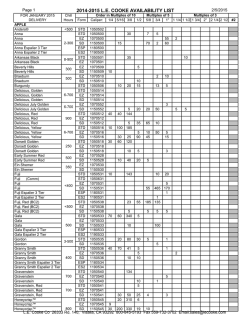

© Copyright 2026