1. Art and Diseño

Density-functional theory for classical fluids and solids
C. Ebner
Department of Physics, Ohio State University, Columbus, Ohio 43210
H. R. Krishnamurthy and Rahul Pandit
Department of Physics, Indian Institute of Science, Bangalore 560012, India
We formulate a density-functional theory that is capable of describing simultaneously the solid,
liquid, and gas phases of a simple classical material. The formalism can be reduced to the EbnerSaam-Stroud theory for the liquid-gas case and to a generalized version of the RamakrishnanYoussouff theory for the liquid-solid case. The theory requires as input the direct correlation functions of a uniform fluid. As an example we apply the formalism to the calculation of the phase diagram of a system with Lennard-Jones intermolecular interactions. We obtain the correlation functions from a closure scheme proposed by Zerah and Hansen [J. Chem. Phys. 84, 2336 (1986)]. The
calculated density-temperature phase diagram compares favorably with those obtained from numerical simulations of the same model system. We also compute the equations of state in the solid and
fluid phases.
I. INTRODUCTION
There have been many studies of the condensation of a
gas into a liquid and the freezing of a liquid into a solid
within the framework of density-functional theory.' The
freezing transition in particular has presented a serious
test of the formalisms. An early formulation, by Ramakrishnan and Youssouff, 2 ' 3 and one on which much later
work has been based,1'4'5 expands the liquid-solid freeenergy difference to second order in powers of the density
difference p s ( r ) — pf, ps is the density of the solid and pt is
that of the coexisting liquid. This theory gives reasonable
results for a model hard-sphere system but fails to produce crystallization of systems of particles interacting
with softer cores.6 8 This failure can be overcome by
keeping higher-order terms in the expansion.6'7 For the
particular case of a Lennard-Jones (LJ) potential, the
theory produces crystallization, but the liquid and solid
densities and the pressure at the phase transition are
rather high,9 a shortcoming which, again, is partially
remedied by including some third-order terms in the expansion. '
However, the inclusion of higher-order
terms when treating hard spheres actually gives rise to inferior results in comparison with those from the secondorder expansion.12 Hence there are basic questions as to
the accuracy and predictive power of the functionals employed in each of these calculations.
A somewhat different approach to constructing a density functional, pioneered by Tarazona13 and others, 14 ~ 20
is to express the solid's free energy as that of a fluid at
some "effective" density. Various of these theories have
produced quite good results in certain applications. For
example, Curtin and Ashcroft21 obtained a quantitatively
correct phase diagram, in comparison with Monte Carlo
simulations, for a LJ system using the weighted-density
approximation14 (WDA) to calculate the properties of a
hard-sphere system and then doing a perturbation expansion around this system. And de Kuijper et al.9 had
similar success for the freezing of a LJ system using the
modified weighted-density approximation20 (MWDA),
provided they treated the attractive part of the interaction via mean-field theory. However, when they applied
the MWDA to the full LJ potential, there was no freezing
transition at all at temperatures below about four times
the critical temperature. See Ref. 9 for a more complete
description of these and other interesting results from attempts to apply various density functionals to the freezing of simple systems.
In this paper we develop a density-functional formalism which has the useful qualities that it is relatively easy
to motivate and simple to apply, with no input other than
the two-particle direct correlation functions of the uniform fluid. Moreover, it can be used in situations where
all three phases—gas, solid, and liquid—of a simple system are present and has the appealing property that for
the gas-liquid subsystem it can be reduced to the densityfunctional theory of Ebner, Saam, and Stroud,22 while for
the liquid-solid subsystem it reduces to a generalized version of the density-functional theory of Ramakrishnan
and Yussouff.2 Finally, we apply the functional to the
calculation of the phase diagram and thermodynamics of
a LJ system. The results are qualitatively very good;
quantitatively speaking, they are not fully satisfactory as
regards the liquid-solid transition, although they are generally superior to those obtained from other functionals
that do not make recourse to perturbation or mean-field
treatments of the attractive part of the interaction.9
In Sec. II we develop our density-functional theory.
We also review in this section the scheme of Zerah and
Hansen23 which we employ for obtaining the direct correlation functions of a LJ fluid. Section III describes our
calculations and results for the correlation functions,
thermodynamic functions of the fluid and solid, and
phase diagram. Finally, in Sec. IV we summarize and
conclude with a brief comparison of our results with
those of other density-functional theories.
II. DENSITY-FUNCTIONAL THEORY
AND CLOSURE SCHEME
A. Density-functional theory
We begin by expanding the grand free-energy functional for a nonuniform system in a functional Taylor series
about a reference density p0,
-Po\
X
(1)
3!
where nid is the free energy of the ideal gas, /3 is the inverse temperature, and the C(n} are the n-particle direct
correlation functions. Also,
and so on. Continuing from Eq. (5), we can formally sum
the expansion if we make use of the Fourier transforms of
Eqs. (4), which are
p(r)
Pid
)- Jfl! 3 rp(r) ,
(2)
(7)
3
where // is the chemical potential and pid = A,~ , A, being
the thermal wavelength.
Now, since the free energy must be independent of p0,
we have the condition that
d(/3W) ^
(3)
etc., to obtain
:> (P-pv]n+
-!3co=-l3co0-C(l\p0)(p-p0)n=0
•°
(n+2)!
for any p0. Consequently we find
(P~po)"
(4)
9
U
r ^ ( 2( 2
) ,)
[C
(r-r';p 0 )]= J c^C^W^Spo) ,
(8)
The summation can be done exactly in the form of integrals of the correlation function Cg 2) (p) over the density, leading to
PO
and so on.
Consider first a constant density system, p(r)=p. We
can compute the integrals in Eq. (1) in terms of zerowave-vector Fourier components of the correlation functions
Po
(9)
and the order of integrations can be exchanged to obtain
-fra=
-/?« 0 -C (1) (poHp-po)-J fPdp2(p-p2)C{02>(p2)
(10)
(5)
More generally, we define the Fourier transforms of the
correlation functions by
where we have made use of the fact that
9C (1) (p)/ap = C'|)2); see the second of Eqs. (4). Finally,
Eq. (10) can be simplified to read
PO
(11)
Notice that the condition for equilibrium, dco/dp = 3, implies that the equilibrium density is given by
Xe
(6)
(12)
Now let us choose p0 = 0. Then a}0=0 and C(l\pQ) =
Hence
I3FS
p(r)ln
-pa)=-fPdp}C(l\Pl)
(13)
is our final result for the free energy of a uniform system.
Consider next the case of a uniform solid. Start once
again from Eqs. (1) and (2). Set Po = 0 as before and expand the density in a Fourier series,
,'G-r
(14)
where the G's are reciprocal-lattice vectors. Then the
free energy, Eq. (1), may be written as
p(r)
Pid
2!
G,,G 2
(15)
where v is the volume of a primitive cell of the crystal
and ps is p G =<> the mean density in the solid.
We next collect terms with all G, equal to zero, two G,
not equal to zero, three G, not equal to zero, etc., and use
relations (7) to get
p(r)
Pid
V
C
-/
•* n'
G(PS}PGP-G •
(17)
The superscript (2) has been dropped from the symbol for
the direct correlation function.
Notice that, if we have a uniform system so that p G =0
for G=7^0, Eq. (17) reduces to an appropriate expression
for the Helmholtz free-energy density of that uniform
system, as may be seen by making the appropriate
modification of Eq. (13). It is in fact identical to the expression for the free energy of a uniform fluid given by
Ebner, Saam, and Stroud.22 Further, Eq. (17) is essentially the same as the free-energy functional of Ramakrishnan and Youssouff, except that the uniform reference
density about which it is expanded is the solid density and
not the liquid density which is equivalent to summing exactly all terms in the free energy which are precisely of
second order in po with G^O and summing terms of all
orders in the uniform density change.
Implementation of Eq. (17) involves, first, obtaining
C ( 2 ) for uniform systems and, second, minimization of
the free-energy functional with respect to p(r) at some
fixed value of p s . We have obtained the correlation functions by methods described in Sec. IIB. As for the
minimization, there are two standard procedures. One is
to expand the density as a Fourier series, Eq. (14), and to
minimize with respect to the amplitudes pG for G^O.
The second is to parametrize the density as a periodic
sum of Gaussian functions and to minimize with respect
to appropriate parameters.
We have chosen the second route. The density is written as
3/2
p(r)=psv
3!
.
p(r)
Pid
(16)
In the application that follows, we drop terms involving C ( n > with n =3 or larger and so have a simple
prescription for the grand free energy of the solid in
terms of the direct two-particle correlation function of a
uniform system with the average density of the solid.
Also, in practice we work with the Helmholtz free energy
which can be obtained by adding a term Pnps to the
right-hand side of Eq. (16). Finally, we set the ideal gas
reference density to unity. Hence we have the following
expression for the Helmholtz free-energy density, in units
of / 3 1 , of a solid with density ps:
JL.
2-rr
-r(r-R)V2
(18)
where the vectors R are lattice translations of the assumed crystalline structure (fee). For given ps, we find
the values of the nearest-neighbor distance or lattice constant a and of the parameter y from the condition that
the free energy be minimized. In this way one obtains a
curve of free energy as a function of a. Notice that the
primitive cell volume v depends on a and that in the absence of vacancies, the product psv=b would be unity as
there would be one particle in each primitive cell of
volume v. Typically, the minimum is obtained for a value
of a at which b is a few percent smaller than one (see Sec.
III).
The evaluation of the ideal-gas part of the free energy
involves only an integration over the logarithm of the
density. Because the overlap of the Gaussian functions
on neighboring sites is extremely small for all cases of interest (see Sec. Ill), it can be neglected and the integral
done analytically,
3/2
3/2
In
LIT
V
2-77
3/2
=A0n
V
(19)
JL
2ir
As for the term involving C, it is evaluated as follows.
First,
ians, Eq. (18), we can show that
,
C G p G p_ G =
3/2
, — r ( r + R ) /4
C (p }p2
(20)
Integration is over the (ultimately infinite) volume V of
the system. Expanding the density as a sum of Gauss-
w
F
(21)
/<
4ir
Next, we integrate over the directions of r and express
the result as a sum over shells of atoms in the lattice
structure. After this is done and the pieces of the free energy assembled, we have
3/2
Mm
»| ta
6
~-|
"27T
ft J 0
<*P<P
P
(22)
Rs and Ns are, respectively, the radius of the 5th shell of
atoms and the number of atoms in this shell. From this
point, the integration is completed numerically and the
free energy minimized with respect to b and y.
The free energy of the solid must be compared with
that of a uniform fluid to obtain the equilibrium phase diagram of the system. The corresponding expression for
the free energy of a fluid with density pf is
/3Ff _
-=pfln(pf)-pf+ f
ff
dp(p-pf)C0(p)
.
(23)
B. Closure scheme of Zerah and Hansen
24
Extending the work of Rogers and Young, Zerah and
Hansen23 have proposed a closure scheme which yields
the pair distribution function of a simple classical fluid as
the solution of an integral equation. The essence of this
closure scheme is to interpolate smoothly in real space
between the hypernetted-chain (HNC) closure, which is
known to work well for the long-ranged part of a potential such as the van der Waals potential, and the soft-core
mean-spherical approximation (SMSA), which is known
to work well for potentials with a soft repulsive part and
a small attractive part.
The procedure is as follows. First, the interparticle potential v (r) is divided into two pieces, v =vl+v2 with
v(r)-vm,
v , ( r ) = 0, r>r
m
and
(25)
v ( r ) , r>rn
where vm is the minimum value of the potential, located
at r = rm. Next, the proposed closure relation is
, .
g(r) =
1+-
where g ( r ) is the pair distribution function and
h(r)=g(r)—l is the total correlation function. The
"switching function" a (r) goes to zero at small r and to
unity at large r so that the closure reduces to, respectively, the SMSA closure and the HNC closure in these limits. Following Zerah and Hansen (who in turn follow
Rogers and Young), we shall take the switching function
to be of the form
a(r)=\-e~ar
(27)
with the single parameter a determined by the condition
that the virial and compressibility equations of state are
identical.
Combining Eq. (26) with the Ornstein-Zernike relation,
3
r<rn
(26)
a(r)
h ( r ) = C(r)+pfd r'h(r-T')C(r'),
(24)
and using the Lennard-Jones (6-12) potential,
"
(28)
12
0.6
(29)
we have obtained, except in the region of spinodal
decomposition, fluid pair distribution functions and
direct correlation functions for temperatures and densities of importance for the purposes of calculating the
phase diagram. In the region of unstable fluid, we have
obtained the direct correlation functions by simultaneously interpolating in density between correlation functions in the gas and liquid regions and extrapolating
down in temperature from correlation functions at temperatures above the spinodal line. The procedure is the
one described and used in Ref. 22.
0.4
0.2
0.6
III. CALCULATIONS AND RESULTS
A. Correlation functions
Using Eqs. (26) and (28) with the intermolecular potential (29), we solve for the C ( r ) and g ( r ) at a given density
and temperature on a grid of evenly spaced points in r using an iterative procedure. The spacing of the points is
0.03cr and the functions are determined out to r = 10.5<r.
The iterations are done in one of two ways; the first is to
use as the input for a given iteration a mix of the input
and output of the previous iteration, and the second,
which has been described in detail by Ng,25 is to construct an optimized input for a given iteration by making
use of the input and output from several (typically two to
four) previous iterations. The latter method is more complicated but usually produces much faster convergence.
The criterion for convergence is that, in the final iteration, the input and output for C ( r ) should differ nowhere
by more than 10~6.
The correlation functions have been found for reduced
densities p* =pcr3 up to 1.2 and for reduced temperatures
T*=kT/e between 0.5 and 1.5. Intervals of T* and p*
are usually 0.1 and 0.05, respectively, but smaller intervals are employed in some instances. In the region of spinodal decomposition (within the closure scheme employed) we obtain direct correlation functions from the
interpolation and extrapolation procedure described in
Ref. 22.
Zerah and Hansen23 have discussed the correlation
functions produced by the closure scheme Eq. (26) and
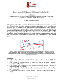
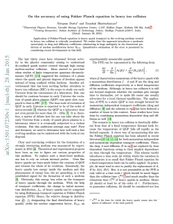
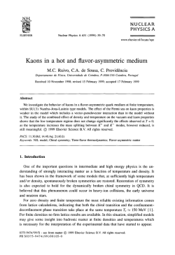
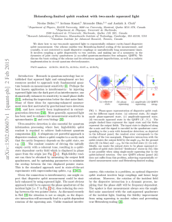
have made detailed comparisons with results of simulations for the same system as that considered here; consequently we shall restrict our discussion to a few representative results. Figure 1 displays the reduced switching
parameter a*=acr as a function of p* (except in the region of spinodal decomposition) at several temperatures;
it is relatively small at large densities and becomes large
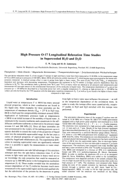
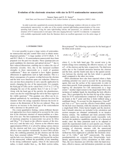
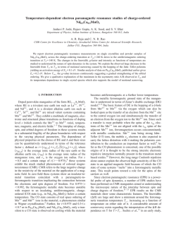
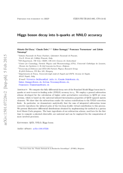
at small densities where the HNC closure, which is obtained in the limit a0—>• oo , is more accurate. In Fig. 2 we
show the structure factor
(30)
at several densities and temperatures close to points of
two- or three-phase coexistence and also close to the criti-
0.8
1.2
1.4
FIG. 1. The reduced switching parameter a* is plotted
against p* at temperatures T*=0.1, 1.0, and 1.3.
cal point. These figures demonstrate the competition of
the peaks at zero wave number and at wave numbers
characterizing the inverse lattice spacing of the solid.
B. Thermodynamics and phase diagram
We have evaluated the Helmholtz free-energy density
/ =F/V, chemical potential (i, and pressure P in the
fluid and solid phases as functions of p* and T*. In the
following, the reduced thermodynamic functions
/*=<7 3 //e, [J.* =n/e, and P*=a 3 P/e are presented. In
the fluid phases the free energy is easily evaluated, given
the direct correlation functions, from Eq. (23); in the
(1.35,0.3).
!>(0.7,0.85)
S(k*)
(1.1,0.05)
-(1.1,0.6)
FIG. 2. The structure factor is shown as a function of
k* = ka/2ir for r* = 1.35, p*=0.30 (
); r* = 1.10,
p*=0.05 (
); r* = 1.10, p*=0.60 (
); and
r*=0.70, p*=0.85 (
). Each curve is labeled with the
corresponding (T*,p*).
solid phase we find /* from Eq. (22) by numerically
evaluating the integrals using Gaussian quadrature and
interpolation of the tabulated correlation functions. It is
necessary to do this many times while minimizing the
free energy with respect to b and y for given p and T.
One hundred shells of lattice sites are retained in the
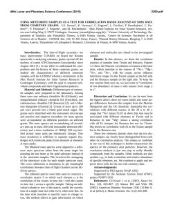
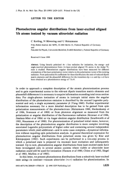
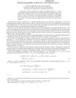
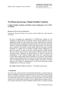
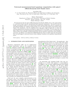
sum. Figure 3 displays 7* = ycr2 for the equilibrium solid
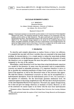
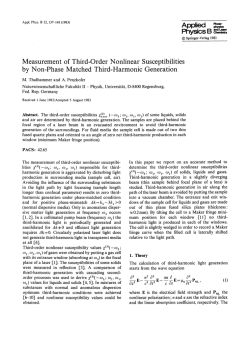
as a function of p* at several temperatures while Fig. 4 is
the analogous plot of b.
Once /* is known, for either type of phase, the chemical potential is found from /x*=3/*/3p*, and then the
pressure (or the grand free energy) follows from
P*=p,*p* —f*. Phase equilibria are determined from
knowledge of/*(p*) for the appropriate phases by making (numerically) a double-tangent construction. Figure 5
shows P*, /j,*, and /* for the fluid phases as functions of
p* at temperatures of (a) 0.7, (b) 1.0, and (c) 1.3. Figure 6
shows the same for the solid phase. From the curves for
/* in Fig. 5 one can make the appropriate double-tangent
construction to obtain the gas-liquid coexistence densities; Fig. 7 is a representative double-tangent construction for liquid-solid coexistence and is at T* = 1.0. Finally, the density-temperature phase diagram is presented in
Fig. 8; Fig. 9 displays more detailed plots of the temperature dependences of the liquid density, the solid density,
and the pressure as functions of the temperature at coexistence. Included for comparison are results from Monte
Carlo simulations26 ~ 28 of the LJ system.
Several remarks are in order. First, the gas-liquid
coexistence curve as determined here is in considerably
better agreement with both Monte Carlo simulations of
the LJ system and with real fluids which the LJ system
approximates, such as argon, than the one found in Ref.
22. Given that the same functional was used to find the
fluid free energy in both calculations, the improvement
must be attributed to the closure scheme employed in
determining the correlation functions. In Ref. 22, the
Percus-Yevick (PY) closure was employed; in the present
work, the closure Eq. (26) proposed by Zerah and Hansen23 has been invoked. The implication is clearly that
the latter is significantly superior. Moreover, the entire
phase diagram compares favorably with results from
simulations of the LJ system, cf. Figs. 8 and 9, especially
given the relatively simple and straightforward density
functional that we employ and the absence of adjustable
parameters. For example, we find a triple-point temperature of T* = 0.665; the experimental value for argon29 is
close to 0.70. It is worth noting in this context that we
also computed the properties of the solid phase and the
solid-liquid phase boundary employing PY correlation
functions. The results for the latter were considerably
less satisfactory than those presented here; for example,
the triple-point temperature was much larger, about 1.1
in reduced units.
IV. SUMMARY
We have constructed a relatively simple densityfunctional formalism for classical systems which allows
for solid, liquid, and gas phases. It extends and consolidates the theories of Ebner, Saam, and Stroud22 for fluid
**/:1000
1.3
0.9
1.0
1.2
FIG. 3. The parameter -y* for the equilibrium solid is shown
as a function of p* for T* =0.7, 1.0, and 1.3.
systems and of Ramakrishnan and YoussoufF2 for solid
systems. The sole input needed for application of the
theory is direct correlation functions of the uniform fluid;
there are no fitting parameters. In the application of the
formalism presented here, we have obtained these correlation functions using a closure scheme proposed by
Zerah and Hansen23 which is demonstrably superior to
other simple approximate closures such as the PY and
HNC approximations.
We have applied the formalism to the calculation of
the phase diagram of a Lennard-Jones system and have
also calculated some thermodynamic properties—free
energy, pressure, and chemical potential—in the fluid
0.96
0.94
b 0.92 -
0.90 -
0.88
FIG. 4. The parameter b for the equilibrium solid is shown as
a function of p* for r* = 0.7, 1.0, and 1.3.
TABLE I. Comparison of freezing parameters at T* — 1 obtained from the Haymet and Oxtoby
(HO) formulation as implemented in Ref. 9, the MWDA + MF of Ref. 9, our calculations (present), and
Monte Carlo (MC) simulations, Refs. 26-28. The quantities presented are the reduced densities p* and
p* of the liquid and solid at coexistence, the relative density change Sp/p; upon freezing, the reduced
pressure P* at freezing, and the Lindemann parameter L. This table is adapted from Table 2 of Ref. 9.
We note that MC simulations were not reported at this temperature in Refs. 26-28; the entries in the
table are obtained by interpolating between results at higher and lower temperatures.
Theory
Pf
P:
Sp/p,
P*
L
HO
MWDA+MF
Present
MC
0.974
0.88
0.944
0.910
1.094
1.025
1.084
1.005
0.12
0.16
0.15
0.10
6.0
3.2
4.8
3.6
0.105
0.100
0.12
0.14
f*, n*, P*
f*, n*, p*
f*, \i», p*
0.0
FIG. 5. The thermodynamic functions P*, /*, and /z* in the fluid phases are shown as functions of p* at temperatures 7"* of (a)
0.7, (b) 1.0, and (c) 1.3.
f*, n*, P*
1.0
p,
1.1
FIG. 6. The thermodynamic functions P*, /*, and (i* in the solid phase are shown as functions of p* at temperatures T* of (a)
0.7, (b) 1.0, and (c) 1.3.
-3.0
0.5
i
-3.4
0.8
I
i
1.0
P*
FIG. 7. The common-tangent construction for the liquid and
solid phases at T* = 1.0; the curves are the reduced Helmholtz
free energies of the liquid and solid phases.
FIG. 8. The calculated density-temperature phase diagram of
the Lennard-Jones system, showing single-phase solid (5), liquid
(L), and gaseous (G) regions and two-phase regions (shaded).
12
1.0
0.9
0.8
0.7
0.9
1.3
FIG. 9. The reduced pressure P", liquid density p f , and solid
density pf at phase coexistence are shown as functions of T*;
results for these quantities from Monte Carlo simulations, Refs.
26—28, are shown as •, •, and A, respectively.
and solid phases. The phase diagram in particular is in
good agreement with experiments on appropriate real
systems, such as argon,29 and with Monte Carlo simulations of the Lennard-Jones system. In Table I we compare freezing parameters determined here with those
from Ref. 4 and from Monte Carlo simulations;26"28 also
included are results from the MWDA + MF scheme of de
Kuijper et al.9
To the best of our knowledge, the only other densityfunctional theory that obtains gas, liquid, and solid
phases and phase boundaries in good agreement with
Monte Carlo simulations is the weighted-density approximation (WDA) of Curtin and Ashcroft.21 (An earlier version of this theory is due to Tarazona. 13 ) Our densityfunctional theory is computationally less taxing than the
WDA; however, it is not straightforward to compare our
theory with the Curtin-Ashcroft implementation of the
WDA for the Lennard-Jones system for the following
reasons: (1) Curtin and Ashcroft obtain their expression
for the free energy of an inhomogeneous liquid by expanding about a reference hard-sphere system which is
treated by using the WDA; it is not clear whether the
WDA would fail for the Lennard-Jones system without
this expansion as a modified version of it (see below) does.
'Density-functional theories of simple classical systems are reviewed by R. Evans, Adv. Phys. 28, 143 (1979); A. D. J. Haymet, Prog. Solid State Chem. 17, 1 (1986); Ann. Rev. Phys.
Chem. 38, 89 (1987); M. Baus, J. Stat. Phys. 48, 1129 (1987).
2
T. V. Ramakrishnan and M. Youssouff, Solid State Commun.
21, 389 (1977).
3
T. V. Ramakrishnan and M. Youssouff, Phys. Rev. B 19, 2775
(1979).
(2) Curtin and Ashcroft use an approximation for determining the direct correlation function which we believe is
not as accurate as the Zerah-Hansen23 closure which we
employ. (3) Lastly they parametrize the Lennard-Jones
potential as a sum of two exponentials. Denton and Ashcroft20 have recently proposed a modified weighteddensity approximation (MWDA) that combines the advantages of the WDA with the computational simplicity
of the original Ramakrishnan-Yussouff 2 densityfunctional theory. However, as de Kuijper et al. have
shown, the MWDA does not yield a solid phase at all, either stable or metastable, at temperatures T* < 5. In order to obtain a solid phase they treat the attractive forces
in a mean-field fashion, leading to the MWDA + MF
scheme, cf. Ref. 9. Further, the modified effective liquid
approximation (MELA) of Baus19 also does not yield a
solid phase in the range of 1 < T* < 10, as pointed out in
Ref. 9. Thus we believe that our density-functional
theory is superior, both qualitatively and quantitatively,
to most other DF theories and that it is comparable to
the best, e.g., the WDA of Curtin and Ashcroft or the
MWDA + MF of de Kuijper et al. Also, it is at the same
time computationally as simple as the original EbnerSaam-Stroud22 and Ramakrishnan-Yussouff2 theories.
In the future we hope to apply the formalism to other,
more complex problems involving nonuniform systems
containing gas, liquid, and solid phases of a simple material; a case in point is the surface-melting30
phenomenon. To study this and similar problems, it will
be necessary to build appropriate nonuniformities into
the parametrization of the density. Preliminary investigations of the surface melting problem in particular indicate that this added complication is well within the capabilities of available computing machinery.
ACKNOWLEDGMENTS
We wish to thank T. V. Ramakrishnan and S. Sengupta
for useful discussions. This work was supported in part
by the University Grants Commission and Department of
Science and Technology (India) and by National Science
Foundation Grant Nos. DMR-8705606 and DMR9014679. Two of us (R.P. and H.R.K.) thank the Ohio
State University Department of Physics for hospitality
while part of this work was being done. The numerical
work was done using the Ohio State University Department of Physics VAX 8650 and the Ohio Supercomputer
Center CRAY Y-MP8/864.
4
A. D. J. Haymet and D. J. Oxtoby, J. Chem. Phys. 74, 2559
(1981).
5
D. J. Oxtoby and A. D. J. Haymet, J. Chem. Phys. 76, 6262
(1982).
6
J.-L. Barrat, Europhys. Lett. 3, 523 (1987).
7
J.-L. Barrat, J.-P. Hansen, G. Pastore, and E. M. Waisman, J.
Chem. Phys. 86, 6360 (1987).
8
M. Rovere and M. P. Tosi, J. Phys. C 18, 3445 (1985).
9
A. de Kuijper, W. L. Vos, J.-L. Barrat, J.-P. Hansen, and J. A.
Schouten (unpublished).
10
C. Marshall, B. B. Laird, and A. J. D. Haymet, Chem. Phys.
Lett. 122, 320 (1985).
"B. B. Laird, J. D. McCoy, and A. D. J. Haymet, J. Chem.
Phys. 87, 5449 (1987).
12
W. A. Curtin, J. Chem. Phys. 88, 7050 (1988).
13
P. Tarazona, Mol. Phys. 52, 81 (1984); Phys. Rev. A 31, 2672
(1985).
14
W. A. Curtin and N. W. Ashcroft, Phys. Rev. A 32, 2909
(1985).
15
M. Baus and J. L. Colot, Mol. Phys. 55, 653 (1985).
16
F. Igloi and J. Hafner, J. Phys. Chem. 19, 5799 (1986).
17
T. F. Meister and D. M. Kroll, Phys. Rev. A 31, 4055 (1985).
18
R. D. Groot and J. P. van der Eerden, Phys. Rev. A 36, 4356
(1987).
19
M. Baus, J. Phys.: Cond. Matter 1, 3131 (1989).
20
A. R. Denton and N. W. Ashcroft, Phys. Rev. A 39, 4701
(1989).
W. A. Curtin and N. W. Ashcroft, Phys. Rev. Lett. 56, 2775
(1986).
22
C. Ebner, W. F. Saam, and D. G. Stroud, Phys. Rev. A 14,
2264(1976).
23
G. Zerah and J.-P. Hansen, J. Chem. Phys. 84, 2336 (1986).
24
F. J. Rogers and D. A. Young, Phys. Rev. A 30, 999 (1984).
25
K.-C. Ng, J. Chem. Phys. 61, 2680 (1974).
26
J.-P. Hansen and L. Verlet, Phys. Rev. 184, 151 (1969).
27
J.-P. Hansen, Phys. Rev. A 2, 221 (1970).
28
J.-P. Hansen and I. R. McDonald, Theory of Simple Liquids
(Academic, New York, 1976).
29
See, e.g., Ref. 28, for summaries of many measured properties
of argon and other rare gases.
30
See, e.g., A. Trayanov and E. Tosatti, Phys. Rev. Lett. 59,
2207 (1987); Phys. Rev. B 38, 6961 (1988), and references
therein.
2I