1. Art and Diseño

NO HYPERBOLIC PANTS FOR THE 4-BODY
PROBLEM
arXiv:1502.00606v1 [math.DS] 2 Feb 2015
CONNOR JACKMAN AND RICHARD MONTGOMERY
Abstract. The N -body problem with a 1/r2 potential has, in
addition to translation and rotational symmetry, an effective scale
symmetry which allows its zero energy flow to be reduced to a
geodesic flow on complex projective N − 2-space, minus a hyperplane arrangement. When N = 3 we get a geodesic flow on the
two-sphere minus three points. If, in addition we assume that the
three masses are equal, then it was proved in [1] that the corresponding metric is hyperbolic: its Gaussian curvature is negative
except at two points. Does the negative curvature property persist
for N = 4, that is, in the equal mass 1/r2 4-body problem? Here
we prove ‘no’ by computing that the corresponding Riemannian
metric in this N = 4 case has positive sectional curvature at some
two-planes. This ‘no’ answer dashes hopes of naively extending
hyperbolicity from N = 3 to N > 3.
1. Introduction
In [1] it was shown that the reduced Jacobi-Maupertuis metric for a
certain three-body problem had negative Gaussian curvature (except at
two points where it is zero). This hyperbolicity led to deep dynamical
consequences. Does hyperbolicity, i.e. curvature negativity, persist
for the analogous N -body problem, N > 3? No. We show that the
analogous reduced 4-body problem with its metric has two-planes at
which the sectional curvature is positive.
The N -body problem in question has equal masses and the inverse
cube law attractive force between bodies.
2. Set-up
Identify the complex number line C with the Euclidean plane R2 .Then
the planar N -body problem has configuration space CN \ ∆. Here ∆ is
the “fat diagonal” consisting of all collisions: ∆ = {q = (q1 , q2 , . . . , qN ) ∈
Date: February 3, 2015.
1
2
CONNOR JACKMAN AND RICHARD MONTGOMERY
CN : qi = qj for some pair i 6= j}. The quotient of CN \ ∆ by translations and rotations is the “reduced N -body configuration space”:
CN = YN × R+ , YN = CPN −2 \ P∆
where CPN −2 is the projectivization of the center of mass subspace
CN −1 = {q ∈ CN : Σmi qi = 0} and P∆ ⊂ CPN −2 is the projectivization
of ∆ ∩ CN −1 . The R+ factor records
the overall scale of the planar N √
gon and is coordinatized by I with I = Σmi |qi |2 being the total
moment of inertia about the center of mass. YN is the moduli space
of oriented similarity classes of non-collision N -gons and will be called
“shape space.”
The following considerations reduce the zero angular momentum,
zero energy N -body problem to a geodesic flow on shape space YN ,
provided the potential V is homogeneous of degree −2. If V is homogeneous of degree −α then the virial identity, also known as the
Lagrange-Jacobi identity, asserts that along solutions of energy H we
have I¨ = 4H − (4 − 2α)V which implies that the only case in which
we can generally guarantee that I¨ = 0 is when α = 2 and H = 0. If
in addition I˙ = 0 then solutions lie on constant levels of I. Now we
recall the Jacobi-Maupertuis [JM] reformulation of mechanics which
asserts that the solutions to Newton’s equations at energy H are, after a time reparameterization, precisely the geodesic equations for the
Jacobi-Maupertuis metric
ds2JM = 2(H − V )ds2
on the Hill region {H − V ≥ 0} ⊂ CN \ ∆ with ds2 the mass metric.
We are interested in the case H = 0, −V > 0 with V homogeneous of
degree −2, in which case the Hill region is all of CN \ ∆ and
ds2JM = U ds2 ,
U = −V
The case of prime interest to us is
(1)
2
U = −V = Σmi mj /rij
where the sum is over all distinct pairs ij. This U , and hence the JM
metric, is invariant under rotations and translations. Quotienting first
by translations we take representatives in the totally geodesic center of
mass zero subspace CN −1 , which reduces the dynamics to geodesics of
the metric ds2JM |CN −1 on CN −1 . Moreover, ds2JM |CN −1 is also invariant
under scaling since the homogeneities of U and the Euclidean mass
metric ds2 on CN −1 cancel. Thus the JM metric admits the group
G = C∗ of rotations and scalings as an isometry group. Now YN is
the quotient space: YN = (CN −1 \ ∆)/G = CPN −2 \∆. (By abuse
of notation, we continue to use the symbol ∆ to denote the image of
NO HYPERBOLIC PANTS FOR THE 4-BODY PROBLEM
3
the collision locus ∆ under projectivization and intersection.) Insisting
that the quotient map π : CN −1 \ ∆ → YN is a Riemannian submersion
induces a metric on YN . Recall that this means that we can define the
metric on YN by isometrically identifying the tangent space to YN at
a point p with the orthogonal complement (relative to ds2JM or ds2 ,
and at any point lying over p in CN −1 ) to the G-orbit that corresponds
to that point. These orthogonality conditions are equivalent to the
conditions that the linear momentum, angular momentum, and ‘scale
momentum’ I˙ are all zero. To summarize, by using the JM metric
and forming the Riemannian quotient, the zero-angular momenetum,
zero energy 1/r2 N -body problem becomes equivalent to the problem
of finding geodesics for the metric defined by Riemannian submersion
on YN .
Remark. The metric quotient procedure just described realizes the
Marsden-Weinstein symplectic reduced space of T ∗ (CN \ ∆) by the
action of translations, rotations and scalings, CoC∗ , at momenta values
0, together with the N -body reduced Hamiltonian flow, but valid only
at zero energy.
Remark This metric on YN can be expressed as U ds2F S where ds2F S
is the usual Fubini-Study metric on CPN −2 .
Remark For the standard 1/r2 potential of (eq. 1) this metric on
YN is complete, infinite volume.
The collinear N -body problem defines a totally geodesic submanifold
RPN −2 \ ∆ ⊂ CPN −2 \ ∆
We obtain this submanifold by placing the N -masses anywhere along
the real axis R ⊂ C, arranged so their center of mass is zero and so
that there are no collisions, and then taking the quotient. In other
words, RPN −2 \ ∆ is the quotient of RN −1 ⊂ CN −1 by dilations and
real reflections.
3. Main result
In case N = 3, with the potential (eq. 1) above, Y3 is a pair of pants
- a sphere minus three points. The point of [1] was to show that the
metric on Y3 just described is hyperbolic provided m1 = m2 = m3 .
Specifically, in this equal mass case the Gaussian curvature of the metric on the surface Y3 is negative everywhere except at two points (these
being the “Lagrange points” corresponding to equilateral triangles.)
What about Y4 ?
Theorem 1. Consider the Jacobi-Maupertuis metric on Y4 induced
as above for the case of 4 equal masses under the strong force 1/r2
4
CONNOR JACKMAN AND RICHARD MONTGOMERY
potential (eq. 1). Then there are two-planes σ tangent to Y4 at which
the Riemannian sectional curvature K(σ) is positive.
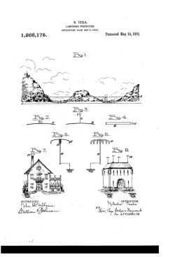
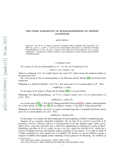
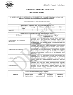
Remark 1. The two-planes σ of the theorem pass through special points p ∈ RP2 ⊂ CP2 which represent certain special collinear
configurations. See figure 1. The two-plane σ at p will be the orthogonal complement to Tp RP2 , the normal 2-plane, and is realized as
σ = iTp RP2 , using the standard complex structure on CP2 .
Remark 2. [Negative curvatures] The RP2 of the previous remark
is a totally geodesic surface fixed by an isometric involution. There are
other such totally geodesic surfaces defined as fixed loci of symmetries,
and computer experiments suggest that these all have negative Gaussian curvature everywhere while their normal 2-planes can have positive
sectional curvature at some points, like our special case RP2 . Computer
experiments also indicate that in the direction of the normal plane there
is positive sectional curvature over all collinear configurations of RP2
and not just the special configurations verified in the theorem. An
analytic proof of these claims beyond our special case however looks
frightening.
Open Question. A geodesic flow can still be hyperbolic as a flow,
without the underlying metric having all sectional curvatures negative.
Is geodesic flow on Y4 hyperbolic as a flow? Is it even partially hyperbolic?
4. Proof of the theorem
We take the case N = 4 in the above considerations. When all
the masses are equal to 1 then the mass metric, used to compute the
kinetic energy and moment of inertia, is the standard Hermitian metric
in coordinate (q1 , q2 , q3 , q4 ) ∈ C4 , where the qi represent the postions
of the ith body. We reduce by translations by going to the centerof-mass-zero space which is a 3-dimensional subspace C3 ⊂ C4 having
Jacobi coordinates as Hermitian orthonormal coordinates :
L
C3 → C4 given by matrix
 1
2
 1
 2

− 1
 2
− 21
√1
2
− √12
0
0
0
0 



√1 
2 
− √12
in standard bases.
As is well-known, if we start tangent to the center-of-mass-zero subspace L(C3 ) we stay tangent to it. Hence we can restrict the dynamics,
potential, metric, etc. to the center-of-mass zero subspace. We denote the potential restricted to the center of mass zero subspace in
NO HYPERBOLIC PANTS FOR THE 4-BODY PROBLEM
5
Jacobi coordinates as UL = U ◦ L and still write ds2JM = UL ds2 for the
restricted JM metric on C3 \∆ where ds2 is the standard metric on C3 .
Continuing along the outline above, we now quotient by scaling and
rotation isometries, C∗ , of ds2JM to obtain the “shape space” Y4 and
we label the quotient map π : C3 \∆ → Y4 which takes a configuration
q to it’s orbit C∗ q. We denote the vertical and horizontal distributions
dπ
as Vp = ker dp π = Cp and Hp = V ⊥ ∼
= Tπ(p) Y4 . Requiring dπ|H,ds2 |
p
JM H
to be an isometry defines our induced metric on Y4 whose geodesics
correspond to N -body motions in “shape space”. Under this induced
metric on Y4 we denote sectional curvature through the plane σ ∈
Tπ(p) Y4 by K(σ).
Suppressing the notation of evaluating at a representative p ∈ π(q),
our main tool in the computation of K(σ), the ds2JM curvature, is the
equation:
(2)
3
U2
UL3 K(σ) = ((∂1 UL )2 +(∂2 UL )2 )−k∇U/2k2 −UL /2(∂12 UL +∂22 UL )+3 L2 (v1 ·iv2 )2
4
kpk
Here ∂a f denotes df (va ) where f ∈ C ∞ (C3 ) and where a = 1, 2
with v1 , v2 ∈ H being ds2 -orthonormal vectors whose pushforwards
dπva span σ. The 0 ·0 , k k, ∇ refer to the norm, metric, and Levi-Civita
connection for the Euclidean metric ds2 . For the derivation of (eq. 2)
see Appendix A.
The collinear configurations form a totally geodesic RP2 ⊂ CP2
which is the image under the projection π of the real 2-sphere in C3
whose points we parameterize as
p = (cos φ cos θ, cos φ sin θ, sin φ).
We evaluate (eq. 2) and find positive sectional curvature over the
configurations with θ = π/2 (see figure 1) in the direction of the iT RP2
plane. This plane is spanned by the pushforwards of
∂p
v1 = −i
= i(sin φ cos θ, sin φ sin θ, − cos φ)
∂φ
i ∂p
= i(− sin θ, cos θ, 0).
cos φ ∂θ
TERMS 1: Over RP2 in the iT RP2 direction, the last term 0 ·0 and
first two terms (the first partials) of (eq. 2) vanish:
v2 =
v1 · iv2 = 0, ∂a UL = 0.
That v1 · iv2 = 0 is clear: i rotates v2 into purely real coordinates. To
evaluate the 1st partials, note Lp has purely real coordinates and ∇U
6
CONNOR JACKMAN AND RICHARD MONTGOMERY
Figure 1. : The collinear configurations p which we consider.
k
, so ∇|Lp U has purely real coordinates.
has kth component j6=k qjr−q
4
jk
Now since Lva has purely complex coordinates,
P
∂a UL = ∇|Lp U · Lva = 0. TERMS 2: With the notation Lp = (q1 , q2 , q3 , q4 ), Lva = i(va1 , va2 , va3 , va4 )
1
and ρjk = qj −q
, αjk = (v1j − v1k )2 + (v2j − v2k )2 ∈ R, the 2nd partials
k
terms of (eq. 2) are:
∂12 UL + ∂22 UL = −2
X
αjk ρ4jk .
j>k
We write our standard coordinates on C4 as qj = xj + iyj , then since
Lva is purely imaginary:
∂a2 UL = ∇|Lp (∇U · Lva ) · Lva = (∇|Lp
Next we compute
so now:
∂a2 UL = −2
X 4
ρ
X 4
∂ 2U
∂ 2U
|Lp = 2ρ4jk for j 6= k and
| = −2
ρjk
2 Lp
∂yj ∂yk
∂yk
j6=k
k 2
j k
jk ((va ) −va va )
j6=k
∂U k
∂ 2U
va ) · Lva =
|Lp vak vaj .
∂yk
∂yj ∂yk
= −2
X 4
ρ
k 2
k j
j 2
jk ((va ) −2va va +(va ) )
= −2
j>k
k
j 2
jk (va −va ) .
j>k
RESULT: Over the circle θ = π/2, K(iT RP2 ) is positive.
For, substituting terms 1 and 2 into formula (eq. 2), we see that:
0 < K ⇐⇒ 0 < UL3 K = −k∇U/2k2 + UL
X 4
ρ
X
j>k
αjk ρ4jk ⇐⇒
NO HYPERBOLIC PANTS FOR THE 4-BODY PROBLEM
X X 3 2
( ρ )
(3)
jk
k
<(
αjk ρ4jk )
jk )(
j>k
X 2
ρ
j>k
j6=k
7
X
Taking θ = π/2 and with the notation introduced in terms 2, we find
the relations:
1
1
, ρ34 = √
2 cos φ
2 sin φ
√
2
=
= −ρ24
cos φ − sin φ
√
2
=
= −ρ23
cos φ + sin φ
ρ12 = √
ρ13
ρ14
1
1
, α34 = 2
2
ρ34
ρ12
1
α13 = 2 + 1 = α24
ρ14
1
α14 = 2 + 1 = α23 .
ρ13
Now the left side of (eq. 3) works out to:
α12 =
2((ρ312 + ρ313 + ρ314 )2 + (ρ313 − ρ314 − ρ334 )2 ) =
= 2(
X 6
ρ
3
3
3
3
3
3
jk +2ρ12 (ρ13 +ρ14 )+2ρ34 (ρ14 −ρ13 )) = 2
k>j
X 6
ρ
jk −96
k>j
=
X 6
2
ρ
jk
1
=
sin 2φ cos2 2φ
2
+ negative term
k>j
and the right side of (eq. 3) works out to:
(ρ212 + ρ234 + 2(ρ213 + ρ214 ))(
=(
ρ412 ρ434
ρ413 ρ414
4
4
+
+
2(ρ
+
ρ
+
+
)) =
13
14
ρ234 ρ212
ρ214 ρ213
cos2 2φ 6
2
8
2
6
6
+
)(sin
2φ(ρ
+ρ
)+
(ρ13 +ρ614 )+2(ρ413 +ρ414 ) =
12
34
2
2
2
sin 2φ cos 2φ
=2
X 6
ρ
2
jk +cot
k>j
2φ(ρ613 +ρ614 )+8 tan2 2φ(ρ612 +ρ634 )+(ρ413 +ρ414 )(
4
16
+ 2 )=
2
sin 2φ cos 2φ
8
CONNOR JACKMAN AND RICHARD MONTGOMERY
=2
X 6
ρ
jk
+ positive term.
k>j
Therefore the inequality (eq. 3) holds!
5. Acknowledgment.
We would like to thank Slobodan Simic [San Jose State, San Jose
,CA] for discussions on hyperbolicity, and Prof. Jie Qing [UCSC]
and Wei Yuan of UCSC for conversations regarding curvature computations. We thankfully acknowledge support by NSF grant DMS20030177.
Appendix A. DERIVATION OF eq. 2:
Take a ds2 -orthonormal basis {va } for C3 with v1 , v2 ∈ Hp .
The Kulkarni-Nomizu [K-N] product formula for conformal curvatures ([3], pg. 51) reads:
1
¯ abcd − UL Rabcd = −{ds2JM ○(∇du
∧
R
− du ⊗ du + kduk2 ds2 )}abcd
2
where u := 21 log UL and the overbars denote curvature with respect to
the ds2JM -metric and all other quantities (no overbars) are with respect
to the ds2 -metric. Then Rabcd = 0 since ds2 is the flat Euclidean metric
of C3 = R6 . Taking cd = ab we have:
¯ ab = R
¯ abab = −UL (∇dubb +∇duaa −dub ⊗dub −dua ⊗dua +kduk2 ) =
UL2 K
= −UL (∂a2 u + ∂b2 u − (∂a u)2 − (∂b u)2 + k∇uk2 ).
Next O’Neill’s formula ([2], pg. 213) gives
¯ 12 + 3 |[V1 , V2 ]V |2 2
K(dπv1 , dπv2 ) = K
dsJM
4
where Va = √ va and X V denotes ds2JM projection of X onto V.
UL (p)
We then compute:
∂a u =
∂a UL
∇|Lp U · Lva
=
2UL
2UL (p)
and
∂a2 u =
∂a2 UL (∂a UL )2
∇|Lp (∇U · Lva ) · Lva (∂a UL )2
−
=
−
.
2UL
2UL2
2UL (p)
2UL (p)2
NO HYPERBOLIC PANTS FOR THE 4-BODY PROBLEM
9
Note that ∇U ∈ {q ∈ C4 : qj = 0} and Lva is a ds2 orthonormal
basis for this center of mass zero subspace, hence
P
k∇U k2 =
X
(∇U · Lva )2 =
(∂a UL )2 = 4UL2 k∇uk2 .
X
Substitution into the K-N formula gives
¯ 12 = − 1 ( UL (∂12 UL + ∂22 UL ) − 3 (∂1 UL2 + ∂2 UL2 ) + k∇U/2k2 ).
(4) K
UL3 2
4
To compute O’Neill’s Lie bracket term we write our standard coordinates on C3 as (x1 + ix2 , ..., x5 + ix6 ).
Let H1 = X j ∂xj , H2 = Y j ∂xj ∈ H be any horizontal vector fields.
The vertical vector fields are spanned by the Euler vector field E =
xj ∂xj and iE. Then Hj · E = Hj · iE = 0 and:
[H1 , H2 ] · E =
X
X j xk ∂xj Y k − Y j xk ∂xj X k =
k
=
X
X j (∂xj (xk Y k )−δjk Y k )−Y j (∂xj (xk X k )−δjk X k ) =
k
X
X k Y k −Y k X k = 0
k
and likewise:
[H1 , H2 ]·iE =
(Y j ∂xj X k −X j ∂xj Y k )xk+1 +(X j ∂xj Y k+1 −Y j ∂xj X k+1 )xk =
X
k odd
=2
X
−X k Y k+1 + X k+1 Y k = 2H1 · iH2 .
k odd
Then
|[V1 , V2 ]Vp |2 = ds2JM ([V1 , V2 ],
=
Ep
»
|p| UL (p)
)2 +ds2JM ([V1 , V2 ],
iEp
»
|p| UL (p)
)2 =
UL2
4UL (p)(V1 · iV2 )2
4
2
2
(([V
,
V
]·E)
+([V
,
V
]·iE)
)
=
=
(v1 ·iv2 )2 .
1
2
1
2
2
2
|p| UL
|p|
UL (p)|p|2
Now substitution of this Lie bracket expression and (eq. 4) into
O’Neill’s formula and multiplying by UL3 yields (eq. 2). References
[1] R. Montgomery, Hyperbolic Pants fit a three-body problem, Erg. Th. and Dyn.
Systems, v. 25, (2005), 921-947.
[2] B. O’Neill, Semi-Riemannian Geometry With Applications to Relativity, 1st
ed. 1983, Academic Press.
[3] T. Sakai, Riemannian Geometry, 1st ed. 1992, transl by T. Sakai, Shokabo
Publishing.
10
CONNOR JACKMAN AND RICHARD MONTGOMERY
(Jackman) Mathematics Department, University of California, 4111
McHenry Santa Cruz, CA 95064, USA
E-mail address: [email protected]
(Montgomery) Mathematics Department, University of California, 4111
McHenry Santa Cruz, CA 95064, USA
E-mail address: [email protected]