1. Ingeniería

or PIIYSICS157.
.\NNAI.S
255-281
( 1984)
Surface
H.
the
The response
of a semi-Infinite
random
phase
approximation.
Response
ESBENSEN
of Fermi
AND
G. F.
self-bound
Fermi
liquid
with specific
application
Liquids
BERTSCH
to a surface
field is calculated
using
to the nuclear
surface.
A separable
approximation
for the induced
field is found
to be quite accurate.
There
isoscalar
response
at 7ero frequency
associated
with
the translational
system.
but quantities
such as the energy-weighted
strength.
the surface
is a divergence
degeneracy
tension.
and
in the
of the
the zero
point
fluctuation
of the surface
density
are well behaved.
The theory
is applied
to the inelastic
scattering
of protons
from nuclei.
and it is found
that the nuclear
response
is well reproduced
by the semi-infinite
theory.
( 19X-l Acadcmlc Preai. Inc.
1. INTRODUCTION
The Random Phase Approximation
(RPA) is a remarkably accurate theory of the
response of systems of interacting fermions. For translationally invariant syst$ms, the
long-wavelength
limit provides the Landau theory of Fermi liquids, a useful theory
for the bulk properties of nuclear matter, liquid ‘He, and electrons in simple metals.
In a spherical representation. the RPA provides a description of nuclear excitation
properties, which is useful even for detailed spectroscopy of excited states.
In this work we consider another limit of RPA, the theory of the surface response
of semi-infinite systems. Many physical probes emphasize the surface response of the
medium. For example, the scattering of hadrons from nuclei probes a region of the
nuclear surface whose depth is of the order of the surface thickness. In low-energy
electron scattering from metals, the surface modes play an important role.
The RPA theory of semi-infinite Fermi systems has been developed for electrons in
metals ( I-3 1 and also investigated for the nuclear surface [4 1. However, there are
numerous questions about the surface response that have not been properly
addressed. particularly for self-bound Fermi systems such as nuclei. Some questions
we will try to answer include:
(I)
Are there new features in the surface response qualitatively
the bulk response?
(2) How accurate are simplified
characterizing the surface response?
different from
models, such as the Thomas-Fermi
model, for
255
0003.4916/84
Cupyrtpht
C IYtX
AH rights of reproduction
$7.50
by Academic
Press. Inc.
in any form reserved.
256
(3)
theory?
ESBENSEN
Is the empirically
measured
AND
BERTSCH
response
adequately
described
by the RPA
Before we can address these questions, we need to establish an RPA formalism,
which is done in the next section. By making simplifying assumptions about the
interactions,
we can construct
a solvable model for the surface response. The
simplified model is compared with numerical solutions of the integral equation in
Section 3.
We shall find that self-bound Fermi systems do indeed exhibit surface response
features that are different from the bulk behavior. In other aspects, the surface
response is close to the bulk response at an appropriate density. The comparison to
the Thomas-Fermi
and other simple treatments is made in Section 4. In Section 5 an
effective surface tension is extracted from the static surface polarization. Finally, in
Section 6 we compare the RPA with some empirical energy-loss
scattering
measurements, finding good agreement.
2. THE SLAB MODEL
We begin with a model of the ground state of a semi-infinite slab. The
wavefunction is a product of independent particle wavefunctions, chosen as
eigenstates of a single-particle Hamiltonian. The medium occupies the z < 0 halfspace with the surface in the x --)I plane. The single particle wavefunctions will be
plane waves in the x - y directions, and have a z-dependence which must be
calculated numerically from the Hamiltonian
H, = -g
v2 + V(z).
P-1)
We shall not go through the Hartree-Fock procedure to determine the singleparticle potential V(z) from the interaction via the self-consistent equations. Rather,
we will choose V(z) in a phenomenological way as a Fermi function
V(z) = V,(l + exp(-z/a)>-‘,
and use the self-consistency of the Hartree-Fock to constrain the interaction in the
RPA equation.
2.1. The RPA Equation
For purposes of establishing notation, we shall remind the reader of the RPA
theory. The collective responseis conveniently formulated as an integral equation for
the induced density 8~. The source term is an external perturbation U(r) cos(wt) that
SURFACE
RESPONSE
OF
FERMI
LIQUIDS
257
is periodic in time. Through the residual interaction 7 the induced density generates
the induced potential
6V(r, w) = 1.dr’ 7 ‘(r, r’) dp(r’, to).
(2.3)
The self-consistent induced density is thus determined by
6p(r, co) = - 1.dr’ G,( r, r’, w) (U(r’) + 6V(r’, o)},
(2.4)
where G, is the field-free Green’s function, obtained from first-order perturbation
theory. The construction of G, and the single-particle density p,,(z) in the noninteracting ground state for slab geometry is described in Appendix A. The formal
solution is expressed by the RPA Green’s function
dp=--G,,,
U=-(1
-tG,?“)~‘G,U.
(2.5)
Various approximations for the residual interactions are discussedin Section 2.4.
We shall always assume that they are translationally invariant in the coordinates
measured along the surface of the slab. All Green’s functions are then also trans
lationally invariant in these directions, and it is convenient to introduce their Fourier
representation
G(r, r’, w) = (271)’ [ d2K G(z, z’, K,
OJ)
exp(iK(r, - r;)).
(2.6)
Here rp abd r; are coordinate vectors parallel to the surface, and K is the associated
Fourier vector. The Green’s functions G(z, z’, K, CO)are independent of the orientation of K(cf. Appendix A).
2.2. ResporiseFunctiorts
We next must specify the form of the external field U. This will depend on the
characteristics of the external probe, in particular how strongly the probe is absorbed
by scattering processes.For discussingthe general features of the responseit is useful
to define a particular external field. proportional to the derivative of the singleparticle potential
U(r) = -V’(z)
exp(rKr,).
(2.7)
The responseof the system is then a function of two parameters, viz., the momentum
transfer hK along the surface and the excitation energy hw. Note that K plays a
similar role as the multipolarity does for spherical nuclei. The response function is
defined as
S(K, w) = i
Im I.
/-) dz.1 dz’ V’(z) G(z, z’, K, to) V’(z’)( .
(2.8)
258
ESBENSEN
AND
BERTSCH
The response function is determined by excitations of the system that are on the
energy-shell. The off-energy-shell
transitions are contained in the real part of the
Green’s function, and they are associated with polarizations of the system. To make
this distinction between the response and polarizations
quite clear we define the
dynamic polarization function as follows:
~dz~~dr’V’(z)G(z.z’.K.w)Y’(z~)(.
”
.
(2.9)
Various sum rules for the response are given in Section 2.5.
2.3. RPA for Separable Interactions
in
For a general residual interaction 7. the inversion of the matrix 1 + G,7
Eq. (2.5) is complicated by the fact that perturbations induced by the external field
will propagate into the interior of the slab. and bulk oscillations of the induced
density can again affect the collective surface response through a strong residual
interaction. Using a separable residual interaction, however, one can easily obtain the
we choose the separable
RPA response from the free response. For simplicity
interaction
7 ‘(r* r’) = Ice V’(z)
V’(z’)
(2.10)
g(r, - r;),
where the function g describesthe interaction in directions parallel to the surface, and
the coupling strength K~ can be adjusted in order to simulate more realistic
interactions as discussed in the next section. In the Fourier representation for slab
geometry this interaction becomes
(2.11)
7 ‘(z, z’. K) = K(K) V’(z) V’(z’),
where the K-dependent coupling strength is K(K) = K,~(K),
and we normalize
g(K = 0) = 1. The RPA Green’s function can then be obtained from the expansion
G RPA=GO-G07‘GO+G07‘G07’GO-...
=
G,
-
K(G,,
V’)(V’G,)
(1 +
K(~“G,
V’)}
‘.
(2.12)
The induced density of the collective response can be obtained from the field-free
induced density dp, by
6pRpA(z,K, 0) = &+,(z, K, w)( 1 + K( f”G,(K.
w) V’)} - ‘.
(2.13)
The RPA response can be expressed in terms of the field-free response S, and the
field-free polarization function P, as follows:
S,,,(K.
0) = S,(K, w){ (1 + KP,(K, CO))’+ (KTS,(K, CO))’I -‘.
(2.14)
The RPA response for separable interactions is completely determined by the
SURFACE
RESPONSE
OF FERMI
LIQUIDS
259
coupling constant K and the free response. since the polarization function can be
obtained from the response function through the Kramers-Kronig
relation (2.26).
2.4. Residual Itlteractions
We determine the isoscalar coupling strength K~ from the requirement that an
induced density of the form 6p(z) = -pi(z) 6~ leads to a similar induced potential
6V(z) = -V’(Z) & through the residual interaction. This condition would follow
automatically from a self-consistent Hartree-Fock
calculation. The self-consistency
requirement applied to Eqs. (2.3) and (2.11) yields
h-0’ = j dz&,(z)
V’(z) = - ) dzp,,(z)
v”(z),
(2.15)
which implies that the isoscalar response diverges in the static limit for k’ = 0. TO
demonstrate this point we note that a static displacement of the single-particle
potential leads to the same displacement of the slab density. In first-order perturbation theory one finds in particular (cf. Appendix C, Eq. (C.6))
&+,(z, K = 0. w = 0) = 1 dz’ G,(z, z’, 0, 0) V’(z’) = -p;,(z).
(2.16)
The associated value of the field-free polarization function is
P,(K = 0. w = 0) = - 1.dz V’(z)&(z)
= 1.dz p,(z) V”(z).
(2.17)
The first term in the denominator of (2.14) then vanishes in the static limit.
Moreover, the free responsevanishes linearly in o in this limit as we shall see, and it
follows that the RPA response will diverge as l/w for w -+ 0. A similar result is
found for spherical nuclei, where the spurious isoscalar dipole mode is located at zero
excitation energy. For non-zero values of K the isoscalar response is more well
behaved with a vanishing responseat w = 0.
More realistic interactions, for example, the Skyrme-type commonly used in
Hartree-Fock calculations, have zero range and contain a density dependence. We
shall therefore also study the responseusing interactions of the form
7 ‘(r, r’ ) = L!,(Z) 6’“’ (r - r’ ).
(2.18)
The position dependence is ascribed to a density dependence in the effective
interaction that could be calculated in Brueckner Hartree-Fock theory. Because of
the zero range in (2.18), the function L,<(Z)in the isoscalar channel is determined by
the self-consistency condition to be
u,(z) = V’(z)/Lqz).
260
ESBENSEN
AND
BERTSCH
In the surface region a good fit is given by the function
vc(z) = -50 - 500/( 1 + exp(-z(fm)/0.5))
MeV fm”.
(2.19)
Notice that the interaction is very attractive in the far surface, and that it practically
vanishes in the interior.
For most of our calculations we assume that the interaction has zero range in
directions parallel to the surface. The coupling constant K(K) for the separable
interaction (2.11) is then independent of K. For the isoscalar mode we shall also
study the effect of a finite range. Using a Yukawa interaction of range a,, the Kdependence of the coupling constant is
K(K) = q,( 1 + (Ku,)‘}
(2.20)
-I”,
where K,, is determined by Eq. (2.15).
No self-consistency
argument can be used to determine the interactions for the
isovector and the spin modes. We adopt again the parametrization
(2.18) for each of
these interactions, but ignore a position dependence of vC, which seems reasonable
from empirical studies of the response of finite nuclei. The coupling strength of the
corresponding separable interaction is set by demanding that it has the same diagonal
matrix elements as the microscopic interaction. This leads to the value
--I
K =
21,
I_ dz
i.
(v’(z))2
.
(2.2 1)
i
Numerical
studies of the Gamow-Teller
response
[5 ] show that existing
experimental
data are well
reproduced
using the interaction
(2.18)
with
~1,= 220 MeV fm3 for the (T= 1. S = 1) channel. Similar studies of the isobaric
analog state and the giant dipole resonance (61 indicate that the isovector channel
can be described by the interaction (2.18) with v, = 300 MeV fm3. The residual
interaction in the (T= 0, S = 1) channel is much weaker than in the (T = 1, S = 0)
channel. We adopt the numerical value 2), = 50 MeV fm3 in Section 6.
2.5. Sum Rules
It is useful to define a new response function, the direct response, for our
discussion of the sum rules. Similar to Eq. (2.8) we define the direct response
Sf(K,w)=bIm
/[dzidr’
V’(z)Gg(r,z’.K,w)V’(z’)/,
(2.22)
where the direct field-free Green’s function Gf is defined in Appendix A, Eq. (A.9).
This response does not respect the Pauli principle, and it is non-zero for all transitions down to minus the Fermi energy. The free response, obtained from the
SURFACE
RESPONSE
retarded field-free Green’s function
as follows:
OF FERMI
261
LIQUIDS
(A.6). can be constructed
from the direct response
S”(K, w) = Lq(K. 0) - Sfj)(K, -w).
(2.23)
The second term cancels all forbidden transitions contained in the direct response, so
that the Pauli principle is obeyed. This response is an odd function of w. and all poles
in the complex w-plane are below the real axis, characteristic for a retarded response.
For the particular type of residual interactions considered in the previous section that
all commute with the external field (2.7), one finds [7] that the energy-weighted sum
rule (EWSR) for the RPA response is identical to the EWSR of the free response,
and it is given by
A21.1diuwS(K.w)-~~j~dzpo(z)i(v”(r))2
+K2(V’(z)J2}.
(2.24)
'0
The direct response function
has the normalization
(2.25)
There is no analogous simple sum rule for the total RPA or for the total free
response, integrated over all positive excitation energies. The total free response is
reduced compared to (2.25) due to the Pauli blocking, and the total RPA response
depends strongly on the type of residual interaction being used.
Another important sum rule gives the connection between the response function
and the dynamic polarization function (2.9). This is the Kramers-Kronig
relation.
which states that
The second factor in the integrand is the principal value of l/(w’ - ~0). All the poles
of a retarded response are below the real axis in the complex w-plane. so we can
close the tu’-integration
by a semicircle in the upper complex plane. The only pole
inside this integration path is CCI’= CL)+ it/. and the result (2.26) follows directly. We
shall later use this relation to obtain analytic approximations
for the collective
response. In particular, for K = 0 we obtain the closed expression
I=’ dw ;
-‘La
from the static polarization
S,(K = 0, w) = (_dz p,(z) V”(z)
(2.17) of the non-interacting
ground state.
(2.27)
262
ESBENSEN AND BERTSCH
3. RESULTS OF NUMERICAL
CALCULATIONS
In this section we study the response of a semi-infinite slab as a function of the
excitation energy hw and the momentum transfer hK along the surface. The external
field U is given in Eq. (2.7). To give this field the dimension of energy we shall
always multiply it by 1 fm in displaying our results. We use the parameters
Y0 = 45 MeV and a = 0.75 fm for the single-particle potential (2.2) in order to
simulate the surface properties of heavy nuclei. The field-free Green’s function given
in Appendix A is calculated on a grid with a step size of 0.25 to 0.5 fm. The
integration over the Fermi sphere is performed with a step size of 0.01 to 0.05 fm ’
in the z-direction perpendicular to the surface and in the x-direction parallel to the
momentum transfer hK, whereas the integration over the remaining surface direction
is trivial.
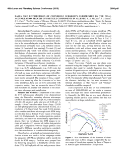
3.1. Resultsfor K = 0
We consider first the collective response (2.14) for separable residual interactions
in the limit K = 0. The coupling strengths for the isoscalar and isovector interactions
are given in Eqs. (2.15) and (2.21), respectively, and the results are shown in Fig. 1,
together with the free response.
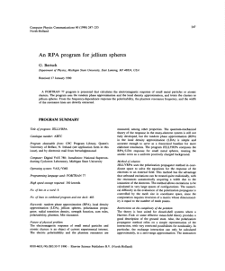
The isoscalar response is seen to be enhanced for hcc,< 10 MeV compared to the
free response. In this region it exhausts about 25% of the energy-weighted sum rule
(EWSR), whereasthe free responseonly contains 7.5% of the EWSR in this interval.
Moreover, it diverges as l/w for o + 0, since we have adjusted the coupling strength
from self-consistency.
The isovector response, on the other hand, is enhanced for large and reduced for
small excitation energiescompared to the free response.Thus the maximum occurs at
an excitation energy 8 MeV higher than that in the free response. For all three
IO
FIG. 1.
transfer
residual
20
%w(MeV)
30
40
Response functions
for the semi-infinite
slab due to the external
parallel to the surface is zero. The collective
response functions
interactions
given in Section 2.4.
50
field (2.7). The momentum
are based on the separable
SURFACE
RESPONSE
OF FERMI
263
LIQUIDS
response functions shown in Fig. 1 the EWSR is the same and it is given
by
Eq. (2.24).
The numerical calculation of the collective response, using the zero-range residual
interactions
(2.18). is more difficult, since the calculation of the RPA Green’s
function (2.5) involves a non-trivial
inversion of the operator
1 + G,?’ ‘. The
inversion can be performed conveniently in coordinate space for spherical nuclei 17I.
For slab geometry one finds that the induced density of the free response is so large
in the interior of the slab that the associated induced potential becomes significant
deep inside the slab surface. One would therefore need a very large interval in coordinate space to obtain reliable numerical results. To overcome this problem we used a
finite damping of d = 2 MeV in the field-free Green’s function. and it was then
sufficient to perform the numerical calculation on a finite interval that reaches
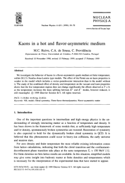
20-40 fm inside the slab surface. The results for the isoscalar and isovector responses
are shown in Fig. 2, together with the response functions for separable interactions,
all obtained with the damping width mentioned above. The two types of interactions
are seen to yield quite similar responses.
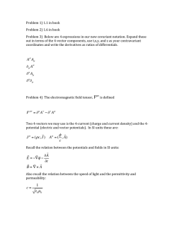
To illustrate in more detail the effect of the zero-range residual interactions (2.18)
we show in Fig. 3 the associated induced densities at an excitation energy of 15 MeV.
For the isovector mode we see that the period of the interior oscillations is much
larger and that the surface peak is much more smeared out than in the case of the
free response, whereas the oscillations
in the isoscalar density have shorter
wavelengths and are enhanced near the surface. This is just the behavior one expects
for the response of an infinite gas. The induced densities for the separable
interactions, which are not shown, deviate from the density of the free response
mainly in the magnitude of the amplitudes. The periods of the interior oscillations are
about the same as for the free response.
ISOSCALAR
o-04-
iFF
\
10
;
20
30
40
50
FIG. 2.
Response
functions
for the semi-infinite
slab obtained
with a finite damping
width of
J = 2 MeV in the field-free
Green’s function.
The free response and the isoscalar and isovector
response
for separable residual interactions
are shown as solid curves. Also shown is the isoscalar
(0) and the
isovector
(A) response for the &function
interactions
discussed in Section 2.4.
264
ESBENSEN
4-
AND
BERTSCH
,
FREE
.
::
, ’
RESPONSE
2-
5
ISOVECTOR
-21
-40
-30
-20
-10
0
’
FIG. 3. Induced densities
associated
with the free response and with the isoscalar
and isovector
response for b-function
interactions.
at an excitation
energy of 15 MeV. The solid curves represent the
real part and the dashed curves are the imaginary
part of the induced densities. The damping width in
field-free Green’s function was d = 2 MeV.
3.2. Lorentzian
Approximation
The free response discussed in the previous section is quite accurately
by a Lorentzian distribution of the form
S,,W, WI= N &
I((0 - ,o12 + (Y/2)2)-’
We can insert this expression
approximation
represented
- (@ + QJo12+ (Y/2)*)-‘}*
into the Kramers-Kronig
(3.1)
relation (2.26) and obtain the
coo-w
wo + OJ
P,(K, w) = N
zt 1 (w - coo>2+ (y/2)2 + (w + wo)2 + (y/2)2 !
(3.2)
for the field-free polarization
function. The RPA response (2.14) for separable
interactions is now also completely determined by these two analytic expressions, and
using the parameters N = 23.0, hw, = 9.4 MeV, and hy/2 = 13.6 MeV, all three
response functions shown in Fig. 1 are quite well reproduced.
SURFACE
3.3. K-Dependent
RESPONSE
OF
FERMI
265
LIQUIDS
Response
We shall now examine the RPA response for non-zero momentum transfers along
the surface. This is illustrated in Fig. 4 by contour plots. The results were obtained
with a vanishing damping width d in the field-free Green’s function and using
separable residual interactions for the collective response. For the isoscalar mode we
included the effect of a finite range Yukawa interaction via the K-dependent coupling
constant (2.20). We used a realistic value of 1 fm for the range of this interaction.
A number of qualitative features of the response functions shown in Fig. 4 may be
noted. First the divergence of the isoscalar response is quite weak. disappearing when
K # 0. For a fixed value of K the response has a peak whose position increases with
increasing K. This is what one would expect from the infinite Fermi gas model. The
peak of the isoscalar response occurs at lower excitation energies than in the free
response, whereas the peak of the isovector response is pushed towards higher
excitations.
The main behavior of the free response shown in Fig. 4 can be reproduced by the
Lorentzian approximation (3.1) using the K-dependent parameters
h,(K)
;
=
9.4 + 0.64 e
MeV,
fi’K2
MeV,
by(K) = 13.6 + 0.93 2m
N(K)=&(K)
1.69 (1 -0.176
(3.3)
K’}
This parametrization
of the free response can also be used to determine the RPA
response (2.14) for separable interactions, as discussed in the previous section. The
result obtained in this way for the isoscalar response is also shown in Fig. 4 and
compares quite well with the numerical calculation.
The effects of Pauli blocking and residual interactions are illustrated in Fig. 5.
where we show the K-dependence of the total response, integrated over all excitation
energies. It has been normalized to the direct sum (2.25). obtained from the direct
response (2.22), which contains all transitions including those that are forbidden by
the Pauli principle. The Pauli blocking is seen to reduce the total free response
considerably for small values of K. We show two results for the isoscalar response,
one with a zero-range interaction along the surface, and one with the finite range of
1 fm. The range of the interaction is seen to have a very significant effect on the total
isoscalar response. The total response is divergent for K = 0 in both cases. It is
always enhanced compared to the total free response, whereas the total isovector
response is reduced. For large values of K the effects of Pauli blocking and residual
interactions are seen to diminish.
The enhancement of the total collective response over the total free response has
been related to a modification
of the ground state density due to the residual
266
ESBENSEN
AND
BERTSCH
I.
",
0
N
x2
I.
0
20
40
60
00
100
20
40
fw(MeV)
60
00
IO
fiw(MeV)
Frc. 4. Contour
plots of the free response and the isoscalar
and isovector
response for separable
interactions.
as functions
of the excitation
energy and the momentum
transfer hK parallel to the surface
of the semi-infinite
slab. For the isoscalar response the coupling
strength (2.20) for a finite range of I fm
was used. Also shown is the isoscalar response obtained,
as described in Section 3.2, from a Lorentzian
fit to the free response with the parameters
given in Eq. (3.3).
1.5
tI
I
ISOSCALAR
1
I
(ZERO-RANGE)
I
I
2
3
4
K2 (fH2)
Ftc. 5. Total responses obtained from the response functions
shown in Fig. 4 by integration
over all
excitation
energies. They are shown as functions of the momentum
transfer hK parallel to the surface of
the semi-infinite
slab and have been normalized
to the total direct response (2.25).
For the isoscalar
response the results for the zero-range
separable interaction
is also shown (dashed curve).
SURFACE RESPONSE OF FERMI LIQUIDS
267
interactions 181. We shall here adopt a similar model and give the final results for
slab geometry without performing a detailed derivation. The particle density in the
interacting ground state p,(z) is related to the Hartree-Fock ground state density
P,,(Z) by the Gaussian folding
/l,(i)
= (27ZAl7’)-“’
(3.4)
cf. Ref. 181. This result is based on a harmonic approximation for all collective
degrees of freedom. For slab geometry we find that the standard deviation of the
Gaussian is determined by
Au* = ) 2n/ dz p,,(z) V”(z) ( -I,
dw (S,.,(K.
u) - S,(K, w)}.
(3.5 1
where the sum is over all spin and isospin channels. Note that the contributions from
channels with repulsive interactions are negative, since the total responseis reduced
compared to the total free response.The quantity do is therefore quite sensitive to the
choice of the residual interactions.
From the total isoscalar and isovector responsesshown in Fig. 5 we obtain the
value Aa = 0.5 fm using the isoscalar interaction with the finite range of 1 fm along
the surface. Using instead the zero-range interaction we obtain a much larger value.
da = 1 fm. Contributions from the spin channels with repulsive interactions will
reduce this value further. We do not want to put too much emphasison the absolute
numerical value of Aa. since it is a sensitive quantity. Let us mention that from the
study of spherical nuclei [8 ] a value of Aa = 0.3 fm was obtained for “‘Pb. In
Section 5 we will relate the polarization of the slab to its surface tension. We shall see
that a reasonable value for the surface tension is only obtained with a finite range
interaction. supporting the smaller value of do mentioned above.
4. FERMI GAS APPROXIMATION
The main features of the free and the isovector surface response discussed in
Section 3.1 are also observed for the responseof an infinite Fermi gas. The translational invariance of the system makes it easy to solve the RPA equation, as shown
in Appendix B. It is of interest to examine how closely the responsesagree, because
of the convenience of a simple solution. The main question is the choice of
parameters for the infinite system that will be compared. One approximation that is
commonly made for describing surface properties is the local Fermi gas approximation 191. The idea is to replace any operator depending on coordinates by the
corresponding operator for an infinite Fermi gas with a density evaluated at the
268
ESBENSEN
AND
BERTSCH
0.6
N
EO.5
$04
FREE
RESPONSE
203
6
Go2
Gi
01
IO
20
30
Tiw (MeV)
40
50
FIG. 6. Free response and isovector
response of an infinite Fermi gas with a density of 0.058 fm ‘.
due to the external field (2.7) for K = 0. The free response of the semi-infinite
slab is also shown (dashed
curve). The isovector
response is given both for the S-function
residual interaction
and for the separable
interaction
(Sep. Int.). The dashed area below
12 MeV of excitation
is the contribution
from the
collective
isovector
mode. which is similar to zero sound.
average coordinate position. We will discuss the local Fermi gas approximation
below. An even simpler approximation
is to evaluate the operator at a uniform
density chosen to be an appropriate average density in the surface region. We may
choose this density by demanding that the EWSR for the infinite medium matches
that of the inhomogeneous system. For the slab response discussed in Section 3.1 the
equivalent matter density is p,, = 0.058 fm-3 for K = 0. We compare the free response
of this system with the free surface response (dashed curve) in Fig. 6. The agreement
is quite good, with a reasonable shape and peak that deviates by about 10%. If this
free response is used to calculate the RPA response with a separable interaction, the
interacting response would come out well because all that is required in the separable
model is integrals over the free response, as discussed in Section 3.2. The separable
isovector response is shown in Fig. 6 also, and may be compared with the surface
isovector response from Fig. 1. The shapes are nearly identical, but the height of the
peak for the infinite Fermi gas is about 20% too low.
It is also of interest to examine the response for the J-function interaction (2.18),
which is much better justified than the separable interaction for the isovector mode.
An interesting feature of the isovector response of an infinite Fermi gas is the
existence of a collective branch outside the region of the free response in the (k, (0)
plane (see Appendix B). This branch is analogous to zero sound, which occurs when
the interaction is repulsive. The mode is undamped in the RPA, i.e., the induced
density does not decay at large distances. Some effect of this behavior may be seen in
Fig. 3. In the present example the branch merges with the free response at excitation
energies above 12 MeV. Its contribution to the total isovector response is indicated by
the shaded area in Fig. 6.
Note that the isovector response for the S-function interaction is somewhat reduced
as compared to the result for the separable interaction. This behavior was also found
for the surface response in Fig. 2. We conclude that the Fermi gas model is a useful
approximation for the free response and the interacting response when the interaction
is repulsive. Moreover, the calculation of the RPA response for a S-function
SURFACE
RESPONSE
OF FERMI
269
LIQUIDS
interaction is almost trivial for an infinite Fermi gas, whereas it requires the inversion
of a matrix for an inhomogeneous system.
We now turn to the more elaborate local Fermi gas approximation. We first note
that it is sufficient to reproduce the behavior of the free response, for models with
separable interactions. We will therefore use as an example the free Green’s function,
which we calculate as
z’, K, W) =&.I
G,,&
dk, G,@,(Z),
k, w) exp(ik,(z
Here k = \/T,
and G, is the field-free Greens
a Fermi gas of some density p,,(Z). The density is
choose to be the midpoint of the coordinates, Z =
variables Z and c = z - z’, the associated response
given by
SK+~K,
(4.1)
function given in Appendix B for
evaluated at a point Z which we
(z + r/)/2. Using the integration
due to the external field (2.7) is
dZ .[ dk, Im{G,,@,(Z),
w) = $1
- z’)h
k, co)} x(k,,
z),
(4.2)
where
x(k:, Z) = ( dl V’(Z + t//2) exp(ik,<)
V’(Z - i/2).
The energy-weighted
sum rule for this response function
from the sum rule (B.6), and one finds that
h2 I.= dw oX3,,,(K.
0
(4.3)
can easily be obtained
w)
=&~dzp,r(z){(V”(z))2
+ K’(V’(z))‘-&$(V’(z))‘~.
IO
30
50
70
(4.4)
90
fiw (MN)
FIG. 7. The free response of the semi-infinite
slab for different
values of the momentum
parallel to the surface. The dashed curves were obtained from the local Fermi gas model
Section 4.
transfer hA’
described in
270
ESBENSENAND
BERTSCH
The first and the second term in the parenthesisconstitute the exact EWSR (2.24) for
the slab response.Because of the third term, the local Fermi gas approximation falls
short of the exact EWSR by 23 % at K = 0. Note that the third term would become
negligible for slowly varying densities. For high K, the sum is dominated by the
second term and one would expect a better agreement with the exact response.This is
confirmed by the comparison shown in Fig. 7. For K = 0 there is a large discrepancy
with the local Fermi gas approximation underestimating the surface responseby 30%
at the peak position. For K > 1 fm-’ the agreement is much better. In contrast, the
constant-density Fermi gas model discussedabove is in excellent agreementfor K = 0
but would require readjustments of the constant density for different K values.
5. STATIC POLARIZATION
If a static external field is applied to a liquid at its surface, the surface will distort
to achieve a stable state of minimum energy. In Hartree-Fock theory, the distortion
can be determined from the RPA response to the external field at w = 0. We can
apply the responsetheory of Sections 2 and 3 if we choose the field to have the form
-V’(z)
cos(Kx).
(5.1)
The change in density is then given by Eq. (2.13). The associated polarization,
defined in (2.9), is
Pm.+,(K)= j dz v'(z) a~,wA(z,
K) =
P,(K)
I + K(K) P,(K) ’
where P,(K) is the static polarization function of the Hartree-Fock ground state.
Classically, the amplitude of the distortion is determined by the surface tension o
of the liquid. Let us define an amplitude p for the distortion,
SP c,ass(z~.~) = -DP%z)
cos(Kx).
(5.3)
The average energy per unit area in the external field (5.1) is
E=&/3K)%+&+fz&(z)
V’(z).
(5.4)
Minimizing this energy produces the classical formula for the static polarization
function
Pc,assW=
('dz v'(z)
~~c,ass(z, K) = (p$~'2
1
where PO(O) is the static field-free polarization (2.17) for K = 0. Notice that the
classical expression diverges quadratically at K = 0. The same quadratic divergence
SURFACE RESPONSE OFFERMI
LIQUIDS
271
occurs in RPA theory. This follows simply from the self-consistency condition used
to derive the coupling constant (2.15) for K = 0, and the fact that P,(K) is an even
function of K. Equating Eqs. (5.5) and (5.2), we can derive a relation for the effective
surface tension of the RPA model,
a eff
(J’,(0))*
=
1 + WI
K2
P,(K)
P,,(K)
’
(5.6)
In Appendix C the static polarization function P,(K) for the non-interacting ground
state is expanded to second order in K. Furthermore, expanding the coupling constant
(2.20). we obtain the following expression in the long-wavelength limit:
a eff = 2AT + ;
up”(O).
(5.7)
In the first term AT is the difference of the ground state kinetic energy (per unit area)
in the z-direction perpendicular to the surface and in a direction parallel to the
surface. The second term arises from the finite range a, of the isoscalar interaction
along the surface. The result (5.7). based on the relation between the surface tension
and the static polarization, is equivalent to the expression derived by Feibelman 141,
who treated the quantum pressure rather than the polarization at the surface.
For our parametrization of the slab we find that 2AT= 0.25 MeV/fm’. A
reasonable range for a Yukawa interaction is 1 fm, for which (5.7) gives a
contribution to the surface tension of 0.78 MeV/fm’. Thus the total surface tension is
about 1 MeV/fm* in good agreement with the empirical value. Since the finite range
of the interaction is responsible for most of the surface tension, it is important to
include the finite range in calculating properties related to the surface tension. One of
these properties is the surface fluctuation discussedin Section 3.3, which came out
much too large when this range was set to zero.
6. APPLICATIONS
TO FINITE NUCLEI
In this section we will apply the theory to finite spherical nuclei and compare with
the empirical nuclear response. The finite geometry implies that the modes are
discrete rather than continuous functions of wavenumber and frequency. So we expect
that only the gross features of the nuclear response are reproduced by the semiinfinite theory. Sharp structures of the responsesuch as giant resonanceswill not be
reproduced. The appropriate fields for describing spherical nuclei have an angular
dependence given by spherical harmonics. The connection between these fields and
the wavenumber in a semi-infinite geometry can be made via the asymptotic
expansion for the Legendre function,
P,(cos 8) z J,(lB) = f,(Kp),
where p is an arc length along the surface of a sphere of radius R and K = l/R.
595/157/l-IR
272
ESBENSEN
AND
BERTSCH
One averaged property of nuclei that is rather stable is the fraction of the energyweighted sum rule at low excitation. Only the scalar fields have significant strength at
low excitation, and typically there is about 10-15 % of the sum rule concentrated in a
state at excitation energy below 5 MeV. The semi-infinite slab has a strong response
only for scalar fields as well, with the response diverging at zero frequency and
wavenumber. As discussed in Section 3, the EWSR is finite even when the response
itself diverges; the sum rule fraction below 5 MeV is 13 %, in remarkable agreement
with the finite nucleus systematics.
One can conclude from this that the lowfrequency response of nuclei is dictated in overall strength by the nuclear matter
surface dynamics. The specific shell structures are only responsible for the details of
the effective restoring force in the surface deformation modes.
To obtain a more global perspective of the nuclear surface response we may
examine inelastic scattering of strongly absorbed projectiles. At high energies, the
geometry of the projectile-target
interaction is simple enough to make a direct
connection between scattering angle and wavenumber of the excitation field. The
energy loss of the projectile directly measures the excitation energy of the target. We
shall now apply the RPA response to (p, p’) data at 800 and 319 MeV. We connect
the semi-infinite response to the scattering on spherical nuclei using the method of
] lo]. They calculate the response of the slab using the external field
U(r) = 06(z) exP(~q,r,)~
(6.1)
where
U,(z) = exp(iq,z)(
1 + exp((z, - z)/aO)) -I’?.
and q = (q,, q,) represents the momentum transfer. The Fermi-function,
with
parameters a, and zO, simulates the functional form of the absorption one would have
in a spherical nucleus according to Glauber theory. The associated free response of
the slab is
S,(q, co) = b Im 1 [ dz f dz’ U,,(z)* G,(z, z’, q,,, co) C,(z’)(
,
_
There is no simple expression for the non-energy-weighted
sum of this response due
to the presence of the Pauli blocking in the Green’s function. However, if we neglect
the Pauli blocking for a moment, the direct sum rule (2.25) would apply, viz.,
s norm = . dz p&N
J
1 + exp(h
(6.3 1
- z)la,>l-‘~
In Ref. [lo] the response is normalized to this sum, and the single-scattering
section is calculated from the factorized formula
-= d2a
df2dE
-dcr ” NeffS&
I dL’ ! NN
~YS,,,,
5
cross
(f-5.4)
SURFACE
RESPONSE
OF FERMI
273
LIQUIDS
which contains the elastic nucleon-nucleon
cross section, the normalized response.
and an effective number of target nucleons N,rr. The latter quantity is adjusted so
that the total single-scattering
cross section is consistent with Glauber theory (see
Ref. [ 101 for details).
Note that the calculation of the field-free Green’s function now involves one extra
numerical integration over the orientation of the momentum transfer hq in the plane
perpendicular to the beam direction. Since the calculation of the collective response,
using a realistic residual interaction, was already quite time consuming for K = 0,
and since the separable interactions yielded almost the same results, we shall in the
following use only separable interactions.
For each spin-isospin
channel (S, T) we calculate the collective response
S,,,(q. w) from the RPA Green’s function (2.12), using the scattering operator (6.1)
as the external field. The coupling strengths for the separable residual interactions in
the different channels are given in Section 2.4. The associated elastic scattering cross
of the
sections, (9!~7/dQ)$.~, can be extracted from the general parametrization
proton-proton
and the proton-neutron
scattering amplitudes Ill 1, as shown in
Appendix D. Similar to Eq. (6.4) we can then calculate the inelastic proton-nucleus
cross sections for exciting the different spin-isospin modes in the target nucleus from
the expression
(6.5)
The total inelastic cross section, summed over all spin-isospin
channels, is shown
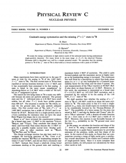
in Fig. 8 for 800.MeV protons scattered on a “%n target. The cross section obtained
from the free response is also shown. Note the enhancement of the total cross section
compared to the free response for low excitation enrgies. It is mainly due to the
I
I
/
OO
IO
20
4iw(MeV)
30
I
40
50
FIG. 8.
Experimental
) 12) and calculated
inelastic cross sections for 800-MeV
protons on ““Sn, at
a fixed laboratory
scattering
angle of 5 degrees. The two calculated
curves were obtained from the free
response of a semi-infinite
slab (dashed curve) and from the collective
responses. summing
(6.5) over all
spin and isospin channeis (solid curve).
274
ESBENSEN AND BERTSCH
FIG. 9. Experimental
I13 ] and calculated
inelastic cross sections for spin-flip
of 3 19.MeV polarized
protons
on 90Zr. at a fixed laboratory
scattering
angle of 3.5 degrees. The calculated
results were
obtained
from Eq. (6.6) using the field-free
response (dashed curve) and the collective
responses in the
S = I spin excitation
channels. respectively.
isoscalar response, which in fact dominates with more than 70% over the entire
energy range shown in the figure. The measured cross section [ 121 shows an even
larger enhancement for low excitation energies, with structures that are not contained
in the slab response.These structures are the well-known giant resonances,which are
specific properties of the finite geometry of the nucleus.
Recent measurementsof spin-flip cross sections [ 131 provide new information on
the residual interaction in the S = 1 excitation channels. The elastic cross section for
a spin-flip of the incoming proton is given in Appendix D, and the corresponding
inelastic cross section can be determined from the expression
(6.6)
spf=
summing over the S = 1 isospin channels. The predictions of the slab model are
compared with experimental results in Fig. 9 for 319.MeV protons on a 90Zr target.
Note the shift in the position of the maximum compared to the free response.This
shift originates from the residual interaction in the (T== 1, S = 1) excitation channel
which dominates the spin-flip cross section by about 70%. Within the mode1there
are no free parameters, so the absolute agreement is a successboth for the theory of
the response and the impulse approximation theory of the projectile-target
interaction. We also predict that the spin-flip cross section peak is just the region of
the current data.
7. CONCLUSIONS
The present investigation of the surface response of a semi-infinite Fermi liquid,
based on the Random Phase Approximation, illustrates some basic features of the
surface response of self-bound, interacting many-body systems. It is especially
relevant for the quasi-elastic scattering on heavy nuclei of high-energy probes that are
strongly absorbed in the nuclear interior.
SURFACE
RESPONSE
OF FERMI
LIQUIDS
215
The residual interaction in the isoscalar channel is partly determined by selfconsistency and partly from the range of the interaction in directions parallel to the
surface. Phenomenological
interactions
have been used for other spin-isospin
channels. The isoscalar response of the semi-infinite system exhibits a large enhancement at low excitation energies compared to the free response, with a significant
fraction of the energy-weighted
sum rule that is typical for the response of finite
nuclei.
Separable residual interactions
lead to quite reasonable response functions,
compared to more realistic interactions. The separable interaction has the advantage
that the associated collective response can be determined directly from the coupling
constant and the free response, which in the present study is quite well represented by
Lorentzian distributions.
A local Fermi gas model, based on the Green’s function of an infinite Fermi gas,
but suitably modified to describe the response of an inhomogeneous system, is rather
successful for large momentum transfers along the surface. For zero momentum
transfer, however, the model is unreliable to describe the surface response of the semiinfinite Fermi gas. In this case the much simpler model of an infinite Fermi gas is
more useful. In this model the isovector and the free response simulate the surface
response quite well, provided the density of the infinite system is chosen so that the
energy-weighted sum of the surface response is reproduced.
The finite range of the isoscalar residual interaction parallel to the surface has
some very significant consequences. In our formulation it enters into the separable
interaction through an effective coupling constant that depends on the momentum
transfer along the surface. It leads to a reduction of the interaction for a nonzero
momentum transfer, compared to the case of a zero-range interaction. Fluctuations in
the surface density of the interacting ground state are consequently also reduced.
Moreover,
the effective surface tension, extracted from the static isoscalar
polarization, is about 1 MeV/fm* and it is dominated by the contribution from the
finite range of the interaction along the surface, whereas the contribution from the
kinetic energy is surprisingly small.
The predominance of the isoscalar response at low excitations can explain the main
features of quasi-elastic scattering data for high-energy protons. The response in the
spin channels is also well reproduced, when a reasonable strength of the interaction is
included in the RPA calculation. The detailed structures
of giant resonances,
however, are not directly seen in the response of the semi-infinite system. If the aim
of the theory is to describe the overall behavior of the response, and not specific
resonant features, the semi-infinite slab model is very successful.
APPENDIX
The initial states of a semi-infinite
A:
FREE
RESPONSE
slab, with energies e, = (fiki)‘/2m,
Qi(r) = tii(z) exp(ik,r,).
have the form
(A.11
276
ESBENSEN
The z-dependent
equation
AND
part of these wave
HOz
4i(z)
where eiZ = (fiki,)‘/2m.
=
-
&
$
BERTSCH
functions
+
$i(z)
V(Z)
[
=
to the Schrodinger
64.2)
&iz #i(Z),
I
They can be normalized
$i(z) + fl
are solutions
to have the asymptotic
Cos(kizz + Oi),
behavior
for z + -03,
so that the spatial average value of 1Qij2 is unity in the interior
unperturbed density of the slab is
The subscript (F) on the integral indicates that all states below
included in the integration, and the factor of 4 accounts
degeneracy. The Fermi momentum is related to the density in
by 2ki/(3n2) =p,(-co)
= 0.16 fmP3.
We define the direct field-free Green’s function for the slab
(A-3)
of the slab. The
the Fermi surface are
for spin and isospin
the interior of the slab
as follows:
G:(r, r’, w)
=& 1
Fdki@~(r)(r~(H,-ei-hw-L4~‘Ir’)@i(r’).
The quantity A is greater
vanishingly small, but in
for A in order to improve
function used in Eq. (2.4)
(A-5)
than zero to ensure causality. It is usually considered as
some cases discussed in Section 3 we choose a finite value
the numerical convergence. The retarded field-free Green’s
is
G,(r, r’, co) = Gf(r,
r’, w) + (Gf(r,
The induced density due to an external perturbation
with the frequency o is given by
dp,,(r, w) = -
J
r’, -co))*.
U(r) that is oscillating
dr’ G,(r, r’, o) U(r’).
(‘4.6)
in time
(A.7)
Our system is translationally
invariant in the two directions parallel to the surface of
the slab. We can therefore Fourier transform with respect to the x - 4’ coordinates
along the surface, and obtain the equation
&,(z,K,w)=-
I’dz’G,(z,z’,K,w)CT(K,z’).
(A.81
SURFACE
RESPONSE
Here G,(z. z’, K, to) is constructed,
Gf(z. z’. K, tu) =
&.I,
I-
Ai
217
OF FERMILIQUIDS
as in Eq. (A.6). from the direct Green’s function
4itz)
#iCz’)
x:I,(H,,+~(K’+~K~,)-F;~-~~-~A)~‘,--’\.
(A.9)
which is seen to be independent of the orientation of K. We calculate the latter singleparticle Green’s function using the exact representation [ 14 1
2nz
(il(H,;-E-iA)~‘l;‘)=-h’W
~
u(z,) t’(Z)).
(A. 10)
The functions u and z’ are solutions to the equation H,,:d = (E + iA)d, obeying the
boundary conditions
u(z) + exp(-ikz).
where k = $%@
for z+--co,
(A.1 1)
for ~‘00,
(A.12)
+ iA)/h, and
P(Z) + exp(ikz).
where k = J2m(E+a
--V,)/h.
solutions: IV = UC’ - YIL’.
The quantity
APPENDIX
B:
FERMI
W is the Wronskian of the two
GAS
MODEL
For an infinite Fermi gas of nuclear matter the field-free Green’s function is
G,(r. c’. tu) = (2~) 3 1.dk G&k, CL))exp(zk(r - r’)),
(B.1)
where
Go+ w) = 41
(2n)j r dki((r;~;~ho-i71)~‘+(&,,+hw+i71)~~’}.
WI
and erj = (h’/2)7z)(k’ + 2kk,) and ki = (3rr2/2)p,,. The factor 4 takes care of spin and
isospin degeneracy. This function can be expressedin terms of the Lindhard functions
[ 151 as follows:
ESBENSEN AND BERTSCH
278
where ( = k/2k, and u = wjkv,. For a planar field Vext(z) the induced density
Gp,,(z,W) has the Fourier transform
Go% w> = -Go@, 0) V,,,(k)
(B.4)
and the free responseis
So(w)
= j$ ”i_cc
mdkIm{Go(k3
~11I~&)12.
P.5 1
The energy-weighted sum rule (2.24) can be expressed in a more detailed form for
each Fourier component of the external field as follows:
dooIm{G(k,w))=~po+
A2k2
P.6)
The self-consistent equation (2.4) can easily be solved in Fourier space, if the
residual interaction is of the folding type
7 ‘(r - r’) = (27~) 3.[ dk ?’ ‘(k) exp(ik(r - r’)),
P-7)
i.e., translationally invariant. The equation is then
Mk, w> = -G,(k,
o){ V,,,(k) + 7 ‘(k) 8~ (k. w)L
P.8)
and the imaginary part of the RPA Green’s function is
3Po
Im{Gkw.4@, WI1 = F
(1
f2
+ U,)’
+
oLfi)Z
’
where x = 3p,Y’ ‘(k)/(2&,). This function also obeys the sum rule (B.6). The
consist of two contributions, viz., one from the single-scattering region (f2
one from a collective mode (f, = 0 and 1 + xf, = 0). The contribution
collective mode is indicated in Fig. 6 for the isovector responseof a Fermi
APPENDIX
P.9)
sum may
# 0) and
from the
gas.
C: STATIC PROPERTIES
In this appendix we shall expand the static polarization to second order in the
momentum transfer along the surface, for the purpose of relating it to the surface
tension in Section 5. The algebraic manipulations are similar to those in Ref. 141,
where the quanta1 pressurewas related to the surface tension. The static properties of
SURFACE
RESPONSE
OF FERMI
the non-interacting ground state of a semi-infinite
function (cf. Eqs. (A.6) and (A.9))
279
LIQUIDS
slab is determined by the Green’s
Go@, z’, K, 0)
= &
(, dki 2#i(z) (z / (HO, + AEi - ei,)p’
‘I-
lz’)$itz’)3
(C.1)
where
AEi = ;
(K* + 2KkiI}
cc.21
is the energy loss associated with the momentum transfer hK in the s-direction
parallel to the surface. This function is a real function.
We first determine the induced density for a static and uniform displacement of the
surface. For a small displacement 6z the external field on the slab is -V’(Z) 62, and
the induced density (in units of 62) becomes
&Q,(Z) = 1.dz’ G,(z, z’. 0.0) I’.
(C.3 1
We can evaluate this expression using the commutation relation
i.e.,
(H,,, ~ Eiz)- ’ V’(z) fji(Z) = -&(z).
(C.5 1
From Eqs. (C.l) and (C.3) we thus obtain
(C.6)
which is the result stated in Eq. (2.16).
We shall now expand the static polarization function
P,(K) = f dz 1’dz’ V’(z) G,(z, z’, K, 0) V’(z’)
.
.
(C.7)
to second order in K. We therefore expand the inverse operator in Eq. (C.l) to second
order in AEi. Since we shall perform an integration over the Fermi sphere, we can
effectively use the approximation
(Ho; + AE; - eJ’
=: (Ho, - EJ’
-~j(Ho,--c,.)?-2~kt(ll,=-Ci;)-Jj.
I
(C.8
280
ESBENSEN AND BERTSCH
The first term yields the simple result
P,(K = 0) = .f dz V’(z) &,(z) = 1 dz p,,(z) V”(z).
(C.9)
Equation (C.5) can also be used to evaluate the contribution from the second term.
To evaluate the third term we make use of the commutation relation
From this relation and Eq. (C.5) we find that
(HOL - Eiz) -’ v’(z)
$i(Z)
=
~
(C.11)
Z~i(Z).
The static polarization function to second order in K is therefore
P,(K) = P,(K = 0) - 2K2 AT,
where
For a finite system we perform a partial integration so that ~z#~(z) if(z) is replaced
by -(#i(z))2. The quantity AT is then the difference between the kinetic energy (per
unit area) in the z-direction perpendicular to the surface and the kinetic energy in a
direction parallel to the surface.
APPENDIX
D: ELASTIC
SCATTERING
The general parametrization of the elastic nucleon-nucleon scattering amplitude
f(q) has the following form in the center of mass system [ 111:
(x&J’f(q)
=A + iqC(a,n + a*n)
+ Bo,o, + W,dhq)
+
Ea,;c~,,
PI)
where q represents the momentum transfer. The z-axis is here along the average
(initial-final) momentum direction, and n is a unit vector perpendicular to the
scattering plane. From the proton-proton (pp) and the proton-neutron (pn)
amplitudes, tabulated in [ 1l], we can determine the elastic isoscalar and isovector
amplitudes by
fM&l)
= If&l)
+ f,“W/27
P-2)
ST=I(S) = Lf,,(s> --fp”(qw~
(D.3)
281
SURFACE RESPONSE OF FERMI LIQUIDS
respectively. These amplitudes are again parametrized as in Eq. (D. 1). with coefficients A,. through E,. We can now construct the elastic cross sections for the
different spin-isospin excitation modesof the target. For the S = 0 channels one finds
that
and for the S = 1 channels one finds
Of particular interest is the cross section for a spin-flip of the incoming proton.
The elastic cross section for this process is given by the expression
= (2kcM)‘{lB,.+q2D,I’
+IB,+E7.121.
P.6)
T.SPf
ACKNOWLEDGMENTS
Valuable
We
also
discussions
acknowledge
with
support
J. W.
by
Negele,
the
National
0.
Scholten,
Science
and
P. J. Siemens
Foundation
under
are
gratefully
Grant
acknowledged.
PHY-80-17605.
REFERENCES
1. D. M. NEWNS. Phys. Rer. B 8 (1970), 3304.
2.
3.
4.
5.
6.
7.
8.
Y.
10.
I I.
12.
13.
14.
15.
Rec. B 12 (1975).
1319.
Phys. Rev. R 20 (1979). 3 186.
P. FEIBELMAN.
Ann. Physics 48 (1968),
369.
G. F. BERTSCH.
D. CHA, AND H. TOKI, Phys. Rev. C 24 (1981).
533.
G. F. BERTSCH. Progr. Theoret. Phys. 74-75 (1983).
115.
G. F. BERTSCH
AND S. F. TSAI, Phys. Rep. C 18 (1975). 126.
H. ESBENSEN AND G. F. BERTSCH. Phvs. Rep. C 28 (1983).
355.
T. IZUMOTO,
M. ICHIMURA,
C. M. Ko, AND P. J. SIEMENS.
Ph.vs. Leti.
G. F. BERTSCH
AND 0. SCHOLTEN.
Phys. Rec. C 25 (1982). 804.
S. J. WALLACE,
AWL,. in Nuclenr Phys. 12 (1981),
135.
J. M. Moss
er al.. Phys. Rec. Left. 48 (1982).
189.
S. K. NANDA
el al.. Phys. Rer. Left. 51 (1983). 1526.
P. FEIBELMAN.
R. G. BARRERA
C. MAHAUX
North-Holland,
J. LINDHARD,
Ph.vs.
AND
A. BAGCHI.
AND H. A.
Amsterdam,
Mat.-Fys.
WEIDENM~~LLER.
1969.
Medd.
Danske
“Shell
Vid. Selsk.
Model
Approach
28 (8) (1954).
B I I2 (1982).
to Nuclear
3 15.
Reactions.”
p.
I I.