1. Art and Diseño

The Spike Response Model: A Framework to
Predict Neuronal Spike Trains
Renaud Jolivet1 , Timothy J. Lewis2 , and Wulfram Gerstner1
1
Laboratory of Computational Neuroscience,
Swiss Federal Institute of Technology Lausanne, 1015 Lausanne, Switzerland,
{renaud.jolivet, wulfram.gerstner}@epfl.ch,
http://diwww.epfl.ch/mantra
2
Center for Neural Science and Courant Institute of Mathematical Sciences,
New York University, New York, NY 10003, USA,
[email protected],
http://www.cns.nyu.edu/˜tlewis
Abstract. We propose a simple method to map a generic threshold
model, namely the Spike Response Model, to artificial data of neuronal
activity using a minimal amount of a priori information. Here, data are
generated by a detailed mathematical model of neuronal activity. The
model neuron is driven with in-vivo-like current injected, and we test
to which extent it is possible to predict the spike train of the detailed
neuron model from that of the Spike Response Model. In particular, we
look at the number of spikes correctly predicted within a biologically
relevant time window. We find that the Spike Response Model achieves
prediction of up to 80% of the spikes with correct timing (±2ms). Other
characteristics of activity, such as mean rate and coefficient of variation
of spike trains, are predicted in the correct range as well.
1
Introduction
The successful mathematical description of action potentials by Hodgkin and
Huxley has led to a whole series of papers that try to describe in detail the
dynamics of various ionic currents. However, precise description of neuronal activity involves an extensive number of variables, which often prevents a clear
understanding of the underlying dynamics. Hence, a simplified description is desirable and has been subject to numerous works. The most popular simplified
models include the Integrate-and-Fire (IF) model, the FitzHugh-Nagumo model
and the Morris-Lecar model (for a review, see [1]).
In this paper, we make use of the Spike Response Model (SRM), a generic
threshold model of the IF type. Similar to earlier work [2], we map the SRM
to a detailed mathematical model of neuronal activity. But, in contrast of what
has been done in [2], we go beyond the classic Hodgkin-Huxley neuron model of
the squid axon and use instead a model of a cortical interneuron. Moreover, we
use a different mapping technique that could also be applied to real neurons. We
show that such a simple technique allows reliable prediction of the spike train of
O. Kaynak et al. (Eds.): ICANN/ICONIP 2003, LNCS 2714, pp. 846–853, 2003.
c Springer-Verlag Berlin Heidelberg 2003
The Spike Response Model: A Framework to Predict Neuronal Spike Trains
847
a fast-spiking interneuron. Prediction of up to 80% of spikes with correct timing
is achieved. The model also quantitatively reproduces the subthreshold behavior
of the membrane voltage (see Fig. 1) as well as other characteristics of neuronal
activity including mean rate and coefficient of variation (Cv ).
100
membrane voltage (mV)
Original model
SRM
0
-100
2000
2100
2050
2150
2200
time (ms)
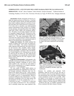
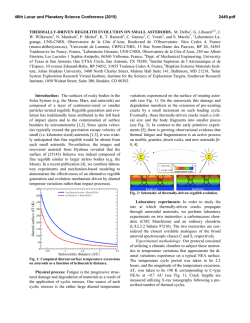
Fig. 1. The prediction of the SRM (dotted line) is compared to the target data (solid
line). The model achieves very good prediction of the subthreshold behavior of the
membrane voltage. The timing of all the spikes is predicted correctly, except that one
extra spike is added at around 2125ms.
2
Model
In this section, we describe the SRM in detail. The state of a neuron is characterized by a single variable u, the membrane voltage of the cell. Let us suppose
that the neuron has fired its last spike at time tˆ. At each time t > tˆ, the state of
the cell is written:
+∞
ˆ
u(t) = η(t − t) +
κ(t − tˆ, s)I(t − s)ds,
(1)
−∞
The last term accounts for the effect of an external current I(t). The integration
process is characterized by the kernel κ (additional external current). The kernel
η includes the form of the spike itself as well as the after-hyperpolarization
potential (AHP), if needed. As always, we have a threshold condition to account
for spike generation:
if u(t) ≥ θ and u(t)
˙
> 0, then tˆ = t.
(2)
848
R. Jolivet, T.J. Lewis, and W. Gerstner
Note that spiking occurs only if the membrane voltage crosses the threshold from
below. The threshold itself can be taken either as constant or as time-dependent.
We choose:
+∞
if t − tˆ ≤ γref
ˆ
,
(3)
θ(t − t) =
ˆ
θ0 + θ1 exp(−(t − t)/τθ ) else
where γref is a fixed absolute refractory period. θ0 , θ1 and τθ are parameters
that will be chosen to yield the best fit to a test dataset (target spike train).
The SRM is more general than the classic leaky IF model. In particular,
the choice of the kernel κ is not restricted. Moreover, κ is time-dependent since
it depends on the time elapsed since the last spike t − tˆ. Finally, the AHP is
described in a more realistic manner than in the leaky IF model where the time
constant of the AHP is equal to the membrane time constant.
3
Methods
In this section, we begin by generating a test dataset using a conductancebased neuron model stimulated by in-vivo-like time-dependent current. Then,
we explain the mapping of the SRM to the data, and finally, define how we
quantify the predictive power of the model.
3.1
Generation of the Test Dataset
The test dataset is generated with a Hodgkin-Huxley-like model. The model was
originally designed for fast-spiking interneurons [3] and was slightly modified for
the present study. Note that an analytical reduction from this detailed model to
the SRM is possible [1]. The model is integrated with a time step of 10−2 ms. The
driving current is a random Gaussian noise with constant mean µI and standard
deviation σI . During integration, the value of the current is changed every 20
time steps (= 0.2ms). The sampling frequency of our dataset is 5kHz. This highly
variable temporal input is thought to approximate well in-vivo conditions [4].
For each spike train, we record the membrane voltage and the driving current.
Both are needed later on.
3.2
Mapping of the Model
To realize the mapping of the SRM to the conductance-based neuron model, we
proceed in two steps. First, we extract the two kernels characterizing the model
(κ and η) and second, we choose a specific threshold (θ) and optimize it in terms
of quality of predictions.
Let’s start with the kernels. For the sake of simplicity, we assume that the
mean driving current is zero but the method can easily be generalized. We start
by extraction of the kernel η. It is well known that the shape of spikes is highly
stereotyped and presents only little variability. We therefore select one spike
The Spike Response Model: A Framework to Predict Neuronal Spike Trains
849
train from the dataset generated with the detailed model and align all spikes.
The mean shape of the spikes yields η. Detection and alignment of spikes is
realized using a threshold condition on the first derivative of the membrane
voltage.
Once we are done with η, we extract the kernel κ. Let us limit ourselves to
the interval between two consecutive spikes at times tj and tj+1 . Therefore, we
can rewrite equation (1) as follows:
u(t) − η(t − tˆj ) =
+∞
−∞
κ(t − tˆj , s)I(t − s)ds.
(4)
The right-hand side of equation (4) is the convolution product between the
driving current and a family of kernels κ parameterized by the variable t − tˆj . It
is then possible to find an approximation of the optimal kernel for each timing
by the Wiener-Hopf optimal filtering technique [5]. Let us consider each non-zero
term of κ as a free parameter and try to minimize the
squared distance between
data d(t) = u(t) − η(t − tˆj ) and prediction p(t) = s κ(t − tˆj , s)I(t − s) in a
time window centered on t − tˆj . Then, the optimal filter for that window is the
solution of the following linear system:

 


κ−N
C(d, I)−N
C(I, I)0
· · · C(I, I)M +N
 ···  = 
.

···
···
···
···
(5)
C(I, I)−(M +N ) · · · C(I, I)0
κ+M
C(d, I)+M
C(f, g)i is the numerical cross-correlation of vector f with vector g at lag i.
M (respectively N ) is the maximum positive lag (respectively negative lag) for
which κ is non-zero. It is obvious that this filter should be causal and therefore,
N = 0. Finally, we fit the resulting vector κ with a suitable function (usually an
exponential decay). The Wiener-Hopf method requires a window as large as the
support of κ. The result is that the dependency on t − tˆ cannot be reproduced
exactly. However, it is not a crucial point for correct prediction of the timing
of the spikes but only for correct prediction of the membrane voltage just after
emission of a spike, and only for time lags between 0 and about 30ms (for our
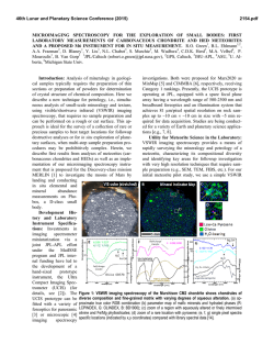
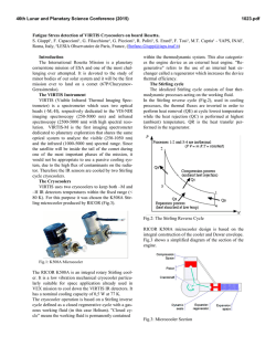
dataset). The kernels are plotted in Fig. 2.
The final step is to choose and optimize the threshold. The absolute refractory
period γref is set to 2ms. All the other parameters: θ0 , θ1 and τθ (see equation
(3)) are fitted in order to optimize the coincidence factor Γ using the downhill
simplex method (see subsection 3.3 for definition of this quantity).
For some technical reasons, we use three spike trains of 10s each to do the
mapping of the SRM to the detailed model. However, it is possible to do it with
only one spike train.
3.3
Evaluation of Predictions
Once we are done with the mapping, we simulate the conductance-based model
and the SRM with the same driving currents. These driving currents are new
850
R. Jolivet, T.J. Lewis, and W. Gerstner
B
A
-3
40
3×10
20
2 -1
κ (Ωm s )
η (mV)
0
-20
-40
-60
-3
2×10
-3
1×10
-80
-100
0
10
20
30
40
0
0
10
time (ms)
20
30
time (ms)
Fig. 2. Kernels extracted by the method described in text. A. Kernel η. B. Kernel κ
at different timings: t − tˆ = 0ms (dotted line), t − tˆ = 10ms (dash-dotted line) and
t − tˆ = 100ms (solid line).
and have not been used during optimization. Then, we count the number of
spikes in coincidence between both trains within a small time window ±∆. As
a measure of the quality of the prediction, we use the coincidence factor Γ [2]:
Γ =
Ncoinc − Ncoinc 1
2 (NSRM + Ndata )
1
,
N
(6)
where Ncoinc is the number of coincident spikes, Ncoinc is the mean number
of spikes that would be predicted correctly by a homogeneous Poisson neuron
firing at the same rate as the SRM (it can be calculated exactly), NSRM (respectively Ndata ) is the number of spikes elicited by the SRM (respectively by
the conductance-based model) and N is a normalization factor ensuring that
max(Γ ) = 1. Γ equals 1 if the spike train is predicted exactly and 0 if the
prediction is not better than a Poisson neuron (Γ can be lower than 0). The
denominator of the first term ensures that the mean frequency of both spike
trains is roughly the same.
4
Results
In this section, we show the predictions obtained from the SRM and quantitatively compare the results to the test dataset (target spike trains) generated using
the conductance-based model for fast-spiking intereneurons. Unless specified, we
used a dynamic threshold with θ0 = −49.1mV, θ1 = 14.9mV and τθ = 20.9ms.
We test the predictive power of the SRM by comparing the responses of the
conductance-based model neuron and the SRM to Gaussian noise current with
constant mean µI and standard deviation σI . Fig. 3 shows the effects of changing
The Spike Response Model: A Framework to Predict Neuronal Spike Trains
B
A
% of coincident spikes
1
0.8
Γ
0.6
0.4
0.2
0
0
10
20
30
40
50
60
100
70
80
60
40
20
0
0
10
20
2
C
40
50
60
70
50
60
70
σI (µA/cm )
D
1
80
0.8
60
0.6
Cv
mean rate (spk/s)
30
2
σI (µA/cm )
100
40
0.4
20
0.2
0
851
0
10
20
30
40
50
60
0
70
0
10
2
20
30
40
2
σI (µA/cm )
σI (µA/cm )
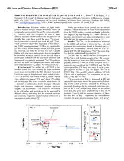
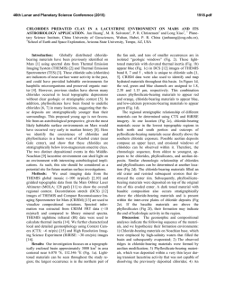
Fig. 3. The neuron is driven with zero mean Gaussian current. Panels A-D show results
of the SRM (solid line with squares). In addition, panels C and D show the target values
for mean rate and Cv (dotted line with circles). The arrows denote the point for which
parameters of the threshold have been optimized (same in the four panels). Mean of
five trials is plotted with two standard deviations for each point. A. Coincidence factor
Γ . B. Percentage of coincident spikes. C. Mean rate compared to target. D. Cv of the
interspike interval distribution compared to target.
variance with fixed mean, and Fig. 6 shows effects of changing mean with fixed
variance. In both cases, ∆ = 2ms and tested spike trains are 10s long.
prob. of occurence
1
0.8
Γ
0.6
0.4
0.2
0
5
10
15
20
25
30
2
σI (µA/cm )
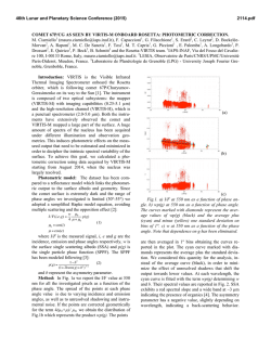
Fig. 4. SRM mapped to data at low rates
(here, between 7 − 35spk/s). Γ is plotted versus the current’s standard deviation σI (µI = 0). The arrow denotes the
point for which parameters of the threshold were optimized. The corresponding
rates are, from left to right, 7.6, 21.0 and
33.3spk/s. Here, parameters of the threshold are: θ0 = −52.5mV, θ1 = 37.5mV and
τθ = 5.2ms.
0.14
0.12
0.1
0.08
0.06
0.04
0.02
0
-20
-10
0
10
20
error of prediction (mV)
Fig. 5. Normalized histogram of the error of prediction of the membrane voltage. For each time step of one spike train,
we report the predicted voltage minus the
target voltage. The solid line is a fitted
Gaussian distribution centered on mean
µ = 0.6mV and with standard deviation
σ = 3.7mV. Effects at the tails are due to
missed and added spikes.
852
R. Jolivet, T.J. Lewis, and W. Gerstner
B
A
% of coincident spikes
1
0.8
Γ
0.6
0.4
0.2
0
-2
0
2
4
6
8
100
10
80
60
40
20
0
-2
0
2
4
6
8
10
8
10
µI (µA/cm )
D
1
100
0.8
80
60
Cv
mean rate (spk/s)
C
2
2
µI (µA/cm )
0.6
40
0.4
20
0.2
0
-2
0
2
4
6
2
µI (µA/cm )
8
10
0
-2
0
2
4
6
2
µI (µA/cm )
Fig. 6. The neuron is driven with varying mean Gaussian current. The current’s standard deviation is held constant at 25µA/cm2 . Panels A-D show results of the SRM
(solid line with squares). In addition, panels C and D show the target values for mean
rate and Cv (dotted line with circles). Mean of five trials is plotted with two standard
deviations for each point. The vertical dotted line is the limit of the subthreshold constant current. The threshold’s parameters are the same as in Fig. 3. A. Coincidence
factor Γ . B. Percentage of coincident spikes. C. Mean rate compared to target. D. Cv
of the interspike interval distribution compared to target.
The SRM produces very good predictions of the target spike trains over
a broad range of means and standard deviations of the injected current. The
model tuned using data at about 30Hz is still good for spike trains at 80Hz
(Fig. 3, panel A). If optimized for low rates, the SRM can also achieve good
performance of about Γ = 0.7 for σI = 10µA/cm2 (Fig. 4). Predictions hold in
the range 0-35Hz, which is roughly the range of interest for cortical pyramidal
cells. The subthreshold behavior of the membrane voltage is also very nicely
reproduced (see Fig. 1 and 5). Other standard quantities like the mean rate or
the Cv of the interspike interval (ISI) distribution are predicted in the correct
range, particularly the mean rate. This indicates that spikes that are missed or
added do not modify crucially the pattern of the spike train (Fig. 3, 5 and 6).
The SRM is very robust against some modifications. Predictive power is still
very good (Γ > 0.7) when using a shorter time window for coincidence detection
(∆ = 1ms) and using a constant threshold instead of a time-dependent threshold
reduces only slightly the range of validity of the model. On the other hand,
trying to simplify one of the kernel (η or κ) reduces significantly the quality of
predictions (data not shown).
The Spike Response Model: A Framework to Predict Neuronal Spike Trains
5
853
Conclusion
Prediction of the activity of neurons was attempted in the past. Keat, Reinagel,
Reid and Meister show that it is possible to predict the activity of neurons of the
early visual system [6]. However, these neurons produce very stereotyped spike
trains with short periods of intense activity followed by long periods of silence.
More recently, Rauch, La Camera, L¨
uscher, Senn and Fusi observed that an IF
model can reproduce the mean rate of neocortical pyramidal cells with the same
kind of in-vivo-like input current [7].
Here, we go one step further and propose a simple and general method to map
a threshold model to data of neuronal activity. Once the mapping is realized, the
model allows very reliable prediction of many aspects of neuronal activity, such as
timing of the spikes, membrane voltage, mean rate and Cv of the ISI distribution.
A posteriori, we may interpret the kernel κ as the response kernel of an IF model
with time-dependent time-“constant” [1]. The main advantage of this purely
numerical approach (compared to an analytical or semi-analytical approach) is
that it could, in principle, be extended to experimental data. Therefore, not
only do these results provide a basis for theoretical network studies on threshold
models, they also offer an approach toward studying the integration of inputs in
real neurons.
References
[1] Gerstner, W. and Kistler W., Spiking neurons models: single neurons, populations,
plasticity, Cambridge University Press, Cambridge (2002)
[2] Kistler, W., Gerstner, W. and Van Hemmen, L., Reduction of Hodgkin-Huxley
equations to a single-variable threshold model, Neural Comp. 9: 1015–1045 (1997)
[3] Erisir, A., Lau, D., Rudy, B. and Leonard, C., Function of specific K+ channels in
sustained high-frequency firing of fast-spiking neocortical interneurons, J. Neurophysiol. 82: 2476–2489 (1999)
[4] Destexhe, A. and Par´e, D., Impact of network activity on the integrative properties
of neocortical pyramidal neurons in vivo, J. Neurophysiol. 81: 1531–1547 (1999)
[5] Wiener, N., Nonlinear problems in random theory, MIT Press, Cambridge (1958)
[6] Keat, J., Reinagel, P., Reid, C. and Meister M., Predicting every spike: a model
for the responses of visual neurons, Neuron 30: 803–817 (2001)
[7] Rauch, A., La Camera, G., L¨
uscher, H.-R., Senn, W. and Fusi, S., unpublished
observations (2002)