
AN INVESTIGATION OF THE SPIN STRUCTURE OF THE
Nuclear Physics B328 (1989) 1-35
N o r t h - H o l l a n d , Amsterdam
AN INVESTIGATION OF THE SPIN STRUCTURE OF THE PROTON
IN DEEP INELASTIC SCATTERING OF POLARISED M U O N S ON
POLARISED PROTONS
The European Muon Collaboration
J. A S H M A N 12, B. B A D E L E K 15a, G. B A U M xTt', J. B E A U F A Y S 2, C.P. BEE 7,
C. B E N C H O U K ~, I.G. B I R D 5~', S.C. B R O W N 7d, M.C. C A P U T O 17, H.W.K. C H E U N G 1°~,
J.S. C H 1 M A l 1t, j. CIBOROWSKI15~ R. C L I F F T 11, G. C O I G N E T 6, F. C O M B L E Y ~2,
G. C O U R T 7, G. d ' A G O S T I N I s, J. D R E E S 16, M, D U R E N 1, N. D Y C E s, A.W. E D W A R D S 16g,
M. E D W A R D S l~ , T. E R N S T 3, M.I. F E R R E R O 13, D. F R A N C I S 7, E. G A B A T H U L E R 7,
R. G A M E T 7, V. G I B S O N mh, J. GILLIES 1°, P. G R A F S T R O M 14h, K. H A M A C H E R 16,
D.V. H A R R A C H 4, P.J. H A Y M A N 7, J.R. H O L T 7, V.W. H U G H E S 17, A. J A C H O L K O W S K A 2i,
T. J O N E S vk , E.M. KABUSS 3", B. K O R Z E N 16, U. K R O N E R ~6, S. K U L L A N D E R 14,
U. L A N D G R A F 3, D. L A N S K E l , F. L E T T E N S T R O M L4` T. L I N D Q V I S T 14, J. L O K E N m,
M. M A T T H E W S v, Y. M I Z U N O 4, K. M O N I G 16, F. M O N T A N E T 8h, E. N A G Y 6~, J. N A S S A L S K I t5
T. NIINIKOSK12, P.R. N O R T O N H, F.G. O A K H A M m ' , R.F. O P P E N H E I M tvn,
A.M. O S B O R N E 2, V. P A P A V A S S I L I O U 17, N. PAVEL 16, C. PERON113. H. P E S C H E L 16,
R. P I E G A I A Iv, B. P I E T R Z Y K 8, U. P I E T R Z Y K t6°, B. P O V H a, P. R E N T O N I°,
J.M. R I E U B L A N D 2, A. R I J L L A R T 2, K. R I T H 3c, E. R O N D I O 15~,
L. ROPELEWSK115a, D. S A L M O N 12k, A. S A N D A C Z TM,T. S C H R O D E R 3,
K.P. S C H U L E R Iv, K. S C H U L T Z E l , T-A. S H I B A T A 4, T. SLOAN 5, A. S T A I A N O ap, H.E. STIER ~,
J. S T O C K ~, G.N. T A Y L O R l°q , J.C. T H O M P S O N 11, T. W A L C H E R 4~, J.TOTH 6-i,
L, U R B A N 6~, W. W A L L U C K S 3, S. W H E E L E R ~2h, D.A. W I L L I A M S TM,
W.S.C. W I L L I A M S I°, S.J. W I M P E N N Y v~, R. W I N D M O L D E R S 9,
W.J. WOMERSLEY l°t, K. Z I E M O N S l
1111. Ph.rsikalisches hlstitut A, Phy'sikzentrum, R WTff, D-5100 Aachen, FRG
2CERN, CH-1211 Geneva 23, Switzerland
3Fakultiit fllr Phvsik, Universitgit Freiburg, D-7800 Freiburg, FRG
4Max Planck lnstitut fiir Kernphvsik, Heidelberg, FRG
5Department of Phvsicw, University of Lancaster, Lancaster LA1 4YB, UK
6Laboratoire d'Annecy-le- Vieux de Ptlvsique des Particules, F-BPl l O-74941,
Annecy-le- Vieux, France
VDepartnlent of Physics, University of Liverpool, Liverpool L69 3BX, UK
8('entre de Physique des" Particules, Facultd des Sciences" de Lumin.v, F13288 Marseille, France
'~Facultd des Sciences, Uni~'ersitd de l'Etat gz Mons, B 7000 Mons, Belgium
tllNuclear Phvsicw Laborato~', University of Oxford, Oxford OXI 3RH, UK
LIRuthepf~rd and Appleton Laboratory, Chilton, Didcot OXI OQX, UK
leDepartnlent of Pl[vsi~, UniversiO' of Sheffield, Sheffield $3 7Rll, UK
131stituto di Fisica, Universitdt di Torino, L10125, lta(v
t4Departnlent of Radiation Science, UniversiO' of Uppsala, S-75121 Uppsala, Sweden
l SPhvsics Institute, University of Warsaw and Institute for Nuclear Studies,
00681 Warsaw, Poland
t~'Fachbereich Pl~vsik, Universitiit Wuppertal, D-5600 WuppertaL FRG
J7Pto'sics Deparmwnt, Yale University, New Haven, Connecticut, USA
Received 30 May 1989
0550-3213/89/$03.50 ~ Elsevier Science Publishers B.V.
( N o r t h - H o l l a n d Physics Publishing Division)
J. Ashman et al. / Spin structure of proton
The spin asymmetry in deep inelastic scattering of longitudinally polarised muons by
longitudinally polarised protons has been measured in the range 0.01 < x < 0.7. The spin dependent structure function gi(x) for the proton has been determined and, combining the data with
earlier SLAC measurements, its integral over x found to be 0.126 _+0.010(stat.) + 0.015(syst.), in
disagreement with the Ellis-Jaffe sum rule. Assuming the validity of the Bjorken sum rule, this
result implies a significant negative value for the integral of g, for the neutron. These integrals
lead to the conclusion, in the naive quark parton model, that the total quark spin constitutes a
rather small fraction of the spin of the nucleon. Results are also presented on the asymmetries in
inclusive hadron production which are consistent with the above picture.
1. Introduction
O v e r the p a s t t w o d e c a d e s m a n y e x p e r i m e n t s h a v e s t u d i e d the s t r u c t u r e of the
n u c l e o n via d e e p i n e l a s t i c s c a t t e r i n g o f c h a r g e d l e p t o n s a n d n e u t r i n o s f r o m u n p o l a r i s e d t a r g e t s ( f o r r e c e n t reviews see ref. [1]). S u c h e x p e r i m e n t s h a v e e l u c i d a t e d the
quark-gluon
structure
of the n u c l e o n
and
have
shown
that
the q u a r k s
have
h a l f - i n t e g r a l spin. H o w e v e r , little i n f o r m a t i o n exists o n h o w the s p i n of the n u c l e o n
is d i s t r i b u t e d a m o n g its c o n s t i t u e n t s . S u c h i n f o r m a t i o n c a n b e d e r i v e d f r o m a s t u d y
o f d e e p i n e l a s t i c s c a t t e r i n g of p o l a r i s e d l e p t o n s o n p o l a r i s e d targets.
P r i o r to t h e p r e s e n t w o r k o n l y o n e such s t u d y h a d b e e n c a r r i e d out. T h i s was the
experiment
at S L A C u s i n g p o l a r i s e d e l e c t r o n s s c a t t e r e d f r o m a p o l a r i s e d p r o t o n
t a r g e t [ 2 - 4 ] . T h e e x p e r i m e n t d e s c r i b e d h e r e was d e s i g n e d w i t h a s i m i l a r o b j e c t i v e in
m i n d , b u t u s i n g a h i g h e n e r g y b e a m o f p o l a r i s e d p o s i t i v e m u o n s f r o m the C E R N
S P S w i t h a t a r g e t of p o l a r i s e d p r o t o n s . T h i s e x t e n d s c o n s i d e r a b l y the k i n e m a t i c
a University of Warsaw, Poland, partly supported by CPBP.01.06
b Permanent address: University of Bielefeld, FRG
c Present address: MPI fiir Kernphysik, Heidelberg, FRG
d Present address: TESA. S.A., Rennens, Switzerland
e Present address: University of Colorado, Boulder, Colorado, USA
f Present address: British Telecom, London, UK
Present address: Jet, Joint Undertaking, Abingdon, UK
h Present address: CERN, Geneva, Switzerland
i Present address: L.A.L., Orsay, France
J Permanent address: Central Research Institute for Physics of the Hungarian Academy of Science
Budapest, Hungary
k Present address: R.A.L., Chilton, Didcot, UK
I Institute for Nuclear Studies, Warsaw, Poland, partly supported by CPBP.01.09
m Present address: NRC, Ottawa, Canada
" Present address: AT&T, Bell Laboratories, Naperville, Illinois, USA
o Present address: MPI fiir Neurologische Forschung, KSln, FRG
P Present address: INFN, Torino, Italy
q Present address: University of Melbourne, Parkville, Victoria, Australia
r Present address: University of Mainz, Mainz, FRG
Present address: University of California, Riverside, USA
t Present address: University of Florida, Gainesville, USA
u Present address: UKAEA, Winfrith, Dorset, UK
J. Ashman et al. / Spin structure of proton
3
range of the observations and allows the spin structure of the proton to be studied
in detail.
In this paper the measurements of the spin dependent asymmetry in the cross
section for muon scattering are described, from which the spin dependent structure
function of the proton g l ( x ) is deduced. Here x is the fraction of the momentum of
the proton carried by the struck quark. The integral of gl(x) over x was used to test
the Ellis-Jaffe sum rule [5] and to investigate the contribution of the spin of the
quarks to the proton spin.
The final results presented here both extend and supersede those described in
previous publications [6-8].
2. The formalism of polarised deep inelastic scattering
The difference in the cross sections for deep inelastic scattering of muons
polarised antiparallel and parallel to the spin of the target proton can be written in
the single photon exchange approximation (for a review of the notation and
previous work see ref. [9])
d2o I"=
d2o
dQ2 dv ]
4~t~ 2
E202 [ M ( E + E'cosO)GI( Q 2, v) - Q2G2( Q2, v)],
(1)
where the variables are defined in table 1. The functions G I ( Q 2, ~') and G 2 ( Q 2, v)
are the spin dependent structure functions of the target nucleon. In the scaling limit
as Q2 and u become large these structure functions are expected to become
TABLE 1
Definition of the kinematic variables used
lepton rest mass
proton rest mass
D1
M
1
s = - - ( k , O , O , E)
lepton-spin four-vector
m
s=(o,s)
k=(E,k)
k'=(E',k')
P = (M,O)
q=kk'=(v,q)
Q2 = q2 = 4 E E ' sin2(0/2)
v=P-q/M=E
E'
0
x = Q 2 / 2 My
.v = v/E
proton-spin four-vector
four-momentum of incident lepton
four-momentum of scattered lepton
four-momentum of target proton
four momentum transfer
(invariant mass) 2 of virtual photon
energy of the virtual photon in the laboratory
scattering angle in the laboratory
Bjorken scaling variable
Bjorken scaling variable
4
J. Ashman et al. / Spin structure of proton
functions of x only [10] so that
M2vGl(Q2, v ) ~ g l ( x ) ,
Mv2G2(Q2, v ) ~ g 2 ( x ) .
(2)
These structure functions can be obtained from experiments in which longitudinally polarised muons are scattered from longitudinally polarised target nucleons by
measuring the asymmetry
do;l -do*t
A = d o T + + d o ~* "
(3)
This asymmetry is related through the optical theorem to the virtual photon
asymmetries A 1 and A2 by
A = D(A 1 + ~lA2) ,
(4)
where
01/2--03/2
A1 -
OTL
,
A 2 -
01/2+03/2
,
(5,6)
0T
y(2-y)
D=yz+2(1-y)(l+R)'
2(1-y)
B = y(2-y)
V~
~-
(7,8)
Here 01/2(%/2) is the virtual photoabsorption cross section when the projection of
the total angular momentum of the photon-nucleon system along the incident
1
lepton direction is ~£(~), o r = ~(Ol/2
+ %/2) is the total transverse photoabsorption
cross section and OTL is a term arising from the interference between transverse and
longitudinal amplitudes. The term R in eq. (7) is the ratio of the longitudinal to
transverse photoabsorption cross sections and D can be regarded as a depolarisation factor of the virtual photon.
The asymmetries A 1 and A 2 can be expressed in terms of the structure functions
gl and g2 [11] as
1
Al=(gl-'g2g2)-~l,
1
A2 = y ( g l -I- g2) ~1,
(9,10)
where F~ is the spin independent structure function of the proton (the explicit
(Q2, x) dependence of the structure functions has been omitted for brevity) and
y =(2Mx/Ey) ~/2. Hence eliminating g2 we obtain to first order in ~,, gl =
FI(A 1 + 7A2). Substituting for A 1 from eq. (4) gives
gl = FI( A/D + ( ~ - ~)A2)-
J. Ashman et al. / Spin structure of proton
5
There are rigorous positivity limits on the asymmetries [12], i.e. ]A~I _< 1 and
[A2] < ~ - . Since ~,, ~ and R are all small in the kinematic range of this experiment
the term in A 2 may be neglected and
(11)
m 1 ~- A / D ,
so that
(12)
gl = AtF1 = AIF2/2x(1 + R ) ,
where F 2 is the second spin independent proton structure function. Neglecting A 2
in this way is equivalent to neglecting the contribution of g2 which has been shown
to have a negligible effect [13].
The structure function gl(x) is obtained as follows. The asymmetry A (eq. (3)) is
obtained from the experimental data, from which the virtual photon asymmetry A 1
is deduced via eq. (11). The structure function gt(x) is then obtained from eq. (12)
using the known values of F 2 and R. The effect of neglecting A 2 is included in the
systematic error, using the above mentioned limits for A 2.
3. Theoretical models
By angular momentum conservation, a spin-1 parton cannot absorb a photon
when their two helicities are parallel. Hence in the quark-parton model (QPM),
01/2(03/2) can only receive contributions from partons whose helicities are parallel
(antiparallel) to that of the nucleon. Hence it follows that
Al
01/2
-
-
O3/2 -- E e 2 ( q [ ( x ) -- q[(x))
01/2 03/2
Ee2(qT(x) + q / ( x ) )
(13)
'
where q + ( ) ( x ) is the distribution function for quarks of flavour i and charge
number e, whose helicity is parallel (antiparallel) to that of the nucleon. The sum is
over all quark flavours i. In this model F 1 is given by
Fl(x ) = ~ _ , e ? ( q [ ( x )
+ q[(x)).
Hence from eqs. (12) and (13), it follows that
g l ( x ) : ½Y~e?(q + ( x ) - q [ ( x ) ) .
(14)
In the simple non-relativistic QPM [14] in which the proton consists of three
valence quarks in an SU(6) symmetric wave function, A p = ~ and A[' = 0 and are
independent of x. Such a model clearly did not describe the SLAC data. Many
models, mainly based on the QPM, were developed to predict the behaviour of the
J. Ashman et aL / Spin structure of proton
asymmetry A 1 (see ref. [9], for a review). Models giving a good representation of the
SLAC data were developed by Cheng and Fischbach [15], Callaway and Ellis [16],
Carlitz and Kaur [17] and Schwinger [18]. Most of these incorporate the perturbative QCD prediction [19] that A 1 tends to unity as x approaches unity and all
except [18] are based on the QPM. These models predict roughly the same
behaviour of A 1 and we choose arbitrarily to compare the data presented below with
the Carlitz and Kaur model.
4. Sum rules in polarised deep inelastic scattering
A sum rule was developed by Bjorken [20] from light cone current algebra and
with the assumption of quark structure for the hadronic electromagnetic and weak
currents. It relates the integral over all x of the difference of gl for the proton and
neutron to the ratio of the axial vector to vector coupling constants in nucleon beta
decay, gA" In the scaling limit it can be written
fol[glP(X)
-
-
g~l(x)] dx = 6~gA(1 -- %/¢r),
(15)
where the factor (1 - a s / ~ r ) arises from QCD radiative corrections [21]. This 1s a
fundamental sum rule which represents a crucial test of the QPM [22].
Separate sum rules for the proton and the neutron were derived by Ellis and Jaffe
[5] in a somewhat more model dependent approach. Assuming exact flavour SU(3)
symmetry in the baryon-octet decays and that the net polarisation of the strange
quark sea of the nucleon is zero, they derived
i g~(x) dx = -~- +1 +
.A[
5 3F/D - 1 ]
3 -k -YT-i ] '
1
ga[_l+
5 3F/D - 1 ]
3 T / f - Z - i 1'
fo
fo g;'(x)dx = 12 [
(16)
where F and D are the antisymmetric and symmetric SU(3) couplings [23].
Applying QCD radiative corrections to these yields [21]
lgp(n)(x)dx=-~-(_)
1--~-
+3
F~+-I
5-
1+433
2f
'
(17)
where f is the number of quark flavours.
J. Ashman et al. / Spin structure of proton
5. Experimental
7
procedure
The experiment was performed in the M2 polarised muon beam at the CERN
SPS using the EMC forward spectrometer [24] to detect the scattered muons and the
fast forward hadrons produced by deep inelastic scattering in a longitudinally
polarised target. For a fixed pion-to-muon energy ratio the muon beam was
naturally longitudinally polarised since the muon produced in the rest frame of the
parent pion has a fixed helicity. The polarised target [25] consisted of two cells filled
with ammonia, separated by a gap, with the free protons in each cell polarised in
opposite directions, parallel and antiparallel to the incident muon beam direction.
The free proton asymmetry was obtained from the difference in the count rates of
events reconstructed in each target cell. From this the asymmetry Al(x ) and the
structure function gt(x) were deduced.
Fig. 1 shows a schematic diagram of the apparatus. The trigger was provided by
the scintillator hodoscopes H1, H3 and H4 which selected muons scattered through
an angle greater than
x3 o. The scattered muon and forward hadrons were detected
and measured in the system of multiwire proportional (P) and drift chambers (W)
and their momenta analysed using a dipole field spectrometer magnetic (FSM).
Particles penetrating the 2.5 m thick steel absorber were labelled as muons. On
receipt of a trigger the chambers were read out and the data written onto magnetic
tape. These data were analysed using the EMC pattern recognition programme
( P H O E N I X ) and the momentum analysis and vertex reconstruction programme
( G E O M ) to write data summary tapes. The apparatus used in this experiment (fig.
1) is similar to that described previously [24] but was modified to run at the higher
beam intensities required. To achieve this the drift chambers in the high background
environment upstream of the magnet were replaced by proportional chambers (PV1,
PV2). In addition further small proportional chambers (POA-E), designed to work at
P~A
DLr
~]
F-F4
012
Fe
/
P4B
/
P5A
W4B WSB
I I I
3/.5m
Fig. 1, The EMC forward spectrometerfor the polarised-targetexperiment.
H4 H5
8
J. Ashman et a L / Spin structure of proton
high rates, were added in the beam region as well as the chambers P4/5. The latter
provided extra information in the central region of W 4 / 5 which had been found to
deteriorate after prolonged exposure to radiation due to the deposition of silicon on
the sense wires. With these modifications data were taken at beam intensities up to
4 x 10 v per SPS pulse of 2 seconds duration, repeated every 14 seconds, i.e.
approximately a factor 2 higher than previously.
Fig. 2 shows a schematic diagram of the polarised target. The two cells, each of
length 360 mm and volume l e °, were separated by a 220 mm gap. The target
material was in the form of approximately spherical beads of solid ammonia each of
volume - 4 mm 3, which allowed good cooling of the ammonia by the circulation of
liquid helium through the spaces around the beads. The two cylindrical cells were
positioned longitudinally along the beam line so that the same flux of incident
muons passed through each. Very precise monitoring of the beam flux was then
unnecessary since data were taken simultaneously for both directions of target
polarisation.
The free protons in the ammonia were polarised in opposite directions in each cell
by the method of dynamic nuclear polarisation. This method can be used for a small
range of hydrogenous materials, of which ammonia has the highest hydrogen
content. It requires that a dilute system of unpaired electron spins are introduced
into the material. Such paramagnetic centres had been previously produced in the
ammonia beads by irradiation with 25 MeV electrons at a temperature of 90 K,
using the injection linear accelerator at the Bonn electron synchrotron [25]. The
F=
5cm
-1
50cm
E
Cross Section
of Target
Dilution R~
Services
Radiation Shield
Vacuum
.,
Beam
•
8°
1
,,
m
/
Rapid Indium Seal
L
,:
Radiation Shields
/
Still
Liquid/Liquid
Heat Exchanger
Mylar Mixing
Chamber Wall
Microwave Cavity Wall
Dilution Refrigeration
Fig. 2. The polarised target.
/
Superconducting
Coils
J. Ashman et a L / Spin structure of proton
9
electron spins from the paramagnetic centres become highly polarised when the
material is placed in a strong magnetic field at a low temperature. This electron
polarisation can be transferred to the protons by microwave irradiation at a
frequency close to the electron spin resonance. The direction of the proton polarisation can be selected by making a small change ( - 0.6%) in the microwave frequency.
The magnetic field of 2.5 T was generated by a superconducting solenoid [26] of
length 1.6 m and internal diameter 190 ram, with its axis parallel to the muon beam
direction to obtain longitudinally polarised protons. The field over the target
volume was adjusted to be uniform to I part in 10 4 with the aid of 12 trim coils.
Such high uniformity was necessary to achieve resonance throughout the target
volume. Each target cell was mounted in a separate conducting cavity of 150 mm
diameter and supplied with microwave power at - 7 0 GHz from a separate
microwave source, allowing independent control of the polarisation direction.
The target material was maintained at a temperature of about 0.5 K, in the
presence of input from the microwave sources, by a 2 watt 3He 4He dilution
refrigerator [27]. The cooling system was common to both cells and so it was
necessary to include a series of thin copper baffles and some microwave-absorbent
material in the gap between the cells, to achieve isolation of the microwave power
whilst allowing a free flow of the coolant.
The proton polarisation was measured continuously during data taking with a
nuclear magnetic resonance system operating at a frequency of 106.3 MHz. This
system had eight independent channels and sampled the polarisation with four coils,
buried in the target material, in each cell. Calibration was carried out in the
conventional way, using the calculable signal which is obtained when the proton
spins in a known magnetic field are in thermal equilibrium with the solid lattice at a
known temperature. The statistical uncertainty on the measurement of the N M R
signal from a single coil was - 1 % . The mean polarisation of a target cell was
obtained by averaging the values from the four coils in that cell, which in general
agreed to within - 4 % . The overall error on this mean value arose from the
polarisation non-uniformity together with uncertainties in the absolute determination of the calibration temperature and drifts in electronics. Thus the mean cell
polarisation, which was typically between 0.75 and 0.80, had an overall estimated
uncertainty of +0.05.
In this experiment, which detected all final states inclusively, it was impossible to
discriminate between scattering from free protons and from the unpolarised bound
nucleons in the complex nuclei in the target. Thus the effective target polarisation
was reduced by a factor f. The value of f, the dilution factor (see subsect. 6.3), was
maximised by using ammonia as the target material since it has the highest
hydrogen content of the available materials. However, it suffers from the disadvantage of having a long polarisation reversal time ( - 8 h). For this reason, it was not
possible to reverse the polarisation directions more often than once per week
without unacceptable loss of data taking time. A further problem was that the 14N
10
J. Ashman et a L / Spin structure of proton
nuclei in the ammonia, which have spin 1, became slightly polarised [28], although
this produced a negligible correction to the final results (see subsect. 6.5).
The data were taken in 11 separate experimental runs at incident muon energies
of 100, 120 and 200 GeV. The apparatus acceptances from the two halves of the
target differed by about 10%. In order to correct for this and for the - 1 %
difference in the target masses in each cell the polarisations were reversed once in
each experimental run and the results before and after the reversal were averaged.
6. Data analysis
6.1. I N T R O D U C T I O N
The free proton asymmetry A (eq. (3)) is extracted from the difference in counting
rates of the events whose vertices were reconstructed in the two target cells. Fig. 3
shows a reconstructed vertex distribution along the beam direction together with the
cuts applied to define the events in each target cell. Using a Monte Carlo simulation
of this distribution, it was shown that the events could be assigned to each target
cell without ambiguity. The events reconstructed in between the target cells stem
from interactions in the residual material (copper baffles and helium) in the gap and
from the finite vertex resolution.
The measured event yields from the two target cells are
N u -- nubauoo(1 - - f P b P u A ) ,
(18)
N d = ndbad%(1 - f P b P a A ) ,
POSITIONS OF
TARGET HALVES
I
I
POSITIONS OF
VERTEX x CUTS
'?
1///// /////////~
L
I
t>
LL.I
0
0
0.5
I
1.I0
1.5
2.0
x (rn)
Fig. 3. Vertex distribution along the beam direction. The target edges and the applied cuts are shown.
J. A s h m a n et al. /
Spin structure of proton
11
where the subscript u (d) refers to the upstream (downstream) target half, n is the
number of target nucleons, b the beam flux, a the apparatus acceptance, % the
unpolarised cross section, f the fraction of the event yield from the polarised
protons in the target, Pb, Pu (Pd) the beam and target polarisations, respectively.
The phase space cuts on the beam ensured that the beam flux was the same for both
target halves. The sign of the polarisation of both target and incident muon is
defined to be positive when parallel to the incident positive muon beam direction.
With this definition Pb was always negative and Pu and Pd were of opposite sign.
For an experimental run where Pu was initially positive and Pd negative the
measured asymmetries are
N u - Nd
Nu + N d
Am
t
Am
_
N 2 - N2
_ _
N~ + N~
(19)
where the primed (unprimed) quantities refer to the quantities measured after
(before) the polarisation reversal during the experimental run. The free proton
asymmetry is related to the measured asymmetries by
A-m = ½(Am + A ' , ) = fPBPTA = fPBPTDA1,
(20)
where PB = IPb] and PT = (IPul + IPdl + Iedl + Iedl)/4 is the average target polarisation. Values of X m as a function of x for the total data sample are given in
table 5. The values are always less than - 0.02, so it was vital to control all possible
sources of systematic false asymmetries to much better than this figure. This was the
reason for having the split target design, since the uncertainty on the measurement
of the muon flux through the target was of the same order as the measured
asymmetry. All false asymmetries cancel from eq. (20) except those due to time
dependent acceptance changes. Such an effect would occur only if the ratio of the
upstream to downstream acceptance ratios before and after the polarisation reversal,
a u/a d
K = aJa~l
(21)
were different from unity. This would produce a false asymmetry which would
induce a systematic error in the results. This will be discussed later.
6.2. T H E B E A M P O L A R I S A T I O N
In the laboratory frame the muon polarisation is given by
~k--
m /2m , ~2( 1 - X)
P6 = -T X + ~ 2
,
m ; / m , , ( 1 - x)
(22)
12
J. Ashman et al. / Spin structure of proton
TABLE2
Beam-polarisationvalues calculated by Monte Carlo
Energy: E~/E. (GeV)
Polarisation
110/100
130/120
210/200
0.77 ± 0.06
0.79 ± 0.06
0.82 ± 0.06
where
X_
EtL--Emin
E~ - Emin '
with m , , m r the muon and pion masses, E~, E~ their energies in the laboratory
frame and Emin = ( m , /2m ~ ) E2~
is the minimum allowed muon energy in the laboratory frame. The negative (positive) sign is for positive (negative) muons. The beam
polarisation was computed by averaging eq. (22) over the beam phase space in a
M o n t e Carlo simulation of the beam [29]. Previous measurements of the beam
polarisation [30] agreed with the predictions of this Monte Carlo simulation within
measurement errors of 10 15%. Table 2 shows the computed beam polarisation for
each of the three settings used in this experiment. The quoted errors arise from the
uncertainties in the beam phase space and in the contamination of the parent 7r
b e a m by K mesons (18 _+ 9%).
6.3. THE DILUTION FACTOR
The dilution factor f is the fraction of the events arising from scattering by the
polarised protons in the target. To a first approximation f is 3/17 for the ammonia
( N H 3 ) target representing 3 free protons out of 17 nucleons per molecule. However,
several other effects must be taken into account. Firstly the neutron and proton
cross sections are not the same. Parameterising the available data [31, 32]* gives
(23t
% / % = 0.92 - 0.883x
with an uncertainty of - _+0.05 independently of x. Secondly, the cross section for
bound nucleons is not the same as that for free nucleons [33], the " E M C effect".
Parameterising the data for carbon [34], which is assumed to be similar to nitrogen,
h(x)
-
o (bound)
o(free) - 1 . 0 6 - 0 . 3 0 x - 0.45e
* Preliminary BCDMS results can be found in ref. [32].
44x
(24)
J. Ashman et al. / Spin structure of proton
13
The uncertainty in this ratio was taken to be either 0.03 or 0.5(1 - h(x)) whichever
is the larger. Thirdly, other material (helium and copper) within the target cells
contributed - 11% of the rate from the ammonia, with an estimated error of 20% of
its value, Fourthly, events originating from unpolarised material outside the target
cell contaminate the sample due to resolution smearing. This was estimated by a
Monte Carlo simulation to be (6.6 + 0.7)% with an estimated systematic error of 3%.
Taking all these effects into account the dilution factor becomes
f= 3 + h(x)(8.84 + 8.44%/%) "
(25)
6.4, T H E V I R T U A L PHOTON DEPOLARISATION FACTOR D
The factor D is defined in eq. (7). To compute it the values of R = OL/O T were
calculated using perturbative QCD [35]. These represent the measurements quite
well [1] within the rather large errors. Accordingly, an error equal to 50% of the
value calculated from QCD was assigned to R. A parameterisation of R calculated
in this way at the mean Q2 value in each x bin for this experiment is
R = 0 . 0 1 2 2 / ( x + 0.041) 1°96.
(26)
6.5. T H E C O R R E C T I O N S FOR RADIATIVE EFFECTS A N D THE N I T R O G E N POLARISATION
The quantities of interest, A 1 and gp (eqs. (11) and (12)) are defined in the onephoton exchange approximation, while the measured quantities contain contributions from higher-order processes and must therefore be corrected. The formulae of
Mo and Tsai [36] are used for these radiative corrections. Although the formulae are
strictly valid only for spin averaged cross sections the results are very similar to
those of a more exact treatment of Kukhto and Shumeiko [37]. The corrections also
included allowance for the slight polarisation of the nitrogen nuclei. In detail the
corrections were applied as follows.
The measured cross section om can be written as
Om(X ' y) = BkOly .q_ Oine
'R ..}_oR ,
(27)
where O'ly is the one-photon exchange cross section, B k is a correction factor to the
virtual photon flux for the vacuum polarisation, vertex graphs etc. and OinelR(O'elR) is
the contribution to the cross section in a given x, y bin from the inelastic (elastic)
radiative tails:
R
: y')dx'dy'
O.inel(el)R(X, y ) = f r(x', y ,,' x, y)Oinel(el)(X,
J. Ashman et al. / Spin structure of proton
14
Here r(x', y', x, y) is the probability that an event at x', y' appears, after radiating
one or more photons, in the bin x, y.
The measured asymmetry can then be written as
Bk + 7"1 + T2 + (P~/PT)(T3 + T4+ Ts+ T6) I
Am =fPBPTDA1
1 q- ( T 7 -}- T8) f
fPBPvDA1
l+Rc
)
(28)
'
where R c is the overall correction, PTN is the nitrogen polarisation (13% of the
proton polarisation PT [28]) and the different terms T~ are
T~: radiated asymmetry from the proton inelastic tail
T 1 - DAa°lv" f r(x ! , y ' , x , y ) D ( y ) At l ( x ) O ti n e l ( x t , y ' ) d x ' d y ' ,
(29)
with A 1 taken from a fit to the data.
T2: radiative asymmetry from the proton elastic tail. It is given by an expression
identical to eq. (29) but with the elastic asymmetry Ael (arising from the interference
of G M and G z, which have been determined to have the same sign [38]) substituted
for AI:
Ae, = De,(1 + ~ R~e,)
(30)
with
y(2 - y )
De,= y 2 + 2 ( 1 _ y ) ( 1 +Re1) ,
G~
Rel- rG2,
(31,32)
where G M and G E are the electric and magnetic form factors of the proton and
= Q2/4M2.
T3: correction for the asymmetry from the polarised nitrogen
oNA
T3 = B k
(33)
where o N, O"p, A N and A p are the cross sections and asymmetries for nitrogen and
proton, respectively. The asymmetry A N was computed using the shell model of the
nucleus in which the nitrogen nucleus consists of a spin-0 core of 6 protons and 6
neutrons plus an odd proton and neutron each in a p1/2 state so that the ground
state has spin 1. Writing down the nuclear wave functions shows that each odd
nucleon is twice as likely to have its spin opposite to the nuclear spin than parallel
J. Ashman et al. / Spin structure of proton
15
to it. Such a calculation predicts the static magnetic moments of 14N to within 10%
of the measured value. Thus neglecting the asymmetry from the odd neutron and
assuming that the bound and free proton asymmetries are the same A ~ - ~ ( o P / o N ) A p, so that T 3 - - B k / 9 . On multiplying this by the ratio P N / P T, the
polarisation of the nitrogen nucleus contributes a correction -1.5% to the free
proton asymmetry.
T4: Correction due to the inelastic radiative tail from the polarised proton in the
nitrogen (as in eq. (29), with A~ substituted for A1).
Ts: Correction for the quasi-elastic radiative tail from nitrogen.
T6: Correction for the coherent radiative tail from nitrogen.
T7: Total radiative correction for unpolarised protons.
Ts: Total radiative correction for unpolarised nitrogen. Here the single nucleon
cross section for carbon was used, which should be similar to that for nitrogen.
Fig. 4 shows the contribution of the various sources to the radiative correction.
The dash-dotted curve, labelled "polarised proton correction", is obtained from
0.4
- -
UNPOLARISED
--'--
POLARISEO
PROTON
CORRECTION
....
POLARISED
NITROGEN CORRECTION
CORRECTION
0.3
.~ 0.2
~o.1 \
I "
0
0.1
0.2
0.3
0.4
0.5
X
Fig. 4. Contributions from various sources to the radiative corrections: the curve labelled polarised
proton correction is B~ + T1 + ~ - 1 ,
that labelled polarised nitrogen correction is (pr~/px)×
(7~ + T4 + 7~s + T~) and that labelled unpolarised correction is f ( T v + Ts) (see text).
16
J. Ashman et al. / Spin structure of proton
0.8
-
0.7
O
-
MEAN
DEPOLARISATION
.......
MEAN
DILUTION
. . . . .
OVERALL
--
MEAN
-- --
RADIATIVE
VALUE
OF
FACTOR,
D
FACTOR,f
CORRECTION
Y
0.6
4---,
O
LL
cO
0.5
4.--'
O
(19
0.4
K.-
©
O
\\
0.3
0.2
\
0.1
\
'\
\
0
0
0L
.1
012
013
014
0.5
X
Fig. 5. The correction factors for radiative effects; depolarisation factor D; dilution factor f; ( y ) of the
data as a function of x.
B k + T t + T2 - 1 (eq. (28)). It shows the effect in the numerator of the asymmetry
arising from radiative smearing in elastic and inelastic scattering together with the
effects of the vacuum polarisation and vertex corrections. The term T2 from elastic
scattering is everywhere small. The dashed curve, labelled "polarised nitrogen
correction", is obtained from ( P ~ / P T ) ( T 3 + T 4 4- T5 + T6) which is dominated by
T3. The correction is rather small ( < 2% everywhere). The solid curve, labelled
"unpolarised correction" shows the term f ( T v + Ts) which represents the correction
to the unpolarised cross sections in the denominator of the asymmetry. The values
are dominated by the nitrogen contribution (Ts) which included quasi-elastic and
coherent elastic radiative scattering as well as the contribution from radiative
inelastic scattering and vacuum polarisation and vertex effects. The unpolarised
correction gives the largest contribution to the radiative corrections.
The total radiative correction to the measured value of A 1 (the term R c in eq.
(28)) is shown as a function of x in fig. 5. Also shown are the variation of the
depolarisation factor D, the dilution factor f , and the mean value of y.
J. Ashman et al. / Spin structure of proton
17
Electroweak effects were also studied but were found to be negligible in the Q2
range of this experiment.
7. Results
7.1. T H E V I R T U A L P H O T O N A S Y M M E T R Y A 1
The cuts applied to the data are given in table 3 and the numbers of events
surviving these cuts in table 4 together with other details of each experimental run.
The virtual photon asymmetry A 1 w a s calculated for each experimental run on a grid
of l l x and 15Q 2 bins. The data were then averaged in different ways. Table 5 and
fig. 6 show the values of A 1 as a function of x averaged o v e r Q 2 . The systematic
errors shown in table 5 are discussed below. The values of X 2 to the mean of each x
point for 10 degrees of freedom (11 runs) are also given. These show approximately
a statistical distribution which is evidence that systematic errors due to false
asymmetries are smaller than the statistical errors, provided that they do not always
TABLE 3
Kinematic cuts applied to the data for the three beam energies
L~
Q~,in
(GeV)
(GeV 2 / c 2 )
b'min
(GeV)
g~, min
(GeV)
.vm~×
0mi,,
100
120
200
1.5
2.0
3.0
10
10
20
18
20
30
0.85
0.85
0.85
1°
1°
1°
TABLE 4
Data used to measure the asymmetry
Run
(period, year)
2B84
2C84
2C84
3A84
3B84
3C84
3C84
2A85
2B85
2B85
2C85
I
II
I
II
I
II
Energy
(GeV)
Initial target
orientations
Mean target
polarisation, PT (%)
No. of events
after cuts × 10 3
200
200
200
120
200
200
100
200
120
200
200
/ +
- / +
+ / /+
+/
- / +
+/
/ +
- / +
+/ / +
77.3
78.5
75.5
74.4
78.7
79.0
80.7
80.5
72.7
71.7
78.4
114.6
62.5
68.7
236.3
115.8
44.1
202.1
41.5
180.5
58.5
97.5
J. Ashman et al. / Spin structure of proton
18
TABLE 5
A 1 in x bins
x range
0.01-0.02
0.02-0.03
0.03-0.04
0.04-0.06
0.06-0.10
0.10-0.15
0.15-0.20
0.20-0.30
0.30-0.40
0.40-0.70
Mean
x
0.015
0.025
0.035
0.050
0.078
0.124
0.175
0.248
0.344
0.466
AA 1
due to
Mean Q2
radiative Raw asymmetry"
( G e V / c ) 2 Mean D Mean f corrections
A-m
3.5
4.5
6.0
8.0
10.3
12.9
15.2
18.0
22.5
29.5
0.784
0.699
0.633
0.562
0.459
0.358
0.295
0.246
0.216
0.216
0.181
0.168
0.161
0.157
0.155
0.I58
0.163
0.171
0.183
0.199
0.005
0.005
0.005
0.005
0.004
0.004
0.005
0.007
0.011
0.017
0.0019
0.0063
0.0016
0.0050
0.0065
0.0065
0.0103
0.0140
0.0122
0.0167
+ 0.0030
4- 0.0031
4- 0.0034
+ 0.0027
-- 0.0022
+ 0.0025
+ 0.0026
4- 0.0028
4- 0.0036
+ 0.0048
At ± °,tat -- Osyst a)
0.027
0.091
0.026
0.082
0.141
0.181
0.363
0.458
0.525
0.638
+ 0.035
+ 0.042
4- 0.052
± 0.047
+ 0.047
4- 0.061
+ 0.084
i 0.086
4- 0.139
4- 0.172
x2/DOF
+ 0.010
+ 0.013
i 0.014
± 0.016
+ 0.021
+ 0.027
4- 0.037
+ 0,041
4- 0.045
± 0.049
7.7/10
7.3/10
5.2/10
5.0/10
4.5/10
21.4/10
15.2/10
12.0/10
8.0/10
9.1/10
aThere is an additional overall normalisation uncertainty of 9.6%, from the uncertainty in the beam and
target polarisations.
/
1.0
This experiment
0.8
)~ SLAC
[2]
SLAC
[3]
t
0.6
A~
0.4
0.2
0.0
-0.2
t
0.01
I
0.02
I
0.05
t
l
I
0.1
X
0.2
0.5
1.0
Fig. 6. T h e a s y m m e t r y A 1 for the p r o t o n as a function of x t o g e t h e r with the results f r o m p r e v i o u s
e x p e r i m e n t s [2, 3]. T h e c u r v e is f r o m the m o d e l of ref. [17].
J. Ashman et al. / Spin structure of proton
19
contribute in the same direction. A parameterisation of the data in fig. 6 is
A 1 = 1.025x°12(1 - e-2Vx).
(34)
The earlier data from SLAC [2, 3] are also shown in fig. 6. The agreement between
these data and the data presented here is good in the region of overlap. The new
measurements extend the range down to lower values of x. The solid smooth curve
in fig. 6 shows the predictions of the model of Carlitz and Kaur [17] based on the
conventional quark parton model. This model gives a good representation of the
data for x >_ 0.2 but fails to represent the new data at lower values of x. A recent
modification of this model, allowing the u and d quarks to have different masses,
obtained good agreement with the data over the whole x range [39]. Predictions of
the behaviour of A 1 with x were also made using the Fire String Model [40]. These
predictions are in good agreement with the data in fig. 6.
Fig. 7 shows the Q2 dependence of A 1 in three x ranges together with the older
SLAC data in the deep inelastic region [2, 3] and also in the resonance region [4] in
which a W cut (W > 1.31 GeV) has been applied to exclude the A33 (1236) resonance
1.0
B This ex0eriment
SLAC[2]
@ SLAC[3]
¢ SLAC[4)
0-8
0-6
0"4
0.01<x<
0"2
.
i,
0
-0"2
i
0.06
i~,i ,I, ++
J
t
,~,,,
1"0
0"06 <x< 0-20
0'8
0"6
A~ o-4
+
0.2
0
-0-2
I
i
i
;, ÷** ÷
+ +
,
,it,
I
I
i
J
l l l J t
i
,
J
t
, , l l
,
i
L
l , i i
1.0
0-20<x<
0.8
0.70
0.6
0-4
0-2
0
-0.2
t
0"1
i
i
i
i
i i/
I
i
i
i
i
1•0
i
i
t il
10
Q2 ( G e V / c ) 2
Fig. 7. A~ versus Q 2 in three x bins.
i
10(
J. Ashman et al. / Spin structure of proton
20
TABLE 6
Systematic errors for A n
Source of error
Total a
x
R
A2
K
f
Radiative corrections
systematic
0.015
0.025
0.035
0.050
0.078
0.124
0.175
0.248
0.344
0.466
0.001
0.003
0.001
0.004
0.005
0.004
0.009
0.008
0.006
0.005
0.003
0.005
0.007
0.008
0.012
0.015
0.019
0.021
0.023
0.022
0.009
0.010
0.012
0.013
0.016
0.020
0.025
0.028
0.030
0.027
0.002
0.005
0.00i
0.004
0.006
0.008
0.017
0.021
0.025
0.034
0.001
0.001
0.001
0.001
0.001
0.002
0.004
0.005
0.005
0.007
0.010
0.013
0.014
0.016
0.021
0.027
0.037
0.042
0.046
0.049
aThere is an additional 9.6% overall normalisation uncertainty arising from the errors in the beam and
target polarisations.
where the asymmetry is observed to be negative. This figure shows that there is no
strong Q2 dependence in the data. However, the predicted scaling violations due to
Q C D effects [41] are much smaller than the precision of the data. This negligible Q2
dependence of A 1 at fixed x allows us to combine the data taken with different
b e a m energies in the same x bin.
7.2. T H E SYSTEMATIC ERRORS ON A l
The systematic errors on A 1, shown in table 5, were evaluated from each of the
individual sources shown in table 6. The value of R used to compute the depolarisation factor was taken from a Q C D calculation [35] with a 50% uncertainty as
explained above (subsect. 6.4). The change in the value of A t as the computed value
of R is changed by 50% are shown in the second column of table 6 and this is taken
as the uncertainty due to R. Similarly the uncertainty due to the neglect of A 2 in eq.
(4) was obtained by recalculating A 1 assuming A 2 c a n be anywhere within the limits
- v r R < A 2 < f R , set by positivity requirements [12]. Taking R from the Q C D
calculation, as above, the changes in A 1 produced by neglecting A 2 in this way are
shown in the third column of table 6.
The dilution factor f (eq. (25)) suffers from uncertainties as described in subsect.
6.3. The total error on A 1 induced by these errors on f are shown in the fifth
column of table 6.
The uncertainties in the radiative corrections reflect both theoretical uncertainties
and those due to approximations made when applying the corrections to the data.
The uncertainty assigned was 15% of the correction or 1% of the measured value of
Y. Ashman et aL / Spin structure of proton
21
A1, whichever was larger. Due to the smallness of the correction itself, this is a
relatively unimportant source of error for A1. It is shown in column 6 of table 6.
The uncertainty labelled K in column 4 of table 6 is an estimate of the error
arising from possible false asymmetries due to time dependent changes in the ratio
of the upstream to downstream acceptances (au/ad). This is quantified by K, the
term defined in eq. (21). If K is not exactly unity, then the measured asymmetry (eq.
(20)) becomes, to first order in K - 1,
A,-
, [l ( A m + A ~ n ) +
fpspT~
-~-
,
where the + ( - ) sign is for periods of type 1(2), i.e. those in which the initial target
configuration is - / + , i.e. Pu < 0, Pa > 0 ( + / - ,
i.e. Pu > 0, Pd < 0). Fig. 8 shows
the values of A t as a function of x for the data averaged over the seven periods of
type 1 and over the four periods of type 2. The fact that the data for type 1 periods
tend to have larger values of A t than those for type 2 shows that K is not exactly
unity. The values of K in each x bin required to reconcile the differences in fig. 8
was determined using eq. (35). These values turned out to be constant within errors,
i.e. independent of x with a mean value of 0.990 _+ 0.005. In doing this the mean
value of K in each x bin was assumed to be the same for the 7 type 1 periods as the
4 type 2 periods. An approximately time independent value of K is expected since
1.0
~, Type 1 periods
J
Type 2 periods
0.8
0.6
0.4
0.2
0.0
-0.2
I
0.01
I
0.02
1
0.05
__1
0.1
I
I
0.2
0.5
1.0
X
Fig. 8. Comparison of the asymmetries Ap obtained from periods with the two possible initial polarisec
target configurations.
J. Ashman et al. / Spin structure of proton
22
the ratio a u/aa tended to increase uniformly with time due to the radiation damage
to the chambers in the beam region.
Since seven periods were of type 1 and four of type 2, there is a partial
cancellation of the false asymmetry term _ + ( K - 1 ) / 4 in eq. (35) when all eleven
periods are combined together. The above value of K of 0.990 4-0.005 for each
period becomes an effective Kto t of 0.998 + 0.001 when all periods are combined
together. To check this result the data were split into two subsamples for one of
which time dependent changes in the ratio a u / a d were expected to be much smaller
than for the other. Thus the asymmetry A x was determined for the subsample of
events in which the scattered muon passed outside the radius of P4/5. The values of
A 1 for this subsample were consistent within the errors for type 1 and type 2
periods. This was expected since no change in chamber efficiencies outside this
radius could be detected, and hence it can be assumed that the value of K for these
events is close to unity. Labelling A1 for this subsample as Aout, and for the total
event sample as Atot, we then have
Kto t - 1 = 4 f P B P T D ( A o u t - A t o t ) .
(36)
The points derived from the above equation are shown in fig. 9 as a function of x.
The values of K,o t are everywhere consistent with unity and have an average of
0.06
0.04
0.02
_
0.00
t__+__
-0.02
-0.04
-0.06
0.01
~
0.02
L
0.05
0 .' 1
,
0.2
0 .~0 5
1.0
X
Fig. 9. The measured value of K - 1 obtained by comparing the asymmetries measured for events with
muon tracks detected outside the chambers P4/5 and the total sample.
J. Ashman et al. / Spin structure of proton
23
1.003 + 0.002 in reasonable agreement with the previous value of 0.998 _+ 0.001.
Since both these values are consistent with unity, it was decided to take K t o t = 1.000
+ 0.003, constant and independent of x. Hence no systematic correction was
applied to the values of A l, but the above uncertainty was translated into a
systematic error on At, where values are shown in the fourth column of table 6.
As a consistency check on the above analysis events were selected which contained an identified hadron. For this sample the radiative corrections were small
since all the effects concerning the elastic radiative tail disappear on demanding a
hadron. In addition for such events a u / a a ~ 0.8 averaged over x compared to about
1.1 for the total inclusive sample. Thus any time dependent changes in a u / a d would
be expected to have a different effect between the two samples. Particles were
identified as hadrons and not electrons by demanding that less than 85% of their
total energy was deposited in the upstream electromagnetic part of the calorimeter
(H2 in fig. l). Fig. 10 shows the variation of A~ as a function of x for events with
accompanying hadrons compared to the values from the total sample. There is a
good consistency between the two sets of data, illustrating that the radiative effects
had been correctly calculated and residual false asymmetries were small compared
to the errors.
The data were split into two different subsamples in many other ways. None of
these gave a mean value of K which was significantly different from unity.
1.o I
J
08 iI
Ii
INCLUSIVE
ASYMMETRY
+ EVENTS CONTA,NI.G A HADRON
--
CARLJTZ £1nd KAUR MODEL
I
o
h
H
7
0.4
O
--
--
I
-o.21
o:ol
0.'02
o-o5
dl
0'.2 --
0'.5
.0
X
Fig. 10. Comparison of the asymmetries AIp as a function of x for events with one or more detected
hadrons with those from the total data sample. The smooth curve shows the prediction of the model of
ref. [17].
24
J. Ashman et at / Spin structure of proton
7.3. S E M I - I N C L U S I V E A S Y M M E T R I E S IN T H E F I N A L STATE H A D R O N S
Spin asymmetries for positive and negative hadron production were also measured. Here the asymmetries are given by
A±=
(do
±/dz)l/2- (do±/dz)3/2
(do
±/d2)1/2
+
(do
±/dz)3/2
(37)
'
where again the subscripts refer to the projection of the total angular momentum of
the virtual photon proton system along the incident lepton direction and the + ( - )
signs refer to positive (negative) hadrons. In the naive quark parton model A ÷ is
expected to be larger than A . This can be understood as follows. From helicity
conservation the cross section for quark scattering oq/2 is zero and u (d) quarks
fragment more readily to ~r+(~r ) mesons, particularly at higher z [42], where
z = E,Jv
with E, the pion energy. Thus if the u (d) quarks are polarised parallel
(ant±parallel) to the proton spin as expected in the naive quark parton model A +
should be larger than A - at higher z. Detailed calculations based on this model
were made by He±mann [43].
In order to maximise the difference between A + and A z should be as large as
possible. The analysis was performed with z > z 0 with z 0 = 0.1 as a compromise
between sufficient statistical accuracy and maxim±sing the expected differences
between A + and A - . The analysis procedure is identical to that for the inclusive
asymmetries described above except for the calculation of the dilution factors. This
stems from the different probabilities for a proton and neutron in the target to yield
TABLE 7
Semi-inclusive asymmetries in x bins (z > 0.1)
(Q2)
x range
(x)
(GeV2/c 2)
(D}
<f)
A + ± O~tat+ Os~s t
0.01-0.03
0.03 0.06
0.06-0.15
0.15-0.30
0.30-0.70
0.020
0.044
0.097
0.203
0.376
4,2
7,6
12,9
22,7
42.0
0,713
0.582
0.440
0.379
0.386
0,177
0.164
0.165
0.177
0.195
0.122
- 0.114
0.178
0.527
0.780
0.01-0.03
0.03-0.06
0.06-0.15
0.15-0.30
0.30-0.70
0.020
0.044
0,098
0.203
0.371
4,2
7.7
12.9
22,4
41.1
0.718
0.584
0.444
0.374
0.379
0.172
0.157
0.156
0.164
0.178
0.021
0.012
0.002
0.269
0.562
_+ 0.057
_+ 0.065
± 0.065
± 0.104
+ 0.214
±
+
+
+
+
0,028
0.033
0.043
0.051
0.046
x2/DoF
9.3/10
17.6/10
7.6/10
7.5/10
16.1/10
A ± °star ± °$st
+ 0.064
i 0,074
± 0,077
+ 0,131
+_ 0.283
_+ 0.024
+ 0.033
+ 0.043
+ 0.051
+ 0.047
9.9/10
19.1/10
11.2/10
5.9/10
ll.0/10
~There is in addition an overall normalization uncertainty of 9.6% (the same for A ~, A ) from the
uncertainties in beam and target polarisations.
25
J. Ashman et al. / Spin structure of proton
1.o
0.8
A+
0.6
A+o.4
0.2
+
+
0.0
-0.2
0.07
o. 2
o.85
o.'1
x
0.2
01s
1.0
Fig. 11. The semi-inclusiveasymmetries A ~(A-) for positive (negative)hadrons versus x.
final state ~r+ and ~r mesons. These dilution factors were computed from the
quark parton model using the quark distribution function taken from ref. [44] and
the parameterisations of the favoured and unfavoured fragmentation functions
taken from ref. [42]. The results are shown in table 7 and fig. 11.
It can be seen from fig. 11 that both A + and A rise at large values of x. This is
to be expected from the observed behaviour of the inclusive asymmetry (subsect.
7.1). However, the values of A + tend to be larger than those of A -, consistent with
the expectations of the naive quark parton model.
8. The structure function gP
The structure function gP was determined at a fixed Q2 = 10.7 GeV 2, the mean
Q2 of the data, using eq. 0 2 ) and the values of A a from table 5. As shown in this
table, the mean Q2 for these values varies considerably with x , but (from subsect.
7.1) there is no change of A 1 with Q2 at fixed x within the errors. The values of F 2
were taken from a parameterisation of the EMC hydrogen data [45] adjusted from
the value of R = 0 which was assumed in this parameterisation, to R calculated
from QCD. Table 8 and fig. 12 show the values obtained for gP together with the
systematic uncertainties described in sect. 7. The total normalisation uncertainty of
14% arises from 9.6% due to the uncertainty in the beam and target polarisations
and an assumed 10% due to the uncertainty in F~.
J. Ashman et al. / Spin structure of proton
26
TABLE 8
Final results for the spin-dependent structure function glv
Systematic error due to
x
gP
Statistical
error
0.015
0.025
0.035
0.050
0.078
0.I24
0.175
0.248
0.344
0.466
0.279
0.564
0.115
0,254
0,280
0,225
0.311
0.253
0.167
0.094
0.361
0.260
0.230
0.146
0.093
0.076
0.072
0.048
0.044
0.025
R
A2
K
0.014
0.026
0.004
0.004
0.005
0.005
0.003
0.003
0.002
0.001
0.046
0.029
0.02i
0.015
0.009
0.005
0.003
0.002
0.001
0.000
0.093
0.062
0.052
0.040
0.032
0.025
0.021
0.015
0.010
0.004
. f
0.018
0.031
0.004
0.009
0.012
0.010
0.014
0.011
0.008
0.005
Radiative
correction
Total
systematic
error
0.009
0.006
0.004
0.003
0.002
0.002
0.003
0.003
0.002
0.001
0.106
0.080
0.057
0.044
0.036
0.028
0.026
0,019
0.013
0.007
aThere is an additional overall 14% normalisation uncertainty due to uncertainties in beam and target
polarisations and in the value of F2,
+ This experiment
+ SLAC [2]
~L SLAC [3]
~r'
0.8
06[
g~(x)
0.4
_
_ -
_ _ _ I
0.2
I
I
I
1
1
I
0.01
0.02
0,05
0.1
0.2
0.5
1.0
Fig. 12. The structure function g P ( x ) as a function of x. The dashed curve is the value deduced from the
parameterisation (eq. (34)).
27
J. Ashman et al. / Spin structure of proton
The value of F2/(1 + R) for x < 0.03 was taken to be constant as expected from
Regge theory [46] and as confirmed experimentally up to Q 2 = 7 GeV 2 [471. The
d a t a in fig. 12 tend to be constant (within errors) for x < 0.2 as predicted from
simple Regge theory [46, 48].
9. The integral of gP over x
9.1. THE EMC DATA ALONE
In integrating gP over x the values of A 1 were assumed constant over each x bin,
but the function F 2 / 2 x ( 1 + R ) was integrated numerically for each bin because of
its rapid variation for x > 0.3. Fig. 13 shows the values of this integral from the low
edge of each bin to x = 1, plotted against the low edge of the bin, together with the
data f r o m S L A C [2, 3]. The inner and outer error bars are the statistical and total
errors. It should be noted that the errors are cumulative, i.e. each error contains the
c o n t r i b u t i o n from all the previous points at higher x. The normalisation error is
included in the total error. The smooth curve is the integral obtained by using the
parameterisation of A 1 (eq. (34)) which was used to estimate the contributions from
the regions in x not covered by the data, i.e. x < 0.01 and x > 0.7.
It can be seen that contributions from the lower x bins are small and the integral
converges well. The values of the integral shown in fig. 13 were obtained using a
fill
iI, This e x p e r i m e n t
SLAC [ 2 - 3 ]
ELLIS-JAFFE SUM RULE
0.15[X
"-¢3
" ~ 0.12
03
I~
~_..... x 0.09
0.06
0.03
0.01
I
I
1
I
0.02
0.05
0.1
0.2
t+?.O.o
0.5
1.0
Xm
Fig. 13. The convergence of the integral f),,gF dx as a function of x m, where x m is the value of x at the
low edge of each bin.
28
Y. Ashman et al. / Spin structure of proton
TABLE 9
The integral of g~ using different measurements of the unpolarised structure function
Source of ~
dx at Q2 = 10.7GeV 2
£ ~).v
.Olglp
EMC proton [45]
EMC iron [50]
DFLM [44]
BCDMS [51]
mean
standard deviation
0.113 -t 0.012
0.115 ± 0.012
0.123 ± 0.013
0.127 ± 0.014
0.120
0.0068
parameterisation of the E M C measurements of F 2 for the proton [45]. Recently,
some differences between the various measurements of F 2 have been highlighted
[49]. T o test the sensitivity to F 2 the integral was evaluated using the different
available d a t a on F 2. The results in the measurement region 0.01 < x < 0.7 are
shown in table 9 at Q2 = 10.7 GeV 2, the mean Q2 of the data. The first two values
of F 2 are the E M C proton [45] and iron data [50] where in the latter a correction has
been m a d e for nuclear effects on the nucleon structure function [33, 34] and for the
ratio of % / % from eq. (23). The entry labelled D F L M in table 9 uses the value of
F 2 c o m p u t e d from the most recent parameterisation of the neutrino structure
functions [44] which are based on data down to x = 0.015. The entry labelled
B C D M S is from a parameterisation of the data given in ref. [51]. To extrapolate the
latter data set below their measurement region (x < 0.06) the assumption was made
that FJ(1 + R) approaches a constant below x = 0.06 as discussed in sect. 8.
T a k i n g the mean of the values in table 9 gives
f0.olg
07 1p d x = 0.120 + 0.013 (stat.),
(38)
with an uncertainty due to F 2 = 5.6% which is taken from the standard deviation of
the values in table 9.
T h e contributions outside the measured region were obtained from the parameterisation of A 1 (eq. (34)) and these give
fo .7g,p d x = 0 . 0 0 1 ,
fO.Ol g,p = 0 . 0 0 2 .
J0
(39)
In the latter we assume that both gl and F2/(1 + R) are well behaved, i.e. remain
a p p r o x i m a t e l y constant as x approaches zero. For gl this is compatible with the
d a t a (fig. 12) and it has been shown to be true for F 2 up to Q2 _ 7 GeV 2 in a recent
experiment [47]. We assign errors equal to the values in eq. (39).
29
J. Ashman et al. / Spin structure of proton
TABLE l0
Systematic errors on the integral of gl
dilution factor f
uncertainty in RQ(, D
radiative corrections
neglect of A 2
beam polarisation
target polarisation
uncertainty in ~
acceptance effects
extrapolations into unmeasured region
± 0.0054
± 0.0007
_+0.0016
+ 0.0030
_+0.0092
+ 0.0074
+0.0071
_+0.0108
_+0.0030
total systematic error
± 0.019
The systematic errors affect the values in all the bins in the same way. The
contribution to the total uncertainty from each separate source is estimated by
recalculating the integral after increasing or decreasing all the points simultaneously
by the corresponding systematic error. Table 10 summarises the results together
with the global uncertainty which is obtained from the quadrature sum of the
individual contributions. Thus from the asymmetry measurements presented here
the integral becomes
f gt
1
P
__
--
d x = 0.123 + 0.013 + 0.019,
(40)
where the first is the statistical and the second the systematic error.
9.2. COMBINATION OF THE EMC AND SLAC DATA [2, 3]
Since we have already shown (fig. 7) that there is no indication of a Q2
dependence of A 1, over the range covered by the EMC and SLAC data, it is
reasonable to combine the results to achieve higher accuracy. Averaging over the
different sources of F2, as above, the SLAC data give
f0 .107glP d x = 0.094 + 0.008 + 0.014
_
_
(41)
and in the same region (0.1 < x < 0.7) the EMC data give
f0
°VgP d x = 0.090 _+ 0.010 _+ 0.011,
(42)
.1
where the contribution to the systematic error from the uncertainty in F 2 has been
excluded.
30
J. Ashman et al. / Spin structure of proton
The systematic errors in the two results have different origins, being dominated
by the uncertainty due to possible false asymmetries from acceptance effects in the
E M C case and by the value of R in the SLAC case. Therefore the systematic errors
can be combined as if they were statistical, giving
f °7gPdx = 0.092 ± 0.006 _+ 0.010,
(43)
0.1
where a further 5% contribution has now been added for the uncertainty in F 2 in
this x range. In addition the EMC data alone give
f0 .01g
.1 IP
d x = 0.030 + 0.008 +_ 0.007,
(44)
where the systematic error includes the uncertainty in F 2. In combining eqs. (43)
and (44), care must be taken regarding the correlation in the uncertainties for EMC
data in the low and high x ranges. If the systematic errors in eqs. (43) and (44) were
uncorrelated, they should be added in quadrature whereas if they were correlated
they should be added linearly. Since eq. (43) was obtained with approximately equal
contributions from SLAC and EMC, the mean of the values of the two approaches
is taken. Adding the contributions from extrapolating into the unmeasured regions
gives
foLgPdx
= 0.126 + 0.010 _+ 0.015.
(45)
The value expected for this integral from the Ellis-Jaffe sum rule (17) is
0.189 ± 0.005 using the current values of F/D = 0.631 _+ 0.018 [52], gA = 1.254 +_
0.006 and a~ = 0.27 _+ 0.02 at Q2 = 10.7GeV 2. The measured value is inconsistent
with this prediction.
IO. Discussion of the results and conclusions
The Q C D corrected parton model expression for the integral of glp can be
written [53]
Fp= ~glPdX=
1-
+
+2
1
a o , (46)
where the aj are directly related to the proton matrix elements of the nonet of axial
vector currents A~ = ' t ' y " % ( X i / 2 ) ' t", j = 0, 1 . . . . 8 by <P, SIA~IP, S> = 2MajS ~
where S ~ is the covariant spin vector of the proton.
J. Ashman et al. / Spin structure of proton
31
F r o m isospin invariance it follows that [20]
a3 = gA = F + D = 1.254 ± 0.006.
(47)
Furthermore, if SU(3)F is a good symmetry for describing the/3 decays of the octet
of b y p e r o n s [5]
a 8= (1/7~-)(3Fwhere F
f r o m eq.
There
Fp from
D ) = 0.397 _+ 0.020,
(48)
and D are defined above (eq. (16)). This value is obtained by taking F + D
(47) and F / D from ref. [52].
is no theoretical prediction for a 0. However, using the measured value of
eq. (45) and the values of a 3 and a s from eqs. (47) and (48), eq. (46) gives
a 0 = 0.098 + 0.076 _+ 0.113.
(49)
SU(3)F s y m m e t r y is not exact and this introduces an uncertainty in the value of a s.
F o r example, another measurement of F / D [54] would give a s = 0.345 ± 0.012.
However, it can be seen from eq. (46) that the value of a 0 is not very sensitive to the
value of a s, and any uncertainty from the possible magnitude of SU(3)F s y m m e t r y
breaking effects is much smaller than the experimental errors.
In the naive p a t t o n model the a i are given by
ao=
2~{au+dh+3d+3d+As+A~},
a3= {Au+ A f i - - A d - - A d } ,
a 8 = (1/v~){au
+ Aft + a d +
k J-
2 ( k s +~4~)}
(50)
where Aq = f(~(q+(x) - q - ( x ) ) d x . The Ellis-Jaffe sum rule (eq. (17)) was derived
f r o m eqs. (46) and (50) by assuming that As = A£ = 0, so that a 0 = v/2 as.
A s s u m i n g the validity of eq. (50), we can now solve for the mean z c o m p o n e n t of
spin carried by each of the quark flavours in a proton with S= = + 1. This gives
( s ~ ) u = } ( A u + A ~ ) = 0.391 + 0.016_+ 0.023,
<S=>d = I(/~ d + A d ) = - 0 . 2 3 6 ± 0.016 ± 0.023,
<E>~ = ~ ( a s + aL~) = - 0 . 0 9 5 + 0.016 ± 0.023,
= ½ ~ - a o = + 0 . 0 6 0 -4-_0.047 + 0.069.
(51)
32
J. Ashman et al. / Spin structure of proton
Thus, as expected, the u quarks are predominantly polarised parallel to the proton
spin and the d quarks antiparallel. However, in this model, the strange quarks are
also polarised antiparallel to the proton spin and only (12 + 9 + 14)% of the spin of
the proton arises from the spin of its constituent quarks. Assuming, further, that the
light quark sea is symmetric between u and d quarks and polarised to the same
extent as that for strange quarks, together with the assumption that there are twice
as many u or d quarks in the sea as strange quarks [1], it follows that
<~)val .... = ~(Au + A d - 4As) = +0.535 _+ 0.032_+ 0.046,
<~),,ea = 5As = --0.475 +_ 0.080 +_ 0,115.
(52)
Hence, with these assumptions, we see that the spin of the valence quarks completely accounts for the spin of the proton, but that it is almost exactly cancelled out
by an equal and opposite contribution from the sea quarks.
These are surprising results in view of the success of the static quark model in
explaining such phenomena as the ratio of the neutron to proton magnetic moments. In this it is assumed that the spin of the nucleon is due entirely to the spin of
its valence quarks, without a contribution from sea quarks.
The validity of the result (45) was initially questioned [55] on the grounds that
gP(x) could diverge as x tends to zero, giving a large contribution to the integral
from the unmeasured region (x < 0.01). It was argued that gP(x) could vary like
1/x ln2x at small x as was once suggested on the basis of the Pomeron-Pomeron
cut [56]. Such behaviour is no longer favoured on theoretical grounds [48,57-59]
and, although it cannot definitely be excluded, there is no divergent tendency in the
data (fig. 12). In addition, the integral converges well as x tends to zero (fig. 13).
It has also been suggested [59] that there could be significant higher twist effects
which would reduce the value of Fp in the Q2 range of this experiment and partially
explain the low measured value. To check this idea the data have been split into two
Q2 r a n g e s , above and below 8 GeV 2, and f'p determined in each range. In the lower
Q2 range, combining the EMC and SLAC data and using the averaged F 2 as
described above (see subsect. 9.1), the result is Fp(Q 2) = 0.130 _+ 0.015 _+ 0.018 at a
mean Q 2 = 4.8 GeV< In the upper Q2 range, using the EMC data alone and the
same averaged F 2 as above, the result i s / , p ( Q 2 ) = 0.114 _+ 0.021 _+ 0.019 at a mean
Q2 of 17.2 GeV 2. It can thus be seen that there is no significant Q2 dependence of
/'p in the range covered by the data. This was also to be expected from the very
weak Q2 dependence of A p at fixed x (see fig. 7). Hence we conclude that the
higher twist effects in the Q2 range of this experiment are probably not large.
An explanation of the effect has been given [57, 60] using the Skyrme model of the
nucleon in the chiral limit of massless quarks and in the leading order of the 1/N,,
expansion. In this model it is shown that none of the spin of the proton is carried by
the quark spins. Even when chiral symmetry and SU(3) are broken, the contribution
33
J. Ashman et al. / Spin structure of proton
of the quark spins to the proton spin is still small. If the chiral lagrangian is
adjusted so that the gluons carry 50% of the momentum of the proton, then most of
the orbital angular momentum L z is carried by the quarks and this accounts for the
proton spin [48].
An alternative explanation of the effect comes from the triangle anomaly of
QCD. Recently it has been pointed out [61-65] that the picture represented by eq.
(50) is too n£ive, since QCD radiative corrections arising from the Adler, Bell,
Jackiw triangle anomaly [66,67] have been neglected. When this is taken into
account, each of the terms ziq + zig/in eq. (50) is replaced byziq + Ag/- (c~/2~r)zig,
where Ag = f{~(g+(x) - g ( x ) ) d x is the mean z-component of spin of the gluons
in a proton with S_ = + ½. Hence a{} should be written
a0~ 2
(Sz)quarks
49"/"
(Sz)gl ....
"
(53)
If we now assume t h a t (S_)quark s ~ 0.35 as expected from the Ellis-Jaffe sum rule,
then it can be seen from eqs. (49) and (53) that zig is rather large ( z i g - 5 , at
Q 2 = 10.7 GeV). Such an effect is predicted from dynamically generated spin
dependent parton distributions [68]. Since c~zig is approximately constant, independent of Q2 then at low Q2, where % is large, zig would be small and the static
quark picture would prevail. Furthermore, the triangle anomaly can be used to
explain why gA = 1.25 and not ~ as expected from SU(6) symmetry [69]. Since each
of the numerical results on the right-hand side of eq. (51) now refers to the
combination ~ ( J q + zig/-(Q/2~r)zig), with the above value of zig at Q 2 = 10
GeV 2, (S_),, = ~(zis +zi~) = 0.
Several other possible explanations for the result have been offered including the
suggestion that it is evidence against QCD [70]. To separate these different possibilities will require further measurements, covering as wide a Q2 range as possible.
Furthermore, it is of crucial importance to measure the asymmetries from a target
containing polarised neutrons in order to test the highly fundamental Bjorken sum
rule.
We wish to thank all those people in our home institutions who have contributed
to the construction and maintenance of the apparatus. We especially thank G.J.
Alner, Y. Camp, E. Cumiskey, R, Gray, C. Rigoni, J. Thadome and E. Watson who
did so much to make this experiment possible. We also thank the polarised target
groups at CERN, Liverpool and the Rutherford Appleton Laboratory for their
sterling efforts in constructing the largest polarised target to be built to date. In
addition we thank the CERN directorate for its support, the SPS division for the
provision of an excellent source of polarised muons and DD division for its support
and help. We dedicate this paper to the memory of the late Roger Gray.
34
J. Ashman et al. / Spin structure of proton
References
[1] J. Drees and H.E. Montgomery, Ann. Rev. Nucl. Part. Sci. 33 (1983) 383:
T. Sloan, G. Smadja and R. Voss, Phys. Rep. 162 (1988) 45;
M. Diemoz, F. Ferroni and E. Longo, Phys. Rep. I30 (1986) 295
[2] SLAC-Yale E80 Collaboration, M.J. Alguard et al., Phys. Rev. Lett. 37 (1976) 1261; 41 (1978) 70
[3] SLAC-Yale El30 Collaboration, G. Baum et al., Phys. Rev. Lett. 51 (1983) 1135
[4] SLAC-Yale Collaboration, G. Baum et al., Phys. Rev. Lett. 45 (1980) 2000
[5] J. Ellis and R.L. Jaffe, Phys. Rev. D9 (1974) 1444; D10 (1974) 1669
[6] T. Jones, Ph.D. Thesis, Univ. of Liverpool (1987);
D. Salmon, Ph.D. Thesis, Univ. of Sheffield (1989):
R. Piegaia, Ph.D. Thesis, Yale Univ. (1988);
V. Papavassiliou, Ph.D. Thesis, Yale Univ. (I988);
M. Matthews, Ph.D. Thesis, Univ. of Liverpool (1989)
[7] EM Collaboration, J. Ashman et al., Phys. Lett. B206 (1988) 364
[8] V.W. Hughes et al., Phys. Lett. B212 (1988) 511
[9] V.W. Hughes and J. Kuti, Ann. Rev. Nucl. Part. Sci. 33 (1983) 611;
E. Gabathuler, Proc. 6th Int. Symposium on High Energy Spin Physics, Marseille, ed. J. Softer
(1984)
[I0] J.D. Bjorken, Phys. Rev. 179 (1969) 1547
[11] E. Leader and E. Predazzi, An introduction to gauge theories and the new physics (Cambridge Univ.
Press, 1982)
[12] M.G. Doncel and E. de Rafael, Nuovo Cimento 4A (i971) 363
[13] M. Anselnfino and E. Leader, Z. Phys. C 4i (1988) 239
[i4] F.E. Close, An introduction to quarks and partons (Academic Press, New York, 1979)
[15] H. Cheng and E. Fischbach, Phys. Rev. D19 (1979) 860
[16] D.J.E. Callaway and S.D. Ellis, Phys. Rev. D29 (1984) 567
[17] R. Carlitz and J. Kaur, Phys. Rev. Lett. 38 (1977) 673; 38 (1977) 1102;
J. Kaur, Nucl. Phys. B128 (1977) 219
[18] J. Schw'inger, Nucl. Phys. B123 (1977) 223
[19] G. Farrar and J.D. Jackson, Phys. Rev. Lett. 35 (1975) 1416
[20] J.D. Bjorken, Phys. Rev. 148 (1966) 1467; Phys. Rev. D1 (1970) 1376
[21] J. Kodaira et al., Phys. Rev. D20 (1979) 627;
J. Kodaira et al., Nucl. Phys. B159 (1979) 99;
J. Kodaira, Nucl. Phys. B165 (1980) 129
[22] R.P. Feynman, Photon-hadron interactions (Benjamin, New York, 1972)
[23] J.J. de Swart, Rev. Mod. Phys. 35 (1963) 916
[24] EM Collaboration, O.C. Allkofer et al., Nucl. Instrum. and Methods 179 (1981) 445
[25] S.C. Brown et al., Proc. 4th International Workshop on Polarised Target Materials and Techniques,
Bonn, 1984, ed. W. Meyer
[26] N.H. Cunliffe and R.L. Roberts, Proc. 7th Int. Conf. on Cryogenic Engineering, London, 1978 (IPC
Science and Technology Press) p. 102
[27] T.O. Niinikoski, Nucl. Instrum. and Methods 192 (1982) 151
[28] G.R. Court and W.G. Heyes, Nucl. Instrum. and Methods A243 (1986) 37
[29] Ch. Iselin, HALO, A computer program to calculate ninon halo, CERN Yellow Report 74-17 (1974)
[30] D. Bollini et al., Nuovo Cimento 63A (I981) 441
[31] EM Collaboration, J.J. Aubert et al., Nucl. Phys. B293 (1987) 740
[321 T. Sloan, G. Smadja and R. Voss, Phys. Rep. 162 (1988) 45
[33] EM Collaboration, J.J. Aubert et al., Phys. Lett. BI23 (1983) 275
[34] EM Collaboration, J. Ashman et al., Phys. Lett. B202 (1988) 603:
M. Duren, Ph.D. Thesis, Univ. of Aachen (1987)
[35] M. Gltick and E. Reya, Nucl. Phys. B145 (1978) 24
J. Ashman et al. / Spin structure of proton
35
[36] L.W. Mo and Y.S. Tsai, Rev. Mod. Phys. 41 (1965) 205:
Y.S. Tsai, SLAC Report SLAC-PUB-848 (1971), unpublished
[37] T.V. Kukhto and N.M. Shumeiko, Yad. Fiz. 36 (1982) 707
[38] SLAC-Yale, E-80 Collaboration, M.J. Alguard et al., Phys. Rev. Lett. 37 (1976) 1258
[39] A. Sch~ifer, Phys. Lett. B208 (1988) 175
[40] A. Giannelli et al., Phys. Lett. B150 (1985) 214
[41] O. Darrigol and F. Hayot, Nucl. Phys. B141 (1978) 391
[42] EM Collaboration, J.J. Aubert et al., Phys. Lett. B160 (1985) 417
[43] R.L. Heimann, Nucl. Phys. BI21 (1977) 445: J. Phys. G 4 (1978) 173
[44] M. Diemoz, F. Ferroni, E. Longo and G. Martinelli, Z. Phys. C39 (1988) 21
[45] EM Collaboration, J.J. Aubert et al., Nucl. Phys. B259 (1985) 189
[46] B.L. Ioffe, V.A. Khoze and E.N.I.ipatov, Hard processes (North-Holland, Amsterdam, 1984) p. 61
[47] EM Collaboration, (NA28) (1989) to be published
[48] J. Ellis and M. Karliner, Phys. I,ett. B213 (1988) 73
[49] R, Voss, 1987 Int. Symposium on I,epton and Photon Interactions at High Energies, Hamburg
[50] EM Collaboration, J.J. Aubert et al., Nucl. Phys. B272 (1986) 158
[51] BCDMS, A. Ouraou, Ph.D. Thesis, Saclay (1988);
A.C. Benvenuti et al., CERN preprint, CERN-EP/89-06
[52] M. Bourquin et al., Z. Phys. C21 (1983) 27
[53] M. G1Lick and E. Reya, Z. Phys. C39 (1988) 569
[54] S.Y. Hsueh et al., Phys. Rev. D38 (1988) 2056
[55] F. Close and R.G. Roberts, Phys. Rev. Lett. 60 (1988) 1471
[56] I,. Ghffi, P. Gn?idig, J. Kuti, F, Niedermayer and A. Patk6s, Acta Phys. Acad. Sci. Hung. 31 (1972)
85
[57] S.J. Brodsky, J. Ellis and M. Karliner, Phys. Lett. B206 (1988) 309
[58] G.P. Ramsey, J.W. Qiu, D. Richards and D. Sivers, Phys. Rev. D39 (1989) 361
[59] M. Anselmino, B.L. loffe and E. Leader, preprint NSF-ITP-88-94.
[60] Z. Ryzak, Phys. kerr. B217 (1989) 325
[61] R.L. Jaffe, Phys. Eett. B193 (1987) 101
[62] A.V. Efremov and O.V. Teryaev, Dubna preprint E2-88-287
[63] G. Altarelli and G.G. Ross, Phys. Lett. B212 (1988) 391
[64] R.D. Carlitz, J.C. Collins and A.H. Mueller, Phys. I,ett. B214 (1988) 229
[65] E. I,eader, Birkbeck College Preprint (1988)
[66] S.L. Adler, Phys. Rev. 177 (1969) 2426
[67] J.S. Bell and R. Jackiw, Nuovo Cimento 60A (1969) 47
[68] M. GliSck and E. Reya, Dortmund preprint Do. Th. 88/22
[69] H. Fritzsch, preprint MPI-PAE/PTH-18/89; Munich preprint 88~0570 (1988)
[70] G. Preparata and J. Softer, Phys. Rev. Eett. 61 (1988) 1167


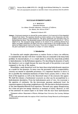
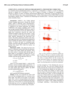
© Copyright 2026