Download Report

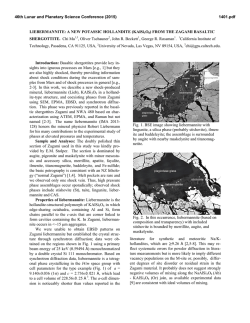
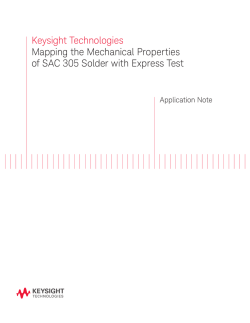
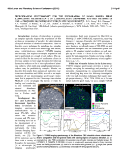
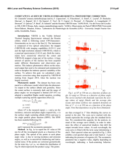
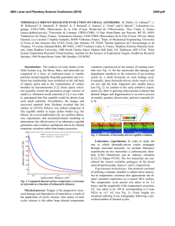
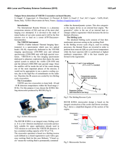
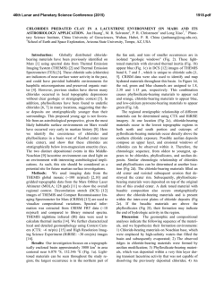
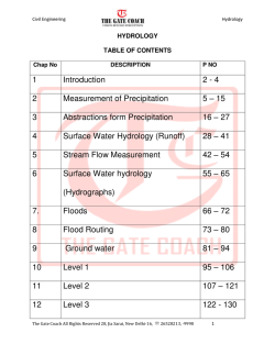
Materials Science and Engineering A 500 (2009) 244–247
Contents lists available at ScienceDirect
Materials Science and Engineering A
journal homepage: www.elsevier.com/locate/msea
Short communication
Hardness based model for determining the kinetics of precipitation
Joy Mittra ∗ , U.D. Kulkarni, G.K. Dey
Materials Science Division, Bhabha Atomic Research Centre, Mumbai 400 085, India
a r t i c l e
i n f o
Article history:
Received 22 April 2008
Received in revised form
12 September 2008
Accepted 17 September 2008
Keywords:
Precipitation
Hardness
Kinetics
Martensitic steel
a b s t r a c t
A theoretical model based on Johnson–Mehl–Avrami (JMA) formalism for determining kinetics and activation energy of a precipitation process is derived from the variation in hardness properties. Effectiveness
of the model for determining the kinetics of ␤-NiAl precipitation in PH13-8Mo steel and for distinguishing
the kinetics between two temperatures is also demonstrated. The activation energy for ␤-precipitation,
244.3 kJ/mol, determined over 808 K to 868 K is in good agreement with that of diffusion of Ni and Al in
␣-iron.
© 2008 Elsevier B.V. All rights reserved.
1. Introduction
Diffusion controlled phase transformation is a function of temperature where, activation energy helps to comprehend the kinetics
of transformation. In the case of diffusion-controlled growth of precipitate through the formation of Guinier–Preston (GP) zone, the
strength of the material usually reaches a peak before falling due
to the loss of coherency [1,2]. In such cases, indirect determination
of activation energies through the measurement of physical properties, such as, strength and hardness becomes easy. In an earlier
attempt by Robino et al. [3], the possibility of using hardness data
in the Johnson–Mehl–Avrami (JMA) model [4,5] was worked out,
assuming the diffusion involving precipitation generates a volume
of soft impingement. As pointed out by Guo, Sha and Wilson [2,6],
JMA formalism represents a real precipitation process and gives a
close approximation in the range of initial stage to high volume
fraction and is seen to be successful in describing the precipitation reaction and austenite reversion process during aging. Hence,
inability of the model by Robino et al. [3] to describe initial stage
of precipitation and questionable conclusion thereof that the JMA
equation might not be suitable to quantify the precipitate fraction
during the aging of PH13-8Mo steel has been discussed by Guo and
Sha [2,6]. Present work re-examines the possibility of using hardness data in the JMA model with signiﬁcant differences form the
earlier approach [3].
∗ Corresponding author. Tel.: +91 22 25590465; fax: +91 22 25505151.
E-mail address: [email protected] (J. Mittra).
0921-5093/$ – see front matter © 2008 Elsevier B.V. All rights reserved.
doi:10.1016/j.msea.2008.09.056
The JMA equation of kinetics expresses the relationship between
volume fraction transformed, x, and the time of transformation, t,
in the following form.
x = 1 − e−kt
n
(1)
Where, n and k are constants by which the kinetics are characterized. The equation may also be written in the following linear
form.
log ln
1
= log k + n log t
(1 − x)
(2)
To incorporate hardness data, we assume that the volume fraction of precipitates, x, is with respect to that of maximum hardness
(HF ) and is related to the hardness via ﬂow properties of the material
in the following manner [3,7].
If H is the difference in hardness, then, H∝x2/3 . If Ht is
the hardness at any time t and H0 is the hardness at t = 0, then,
H = Ht − H0 or, x∝(Ht − H0 )3/2 . It is now expressed in the following
equation form.
x = C0 + C1 (Ht − H0 )3/2
(3)
where, C0 and C1 are constants. To ﬁnd out the constants following
conditions may be set; when Ht = HF , x = 1 and when Ht = H0 , x = 0.
So, C1 = (HF − H0 )−3/2 and C0 = 0. Hence, x = (Ht − H0 )3/2 /(HF − H0 )3/2
is obtained. If x is substituted in Eq. (2), the following expression is
obtained
log ln
(HF − H0 )3/2
(HF − H0 )3/2 − (Ht − H0 )3/2
= log k + n log t
(4)
J. Mittra et al. / Materials Science and Engineering A 500 (2009) 244–247
245
Hence, plotting the left hand term of Eq. (4) against log t, values
of n and k can be determined.
To ﬁnd out the activation energy, Q, of the diffusion controlled
precipitation process, Eq. (1) is differentiated with respect to t and
the rate of a fraction transformed, dx/dt, is found out.
dx
n
= nkt n−1 e−kt
dt
(5)
Where, time for a particular fraction transformed is derived from
Eq. (1), t = {(ln(1 − x)−1 )/k}1/n . When this is replaced in Eq. (5), dx/dt
for a particular fraction transformed is obtained.
If T is absolute temperature, then Arrhenius type rate equation
is written in the following form, A = dx/dt = A0 exp(−Q/8.314T). Or in
the linear form, ln A = ln A0 − Q/8.314T. Hence, Q (J/mol) is calculated
from the slope of the ln (dx/dt) vs. 1/T plot.
Similar to earlier attempt [3], in this case too, ␤-NiAl precipitation in the PH13-8Mo steel has been chosen to evaluate the above
model. In this steel, the ordering of ␤-NiAl precipitate, which is
responsible for high strength of the alloy, is fast and is difﬁcult to
suppress by conventional heat-treatment. However, the precipitate
is highly resistant to overaging, which ensures stability of the alloy
in a long term application [8].
Work by Guo et al. [9], using Position Sensitive Atom Probe
(PoSAP) in wrought PH13-8Mo alloy has indicated that the process of ␤ precipitation consists of following steps. At ﬁrst, solute
rich cluster or Guinier–Preston zone appears in the matrix, which
gradually transforms into ﬁnely distributed transition phase coherent with the matrix, which further coarsens to become incoherent
precipitates of equilibrium composition. The mechanical properties
obtained from hardness measurements and tensile tests indicate
changes in the properties during the early stages of aging. In the
case of aging at a rather low temperature (783 K), precipitations
are detected after 40 min of aging and are of irregular plate morphology. While, in the case of aging at a higher temperature (868 K),
precipitates are detected early after 4 min and are of a needle like
morphology. During the initial stages of aging, precipitates remain
undetected and off stoichiometry, having signiﬁcant amounts of Fe
and Cr atoms in them. Even at this early stage they increase strength
and hardness signiﬁcantly, a behavior similar to that of PH17-4
alloy. The hardening effects observed during early stages of aging
are attributed to the GP zone formation involving redistribution of
Ni and Al [9].
Apart from lacking in clarity, earlier attempt [3] to study the
kinetics of precipitation also appears to lack justiﬁcation in the
consideration of cast variety of PH13-8Mo steel as well as in the
consideration of Rockwell hardness values. Regarding the former
consideration, the wrought variety appears to be superior in terms
of homogenous structure, absence of ␦-ferrite [10] and presence of
less amount of retained austenite [10,11] and as a result of these it
can achieve higher hardness compared to the cast variety.
Regarding the consideration of a hardness scale for establishing
the kinetics [3], as seen in Fig. 1, Vicker’s scale appears to maintain
a more linear relationship with the tensile strength than Rockwell’s
scale. Since, hardness data are incorporated in the model via ﬂow
properties, consideration of Vicker’s scale for the kinetics study is
justiﬁed.
Fig. 1. General trend of Vicker’s (HV) and Rockwell (RC) hardness values with tensile
strength in the region of present interest [12].
Table 1
k and n values obtained through the linear ﬁtting of data points of Fig. 3 using Eq.
(4).
T (K)
783
808
840
868
Fitting of all data
Fitting of 180 s and 1800 s data
k
n
k
n
0.0456
0.1331
0.2886
0.3321
0.408
0.2768
0.2145
0.2572
0.0165
0.076
0.2436
0.3324
0.5795
0.3745
0.2450
0.2572
were taken using the Microhardness Tester having an accuracy
of 0.01 ␮m (Model Future Tech Microhardness Tester, Load range
100–1000 g). For hardness measurement, samples were subjected
to a load of 500 gf and a dwell time of 15 s. For each sample, an
average of the hardness values has been determined and the range
has been shown in the plot in terms of error bar.
3. Results
Fig. 2 shows the plot of average hardness data with error bar
corresponding to samples aged at 783 K, 808 K, 840 K and 868 K for
various durations. Plot of Eq. (4) has been generated using hardness
data till maximum hardness values for the four aging temperatures
and are shown in Fig. 3. For each temperature, two sets of ks and
ns have been determined from the data points of Fig. 3. The ﬁrst
set of ks and ns shown in Table 1 are obtained from the linear ﬁtting of all data points in Eq. (2), while the second set of ks and
2. Experimental
To generate the hardness proﬁle at various temperatures of
aging, small pieces of solutionized wrought PH13-8Mo steel were
aged for 180 s, 1800 s, 7200 s and 14400 s at 783 K, 808 K, 840 K and
868 K, respectively. To see the peak in the hardness proﬁle of former two temperatures, samples were aged for durations ranging
up to 86,400 s (24 h). After aging, hardness values of all samples
Fig. 2. Hardness of PH13-8Mo stainless steel after solutionizing and aging at 783 K,
808 K, 840 K and 868 K for various durations.
246
J. Mittra et al. / Materials Science and Engineering A 500 (2009) 244–247
Fig. 3. Avrami plot produced from the hardness data.
Fig. 4. Fit of x vs. t using 2 analysis for 783 K, 808 K, 840 K and 868 K till maximum
hardness is shown above. 2 values along with k and n values are also tabulated
there. Smooth line plots of the same are shown in the inset, and the lines are drawn
at x (0.5, 0.6, 0.7, 0.8 and 0.9) for determining activation energies.
ns shown in the last column of Table 1 are obtained from that of
ﬁrst two points, corresponding to 180 s and 1800 s. These ks and
ns are only the initial approximation used in the 2 analysis of the
results. Fitting of x vs. t, using 2 method has been shown in Fig. 4
and the experimental data are superimposed on the plot. The inset
of Fig. 4 is the line plot of itself that reveals the trend of x vs. t. This
clearly indicates an out of trend nature of kinetics at 783 K compared to higher temperatures. Plot in the inset also shows lines,
which are drawn at x = 0.5, 0.6, 0.7, 0.8 and 0.9, respectively, to calculate various times taken to transform x at various temperatures.
Rates of transformation for various fractions transformed at every
temperature of aging, which have been derived using Eq. (5) are
given in Table 2. These data, which are based upon 2 method are
depicted in Fig. 5a for determining Qs. However, similar data have
been determined from the kinetics using Eq. (2) and are depicted in
Fig. 5b. As in the case of Fig. 4, in Fig. 5 too the data corresponding to
Fig. 5. Semi-ln plot of rate of transformation and 1/T is derived in (a) using 2 analysis and in (b) using ks and ns from logarithmic plot as per Eq. (2). In both the ﬁgures
best linear ﬁt is obtained separately, including and excluding the data from 783 K
and Q values measured are given in Table 3.
Table 3
Q values derived from Fig. 5a and b, excluding and including data from 783 K.
x
0.5
0.6
0.7
0.8
0.9
Q from 2 analysis
Q from log–log plot (Eq. (2))
808–868 K
All data
808–868 K
All data
233.9
239.1
244.3
249.7
256.5
182.6
166.8
151.5
135.1
115
294
284.9
276
266.5
254.7
230.3
200.3
171.1
140
101.5
783 K deviate from the trend of other temperatures. Hence, activation energies for different x mentioned above have been calculated,
including and excluding the data of 783 K and are shown in Fig. 5a
(Table 3).
Table 2
Time required for the completion of fraction x, (t|x ) and the rate of reaction, dx/dt thereof are calculated using the k and n values obtained through 2 analysis.
(K−1 )
T (K)
1
T
783
808
840
868
1.277 × 10−3
1.238 × 10−3
1.191 × 10−3
1.152 × 10−3
t|x=0.5 (s)
709.7
381.5
99.4
29.2
dx
dt
0.5
2.0227E−4
2.5445E−4
9.718E−4
2.82E−3
t|x=0.6 (s)
1392.2
1033.4
270.6
69.1
dx
dt
0.6
1.0904E−4
9.9343E−5
3.77523E−4
1.16E−3
t|x=0.7 (s)
2691.5
2739.3
720.9
160.3
dx
dt
0.7
5.5584E−5
3.6933E−5
1.3965E−4
4.5701E−4
t|x=0.8 (s)
5424.1
7721.1
2042.3
392.2
dx
dt
0.8
2.4580E−5
1.1677E−5
4.3931E−5
1.5324E−4
t|x=0.9 (s)
12878.0
27732.3
7381.5
1183.1
dx
dt
0.9
7.406E−6
2.3256E−6
8.6947E−6
3.2809E−5
J. Mittra et al. / Materials Science and Engineering A 500 (2009) 244–247
4. Discussion
Study of the kinetics of ␤-NiAl precipitation is carried out at
standard heat-treatment temperatures. Aging at higher than 868 K
is not considered due to the possibility of signiﬁcant amount of ␣
to ␥ transformation, which essentially involves diffusion of carbon
atoms.
It is known from the literature that the process of ␤-nucleation
in PH13-8Mo steel is fast. Hence, a low hardness value of the solution quenched sample, RC20.5 (VHN 240.8), may be attributed to
the suppression of the initiation of ␤-NiAl precipitation, enforced
by the fast quenching, as compared to that of RC30, reported in the
literature [3]. It is important to note here that the linear axes are
used in Fig. 3 and not a log–log one, as used in the earlier work [3], to
ﬁnd out k and n with the help of Eq. (4), since, the intercept for determining the k, can only be obtained in a linear–linear plot. However,
obtaining k and n of Eq. (1) through 2 analysis appears better, since,
goodness of ﬁt, R2 , of 2 analysis of the present data, are better than
that of linear ﬁtting of Eq. (4). Also, ﬁtting of both minimum and
maximum hardness values are shown in the 2 method, whereas,
number of data points from a particular aging temperature reduces
by these two points when Eq. (4) is used.
While, Fig. 4 depicts the scatter in experimental data, which are
superimposed on the data obtained through 2 analysis, nature of
the kinetics may actually be visualized in a smooth plot of Eq. (1), as
shown in the inset. It becomes easy to identify here that the trend
of 783 K is different from that of 808 K, 840 K and 868 K. This is in
support of the PoSAP study reported in the literature [9], where
precipitates at 783 K are found to be of irregular plate morphology, whereas, precipitates at 868 K are of needle like morphology.
As stated earlier, dx/dt, the slope of x vs. t plot is to be used for
determining activation energy and not the ‘1/t’ that is used in the
earlier work [3]. Table 2 shows that the time required for the completion of fraction 0.7 transformed, 160 s, is minimum for 868 K
aging and is close to the minimum aging time, 180 s, set during
experimentation. Hence, there is a minimum extrapolation from
experimentation to the modeled value to determine the activation
energy for the precipitation at 0.7 fraction-transformed. However,
if extrapolation is allowed on the basis of Avrami’s model, then it
is possible to obtain the activation energy, more towards the initiation of precipitation. Hence, the time taken for the completion of
fraction 0.5 for 868 K appears to be 29.2 s.
However, here it should be emphasized that the fraction transformed refers to that of maximum hardness and hence related to
the state of precipitate. And at the maximum hardness, precipitate
may typically be in a coherent to semi-coherent state. Since, NiAl
precipitation in PH13-8Mo is resistant to aging, it appears to be
suitable for the study of precipitation using JMA model.
Process of evaluating activation energies through 2 analysis
and Eq. (4), as shown in Fig. 5, support the superiority of the former
method. As identiﬁed in Fig. 4, in this case too, data corresponding
247
to 783 K stands out from the rest. Since, the concept of activation energy is applicable when a particular process is valid over
a range of temperature, it is intuitive to select 808–868 K temperatures for the calculation of activation energy and hence, data from
783 K is not considered for calculating activation energy. An equivalent comparison of the activation energies, which are obtained
from Fig. 5a and b, respectively, shows that the Qs, based on 2
method and in the range of 808–868 K temperature show minimum scatter. The difference from highest Q, at x = 0.9, to lowest
Q, at x = 0.5 is 22.6 kJ/mol and is seen to vary linearly with x. The
activation energy of NiAl precipitation at 0.7 fraction transformed,
244.3 kJ/mol, appears closely matching with that of diffusion
of Ni and Al in ␣-iron, which are 235 kJ/mol and 246 kJ/mol,
respectively.
5. Conclusion
Suppression of ␤-NiAl precipitation in PH13-8Mo by fast cooling results in a low hardness of the alloy. In this work, a systematic
method for determining kinetics of precipitation and activation
energy from hardness data has been established using JMA’s model.
Obtaining constants of the JMA equation through ﬁtting of data
directly using reduced 2 method appears better than ﬁtting linearized JMA equation. The present methodology also helps in
comparing the nature of kinetics at different temperatures and
in determining activation energy more accurately. The activation
energy of the NiAl precipitation appears very close to that of diffusion of Ni and Al in ␣-iron.
Acknowledgements
Authors would like to thank Mr. Abhishek Chauhan and Mr.
Somesh Dutt for various helps during experimentation. Authors are
also grateful to Dr. A.K. Suri, Director, Materials Group for extending
various facilities to carry out the present work.
References
[1] A.J. Ardell, Mater. Trans. A 16A (1985) 2131–2165.
[2] Z. Guo, W. Sha, Mater. Trans. 43 (2002) 1273–1282.
[3] C.V. Robino, P.W. Hochanadel, G.R. Edwards, M.J. Cieslak, Metall. Mater. Trans.
A 25A (1994) 697–704.
[4] W.A. Jhonson, R.F. Mehl, Trans. Am. Inst. Min. (Metall) Engrs. 135 (1939) 416.
[5] M.J. Avrami, Chem. Phys. 8 (1940) 212–224.
[6] Z. Guo, W. Sha, E.A. Wilson, Mater. Sci. Technol. 18 (2002) 377–382.
[7] J.W. Martin, Precipitation Hardening, 2nd Ed., Butterworth-Heinemann, Oxford,
1998, p. 91.
[8] V. Seetharaman, M. Sundararaman, R. Krishnan, Mater. Sci. Eng. 47 (1981)
1–11.
[9] Z. Guo, W. Sha, D. Vaumousse, Acta Mater. 51 (2003) 101–116.
[10] P.W. Hochanadel, C.V. Robino, G.R. Edwards, M.J. Cieslak, Metall. Mater. Trans.
A 25A (1994) 789–798.
[11] J. Mittra, G.K. Dey, D. Sen, A.K. Patra, S. Mazumder, P.K. De, Scr. Mater. 51 (2004)
349–353.
[12] Internet: http://www.wargamer.org/GVA/background/hardness4.html.