1. Art and Diseño

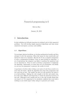
A modified hybrid genetic algorithm for solving
nonlinear optimal control problems
R. Ghanbari1 , S. Nezhadhosein2∗ , A. heydari3
1
Department of Applied Mathematics, Faculty of Mathematical science, Ferdowsi University of Mashhad, Mashhad, Iran
2,3 Department of Applied Mathematics, Payame Noor University, Tehran, Iran
*Corresponding author E-mail:s [email protected]
Abstract
Here, a two-phase algorithm is proposed for solving bounded continuous-time nonlinear optimal control problems (NOCP).
In each phase of the algorithm, a modified hybrid genetic algorithm (MHGA) is applied, which performs a local search on
offsprings. In first phase, a random initial population of control input values in time nodes is constructed. Next, MHGA starts
with this population. After phase 1, to achieve more accurate solutions, the number of time nodes is increased. The values
of the associated new control inputs are estimated by Linear interpolation (LI) or Spline interpolation (SI), using the curves
obtained from the phase 1. In addition, to maintain the diversity in the population, some additional individuals are added
randomly. Next, in the second phase, MHGA restarts with the new population constructed by above procedure and tries to
improve the obtained solutions at the end of phase 1. We implement our proposed algorithm on 20 well-known benchmark
and real world problems, then the results are compared with some recently proposed algorithms. Moreover, two statistical
approaches are considered for the comparison of the LI and SI methods and investigation of sensitivity analysis for the MHGA
parameters.
Keywords: Optimal control problem, Hybrid genetic algorithm, Spline interpolation.
1.
Introduction
NOCPs are dynamic optimization problems with many applications in industrial processes such as airplane, robotic arm, bioprocess system, biomedicine, electric power systems, plasma physics and etc., [7].
High-quality solutions and the less required computational time are main issues for solving NOCPs. The numerical methods,
direct [21] or indirect [32], usually have two main deficiencies, less accuracy and convergence to a local solution. In direct
methods, the quality of solution depends on discretization resolution. Since these methods, using control parametrization,
convert the continuous problem to discrete problem, they have less accuracy. However, the adaptive strategies [8, 29] can
overcome these defects, but they may be trapped by a local optimal, yet. In indirect approaches, the problem, through the use
of the Pontryagins minimum principle (PMP), is converted into a two-boundary value problem (TBVP) that can be solved by
numerical methods such as shooting method [31]. These methods need the good initial guesses that lie within the domain of
convergence. Therefore, the numerical methods, usually are not suitable for solving NOCPs, especially for large-scale and
multimodal models.
Metaheuristics as the global optimization methods can overcome these problems, but they usually need more computational
time, though they don’t really need good initial guesses and deterministic rules. Several researchers used metaheuristics to
solve optimal control problems. For instance, Michalewicz et al. [25] applied floating-point Genetic algorithms (GA) to solve
discrete time optimal control problems, Yamashita and Shima [38] used the classical GAs to solve the free final time optimal
control problems with terminal constraints. Abo-Hammour et al. [1] used continuous GA for solving NOCPs. Moreover,
the other usages of GA for optimal control problems can be found in [31, 30]. Lopez-Cruz et al. [11] applied Differential
Evolution (DE) algorithms for solving the multimodal optimal control problems. Recently, Ghosh et al. [19] developed an
ecologically inspired optimization technique, called Invasive Weed Optimization (IWO), for solving optimal control problems.
The other well-known metaheuristic algorithms used for solving NOCPs are Genetic Programming (GP) [22], Particle Swarm
Optimization (PSO) [4, 3], Ant Colony Optimization (ACO) [35] and DE [23, 37].
To increase the quality of solutions and decrease the running time, hybrid methods were introduced, which used a local
search in the implementation of a population-based metaheuristics, [6]. Modares and Naghibi-Sistani [26] proposed a hybrid
algorithm by integrating an improved PSO with successive quadratic programming (SQP) for solving NOCPs. Recently, Sun
2
et al. [33] proposed a hybrid improved GA, which used Simplex method (SM) to perform a local search, for solving NOCPs
and applied it for chemical processes.
Based on the success of the hybrid methods for solving NOCPs, mentioned above, we here use a modified hybrid Genetic
algorithm (MHGA), which combines GA with SQP, see [9], as a local search. SQP is an iterative algorithm for solving
nonlinear programming (NLP) problems, which uses gradient information. It can moreover be used for solving NOCPs, see
[34, 20, 14]. For decreasing the running time in the early generations (iterations) of MHGA, a less number of iterations for
SQP was used and then, when the promising region of search space was found, we increase the number of iterations of SQP,
gradually.
To perform MHGA for solving an NOCP, the time interval is uniformly divided by using a constant number of time nodes.
Next, in each of these time nodes, the control variable is approximated by a scaler vector of control input values. Thus, an
infinite dimensional NOCP is changed to a finite dimensional NLP. Now, we encounter two conflict situations: the quality of
the global solution and the needed computational time. In other words, when the number of time nodes is increased, then we
expect the quality of the global solution is also increased, but we know that in this situation the computational time is increased
dramatically. In other situation, if we consider less number of time nodes, then the computational time is decreased but we
may find a poor local solution. To conquer these problems, MHGA performs in two phases. In the first phase (exploration
phase), to decrease the computational time and to find a promising regions of search space, MHGA uses a less number of time
nodes. After phase 1, to increase the quality of solutions obtained from phase 1, the number of time nodes is increased. Using
the population obtained in the phase 1, the values of the new control inputs are estimated by Linear or Spline interpolations.
Next, in the second phase (exploitation phase), MHGA uses the solutions constructed by the above procedure, as an initial
population.
The paper is organized as follows: in Section 2, the formulation of the problem is introduced. In Section 3, the proposed
MHGA is presented. In Section 4, we introduce our algorithm for solving NOCP. In Section 5, we provide 20 numerical
benchmark examples, to compare the proposed algorithm with the other recently proposed algorithms. In Section 6, we
consider two statistical approaches for the comparison of the LI and SI methods and investigation of sensitivity analysis of the
algorithm parameters. The impact of SQP, as local search, in the proposed algorithm is surveyed in Section 7. We conclude
in Section 8.
2.
Formulation of problem
The bounded continuous-time NOCP is considered as finding the control input u(t) ∈ Rm , over the planning horizon [t0 ,t f ],
that minimizes the cost functional:
J = ϕ (x(t f ),t f ) +
∫ tf
g(x(t), u(t),t)dt
(1)
t0
subject to :
x(t)
˙ = f (x(t), u(t),t),
(2)
c(x, u,t) = 0,
d(x, u,t) ≤ 0,
(3)
(4)
ψ (x(t f ),t f ) = 0,
x(t0 ) = x0 .
(5)
(6)
where x(t) ∈ Rn denotes the state vector for the system and x0 ∈ Rn is the initial state. The functions f : Rn × Rm × R → Rn , g :
Rn × Rm × R → R, c : Rn × Rm × R → Rnc , d : Rn × Rm × R → Rnd , ψ : Rn × R → Rnψ and ϕ : Rn × R → R are assumed
to be sufficiently smooth on appropriate open sets. The cost function (1) must be minimized subject to dynamic (2), control
and state equality constraints (3) and control and state inequality constraints (4), the final state constraints (5) and the initial
condition (6). A special case of the NOCPs is the linear quadratic regulator (LQR) problem where the dynamic equations are
linear and the objective function is a quadratic function of x and u. The minimum time problems, tracking problem, terminal
control problem and minimum energy are another special cases of NOCPs.
3.
Modified hybrid genetic algorithm
In this Section, first MHGA, as a subprocedure for the main algorithm, is introduced. To perform MHGA, the control variables
are discretized. Next, NOCP is changed into a finite dimensional NLP, see [15, 33]. Now, we can imply a GA to find the
global solution of the corresponding NLP. In the following, we introduce GA operators.
3
3.1.
Underlying GA
GAs introduced by Holland in 1975, are heuristics and probabilistic methods [13]. These algorithms start with an initial
population of solutions. This population is evaluated by using genetic operators that include selection, crossover and mutation.
Here, in MHGA, the underling GA has the following steps:
Initialization: The time interval is divided into Nt − 1 subintervals using time nodes t0 , . . . ,tNt −1 and then the control input
values are computed (or selected randomly). This can be done by the following stages:
1. Let t j = t0 + jh, where h =
respectively.
t f −t0
Nt −1 ,
j = 0, 1, . . . , Nt − 1, be time nodes, where t0 and t f are the initial and final times,
2. The corresponding control input value at each time node t j is an m × 1 vector, u j , which can be calculated randomly,
with the following components.
ui j = u j (i) = ule f t (i) + (uright (i) − ule f t (i)).ri j ,
i = 1, 2, . . . , m,
j = 0, 1, . . . , Nt − 1
(7)
where ri j is a random number in [0, 1] with a uniform distribution and ulelt , uright ∈ Rm are the lower and the upper bound
vectors of control input values, which can be given by the problem’s definition or the user (e.g. see the NOCPs no. 6 and
t −1
5 in Appendix A, respectively). So, each individual of the population is an m × Nt matrix as U = (ui j )m×Nt = [u j ]Nj=0
.
Next, we let U (k) = (ui j )m×Nt , k = 1, 2, . . . , N p as k-th individual of the population, which Np is the size of the population.
Evaluation: For each control input matrix, U (k) , k = 1, 2, . . . , N p , the corresponding state variable is an n × Nt matrix, X (k) ,
and it can be computed by the forth Runge-Kutta method on dynamic system (2) with the initial condition (6), approximately.
˜ If NOCP includes equality or
Then, the performance index, J(U (k) ), is approximated by a numerical method (denoted by J).
inequality constraints (3) or (4), then we add some penalty terms to the corresponding fitness value of the solution. Finally,
we assign I(U (k) ) to U (k) as the fitness value as follows:
nd Nt −1
nc Nt −1
l=1 j=0
h=1 j=0
I(U (k) ) = J˜+ ∑
nψ
∑ M1l max{0, dl (x j , u j ,t j )} + ∑ ∑ M2h c2h (x j , u j ,t j ) + ∑ M3p ψ p2 (xNt −1 ,tNt −1 )
(8)
i=p
where M1 = [M11 , . . . , M1nd ]T , M2 = [M21 , . . . , M2nc ]T and M3 = [M31 , . . . , M3nψ ]T are big numbers, as the penalty parameters
, ch (., .), h = 1, 2, . . . , nc , dl (., .), l = 1, 2, . . . , nd , and ψ p (., .), p = 1, 2, . . . , nψ are defined in (3), (4) and (5), respectively.
Selection: To select two parents, we use a tournament selection [13]. It can be applied for parallel GA. The tournament
operator apply competition among the some individuals, and the best of them is selected for next generation. At first we select
a specified number of individuals from population, randomly. This number is tournament selection parameter, which is denote
by Ntour . The tournament algorithm is given in Algorithm 1.
Crossover: When two parents U (1) and U (2) are selected, we use the following stages to construct an offspring:
Algorithm 1 Tournament algorithm
{Initialization} Input the the size of tournament, Ntour and select Ntour individuals from population, randomly. Let ki , i =
1, 2, . . . , Ntour be the indexes of them.
repeat
if Ntour = 2 then
if I(U k1 ) < I(U k2 ) then
Let k = k1 .
else
Let k = k2 .
end if
end if
Perform Tournament algorithm with size Ntour
2 with output k1 .
Ntour
Perform Tournament algorithm with size 2 with output k2 .
until k1 ̸= k2
Return the k-th individual of population.
1. Select the following numbers
λ1 ∈ [0, 1], λ2 ∈ [−λmax , 0], λ3 ∈ [1, 1 + λmax ]
randomly, where λmax is a random number in [0, 1].
(9)
4
2. Let
o f k = λkU (1) + (1 − λk )U (2) ,
k = 1, 2, 3
(10)
where λk , k = 1, 2, 3 is defined in (9). For i = 1 . . . m and j = 1, . . . , Nt , if (o f k )i j > uright,i , then let (o f k )i j = uright,i and
if (o f k )i j < ule f t,i , then let (o f k )i j = ule f t,i .
3. Let o f = o f ∗ , where o f ∗ is the best o f k , k = 1, 2, 3 constructed by (10).
Mutation: We apply a perturbation on each component of the offspring as follows:
(o f )i j = (o f )i j + ri j .α ,
i = 1, 2, . . . , m, j = 1, 2, . . . , Nt
(11)
where ri j is selected randomly in {−1, 1} and α is a random number, with a uniform distribution in [0, 1]. If (o f )i j > uright,i ,
then let (o f )i j = uright,i and if (o f )i j < ule f t,i , then let (o f )i j = ule f t,i .
Replacement: Here, in the underling GA, we use a traditional replacement strategy. The replacement is done, if the new
offspring has two properties: first, it is better than the worst person in the population, I(o f ) < max1≤i≤Np I(U (i) ) , second, it
isn’t very similar to a person in the population, i.e. for each i = 1, . . . , N p , at least one of the following conditions satisfied:
|I(o f ) − I(U (i) )| > ε´ ,
(12)
∥o f −U ∥ > ε´
(13)
(i)
where ε´ is the machine epsilon.
Termination conditions: Underlying GA is terminated when at least one of the following conditions is occurred:
1. The maximum number of generations, Ng , is reached .
2. Over a specified number of generations, Ni , we don’t have any improvement (the best individual is not changed) or the
two-norm, or error, of final state constraints will reached to a small number as the desired precision, ε , i.e.
φ f = ∥ψ ∥2 < ε
(14)
where ψ = [ψ1 , ψ2 , . . . , ψnψ ]T is the vector of final state constraints, defined in (5).
3.2.
SQP
The fitness value in (8), can be viewed as a nonlinear objective function with the decision variable as u = [u0 , u1 , . . . , uNt −1 ].
This cost function with upper and lower bounds of input signals construct a finite dimensional NLP problem as following
min
I(u) = I(u0 , u1 , . . . , uNt −1 )
s.t
ule f t ≤ u j ≤ uright ,
j = 0, 1, . . . , Nt − 1
(15)
SQP algorithm [9, 28] is performed on the NLP (15), using u¯0 = o f , constructed in (11), as the initial solution when the
maximum number of iteration is sqpmaxiter.
SQP, is an effective and iterative algorithm for the numerical solution of the constrained NLP problem. This technique is
based on finding a solution to the system of nonlinear equations that arise from the first-order necessary conditions for an
extremum of the NLP problem. Using an initial solution of NLP, u¯k , k = 0, 1, . . ., a sequence of solutions as u¯k+1 = u¯k + d k
is constructed, which d k is the optimal solution of the constructed quadratic programming (QP) that approximates NLP in
the iteration k based on u¯k , as the search direction in the line search procedure. For the NLP (15), the principal idea is the
formulation of a QP subproblem based on a quadratic approximation of the Lagrangian function as L(u, λ ) = I(u) + λ T h(u),
where the vector λ is Lagrangian multiplier and h(u) return the vector of, inequality constraints evaluated at u. The QP is
obtained by linearizing the nonlinear functions as following:
1
min d T H(u¯k )d + ∇I(u¯k )T d
2
∇h(u¯k )T d + h(u¯k ) ≤ 0
(16)
Similar to [15], here a finite difference approximation is applied to compute the gradient of the cost function and the constraints, with the following components
I(...u j + δ ...) − I(u)
∂I
=
,
∂uj
δ
j = 0, 1, . . . , Nt − 1
(17)
5
where δ is the double precision of machine. So, the gradient vector is ∇I = [ ∂∂uI , . . . , ∂ u∂ I ]T . Also, at each major iteration
0
Nt −1
a positive definite quasi-Newton approximation of the Hessian of the Lagrangian function, H, is calculated using the BFGS
method [28], where λi , i = 1, ..., m, is an estimate of the Lagrange multipliers. The general procedure for SQP, for NLP (15),
is as following
1. Given an initial solution u¯0 . Let k = 0.
2. Construct the QP subproblem (16), based on u¯0 , using the approximations of the gradient and the Hessian of the the
Lagrangian function.
3. Compute the new point as u¯k+1 = u¯k + d k , where d k is the optimal solution of the current QP.
4. Let k=k+1 and go to step 2.
Here, in MHGA, SQP is used as the local search, and we use the maximum number of iterations as the main criterion for
stopping SQP. In other words, we terminate SQP when it converges either to local solution or the maximum number of SQP’s
iterations is reached.
3.3.
MHGA
In MHGA, GA uses a local search method to improve solutions. Here, we use SQP as a local search. Using SQP as a local
search in the hybrid metaheuristic is common, for example, see [26].
MHGA can be seen as a multi start local search where initial solutions are constructed by GA. From another perspective,
MHGA can be seen as a GA that the quality of its population is intensified by SQP. In the beginning of MHGA, a less
number of iterations for SQP was used. Then, when the promising regions of search space were found by GA operators, we
increase the number of iterations of SQP gradually. Using this approach, we may decrease the needed running time (in [6] the
philosophy of this approach is discussed.
Finally, we give our modified MHGA, to find the global solution, by the flowchart in Fig 1.
4.
Proposed algorithm
Here, we give a new algorithm, which is a direct approach, based on MHGA, for solving NOCPs. The proposed algorithm has
two main phases. In the first phase, we perform MHGA with a completely random initial population constructed by (7). In
the first phase, to find the promising regions of the search space, in a less running time, we use a few numbers of time nodes.
In addition, to have a faster MHGA, the size of the population in the first phase is usually less than the size of the population
in the second phase.
After phase 1, to maintain the property of individuals in the last population of the phase 1 and to increase the accurately of
solutions, we add some additional time nodes. When the number of time nodes is increased, it is estimated that the quality of
solution obtained by numerical methods (e.g. Runge-Kutta and Simpson) is increased. Thus, we increase time nodes from Nt1
in the phase 1 to Nt2 in the phase 2. The corresponding control input values of the new time nodes are added to individuals.
To use the information of the obtained solutions from phase 1 in the construction of the initial population of the phase 2, we
use either Linear or Spline interpolation to estimate the value of the control inputs in the new time nodes in each individual of
the last population of phase 1. Moreover, to maintain the diversity in the initial population of the phase 2, we add new random
individuals to the population using (7). In the second phase, MHGA starts with this population and new value of parameters.
Finally, the proposed algorithm is given in Algorithm 2.
Algorithm 2 The proposed algorithm
{Initialization} Input the desired precision, ε , in (14), the penalty parameters, Mi , i = 1, 2, 3, in (8), the bounds of control
input values in (7), ule f t and uright .
{Phase 1} Perform MHGA with a random population and Nt1 , N p1 , Ni1 , Ng1 , Pm1 and sqpmaxiter1 .
{Construction of the initial population of the phase 2} Increase time nodes uniformly to Nt2 and estimate the corresponding control input values of the new time nodes in each individual obtained from phase 1, using either Linear or Spline
interpolation.
Create N p2 − N p1 new different individuals with Nt2 time nodes, randomly.
{Phase 2} Perform MHGA with the constructed population and Nt2 , N p2 , Ni2 , Ng2 , Pm2 and sqpmaxiter2 .
6
Fig 1: Flowchart of the MHGA algorithm.
5.
.
Initialization
Input Nt , N p , Ni , Ng , Pm ,
.
sqpmaxiter,
ε , Mi , i = 1, 2, 3 and
an initial population.
.
.
Evaluation
Evaluate. the fitness of each individual, using (8).
.
.
Local search
.
(Section 3.2)
.
Return
The best individual in
the final population
.
as an approximate
of the global solution of NOCP.
.
Stopping
.
conditions?
.
.
Selection
.
(Algorithm 1)
sqpmaxiter
=
.
sqpmaxiter + 1
.
Crossover
.
(using equation (10))
Replacement
(using. equations (12), (13))
.
Mutation
.
(using equation (11))
Local search
.
(Section 3.2)
Numerical experiments
In this Section, to investigate the efficiency of the proposed algorithm, 20 well-known and real world NOCPs, as benchmark
problems, are considered which are presented in terms of eqns (1)-(6) in Appendix A. These NOCPs are selected with single
control signal and multi control signals, which will be demonstrated in a general manner.
The numerical behaviour of algorithms can be studied from two view of points, the relative error of the performance index
and the status of the final state constraints. Let J be the obtained performance index by an algorithm, φ f , defined in (14), be
the error of final state constraints, and J ∗ be the best obtained solution among all implementations, or the exact solution (when
exists). Now the relative error of J, EJ , of the algorithm can be defined as
EJ = |
J − J∗
|
J∗
(18)
To more accurate study, we now define a new criterion, called factor, to compare the algorithms as follows:
Kψ = EJ + φ f ,
(19)
7
Note that Kψ shows the summation of two important errors. Thus, based on Kψ we can study the behaviour of the algorithms
on the quality and feasibility of given solutions, simultaneously.
To solve any NOCP described in Appendix A, we must know the algorithm’s parameters including: MHGA’s parameters;
including Nt , N p , Ni , Ng , Pm and sqpmaxiter, in both phases in Algorithn 2, and the problem’s parameters including ε , in
(14), Mi , i = 1, 2, 3, in (8), ule f t and uright , in (7). To estimate the best value of the algorithm’s parameters, we ran the proposed
algorithm with different values of parameters and then select the best. However, the sensitivity of MHGA parameters are
studied in the next Section. In both of phases of Algorithm 2, in MHGA, we let sqpmaxiteri = 4 and Pmi = 0.8 , for i = 1, 2.
Also, we consider Ng1 = Ng2 , Ni1 = Ni2 , N p1 = 9 and N p2 = 12. The other MHGA parameters are given in the associated
subsection and the problem’s parameters in Table 2. For each NOCP, 12 different runs were done and the best results are
reported in Table 1, which the best value of each column is seen in the bold.
The reported numerical results of the proposed algorithm, for each NOCP, include the value of performance index, J, the
relative error of J, EJ , defined in (18), the required computational time, Time, the norm of final state constraints, φ f , defined
in (14) and the factor, Kψ , defined in (19).
The algorithm was implemented in Matlab R2011a environment on a Notebook with Windows 7 Ultimate, CPU 2.53 GHz
and 4.00 GB RAM. Also, to implement SQP in our proposed algorithm, we used ‘fmincon’ in Matlab when the ‘Algorithm’
was set to ‘SQP’. Moreover, we use the composite Simpson’s method [5] to approximate integrations.
Remark 5.1 We use the following abbreviations to show the used interpolation method in our proposed algorithm:
1. LI: linear interpolation.
2. SI: spline interpolation.
For comparing the numerical results of the proposed algorithm two subsections are considered, comparison with some metaheuristic algorithms, in Section 5.1, and comparison with some numerical methods, in Section 5.2. We give more details of
these comparisons in the following subsections.
5.1.
Comparison with metaheuristic algorithms
The numerical results for the NOCPs no. 1-3, in Appendix A, are compared with a continuous GA, CGA, as a metaheuristic,
proposed in [1], which gave better solutions than shooting method and gradient algorithm, from the indirect methods category
[21, 10], and SUMT from the direct methods category [15]. For NOCPs no. 4 and 5, the results are compared with another
metaheuristic, which is a hybrid improved PSO, called IPSO, proposed in [26].
5.1.1.
VDP problem [1]
The first NOCP in Appendix A is Van Der Pol Problem, VDP, which has two state variables and one control variable. VDP
problem has a final state constraint, which is ψ = x1 (t f ) − x2 (t f ) + 1 = 0. The results of the proposed algorithm with the
MHGA’s parameters as Nt1 = 31, Nt2 = 71, Ng = 300 and Ni = 200, are reported in Table 1. From Table 1, it is obvious that
the numerical results of LI and SI methods are more accurate than CGA, with less amount of Kψ .
5.1.2.
CRP problem [1]
The second NOCP in Appendix A is Chemical Reactor Problem, CRP, which has two state variables and one control variable.
The results of the proposed algorithm, with the MHGA’s parameters as Nt1 = 31, Nt2 = 71, Ng = 300 and Ni = 200, are shown
in the second row of Table 1. CRP problem has two final state constraints, ψ = [x1 , x2 ]T . Although, from Table 1, the norm
of final state constraints, φ f , for the CGA, equals φ ∗f = 7.57 × 10−10 , is less than φ f ’s of LI and SI methods, which equals
1.15 × 10−9 and 5.99 × 10−9 , respectively, but the performance index, the relative error of J and the factor of the proposed
algorithm is better, and so the proposed algorithm is more robust than CGA.
5.1.3.
FFRP problem [1]
The third NOCP in Appendix A is Free Floating Robot Problem, FFRP, which has six state variables and four control variables.
FFRP has been solved by CGA and the proposed algorithm, with the MHGA’s parameters as Nt1 = 31, Nt2 = 71, Ng = 300
and Ni = 200. This problem has six final state constraints, ψ = [x1 − 4, x2 , x3 − 4, x4 , x5 , x6 ]T . The numerical results are shown
in Table 1. The values of J, EJ , φ f and Kψ for LI and SI methods, separately, are less than CGA. Therefore, the proposed
algorithm can achieve much better quality solutions than the CGA, with reasonable computational time.
8
5.1.4.
MSNIC problem [26]
For the forth NOCP in Appendix A, which is a Mathematical System with Nonlinear Inequality Constraint, NSNIC, the
numerical results are compared with IPSO. MSNIC contains an inequality constraint, d(x,t) = x2 (t) + 0.5 − 8(t − 0.5)2 ≤ 0.
The problem solved by several numerical methods as [20, 24]. From [26], IPSO method could achieved more accurate results
than mentioned numerical methods. Also, MSNIC can be solved by the proposed algorithm, with the MHGA’s parameters as
Nt1 = 31, Nt2 = 91, Ng = 100 and Ni = 60. From the forth row of Table 1, the absolute error of J, EJ , for LI and SI methods
equal 0 and 5.89 × 10−4 , respectively, which are less than IPSO’s, (0.0165).
Sub-plots (a) and (b) in Fig 2, show the graphs of the convergence rate for the performance index and the inequality constraint,
respect to the number of iteration, respectively.
0.205
0
0.2
−0.5
Inequality constraint
Performance index
0.195
0.19
0.185
−1
−1.5
0.18
−2
0.175
0.17
0
5
10
15
20
25
Iter
30
35
40
45
50
−2.5
0
0.1
0.2
0.3
0.4
0.5 0.6
Time
0.7
0.8
0.9
1
Fig 2: Graphical results of MSNIC problem using SI method: (a) convergence rate of the performance index, (b) the inequality constraint,
d(x,t) ≤ 0, respect to the number of iteration.
5.1.5.
CSTCR problem [26]
The fifth NOCP in Appendix A is a model of a nonlinear Continuous Stirred-tank Chemical Reactor, CSTCR. It has two state
variables x1 (t) and x2 (t), as the deviation from the steady-state temperature and concentration, and one control variable u(t),
which represent the effect of the flow rate of cooling fluid on chemical reactor. The objective is to maintain the temperature
and concentration close to steady-state values without expending large amount of control effort. Also, this is a benchmark
problem in the handbook of test problems in local and global optimization [16], which is a multimodal optimal control
problem [2]. It involves two different local minima. The values of the performance indexes, for these solutions, equal
0.244 and 0.133. Similarly to the MSNIC, the numerical results of the proposed algorithm, with the MHGA’s parameters as
Nt1 = 31, Nt2 = 51, Ng = 100 and Ni = 50, are compared with IPSO. From Table 1, the performance index, J, for LI and SI
methods are equal to J ∗ = 0.1120 which is less than IPSO’s (0.1355).
5.2.
Comparison with numerical methods
For NOCPs no. 6-20, the comparison are done with some numerical methods. Unfortunately, for these methods, usually, the
final state constraints and the required computational time are not reported, which are shown with NR in Table 1, but these
values are reported for both LI and SI methods in Table 1. For all NOCPs , in this Section, the MHGA’s parameters are
considered as Nt1 = 31, Nt2 = 51, Ng = 100, Ni = 50 , with the problem parameters in Table 2.
5.2.1.
Compared with B´ezier [18]
The NOCP no. 6, in Appendix A, has exact solution, which has an inequality constraint as d(x1 ,t) = −6 − x1 (t) ≤ 0. The
exact value of performance index equals J ∗ = −5.5285 [36]. This problem has been solved by a numerical method proposed
in [18], called B´ezier. From sixth row of Table 1, the absolute error of the LI and SI methods equal 0.0177, which is less than
the B´ezier’s, 0.0251.
9
Fig 3, shows the graphs of the convergence rate of the performance index, sub-plot (a), and inequality constraint, sub-plot (b),
respect to the number of iteration, using SI method.
−5.343
0
−5.344
−1
−5.345
−2
Inequality constraint
Performance index
−5.346
−5.347
−5.348
−5.349
−3
−4
−5
−5.35
−6
−5.351
−7
−5.352
−5.353
2
4
6
8
Iter
10
12
14
−8
0
0.5
1
1.5
Time
2
2.5
3
Fig 3: Graphical results for NOCP no. 6 using SI method: (a) convergence rate for the performance index, (b) the inequality constraint,
d(x1 ,t) ≤ 0, respect to the number of iteration.
5.2.2.
Compared with HPM [12]
For NOCP no. 7 in Appendix A, which is a constraint nonlinear model, the numerical results of the proposed algorithm are
compared with HPM, proposed in [12]. This NOCP has a final state constraint as ψ = x − 0.5 = 0. From [12], the norm of
final state constraint for HPM equals 4.2 × 10−6 , however, this criterion for the LI and SI methods equals 2.35 × 10−9 and
φ ∗f = 2.82 × 10−10 , respectively. From Table 1, it is obvious that the obtained values of the performance index, the norm of
final state constraint and Kψ for the SI method are more accurate than LI than HPM methods.
5.2.3.
Compared with SQP and SUMT [15]
For the NOCPs no. 8-20, in Appendix A, the numerical results of LI and SI methods are compared with two numerical methods
contain: SQP and SUMT, proposed in [15]. Among these NOCPs, only two problems no. 8 and 18 are unconstrained, and the
others have at least one constraint, final state constraint or inequality constraint. All of these NOCPs solved by the proposed
algorithm, with the problem parameters in Table 2, and their results are summarized in Table 1. Because the final state
constraints, in these methods, are not reported, we let φ f = 0 to calculate the factor Kψ .
Also, the Figs 4-16, in Appendix B, show the graphical results for NOCPs no. 8-20, using SI method. These Figs contain the
convergence rates of performance index, the final state constraints, and the inequality constraint (for NOCPs no. 9 and 10),
for constraint NOCPs, with respect to the number of iteration.
Table 1: The best numerical results in 12 different runs of the SI and LI methods for NOCPs in Appendix A.
Problem
VDP
CRP
FFRP
Algorithm
CGA
LI
SI
CGA
LI
SI
CGA
LI
SI
J
1.7404
1.5949
1.5950
1.63 × 10−2
1.27 × 10−2
1.27 × 10−2
83.63
35.96
35.99
EJ
0.0912
0
6.27 × 10−5
0.2835
0
0
1.3256
0
8.34 × 10−4
φf
2.67 × 10−11
1.08 × 10−13
9.99 × 10−14
7.57 × 10−10
1.15 × 10−9
5.99 × 10−9
4.65 × 10−3
1.22 × 10−5
9.01 × 10−6
Kψ
Time
0.0912
501.28
1.08 × 10−13
282.82
6.27 × 10−5
239.14
0.2835
501.28
1.15 × 10−9
171.94
5.99 × 10−9
124.05
1.3302
1413
1.22 × 10−5
1268.58
8.43 × 10−4
1343.40
Continued on next page
10
Problem
MSNIC
CSTCR
No . 6
No . 7
No . 8
No . 9
No . 10
No . 11
No . 12
No . 13
No . 14
No . 15
No . 16
No . 17
No . 18
Algorithm
IPSO
LI
SI
IPSO
LI
SI
B´ezier
LI
SI
HPM
LI
SI
SQP
SUMT
LI
SI
SQP
SUMT
LI
SI
SQP
SUMT
LI
SI
SQP
SUMT
LI
SI
SQP
SUMT
LI
SI
SQP
SUMT
LI
SI
SQP
SUMT
LI
SI
SQP
SUMT
LI
SI
SQP
SUMT
LI
SI
SQP
SUMT
LI
SI
SQP
Table 1 – Continued from previous page
J
EJ
φf
0.1727
0.0165
—
0.1699
0
—
0.1700
5.89 × 10−4
—
0.1355
0.2098
—
0.1120
0
—
0.1120
0
—
−5.3898
0.0251
—
−5.4309
0.0177
—
−5.4309
0.0177
—
0.2353
0.1677
4.20 × 10−6
0.2015
0
2.35 × 10−9
0.2015
0
2.82 × 10−10
6.36 × 10−6
2.20 × 109
—
−6
5.15 × 10
1.78 × 109
—
2.89 × 10−15
0
—
3.64 × 10−15
0.2595
—
1.7950
0.0873
—
1.7980
0.0891
—
1.6509
0
—
1.6509
0
—
0.2163
0.3964
—
0.1703
0.0994
—
0.1549
0
—
0.1549
0
—
3.25
0.1648
0
3.25
0.1648
0
2.7901
0
1.62 × 10−9
2.7901
0
5.86 × 10−10
−3
−0.2490
4.0 × 10
0
−0.2490
4.0 × 10−3
0
−0.2500
0
2.85 × 10−8
−0.2500
0
3.90 × 10−10
1.68 × 10−2
0.1748
0
1.67 × 10−2
0.1678
0
−2
1.43 × 10
0
1.18 × 10−9
−2
−3
1.44 × 10
7.0 × 10
6.32 × 10−9
3.7220
0.0961
0
3.7700
0.1103
0
3.3956
0
7.86 × 10−7
3.3965
2.65 × 10−4
2.76 × 10−6
−3
1.03 × 10
4.3368
0
9.29 × 10−4
3.8135
0
1.93 × 10−4
0
8.10 × 10−10
1.94 × 10−4 5.20 × 10−3
1.64 × 10−9
2.2120
0.0753
0
2.2080
0.0734
0
2.0571
0
3.94 × 10−12
2.0571
0
5.60 × 10−13
−5
−8.8690
2.25 × 10
0
−8.8690
2.25 × 10−5
0
−8.8692
0
1.45 × 10−10
−8.8692
0
2.79 × 10−10
0.0368
0.1288
—
Kψ
Time
—
126.26
—
138.82
—
138.68
—
31.34
—
103.58
—
106.73
—
NRa
—
138.38
—
107.34
0.1677
NR
2.35 × 10−9
213.92
2.82 × 10−10
206.96
—
NR
—
NR
—
72.82
—
68.68
—
NR
—
NR
—
639.10
—
595.0
—
NR
—
NR
—
625.70
—
676.62
0.1648
NR
0.1648
NR
1.62 × 10−9
147.78
5.86 × 10−10
219.46
4.0 × 10−3
NR
4.0 × 10−3
NR
2.85 × 10−8
547.71
3.90 × 10−10
545.48
0.1748
NR
0.1678
NR
−9
1.18 × 10
425.99
7.0 × 10−3
490.27
0.0961
NR
0.1103
NR
7.86 × 10−7
1041.24
2.67 × 10−4
1151.44
4.3368
NR
3.8135
NR
8.10 × 10−10
333.54
5.20 × 10−3
340.14
0.0753
NR
0.0734
NR
3.94 × 10−12
469.82
5.60 × 10−13
704.23
2.25 × 10−5
NR
2.25 × 10−5
NR
1.45 × 10−10
321.83
2.79 × 10−10
309.59
—
NR
Continued on next page
11
Table 2: The problem parameters for NOCPs in Appendix A.
Problem no.
Parameters 1
2
3
4
5
6
7 8 9 10
ule f t
−0.5 −1.5 −15 −20 0 −2 0 −2 −1 −20
uright
2
2
10 20 5
2
1 2 1 20
Mi
103 102 70 1 —
1
— 102 — 102
ε
10−12 10−10 10−3 — — — — — — 10−9
Problem no.
Parameters 11 12 13 14 15 16 17 18 19 20
ule f t
−5 −1 −2 −π −1 −3 −30 −1 −15 −15
π
1
3
30 1 10 10
uright
5
1
2
Mi
10 102 — 102 102 102 — 10 70 10−3
ε
10−9 10−11 10−11 — 10−10 10−10 10−10 — 10−3 10−4
Problem
No . 19
No . 20
a
Algorithm
SUMT
LI
SI
SQP
SUMT
LI
SI
SQP
SUMT
LI
SI
Table 1 – Continued from previous page
J
EJ
φf
0.0386
0.1840
—
0.0326
0
—
0.0326
0
—
0.3439
4.9293
0
0.3428
4.9103
0
0.0689
0.1879
4.10 × 10−3
0.0580
0
4.05 × 10−4
77.52
1.2554
0
76.83
1.2353
0
34.3716
2.32 × 10−5
2.25 × 10−4
34.3708
0
1.57 × 10−4
Kψ
—
—
—
4.9293
4.9103
0.1919
4.05 × 10−4
1.2554
1.2353
2.48 × 10−4
1.57 × 10−4
Time
NR
551.63
606.71
NR
NR
1645.09
1787.83
NR
NR
815.19
804.20
Not Reported.
Table 1 shows that the proposed algorithm, LI and SI methods, was 100 percent successful in point of views the performance index, J, and the factor, Kψ , numerically. So, the proposed algorithm provides robust solutions with respect to the other
mentioned, numerical or metaheuristic, methods. To compare J in LI and SI methods, in 35 percent of NOCPs, LI is more
accurate than SI, in 10 percent SI is more accurate than LI and in 55 percent are same. In point of view the final conditions,
65 percent of NOCPs in Appendix A have final state constraints. In all of them φ f in the proposed algorithm is improved,
except CRP problem, however the factor of the proposed algorithm is the best, yet. In 54 percent of these NOCPs, LI is better
performance and in 46 percent SI is better. Also, in point of the running time, Time, LI is same as SI, i.e. in 50 percent of
NOCPs LI and in 50 percent SI is better than another. So, the proposed algorithm could provide very suitable solutions, in a
reasonable computational time. Also, for more accurate comparison of LI and SI methods a statistical approach will done in
next Section.
To compare with CGA, the mean of relative error of J, EJ , for CGA, LI and SI methods, in NOCPs 1-3, equal 0.5668, 0
and 2.98 × 10−4 , respectively. Also the mean for the error of the final state constraints, φ f , are 1.6 × 10−3 , 4.07 × 10−6 and
3.01 × 10−6 , respectively, and for Kψ , these values equal 0.5883, 4.07 × 10−6 and 3.02 × 10−4 . Thus, we can say that the
feasibility of the solutions given by the proposed algorithm and CGA are competitive.
From Table 1, to compare with numerical methods, SQP and SUMT, in NOCPs 8-20, the mean of EJ for LI, SI, SQP and
SUMT equals 0.0145, 0.0209, 1.69 × 108 and 1.36 × 108 , respectively. Also, the mean for the error of final state constraints,
for these NOCPs, equal 3.34 × 10−4 , 4.41 × 10−5 0 and 0, respectively. For Kψ , these values are 0.0213, 0.0014, 1.2263 and
1.1644. Therefore, the performance index, J, and the factor, Kψ , for the LI and SI methods are more accurate than SQP and
SUMT. So the proposed algorithm gave more better solution in comparison with the numerical methods.
Therefore, based on this numerical study, we can conclude that the proposed algorithm outperform well-known numerical
method. Since, the algorithms were not implemented on the same PC, the computational times of them are not competitive.
Therefore, we didn’t give the computational times in bold in Table 1.
12
6.
Sensitivity analysis and comparing LI and SI
In this Section, two statistical analysis, based on the one-way analysis of variance (ANOVA), used for investigating the
sensitivity of MHGA parameters, and Mann-Whitney, applied comparing LI and SI methods, are done, by the statistical
software IBM SPSS version 21.
6.1.
Sensitivity analysis
In order to survey the sensitivity of the MHGA parameters from the proposed algorithm, the VDP problem is selected,
for example. The influence of these parameters are investigated for this NOCP on the dependent outputs consist of the
performance index, J , the relative error of J, EJ , the required computational time, Time, the error of final state constraints, φ f
and the factor, Kψ . The independent parameters are consist of the number of time nodes in both two phases, Nt1 and Nt2 , the
size of population in both two phases, Np1 and N p2 , the maximum number of generations without improvement, Ni , and the
maximum number of generations, Ng . Because the mutation implementation probability, Pm , has a less influence in numerical
results, it is not considered. Also sqpmaxiter is changed in each iteration of the proposed algorithm, so it is not considered
too.
At first, we selected at least four constant value for each of parameters and then in each pose, 35 different runs were made,
independently. The statistical analysis is done based on ANOVA. The descriptive statistics, which contains the number of
different runs (N), the mean of each output in N different runs, (Mean), standard deviation, (S.d), maximum, (Max) and
minimum, (Min), of each output, could be achieved. Among of the MHGA parameters, we present the descriptive statistics
of the ANOVA, only for the Nt1 parameter, which is reported in Table 3.
Table 4, summarized the statistical data, contain the test statistics (F) and p-values, of ANOVA tests. Sensitivity analysis for
each parameter, separately, are done based on this Table, as following:
Nt1 : From Table 4, the significant level, or p-value, for Kψ is equal to 0.279, which is greater than 0.05. So, from ANOVA,
Nt1 parameter has no significant effect on the factor Kψ . With similar analysis, this parameter has no effect on the other
outputs, except required computational time, Time, because its p-value is equal to 0, which is less than 0.05, i.e. this
output sensitive to the parameter Nt1 .
Nt2 : From the second row of Table 4, the outputs J, EJ , Kψ and Time are sensitive to the parameter Nt2 , and the only output
φ f is independent.
N p1 : From the third row of Table 4, only the computational required time, Time, is sensitive, because the its p-value is equal
to 0.006, which is less than 0.05, and the other outputs, contain J, EJ , φ f , Kψ , are independent.
N p2 : From the forth row of Table 4, the output φ f is independent respect to the parameter Np2 , but other outputs, contain
J, EJ , Time, Kϕ are sensitive to this parameter.
Ng : From the fifth row of Table 4, the outputs J, EJ and Kψ are independent to the parameter Ng , and other outputs, contain
φ f and Time are sensitive respect to this parameter.
Ni : The sensitivity analysis is similar to N p1 .
From above cases, it is obvious that all parameters can be effect on the required computational time, except Ng . Moreover,
intuitions shows the norm of final state constraints, φ f is independent output with respect to all parameters, i.e. any of the
parameters could not effect on this output and it is not sensitive with respect to any of the MHGA parameters.
6.2.
Comparison of LI and SI
To compare the efficiency of the LI and SI methods, for NOCPs in Appendix A, we used the Mann-Whitney nonparametric
statistical test [27]. Using the nonparametric statistical tests for comparing the performance of several algorithms presented
in [17]. For this purpose, At first, 15 different runs, for each of NOCP were made. Table 5, shows the mean of numerical
results, separately. Here, we apply the fix MHGA parameters as N p1 = 9, Np2 = 12, Nt1 = 31, Nt2 = 91, Ng = 100 and
Ni = 50 with the previous problem parameters in Table 2. Comparison criterions contain: J, φ f , Kψ and Time. The results of
Mann-Whitney test are shown in Tables 6-9. From Table 6, since Z = 0 > Z0.01 = −2.34, then the average relative error of the
LI and SI methods are same with the significant level 0.01. In other words, with probability 99%, we can say that LI and SI
methods have same effectiveness form the perspective of error for J. Similarly , the results of Tables 7-9 indicate that LI and
SI methods, from the perspective of errors for φ f , Time and Kψ , have same behaviour.
13
Table 3: Descriptive statistics for the sensitivity analysis of Nt1 , for VDP problem.
Output
J
φf
Time
EJ
Kψ
Nt1
11
21
31
41
Total
11
21
31
41
Total
11
21
31
41
Total
11
21
31
41
Total
11
21
31
41
Total
N
35
35
35
35
140
35
35
35
35
140
35
35
35
35
140
35
35
35
35
140
35
35
35
35
140
Mean
1.5333
1.5328
1.5329
1.5455
1.5357
2.81 × 10−8
4.67 × 10−8
1.63 × 10−8
8.17 × 10−8
4.26 × 10−8
89.7838
109.8147
116.3591
144.8290
114.2131
0.0031
0.0028
0.0029
0.0111
0.0047
0.0031
0.0027
0.0029
0.0111
0.0047
S.d
0.0069
0.0097
0.0076
0.0607
0.0294
9.52 × 10−8
2.35 × 10−7
4.91 × 10−8
2.85 × 10−7
1.91 × 10−7
27.2081
46.0264
30.0227
39.3091
41.0891
0.0045
0.0064
0.0050
0.0397
0.0192
0.0045
0.0064
0.0050
0.0397
0.0192
Min
1.5286
1.5285
1.5285
1.5285
1.5285
1 × 10−12
1 × 10−12
1 × 10−12
1 × 10−12
1 × 10−12
45.6614
60.4192
77.2673
81.0425
45.6615
0
0
0
0
0
4.75 × 10−9
5.50 × 10−10
1.54 × 10−13
1.93 × 10−10
1.54 × 10−13
Max
1.5598
1.5849
1.5699
1.8449
1.8449
4.52 × 10−7
1.41 × 10−6
2.21 × 10−7
1.26 × 10−6
1.41 × 10−6
155.4394
284.0310
179.5103
284.9514
284.9514
0.0204
0.0369
0.0271
0.2070
0.2070
0.0204
0.0369
0.0271
0.2070
0.2070
Table 4: Summary statistical data of ANOVA test for the parameters, Nt1 , Nt2 , N p1 , N p2 , Ng , Ni .
Test statistic (F)
p-value
Parameters
Nt1
Nt2
N p1
N p2
Ng
Ni
Nt1
Nt2
N p1
N p2
Ng
Ni
J
1.294
1105.72
1.945
2.740
3.541
0.495
0.280
0
0.125
0.021
0.009
0.739
EJ
1.296
3.93
1.835
2.478
3.591
0.309
0.279
0.005
0.143
0.034
0.008
0.819
φf
0.624
0.868
1.271
1.011
0.491
0.301
0.601
0.489
0.286
0.413
0.743
0.877
Time
10.79
59.39
4.317
23.02
0.890
5.849
0
0
0.006
0
0.472
0
Kψ
1.296
3.93
1.835
2.478
3.591
1.046
0.279
0.005
0.143
0.034
0.008
0.386
14
Table 5: The mean of numerical results of 15 different runs for NOCPs in Appendix A, using LI and SI methods.
LI
SI
Kψ
Kψ
Problem
J
φf
Time
J
φf
Time
VDP
1.5977 1.57 × 10−9 1.70 × 10−3 177.20 1.6002 6.67 × 10−8 3.26 × 10−3 157.57
CRP
0.0126 3.07 × 10−8 3.07 × 10−8 197.14 0.0119 1.61 × 10−8 1.61 × 10−8 195.32
FFPP
47.74
8.05 × 10−5 0.3277 1332.80 53.51
5.92 × 10−5 0.4868 1379.89
MSNIC 0.1702
—
—
136.78 0.1703
—
—
140.92
CSTCR 0.1120
—
—
173.85 0.1120
—
—
176.06
No . 6
−5.4307
—
—
105.41 −5.4308
—
—
103.72
No . 7
0.2015 3.26 × 10−9 6.95 × 10−6 208.07 0.2020 3.13 × 10−9 6.62 × 10−6 210.19
No . 8 6.30 × 10−15
—
—
63.76 1.24 × 10−14
—
—
58.37
No . 9
1.6512
—
—
592.39 1.6512
—
—
581.25
No . 10
0.1550
—
—
631.53 0.1550
—
—
655.97
No . 11
2.9701 2.70 × 10−9 2.72 × 10−7 228.60 2.9701 3.37 × 10−9 8.11 × 10−7 232.76
No . 12 −0.2499 2.01 × 10−8 4.64 × 10−5 547.18 −0.2499 1.15 × 10−9 8.27 × 10−5 527.65
No . 13
0.0147 1.15 × 10−8 0.0252 577.97 0.0151 1.39 × 10−8 0.0472 660.98
No . 14
3.4761 6.72 × 10−6 0.0237 1045.85 3.4290 7.57 × 10−6 9.50 × 10−3 1087.67
No . 15 1.95 × 10−4 1.11 × 10−8 5.69 × 10−3 363 1.94 × 10−4 7.04 × 10−9 4.86 × 10−3 365
No . 16
2.0571 1.66 × 10−10 1.66 × 10−10 543.91 2.0571 1.15 × 10−10 1.15 × 10−10 544.31
No . 17 −8.8692 8.03 × 10−8 8.03 × 10−8 227.44 −8.8692 6.61 × 10−8 6.61 × 10−8 232.54
No . 18
0.0326
—
—
659.57 0.0326
—
—
708.97
No . 19 0.11588 6.55 × 10−4 0.6828 1618.13 0.1091 8.84 × 10−4 0.8808 1599.90
No . 20
52.42
0.0176
0.5429 841.65
44.64
4.53 × 10−4 0.3765 868.91
Table 6: Results of Mann-Whitney test on relative errors of the pair (LI,SI) for J.
Method
LI
SI
—
Mean rank
20.50
20.50
—
Sum of ranks
410.0
410.0
—
Test statistics
Mann-Whitney U
Wilcoxon W
Z
Value
200
410
0
Table 7: Results of Mann-Whitney test on relative errors of the pair (LI,SI) for φ f .
Method
LI
SI
—
Mean rank
13.62
13.38
—
Sum of ranks
177
174
—
Test statistics
Mann-Whitney U
Wilcoxon W
Z
Value
83
174
-0.077
Table 8: Results of Mann-Whitney test on relative errors of the pair (LI,SI) for Time.
Method
LI
SI
—
Mean rank
20.25
20.75
—
Sum of ranks
405.0
415.0
—
Test statistics
Mann-Whitney U
Wilcoxon W
Z
Value
195
405
-0.135
Table 9: Results of Mann-Whitney test on relative errors of the pair (LI,SI) for Kψ .
Method
LI
SI
—
Mean rank
13.54
13.46
—
Sum of ranks
176.0
175.0
—
Test statistics
Mann-Whitney U
Wilcoxon W
Z
Value
84
175
-0.026
15
Table 10: The numerical results of the without SQP algorithm, for NOCPs in Appendix A.
7.
J
ϕf
1
1.7296
3.30 × 10−9
2
0.0174
1.35 × 10−5
3
213.80
1.1445
4
0.1702
—
J
ϕf
11
4.8816
1.67 × 10−5
12
−0.1273
4.68 × 10−9
13
0.0153
0.0161
14
4.5727
4.33 × 10−4
Problem no.
5
6
0.1130
−5.2489
—
—
Problem no.
15
16
9.79 × 10−4
2.3182
5.94 × 10−3
1.56 × 10−5
7
0.2390
7.58 × 10−9
8
1.69 × 10−1
—
9
1.8606
—
10
0.2048
—
17
−9.0882
1.64
18
0.0336
—
19
25.13
17.06
20
202.74
2.5283
The impact of SQP
In this section, we investigation the impact of the SQP, on the proposed algorithm. For this purpose, we remove the SQP from
Algorithm 2, as without SQP algorithm. For comparing the numerical results with the previous results, the required running
time in each NOCP is considered fixed, which is the maximum of running time in 12 different runs, were done in Section
5. Also, the all of the parameters for each problem was set as same as Section 5. The numerical results of the without SQP
algorithm is summarized in Table 10. By comparing the results of Table 10 and Table 1, it is obvious that, for all NOCPs in
Appendix A, the obtained values of the performance index and the norm of final state constraint for the proposed algorithm
(Algorithm 2), are more accurate than the without SQP algorithm.
8.
Conclusions
Here, a two-phase algorithm was proposed for solving bounded continuous-time NOCPs. In each phase of the algorithm, a
MHGA was applied, which performed a local search on offsprings. In first phase, a random initial population of control input
values in time nodes was constructed. Next, MHGA started with this population. After phase 1, to achieve more accurate
solutions, the number of time nodes was increased. The values of the associated new control inputs were estimated by Linear
interpolation (LI) or Spline interpolation (SI), using the curves obtained from the phase 1. In addition, to maintain the diversity
in the population, some additional individuals were added randomly. Next, in the second phase, MHGA restarted with the new
population constructed by above procedure and tried to improve the obtained solutions at the end of phase 1. We implemented
our proposed algorithm on 20 well-known benchmark and real world problems, then the results were compared with some
recently proposed algorithms. Moreover, two statistical approaches were considered for the comparison of the LI and SI
methods and investigation of sensitivity analysis for the MHGA parameters.
References
[1] Zaer S. Abo-Hammour, Ali Ghaleb Asasfeh, Adnan M. Al-Smadi, and Othman M. K. Alsmadi, A novel continuous
genetic algorithm for the solution of optimal control problems, Optimal Control Applications and Methods 32 (2011),
no. 4, 414–432.
[2] M.M. Ali, C. Storey, and A. T¨orn, Application of stochastic global optimization algorithms to practical problems, Journal
of Optimization Theory and Applications 95 (1997), no. 3, 545–563 (English).
[3] M. Senthil Arumugam, G. Ramana Murthy, and C. K. Loo, On the optimal control of the steel annealing processes as a
two stage hybrid systems via PSO algorithms, International Journal Bio-Inspired Computing 1 (2009), no. 3, 198–209.
[4] M. Senthil Arumugam and M. V. C. Rao, On the improved performances of the particle swarm optimization algorithms
with adaptive parameters, cross-over operators and root mean square (RMS) variants for computing optimal control of
a class of hybrid systems, Application Soft Computing 8 (2008), no. 1, 324–336.
[5] K. Atkinson and W. Han, Theoretical numerical analysis: A functional analysis framework, Texts in Applied Mathematics, Springer, 2009.
[6] Saman Babaie-Kafaki, Reza Ghanbari, and Nezam Mahdavi-Amiri, Two effective hybrid metaheuristic algorithms for
minimization of multimodal functions, International Journal Computing Mathematics 88 (2011), no. 11, 2415–2428.
[7] John T. Betts, Practical methods for optimal control and estimation using nonlinear programming, Society for Industrial
and Applied Mathematics, 2010.
16
[8] T. Binder, L. Blank, W. Dahmen, and W. Marquardt, Iterative algorithms for multiscale state estimation, part 1: Concepts, Journal of Optimization Theory and Applications 111 (2001), no. 3, 501–527.
[9] J.J.F. Bonnans, J.C. Gilbert, C. Lemar´echal, and C.A. Sagastiz´abal, Numerical optimization: Theoretical and practical
aspects, Springer London, Limited, 2006.
[10] A.E. Bryson, Applied optimal control: Optimization, estimation and control, Halsted Press book’, Taylor & Francis,
1975.
[11] I.L. Lopez Cruz, L.G. Van Willigenburg, and G. Van Straten, Efficient differential evolution algorithms for multimodal
optimal control problems, Applied Soft Computing 3 (2003), no. 2, 97 – 122.
[12] S. Effati and H. Saberi Nik, Solving a class of linear and non-linear optimal control problems by homotopy perturbation
method, IMA Journal of Mathematical Control and Information 28 (2011), no. 4, 539–553.
[13] A.P. Engelbrecht, Computational intelligence: An introduction, Wiley, 2007.
[14] Brian C. Fabien, Numerical solution of constrained optimal control problems with parameters, Applied Mathematics
and Computation 80 (1996), no. 1, 43 – 62.
[15] Brian C. Fabien, Some tools for the direct solution of optimal control problems, Advances Engineering Software 29
(1998), no. 1, 45–61.
[16] C.A. Floudas and P.M. Pardalos, Handbook of test problems in local and global optimization, Nonconvex optimization
and its applications, Kluwer Academic Publishers.
[17] Salvador Garc´ıa, Daniel Molina, Manuel Lozano, and Francisco Herrera, A study on the use of non-parametric tests for
analyzing the evolutionary algorithms behaviour: acase study onthecec2005 special session onreal parameter optimization, Journal of Heuristics 15 (2009), no. 6, 617–644.
[18] F Ghomanjani, M.H Farahi, and M Gachpazan, B´ezier control points method to solve constrained quadratic optimal
control of time varying linear systems , Computational and Applied Mathematics 31 (2012), 433 – 456 (en).
[19] Arnob Ghosh, Swagatam Das, Aritra Chowdhury, and Ritwik Giri, An ecologically inspired direct search method for
solving optimal control problems with ber parameterization, Engineering Applications of Artificial Intelligence 24
(2011), no. 7, 1195 – 1203.
[20] C.J. Goh and K.L. Teo, Control parametrization: A unified approach to optimal control problems with general constraints, Automatica 24 (1988), no. 1, 3 – 18.
[21] Donald E. Kirk, Optimal control theory: An introduction, Dover Publications, 2004.
[22] A. Vincent Antony Kumar and P. Balasubramaniam, Optimal control for linear system using genetic programming,
Optimal Control Applications and Methods 30 (2009), no. 1, 47–60.
[23] Moo Ho Lee, Chonghun Han, and Kun Soo Chang, Dynamic optimization of a continuous polymer reactor using a
modified differential evolution algorithm, Industrial and Engineering Chemistry Research 38 (1999), no. 12, 4825–4831.
[24] Wichaya Mekarapiruk and Rein Luus, Optimal control of inequality state constrained systems, Industrial and Engineering Chemistry Research 36 (1997), no. 5, 1686–1694.
[25] Zbigniew Michalewicz, Cezary Z. Janikow, and Jacek B. Krawczyk, A modified genetic algorithm for optimal control
problems, Computers Mathematics with Applications 23 (1992), no. 12, 83 – 94.
[26] Hamidreza Modares and Mohammad-Bagher Naghibi-Sistani, Solving nonlinear optimal control problems using a hybrid IPSO - SQP algorithm, Engineering Applications of Artificial Intelligence 24 (2011), no. 3, 476 – 484.
[27] D.C. Montgomery, Applied statistics and probability for engineers, John Wiley & Sons Canada, Limited, 1996.
[28] J. Nocedal and S.J. Wright, Numerical optimization, Springer series in operations research and financial engineering,
Springer, 1999.
[29] Martin Schlegel, Klaus Stockmann, Thomas Binder, and Wolfgang Marquardt, Dynamic optimization using adaptive
control vector parameterization, Computers Chemical Engineering 29 (2005), no. 8, 1731 – 1751.
17
[30] X. H. Shi, L. M. Wan, H. P. Lee, X. W. Yang, L. M. Wang, and Y. C. Liang, An improved genetic algorithm with
variable population-size and a PSO-GA based hybrid evolutionary algorithm, Machine Learning and Cybernetics, 2003
International Conference on, vol. 3, 2003, pp. 1735–1740.
[31] Y. C. Sim, S. B. Leng, and V. Subramaniam, A combined genetic algorithms-shooting method approach to solving
optimal control problems, International Journal of Systems Science 31 (2000), no. 1, 83–89.
[32] B. Srinivasan, S. Palanki, and D. Bonvin, Dynamic optimization of batch processes: I. characterization of the nominal
solution, Computers Chemical Engineering 27 (2003), no. 1, 1 – 26.
[33] Fan SUN, Wenli DU, Rongbin QI, Feng QIAN, and Weimin ZHONG, A hybrid improved genetic algorithm and its application in dynamic optimization problems of chemical processes, Chinese Journal of Chemical Engineering 21 (2013),
no. 2, 144 – 154.
[34] K.L. Teo, C.J. Goh, and K.H. Wong, A unified computational approach to optimal control problems, Pitman monographs
and surveys in pure and applied mathematics, Longman Scientific and Technical, 1991.
[35] Jelmer Marinus van Ast, Robert Babuˇska, and Bart De Schutter, Novel ant colony optimization approach to optimal
control, International Journal of Intelligent Computing and Cybernetics 2 (2009), no. 3, 414–434.
[36] Jacques Vlassenbroeck, A chebyshev polynomial method for optimal control with state constraints, Automatica 24
(1988), no. 4, 499 – 506.
[37] Feng-Sheng Wang and Ji-Pyng Chiou, Optimal control and optimal time location problems of differential-algebraic
systems by differential evolution, Industrial and Engineering Chemistry Research 36 (1997), no. 12, 5348–5357.
[38] Yuh Yamashita and Masasuke Shima, Numerical computational method using genetic algorithm for the optimal control
problem with terminal constraints and free parameters, Nonlinear Analysis: Theory, Methods Applications 30 (1997),
no. 4, 2285 – 2290.
Appendix A
The following problems are presented using notation given in eqns (1)-(6).
1. (VDP) [1] g = 12 (x12 + x22 + u2 ), t0 = 0,t f = 5, f = [x2 , −x2 + (1 − x12 )x2 + u]T , x0 = [1, 0]T , ψ = x1 − x2 + 1.
1
2. (CRP) [1] g = 12 (x12 + x22 + 0.1u2 ), t0 = 0,t f = 0.78, f = [x1 − 2(x1 + 0.25) + (x2 + 0.5) exp( x25x
) − (x1 + 0.25)u, 0.5 −
1 +2
1
x2 − (x2 + 0.5)exp( x25x
)]T , x0 = [0.05, 0]T , ψ = [x1 , x2 ]T .
1 +2
1
1
3. (FFRP) [1] g = 12 (u21 + u22 + u23 + u24 ), t0 = 0, t f = 5, f = [x2 , 10
((u1 + u2 ) cos x5 − (u2 + u4 ) sin x5 ), x4 , 10
((u1 +
5
T
T
u3 ) sin x5 + (u2 + u4 ) cos x5 ), x6 , 12 ((u1 + u3 ) − (u2 + u4 ))] , x0 = [0, 0, 0, 0, 0, 0] , ψ = [x1 − 4, x2 , x3 − 4, x4 , x5 , x6 ]T .
4. (MSNIC) [26] ϕ = x3 , t0 = 0, t f = 1, f = [x2 , −x2 + u, x12 + x22 + 0.005u2 ]T , d = [−(u − 20)(u + 20), x2 + 0.5 − 8(t −
0.5)2 ]T , x0 = [0, −1, 0]T .
1
5. (CSTCR) [26] g = x12 + x22 + 0.1u2 , t0 = 0, t f = 0.78, f = [−(2 + u(x1 + 0.25) + (x2 + 0.5) exp( x25x
), 0.5 − x2 − (x2 +
1 +2
1
)]T , x0 = [0.09, 0.09]T .
0.5)exp( x25x
1 +2
6. [18] g = 2x1 , t0 = 0, t f = 3, f = [x2 , u]T , d = [−(2 + u)(2 − u), −(6 + x1 )]T , x0 = [2, 0]T .
7. [12]g = u2 ,t0 = 0,t f = 1, f = 12 x2 sin x + u, x0 = 0, ψ = x − 0.5.
8. [15] g = x2 cos2 u, t0 = 0, t f = π , f = sin u2 , x0 = π2 .
9. [15] g = 12 (x12 + x22 + u2 ), t0 = 0, t f = 5, f = [x2 , −x1 + (1 − x12 )x2 + u]T , d = −(x2 + 0.25), x0 = [1, 0]T .
10. [15] g = x12 + x22 + 0.005u2 , t0 = 0, t f = 1, f = [x2 , −x2 + u]T , d = [−(20 + u)(20 − u), −(8(t − 0.5)(t − 0.5) − 0.5 −
x2 )]T , x0 = [0, −1]T .
11. [15] g = 12 u2 , t0 = 0, t f = 2, f = [x2 , u]T , x0 = [1, 1]T , ψ = [x1 , x2 ]T .
18
12. [15] g = −x2 , t0 = 0, t f = 1, f = [x2 , u]T , d = −(1 − u)(1 + u), x0 = [0, 0]T , ψ = x2 .
1
13. [15] g = 21 (x12 + x22 + 0.1u2 ), t0 = 0, t f = 0.78, f = [−2(x1 + 0.25) + (x2 + 0.5)exp( x25x
) − (x1 + 0.25)u, 0.5 − x2 −
1 +2
1
(x2 + 0.5)exp( x25x
)]T , x0 = [0.05, 0]T , ψ = [x1 , x2 ]T .
1 +2
14. [15] g = 12 u2 , t0 = 0, t f = 10, f = [cos u − x2 , sin u]T , d = −(π + u)(π − u), x0 = [3.66, −1.86]T , ψ = [x1 , x2 ]T .
1
15. [15] g = 12 (x12 + x22 ), t0 = 0, t f = 0.78, f = [−2(x1 + 0.25) + (x2 + 0.5)exp( x25x
) − (x1 + 0.25)u, 0.5 − x2 − (x2 +
1 +2
1
0.5)exp( x25x
)]T , d = −(1 − u)(1 + u), x0 = [0.05, 0]T , ψ = [x1 , x2 ]T .
1 +2
16. [15] ϕ = x3 , t0 = 0, t f = 1, f = [x2 , u, 21 u2 ]T , d = x1 − 1.9, x0 = [0, 0, 0]T , ψ = [x1 , x2 + 1]T .
17. [15] ϕ = −x3 , t0 = 0, t f = 5, f = [x2 , −2 + xu3 , −0.01u]T , d = −(30 − u)(30 + u), x0 = [10, −2, 10]T , ψ = [x1 , x2 ]T .
18. [15] ϕ = (x1 − 1)2 + x22 + x32 , g = 21 u2 , t0 = 0, t f = 5, f = [x3 cos u, x3 sin u, sin u]T , x0 = [0, 0, 0]T .
19. [15] g = 4.5(x32 + x62 ) + 0.5(u21 + u22 ), t0 = 0, t f = 1, f = [9x4 , 9x5 , 9x6 , 9(u1 + 17.25x3 ), 9u2 , − x92 (u1 − 27.075x3 +
2x5 x6 )]T , x0 = [0, 22, 0, 0, −1, 0]T , ψ = [x1 − 10, x2 − 14, x3 , x4 − 2.5, x5 , x6 ]T .
20. [15] similar to problem 3 with ψ = [x1 − 4, x2 , x3 − 4, x4 , x5 − π4 , x6 ]T .
Appendix B
Figs 4-16 show the graphical results of NOCPs no. 8-20 in Appendix A, using SI method. For unconstrained NOCPs, no. 8
and 18, only the graph of convergent rate of performance index is shown, Figs 4 and 14. For constraint NOCPs, NOCPs no.
11-17 and no. 19-20, with final state constraint, the graphs of convergent rates of performance index and the error of final
state constraint are shown, Figs 7-13 and 15-16. For the constraint NOCPs with inequality constraints, NOCPs no. 9 and 10,
the graphs of convergent rate of performance index and inequality constraint are shown, Figs 5 and 6.
−5.343
0
−5.344
−1
−5.345
−2
Inequality constraint
Performance index
−5.346
−5.347
−5.348
−5.349
−3
−4
−5
−5.35
−6
−5.351
−7
−5.352
−5.353
2
4
6
8
Iter
10
12
14
−8
0
0.5
1
1.5
Time
2
2.5
3
Fig 4: Convergence rate for the performance index of SI method for NOCP no. 8.
19
0.25
0.2
Inequality constraint
Performance index
1.85
1.8
1.75
1.7
0.15
0.1
0.05
1.65
5
10
15
20
0
25
0
0.5
1
1.5
2
2.5
Time
Iter
3
3.5
4
4.5
5
Fig 5: (a) Convergence rate for the performance index and (b) the inequality constraint of SI method, for NOCP no. 9.
0
0.205
0.2
−0.5
Inequality constraint
Performance index
0.195
0.19
0.185
0.18
0.175
−1
−1.5
0.17
−2
0.165
0.16
0.155
5
10
15
20
25
Iter
30
35
40
45
50
−2.5
0
0.1
0.2
0.3
0.4
0.5
Time
0.6
0.7
0.8
0.9
1
Fig 6: (a) Convergence rate of the performance index and (b) the inequality constraint for SI method, for NOCP no. 10.
−5
−0.225
1.6
x 10
1.4
−0.23
Final condition
Performance index
1.2
−0.235
−0.24
1
0.8
0.6
0.4
−0.245
0.2
−0.25
5
10
15
Iter
20
25
0
1
1.5
2
2.5
3
3.5
Iter
4
4.5
5
5.5
6
Fig 7: (a) Convergence rates of the performance index and (b) the error of final state constraint for SI method, for NOCP no. 11.
20
Fig 8: (a) Convergence rates of the performance index and (b) the error of final state constraint for SI method, for NOCP no. 12.
−3
0.7
9
x 10
8
0.6
7
6
Final condition
Performance index
0.5
0.4
0.3
5
4
3
0.2
2
0.1
0
1
1
2
3
4
5
6
7
8
9
0
10
1
2
3
4
5
Iter
6
7
8
9
10
Iter
Fig 9: (a) Convergence rates of the performance index and (b) the error of final state constraint for SI method, for NOCP no. 13.
9
0.6
8.5
0.5
8
0.4
7
Final condition
Performance index
7.5
6.5
6
5.5
0.3
0.2
5
4.5
0.1
4
3.5
5
10
15
Iter
20
25
30
0
1
2
3
4
5
6
7
8
9
10
Iter
Fig 10: (a) Convergence rates of the performance index and (b) the error of final state constraint for SI method, for NOCP no. 14.
21
4.5
0.099
4
0.0985
3.5
x 10
3
0.098
Final condition
Performance index
−3
0.0995
0.0975
0.097
2.5
2
1.5
0.0965
1
0.096
0.5
0.0955
5
10
15
20
25
Iter
30
35
40
45
0
50
2
4
6
8
10
12
14
16
18
20
Iter
Fig 11: (a) Convergence rates of the performance index and (b) the error of final state constraint for SI method, for NOCP no. 15.
−3
2.7
6
2.6
5
4
Final condition
Performance index
2.5
x 10
2.4
2.3
3
2
2.2
1
2.1
5
10
15
20
0
25
1
2
3
4
Iter
5
6
7
8
Iter
Fig 12: (a) Convergence rates of the performance index and (b) the error of final state constraint for SI method, for NOCP no. 16.
1
−8.78
0.9
−8.79
0.8
−8.8
0.7
Final condition
Performance index
−3
−8.77
−8.81
−8.82
−8.83
0.6
0.5
0.4
−8.84
0.3
−8.85
0.2
−8.86
0.1
−8.87
1
2
3
4
Iter
5
6
7
x 10
0
1
2
3
4
Iter
5
6
7
Fig 13: (a) Convergence rates of the performance index and (b) the error of final state constraint for SI method, for NOCP no. 17.
22
0.0333
0.0333
Performance index
0.0333
0.0333
0.0332
0.0332
0.0332
0.0332
0.0332
0.0331
1
1.5
2
2.5
3
3.5
Iter
4
4.5
5
5.5
6
Fig 14: Convergence rate for the performance index of SI method for NOCP no . 18.
5000
1600
4500
1400
4000
1200
Final condition
Performance index
3500
3000
2500
2000
1000
800
600
1500
400
1000
200
500
0
1
1.5
2
2.5
Iter
3
3.5
0
4
1
2
3
4
5
6
7
8
Iter
350
3
300
2.5
250
2
Final condition
Performance index
Fig 15: (a) Convergence rates of the performance index and (b) the error of final state constraint for SI method, for NOCP no. 19.
200
150
1.5
1
100
0.5
50
2
4
6
8
10 12
Iter
14
16
18
20
0
1
2
3
4
5
6
7
8
9
10
11
12
Iter
Fig 16: (a) Convergence rates of the performance index and (b) the error of final state constraint for SI method, for NOCP no. 20.