1. Art and Diseño

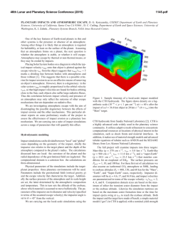
115
Ambrosi, D.: Infiltration through Deformable Porous Media
ZAMM Z. Angew. Math. Mech. 82 (2002) 2, 115––124
Ambrosi, D.
Infiltration through Deformable Porous Media
The equations driving the flow of an incompressible fluid through a porous deformable medium are derived in the framework of the mixture theory. This mechanical system is described as a binary saturated mixture of incompressible components. The mathematical problem is characterized by the presence of two moving boundaries, the material boundaries of
the solid and the fluid, respectively. The boundary and interface conditions to be supplied to ensure the well-posedness of
the initial boundary value problem are inspired by typical processes in the manufacturing of composite materials. They
are discussed in their connections with the nature of the partial stress tensors. Then the equations are conveniently
recast in a material frame of reference fixed on the solid skeleton. By a proper choice of the characteristic magnitudes of
the problem at hand, the equations are rewritten in non-dimensional form and the conditions which enable neglecting the
inertial terms are discussed. The second part of the paper is devoted to the study of one-dimensional infiltration by the
inertia-neglected model. It is shown that when the flow is driven through an elastic matrix by a constant rate liquid inflow
at the border some exact results can be obtained.
Key words: infiltration, mixture theory, inertia, Darcy’s law, porous deformable media, moving boundaries
MSC (2000): 76S05
0. Introduction
The mathematical modelling of the infiltration of an incompressible fluid through a porous deformable solid is of interest in a number of industrial and environmental applications. Notable examples are the manufacturing of composite
materials by injection molding and soil consolidation problems.
The description of the physical problem at hand can be summarized as follows. An initially dry porous medium
B with boundary @B is infiltrated by an incompressible fluid flowing through the portion of its boundary @Bin . There is
a part of the boundary (@Bwall ) which is impermeable to the fluid and another part of the boundary through which the
fluid can freely flow out (@Bout ). Both at @Bwall and at @Bout the solid matrix cannot be displaced. The body B then
consists of an infiltrated and an uninfiltrated region, Bwet and Bdry , respectively, separated by the interface S. We
assume saturation in the infiltrated region so that at each of its points only solid or fluid are possibly co-present. Then
S is a sharp interface and no air is trapped in the wet region. The process is then characterized by the occurrence of
two moving boundaries: the material boundary of the solid @B and the material boundary of the infiltrating fluid S.
The boundary of the solid defines the mathematical domain of the problem; the interface separates the infiltrated from
the uninfiltrated region (see Fig. 1).
Fig. 1 Graphical representation of the infiltration problem
A mathematical description of the infiltration dynamics has been recently addressed by several papers in the
framework of the mixture theory [1––4]. As they essentially focus on a one-dimensional description, the first aim of the
present paper is to provide a general three-dimensional statement of the problem at hand inside the mixture theory.
The equations are stated using both fixed and material coordinates, an approach close to the one of Wilmanski [5].
Real applied modelling quite often leads to initial-boundary value equations, so that the introduction of suitable
boundary conditions cannot be disregarded. This issue is here essentially connected with the understanding of the
nature of the stress acting on each component of a saturated mixture of incompressible components, the partial stress.
This long-standing subject, originally due to the pioneering work of von Terzaghi, has been recently addressed in
several papers [6, 7]. It has been shown that a precise definition of the notion of incompressibility of the constituents
by the support of microscale arguments sheds light on the nature of the partial stresses. In fact, in this approach the
tensor gradient of deformation of each component of the mixture is split into two multiplicative contributions: one
# WILEY-VCH Verlag Berlin GmbH, 13086 Berlin, 2002
0044-2267/02/0202-0115 $ 17.50þ.50/0
116
ZAMM Z. Angew. Math. Mech. 82 (2002) 2
accounting for the motion on the macroscale, the other accounting for the microscale motion [8]. For incompressible
constituents, this leads to an incompressibility constraint for each component of the mixture. Without entering into
the details of such a generalization, in this paper we discuss the controversial item of boundary conditions for a mixture and we outline under which assumptions the standard model that we adopt (essentially due to Bowen [9]) can be
understood as a special case of the general porous media theory.
In the second part of the paper the dynamics of one-dimensional infiltration when the inertial terms play a small
or negligible role is investigated. As a first step, the mechanical behavior of the solid matrix is presumed to be elastic
(see [3] for a discussion about the constitutive equations that are typically assumed concerning the specific industrial
problem of injection molding processes).
A simplifying assumption usually adopted in the literature is to neglect the inertia of the mixture in the momentum equation. This reduction in the complexity of the equations can be motivated by a dimensional analysis, that
enables showing that when the fluid pressure and solid tension balance each other the inertial terms in the momentum
equation have a minor relevance.
In order to identify when the assumption of small or negligible inertia applies, it is to be remembered that a
typical infiltration process exhibits very different dynamics when considering pressure driven or velocity driven flow. In
the former case a constant pressure drop is applied at the sponge boundaries, while in the latter case the velocity of
the inflowing fluid uin is prescribed. Pressure driven flow gives rise, for arbitrary initial conditions, to discontinuity
waves that travel back and forth in the sponge, until the equilibrium volume fraction (for a given position of the
infiltration front) is reached (see the numerical simulations reported in [2] and [3]). Then arbitrary initial conditions
yield large inertial effects with waves of permanent form, until a certain dissipation time has elapsed. On the other
hand, when the fluid infiltrates at a constant velocity uin (velocity-driven flow), no discontinuity waves are caused and
the assumptions of interest in the present paper apply.
When focusing on velocity-driven flow some exact results can be obtained for the inertia-neglected model written
in material coordinates. In fact, the equations describing the dynamics of the dry region can be integrated, simplifying
the problem from a free boundary one to a moving boundary one: the interface traveling through the mixture becomes
a boundary of the new restricted domain. The time necessary to perform a full infiltration is obtained in terms of the
length of the sponge, of the velocity of the infiltrating liquid, and of the initial state of the sponge.
The present paper is organized as follows. The first section deals with the general formulation of the mechanics
of a fluid-saturated incompressible porous medium which is partially infiltrated. Some comments concern simplified
models present in the literature that neglect the inertial terms. The equations are rewritten in a frame of reference
moving with the solid. This makes it possible to remove one of the moving boundaries of the problem, the one stating
the domain of definition of the equations. In the third section the focus is on the one-dimensional infiltration process in
a dry medium. Emphasis is given to a dimensional analysis that enables one to characterize the relative weight of the
terms in the equations and then to identify a small parameter multiplying the inertial term when the system is near
equilibrium. In Section Four the classical inertia-neglected formulation is illustrated and the equations for velocitydriven flow are partly integrated.
1. General formulation
The mathematical statement of the infiltration process within the framework of the mixture theory starts from the
introduction of the effective media concept. An observer interested in a macroscopic description of the motion of a
mixture can avoid addressing a detailed description of the microscopic dynamics, while the macroscopic one can be
properly described by the classical tools of continuum mechanics. It is to be remarked that a deterministic description
of the small-scale field is not only unuseful, but also impossible in principle, because detailed geometric data on a
porous sample cannot be obtained without destroying it. Conversely, we believe that an analysis of the equations
driving the small-scale dynamics is an essential feature for stating the macroscopic problem correctly.
Thanks to the notion of volume fraction, one formulates balance equations for both the components of the mixture, each one holding in the whole body of the mixture (see, for instance, [10––12]). In the present paper we will not
make any distinction between volume fraction and surface fraction concepts. The density of the solid and fluid component in the mixture are qs fs and ql fl , respectively, where fs ðx; tÞ is the solid volume fraction, fl ðx; tÞ is the liquid
volume fraction. The quantities qs ; ql are the real densities (also called true mass densities), which are assumed to be
constant in the present context.
Moreover, we assume that the binary mixture of incompressible constituents is saturated, that is
fs þ fl ¼ 1 :
ð1:1Þ
For the sake of simplicity, in the following we denote f :¼ fs ; fl ¼ 1 f.
By analogy with single continuum mechanics, the equations driving the dynamics of the components of the
mixture are postulated to be
@f
þ divðfvs Þ ¼ 0 ;
ð1:2Þ
@t
Ambrosi, D.: Infiltration through Deformable Porous Media
@f
þ divðð1 fÞ vl Þ ¼ 0 ;
@t
@
~s ¼ m ;
ðfvs Þ þ qs divðfvs vs Þ div T
qs
@t
@
~ l ¼ m ;
ðð1 fÞ vl Þ þ ql div ðð1 fÞ vl vl Þ div T
ql
@t
117
ð1:3Þ
ð1:4Þ
ð1:5Þ
where vs ðx; tÞ is the velocity of the solid component, vl ðx; tÞ is the velocity of the liquid component, m is the (internal) force acting between the components and I is the identity tensor. Eqs. (1.2)––(1.3) express the conservation of
mass for the components of the mixture, eqs. (1.4)––(1.5) express the balance of momentum for each component of the
~ l are defined when fluid and solid are co-present and should depend on the
~ s and T
mixture. The partial stress tensors T
other unknowns of the problems on the basis of a proper constitutive relationship. However, note that, because of their
own definition, it is intrinsically impossible to determine them experimentally. For instance, no measurement can be
performed on the solid matrix alone when the fluid is co-present.
Summing up eqs. (1.2) and (1.3) we get the kinematic saturation constraint that the mixture has to satisfy in its
motion:
divðfvs þ ð1 fÞ vl Þ ¼ 0 :
ð1:6Þ
It is possible to sum the momentum eqs. (1.4) and (1.5), thus obtaining a momentum equation for the mixture,
where the interaction force does not appear. Such an equation can be conveniently considered instead of (1.4). Define
the density and momentum of the mixture as follows:
q :¼ qs f þ ql ð1 fÞ ;
ð1:7Þ
qv :¼ qs fvs þ ql ð1 fÞ vl :
ð1:8Þ
Then summing up the momentum equations for the single components yields
@
~ ¼ 0;
ðqvÞ þ divðqv vÞ div T
@t
ð1:9Þ
where
~ :¼ T
~s þ T
~ l qs fðv vs Þ ðv vs Þ ql ð1 fÞ ðv vl Þ ðv vl Þ :
T
ð1:10Þ
It is to be remarked that the concept of “velocity of the mixture” is a matter of definition and, even though eq. (1.8) is
assumed to provide such a quantity, the constraint (1.6) does not apply to it. Nevertheless, eq. (1.9) is the only
momentum equation that could be experimentally verified, at least in its inertia-neglected form. The equations holding
for the single constituents, although they are stated at the very beginning of the theory, are actually designed in order
to provide a theoretical background for (1.9).
The partial stress of the components is now decomposed into a pressure part and an excess stress, which is
supposed to be zero for the fluid component:
~ s ¼ Ts fpI ;
T
~ l ¼ ð1 fÞ pI ;
T
~ ¼ T pI :
T
ð1:11Þ
The absence of excess stress for the fluid component assumes implicitly that any viscous effect is accounted for by the
internal force m. The pressure p should be correctly interpreted as the Lagrange multiplier that ensures the accomplishment of the constraint (1.6). At this stage there is no apparent reason to identify it as the pressure of the liquid in
the pores.
The introduction of the Lagrange multiplier p into the momentum equations can be carried out by standard
arguments from thermodynamics, exploiting the entropy principle. Writing down the saturation constraint in terms of
velocities enables one to obtain that each partial stress contributes at the mixture pressure p proportionally to its void
ratio, as appears in (1.11) (see for instance [9]). It is to be mentioned here that the introduction of a unique saturation
constraint (and then a unique Lagrange multiplier) is not the most general approach that one can conceive. de Boer
and coworkers have recently shown [6–8] that the deformation gradient of each component can be multiplicatively
decomposed into a macroscopic tensor, which describes the deformation at the microscale, and a tensor which reflects
the remaining part of the control space. Then the incompressibility of each constituent reads as a a constraint that
calls for a Lagrange multiplier. It follows that for a saturated binary mixture of incompressible constituents three
Lagrange multipliers are to be supplemented in principle, of which only two are independent. Without detailing the
theory and referring to the quoted papers, we just mention that the introduction of the unique pressure p reads as a
particular case of the more general porous media theory. It involves the tacit assumption that the three Lagrange
multipliers of the general theory are equal. In this respect, we do not discuss the thermodynamical admissibility of the
formulated model, as it can be viewed as a particular case of the general theory, whose thermodynamical foundations
can be found in the cited literature.
118
ZAMM Z. Angew. Math. Mech. 82 (2002) 2
Different assumptions are often made in order to simplify the momentum eq. (1.9), leading to different sets of
equations to be solved. We list here some of the approaches encountered in the literature.
1. All the inertial terms are assumed to be negligible. In such a case the momentum eq. (1.9) reduces to a balance
between the solid stress and pressure:
divðT pIÞ ¼ 0 :
ð1:12Þ
2. The nonlinear convective terms are omitted in eqs. (1.4) and (1.5), thus assuming that the velocities and deformations are so small that their contribution in the quadratic terms is negligible, though their derivatives are not.
When considering the fully linearized equations, with a linear elastic stress tensor Ts , the Biot equations for a
mixture of incompressible constituents are (rigorously) recovered and an analysis of this problem in terms of plane
waves is possible [13].
3. Only the inertial terms corresponding to the fluid mass are negligible. This simplification is possible when the fluid
density is much smaller than the solid one and (1.9) simplifies to
@
ðfvs Þ þ divðqs fvs vs Þ divðT pIÞ ¼ 0 :
ð1:13Þ
qs
@t
In the first part of the present paper we focus on the model that follows from the assumptions outlined under
the third point. Consequently, we neglect the inertial terms in the momentum equation for the fluid component (1.5),
too; furthermore, we postulate a dependence of the internal force m on the other unknowns as follows:
m ¼ ð1 fÞ2 mK1 ðvl vs Þ þ p grad f ;
ð1:14Þ
where K is the permeability tensor and m the dynamic viscosity of the fluid (see for instance [10], page 23, [14]). Then
we get a very simplified momentum equation for the fluid component, Darcy’s law [10]:
K
ð1:15Þ
ð1 fÞ ðvl vs Þ ¼ grad p :
m
For Darcy’s law the pressure gradient is a bulk force proportional to the mutual velocity of solid and fluid. It can be
shown by arguments of energetic type that it has a dissipative nature.
1.1 Boundary conditions
In the following we focus on the problem defined by (1.2), (1.6), and (1.13), where the pressure is eliminated from the
problem thanks to (1.15). The equations at hand are therefore, in Bwet , that
@f
þ divðfvs Þ ¼ 0 ;
ð1:16Þ
@t
ð1:17Þ
divðfvs þ ð1 fÞ vl Þ ¼ 0 ;
@
ðq fvs Þ þ divðqs fvs vs Þ r T ¼ mð1 fÞ K1 ðvl vs Þ :
ð1:18Þ
@t s
In the uninfiltrated portion of the sponge we assume that the air flow does not contribute to the dynamics of the
infiltration and then, in Bdry ,
@f
þ divðfvs Þ ¼ 0 ;
ð1:19Þ
@t
@
ðfvs Þ þ divðqs fvs vs Þ r Ts ¼ 0 :
ð1:20Þ
qs
@t
At the boundary of the mixture such systems of equations call for boundary conditions providing the value of the
velocity field (respectively, the displacement) of the mixture or the value of the forces acting at the boundary. However, the boundary conditions to be prescribed for a mixture are still a matter of debate. The difficulty of the problem
lies in the inherent difficulty in supplying continuity of quantities (say, the stress) that have different nature in the
mixture and out of it. In fact, the mixture is postulated to satisfy equations that have been derived from the equations
valid at the microscopic level (and in the outer environment) by an averaging procedure. What relationship do exist
between the stress obtained by such an averaging and the “standard” stress of the components that face the boundary
of the mixture?
Despite the fact that the matter is controversial, some results are available for specific problems. For instance,
assuming no entropy flux and no temperature jump Liu [15] has shown that the chemical potential of the component
flowing through a semi-permeable surface is continuous. In the specific case of a porous medium saturated by an elastic
fluid, this results in the continuity of the external pressure of fluid P and pressure p in the mixture. Liu claims that
correct boundary conditions for the mixture can be provided only by enforcing continuity of fluxes of the whole mixture, not of the single components. He is probably driven to this conclusion by the inconsistency that would originate
from assuming the continuity of the stress as provided by eq. (1.5), where the pressure times the liquid volume fraction
appears.
119
Ambrosi, D.: Infiltration through Deformable Porous Media
Following Mannseth [16], in this paper we assume that jump rules derived from single-component equations
hold, but they are to be considered in their fully specified form, i.e., when also possible interaction terms are explicitly
detailed. In the specific case of the fluid flow, the momentum equation with explicit inclusion of the interaction term
(1.15) has to be considered, thus leading to continuity of fluid pressure and mixture pressure tout court. Without discussing this item any further (the interested reader may refer to the relevant literature [15––18]) the assumptions above
lead to the following set of boundary conditions that characterize the manufacturing processes of composite materials:
P ¼ p;
0 ¼ T n
vl n ¼ uin
at @Bin ;
ð1:21Þ
½½fðvs vl Þ n ¼ 0 ;
½½qs fvs ðvs vl Þ T n ¼ 0
across S ;
ð1:22Þ
vs ¼ 0
at @Bout ;
ð1:23Þ
vl n ¼ vs n ¼ 0
at @Bwall :
ð1:24Þ
Here nðx; tÞ is the outgoing unit vector normal to the surface under consideration, uin is the prescribed velocity of the
fluid (which is not the inflow rate) and ½½a denotes the jump of a across the interface. Note that the normal component of the fluid velocity at the interface S is by definition the velocity of the interface itself, as it is a material
boundary of the fluid.
2. Lagrangean framework
The problem defined by (1.3), (1.6), (1.13), and (1.15) can be conveniently restated in a frame of reference fixed on the
solid skeleton so that the equations hold in a domain with fixed boundary. This approach has been proposed by
Wilmanski [5] and our description resembles his formulation. However, we adopt different dependent variables that,
in our opinion, have a more immediate physical meaning and lead to a simpler form of the equations.
The equations are rewritten changing the independent variables from ðx; tÞ to ðx; tÞ, where xðx; tÞ is the position
that the particle located in x at time t has in the reference (relaxed) configuration. We denote by B0 the position of the
body in the reference configuration. By standard arguments (see [19]) the equations in a Lagrangean frame of reference
read, in B0wet
@
ðJð1 fÞÞ þ r ðð1 fÞ ðvl vs Þ JFT Þ ¼ 0 ;
@t
ð2:1Þ
r ððfvs þ ð1 fÞ vl Þ JFT Þ ¼ 0 ;
ð2:2Þ
@
ðfvs JÞ r ððT pIÞ JFT Þ ¼ 0 ;
ð2:3Þ
@t
K
ð2:4Þ
ð1 fÞ ðvl vs Þ J ¼ r ðpJFT Þ ;
m
where r represents the divergence differential operator in the moving reference frame, F is the tensor gradient of
deformation of the solid skeleton, J ¼ fr =f is its determinant, fr is the solid volume fraction in the reference state and
the superscript T indicates the transpose of the inverse matrix. In terms of the void ratio e :¼ ð1 fÞ=f, the equations read
@e
þ r ðeðvl vs Þ FT Þ ¼ 0 ;
ð2:5Þ
@t
qs
r ððvs þ evl Þ FT Þ ¼ 0 ;
@
vs r ððT pIÞ ðe þ 1Þ FT Þ ¼ 0 ;
qs
@t
K
eðvl vs Þ ¼ r ðpðe þ 1Þ FT Þ :
m
Again, it is possible to eliminate the pressure from the problem using (2.8); thus (2.7) reads
@
vs r ðTðe þ 1Þ FT Þ ¼ meK1 ðvl vs Þ ;
qs
@t
which has to be considered with (2.5) and (2.6). In B0dry the following equations hold:
@e
þ r ðeðvl vs Þ FT Þ ¼ 0;
@t
r ððvs þ evl Þ FT Þ ¼ 0 ;
@
vs r Ts ðe þ 1Þ FT ¼ 0 :
qs
@t
Here vl denotes the velocity of the air, which is assumed not to play any dynamic role.
ð2:6Þ
ð2:7Þ
ð2:8Þ
ð2:9Þ
ð2:10Þ
ð2:11Þ
ð2:12Þ
120
ZAMM Z. Angew. Math. Mech. 82 (2002) 2
2.1 Moving surface and boundary conditions
In the section above the equations have been rewritten in terms of coordinates fixed on the solid skeleton, so that the
boundary of the overall domain of definition of the problem is fixed. Now the velocity of the infiltration front, which
moves for a fixed observer with velocity vl , has to be rewritten in the new coordinate frame.
Consider the surface inside the mixture moving with velocity vl , which is different from the material velocity of
the mixture. We want to state at which speed the surface is seen to move by the observer in the coordinate system
fixed on the solid. This velocity results in the difference between the velocity of the surface and the one of the reference
frame; moreover this vector has to be transformed from the physical (moving) domain to the (fixed) reference one by
the operator F1 [5, 20]:
n ¼ F1 ðvl vs Þ :
ð2:13Þ
Boundary conditions for the equations written in material reference frame read
P ¼ p;
^ ¼ uin
vl FT n
^;
0 ¼ TFT n
½½Jqs vs n JTðe þ 1Þ F
T
^ ¼ 0;
n
at @B0in ;
ð2:14Þ
0
across S ;
ð2:15Þ
@B0out
vs ¼ 0
at
;
ð2:16Þ
^ ¼ vs FT n
^¼0
vl FT n
at @B0wall :
ð2:17Þ
^ is the outgoing unit vector normal to the surface under consideration in its relaxed configuration. The analogue
Here n
of the first condition of (1.22) does not appear in the list above, as it now simply states that the velocity of the interface in Lagrangean coordinates n is well defined by (2.13), because the right hand side of such an equation is a quantity continuous across the interface itself.
3. One-dimensional infiltration
In this section we focus on the infiltration process through a porous deformable one-dimensional medium (in the following also referred to as sponge), with physical boundaries located at x ¼ x0 ðtÞ and x ¼ x2 ¼ L. We assume from now on
that both the mixture and the dry solid exhibit the same elastic behavior given by the stress function T ¼ T ðfÞ where
dT =df < 0; 8f.
At t ¼ 0 the sponge is completely dry and the fluid starts flowing in from x0 ¼ 0, at the velocity uin . The material boundary of the liquid is at x1 ðtÞ, so that the infiltrated region is ½x0 ðtÞ; x1 ðtÞ.
In material coordinates, the evolution of the fluid-sponge mechanical system in the wet region is described by the
one-dimensional counterpart of eqs. (2.5), (2.6), and (2.9):
@e
@
e
þ ðer þ 1Þ
ðvl vs Þ ¼ 0 ;
ð3:1Þ
@t
@x e þ 1
@ vs þ evl
¼ 0;
ð3:2Þ
@x
eþ1
qs
@vs
@T me
¼
ðer þ 1Þ
ðvl vs Þ ;
@x K
@t
ð3:3Þ
where x 2 ½0; x1 ðtÞ, er :¼ ð1 fr Þ=fr is the void ratio in the reference configuration and, in general, K ¼ KðeÞ.
As a remarkable simplification, in one spatial dimension the kinetic constraint (3.2) immediately provides a first
integral of the motion, the composite velocity
vs þ evl
¼ uin ðtÞ :
eþ1
ð3:4Þ
We can then represent the fluid velocity in terms of the other unknowns, so that the system of equations driving the
flow in the wet region ½0; x1 ðtÞ is finally
@e
@
þ ðer þ 1Þ
ðuin vÞ ¼ 0 ;
@t
@x
qs
@v
@e
m
T0
¼
ðe þ 1Þ ðuin vÞ ;
@t
@x K
ð3:5Þ
ð3:6Þ
where T 0 :¼ dT =de. For simplicity of notation from now on we denote the solid velocity vs :¼ v, as it is the only
velocity to be considered in the following.
121
Ambrosi, D.: Infiltration through Deformable Porous Media
In the dry region equations are analogous to (3.5) and (3.6), but now the friction between fluid (the air) and
solid is supposed to be negligible for the overall dynamics so that the system of equations simplifies to
@e
@
þ ðer þ 1Þ
ðuin vÞ ¼ 0 ;
@t
@x
qs
ð3:7Þ
@v
@e
T0
¼ 0;
@t
@x
ð3:8Þ
which has to be solved in ½x1 ðtÞ; L.
The boundary conditions (2.14), (2.15), and (2.16) simplify as follows:
0 ¼ T ðeÞ
vl ¼ uin
at x ¼ 0 ;
ð3:9Þ
½½qs vx_1 T ¼ 0
across x1 ðtÞ ;
ð3:10Þ
vs ¼ 0
at x ¼ L :
ð3:11Þ
Note that the condition corresponding to the second of (2.14) does not appear in the list above because it has already
been used when integrating the incompressibility constraint in (3.4). When specializing (2.13) to the one-dimensional
case we get
f
er þ 1
ðuin vÞ :
ð3:12Þ
x_1 ¼ ðvl vÞ ¼
fr
e
x1
x1
3.1 Non-dimensional equations
The governing eqs. (3.5)––(3.12) are now conveniently rewritten in non-dimensional form. The choice of the reference
magnitudes for the quantities to be rescaled is crucial: as we are interested in studying the behavior of the mechanical
system near equilibrium, that is when stress and internal forces balance, we choose as typical scales the ones that
characterize the equilibrium state. Therefore, letting uin be the reference value for scaling the velocities and L the
reference length, the equations can be recast in non-dimensional form:
@e
@
þ ðer þ 1Þ
ð1 v^Þ ¼ 0 ;
@t
@x
E
ð3:13Þ
@^
v ^0 @e
eþ1
T
¼ ð1 v^Þ
;
^
@t
@x
K
ð3:14Þ
where
v^ :¼
v
;
uin
T ðeÞ
;
T^ðeÞ :¼
T ðeeq Þ
tuin
t^ :¼
;
L
^ ðeÞ :¼ KðeÞ ;
K
Kðeeq Þ
x
x^ :¼ :
L
Eqs. (3.13) and (3.14) hold for 0 < x^ < x^1 where the equilibrium void ratio eeq is the solution of the following nonlinear
algebraic equation:
T 0 ðeeq Þ
muin
¼
;
L
Kðeeq Þ
ð3:15Þ
and the parameter E is defined by
E :¼
qs uin Kðeeq Þ
:
mL
ð3:16Þ
For simplicity of notation, we drop the sign “^” as only non-dimensional quantities will be considered in the following.
Typically near equilibrium E 1 and, following the terminology of [21, 22], eqs. (3.13)––(3.14) form a nonlinear
hyperbolic system with stiff diffusive relaxation defined for a moving domain.
In the dry region, the following equations hold:
@e
@
ð1 vÞ ¼ 0 ;
þ ðer þ 1Þ
@t
@x
E
@v
@e
T0
¼ 0;
@t
@x
ð3:17Þ
ð3:18Þ
for x1 < x < 1. The boundary conditions (3.9), (3.10), and (3.11) in dimensionless form read
0 ¼ T ðeÞ
at x ¼ 0 ;
ð3:19Þ
½½Evx_1 T ¼ 0 ;
across x1 ðtÞ ;
ð3:20Þ
v¼0
at x ¼ L ;
ð3:21Þ
122
and
ZAMM Z. Angew. Math. Mech. 82 (2002) 2
er þ 1
ð1 vÞ :
x_1 ¼
e
x
1
ð3:22Þ
4. The inertia-neglected model
When neglecting the inertial terms completely (E ¼ 0), the system (3.13)––(3.14) reduces to a scalar parabolic equation.
Define first
KT 0
> 0:
ð4:1Þ
fðeÞ ¼ ðer þ 1Þ
eþ1
For vanishing inertial terms, eq. (3.14) is not evolutive any more and straightforwardly provides the flux of (3.13),
v¼1þ
1
@e
1
@e
fðeÞ
KT 0
¼1þ
;
eþ1
@x
er þ 1
@x
ð4:2Þ
@e @
@t @x
@e
fðeÞ
¼ 0;
@x
ð4:3Þ
yielding
which is the parabolic equation describing the flowfield in the wet region. Using (4.2) eq. (3.22) now reads
_x ¼ 1 fðeÞ @e :
1
e
@xx1
ð4:4Þ
Let us consider the dry region. As the fluid pressure is absent, for E ¼ 0 eq. (3.18) trivially says that the void
ratio does not depend on x. In such a context some exact results can be obtained.
Billi and Farina [4] have studied the pressure-driven problem (4.3) for applied constant pressure drop DP . In
this case the void ratio in the dry region instantaneously reaches the value e ¼ ec , where ec ¼ T 1 ðDP Þ. Then eq.
(4.3) with boundary movement (4.4) is a Stefan-like problem, which can be shown to have a unique self-similar solution, with interface position growing in time as t1=2 .
Also if the fluid flows in through x ¼ 0 at a constant rate 1 (velocity-driven flow), the value of the void ratio is
constant throughout the dry region, but changes in time. Now eq. (3.17) simplifies to
de1
@v
;
¼ ðer þ 1Þ
@x
dt
ð4:5Þ
where e1 ðtÞ :¼ eðx ¼ 1; tÞ. Eq. (4.5) can be immediately integrated using the boundary condition (3.21):
ðer þ 1Þ vðx; tÞ ¼
de1
ðx 1Þ ;
dt
x1 < x < 1 :
ð4:6Þ
Now the solution of the equations holding in the wet region (4.3) and in the dry region (4.5) have to be matched at
the interface by enforcing the continuity requirement (3.20). For neglected inertia, this relationship just expresses the
continuity of the stress across the interface. Because of our assumption of identical mechanical behavior of elastic type
of the dry and wet sponge, the stress SðfÞ being a strictly monotone function, this requirement is equivalent to imposing continuity of the void ratio e. Then, for conservation of mass, the velocity also has to be continuous across the
interface. Equating (4.2) and (4.6) evaluated in x ¼ x1 yields
@e de1
:
ð4:7Þ
er þ 1 þ fðeÞ ¼ ðx1 1Þ
@x x1
dt
Using (4.4) eq. (4.7) can be rewritten as
d
ðe1 ð1 x1 ÞÞ ¼ er þ 1 ;
dt
ð4:8Þ
which can be integrated from the initial conditions corresponding to the relaxed state
e1 ð1 x1 Þ ¼ er ðer þ 1Þ t :
As a by-product, it immediately follows that the sponge is completely infiltrated at t ¼ tfin , such that
er
:
tfin ¼
er þ 1
ð4:9Þ
ð4:10Þ
Note that also in dimensional variables the infiltration time is independent of the mechanical characteristics of the
sponge.
Ambrosi, D.: Infiltration through Deformable Porous Media
123
Thanks to the integration above, the infiltration problem can now be restated in the wet domain only: eq. (4.3)
has to be solved in ½0; x1 ðtÞ, where the movement of the right border obeys (4.4) and the boundary conditions are
supplemented by (3.19) and (4.9):
ð4:11Þ
eð0Þ ¼ er ;
eðx1 Þ ¼
er ðer þ 1Þ t
:
1 x1
ð4:12Þ
A simple mass-balance calculation allows one to see that the material fluid boundary, that moves with the
velocity given by (4.4), specifies a very special case of boundary motion, such that there is no flow of void ratio e
across the interface. In fact, consider the integral of (4.3) in the wet region,
xð1
@e
dx @t
0
xð1
@
@x
f
@e
dx ¼ 0 :
@x
ð4:13Þ
0
We can extract the time derivative from the integral symbol, thus getting
d
dt
xð1
@e @e e dx x_1 e f
þf
¼ 0;
x1
@x x1
@x 0
ð4:14Þ
0
and, because of (4.4), the contribution of the interface vanishes:
d
dt
xð1
e dx ¼ f
@e :
@x 0
ð4:15Þ
0
5. Final remarks
A formulation of the infiltration process through a deformable porous medium has been stated in the framework of the
mixture theory, with quite general assumptions concerning the constitutive relationships to be supplemented. Such a
description essentially resembles the one by Wilmanski, but with a different choice of dependent variables and some
more emphasis on boundary conditions. Focusing on one-directional processes it has been shown that when the solid
exhibits a linear elastic behavior and the inertia can be neglected, the equations can be partly integrated and the final
problem reads as a nonlinear parabolic equation with non-standard boundary conditions.
Several items are still to be investigated for the problems at hand. In the author’s opinion, major ones are the
absence of a general theory for admissible boundary conditions to be supplied at the boundary of a mixture and the
necessity to specify the above theory in terms of more realistic constitutive relationships. As discussed in Section 1, the
model adopted in this paper can be approached as a particular case of the more general porous media theory. It is still
to be investigated to what extent the results above retain their validity in the general framework. Finally, it is to be
remarked that the reduction to the inertia-neglected model carried out in Section 4 does not ensure at all that for
E ! 0 the solution of the complete system of equations tends to the E ¼ 0 one. This issue requires that a singular
perturbation analysis be carried out in the near future.
Acknowledgements
The author is indebted with Luigi Preziosi, Renato Lancellotta, and Andrea Cortis for several fruitful discussions about the
content of this paper. The reviewers of the journal are deeply acknowledged for their comments. This research has been supported by
Italian GNFM.
References
1 Preziosi, L.: The theory of deformable porous media and its application to composite material manufacturing. Surveys Math. for
Industry 6 (1996), 167––214.
2 Ambrosi, D.; Preziosi, L.: Modelling matrix injection through porous preforms. Composites A 29 (1998), 5––18.
3 Ambrosi, D.; Preziosi, L.: Modelling injection moulding processes with deformable porous preforms. SIAM J. Appl. Math. 61
(2000), 22––42.
4 Billi, L.; Farina, A.: Unidirectional infiltration in deformable porous media: mathematical modelling and self-similar solution.
Quart. Appl. Math. 58 (2000), 85––101.
5 Wilmanski, K.: Lagrangean model of two-phase porous material. J. Non-Equil. Thermodyn. 20 (1995), 50––77.
6 Bluhm, J.; de Boer, R.; Wilmanski, K.: The thermodynamic structure of the two-component model of porous incompressible
materials with true mass densities. Mech. Res. Commun. 22 (1995) 2, 171––180.
124
ZAMM Z. Angew. Math. Mech. 82 (2002) 2
7 de Boer, R.: Saturated compressible and incompressible elastic porous solids. ZAMM 77 (1997), S397––S400.
8 de Boer, R.: The thermodynamic structure and constitutive equations for fluid-saturated compressible and incompressible porous
solids. Int. J. Solids Struct. 35 (1998), 4557––4573.
9 Bowen, R. M.: Incompressible porous media models by use of the theory of mixtures. Int. J. Eng. Sci. 18 (1980), 1129––1148.
10 Rajagopal, K. R.; Tao, L.: Mechanics of mixtures. World Scientific, Singapore 1995.
11 de Boer, R.: Theory of porous media: past and present. ZAMM 78 (1998), 441––466.
12 Bowen, R. M.: Theory of mixtures. In: Eringen, A. C. (ed.): Continuum physics. Academic Press, 1976.
13 Liu, Z.; Bluhm, J.; de Boer, R.: Inhomogeneous plane waves, mechanical energy flux and energy dissipation in a two-phase
porous medium. ZAMM 78 (1998), 617––625.
€ hnk, K.; Svendsen, B.: On interfacial transition conditions in two phase gravity flow. Z. angew. Math. Phys.
14 Hutter, K.; Jo
45 (1994), 746––762.
15 Liu, I. S.: On chemical potential and incompressible porous media. J. MNec. 19 (1980) 2, 327––342.
16 Mannseth, T.: On the fluid-phase momentum balance laws and momentum jump condition for porous media flow. Eur. J.
Mech./B Fluids 10 (1991), 97––111.
17 Beavers, G. S.; Joseph, D. D.: Boundary conditions at a naturally permeable wall. J. Fluid Mech. 30 (1967), 197––207.
18 Payne, L. E.; Straughan, B.: Analysis of the boundary conditions at the interface between a viscous fluid and a porous medium and related modelling questions. J. Math. Pur. Appl. Anal. 77 (1998), 317––354.
19 Gurtin, M. E.: An introduction to continuum mechanics. Academic Press, New York 1981.
20 Gurtin, M. E.: The nature of configurational forces. Arch. Rat. Mech. Anal. 131 (1995), 101––119.
21 Liu, T. P.: Hyperbolic conservation laws with relaxation. Comm. Math. Phys. 108 (1987), 153––175.
22 Chen, G. Q.; Levermore, C. D.; Liu, T. P.: Hyperbolic conservation laws with stiff relaxation terms and entropy. Comm. Pure
Appl. Math. 47 (1994), 787––830.
Received June 13, 2000, revised December 19, 2000, accepted December 20, 2000
Address: Prof. Davide Ambrosi, Dipartimento di Matematica, Politecnico di Torino, corso Duca degli Abruzzi 24, I-10129 Torino,
Italy, e-mail: [email protected]