1. Art and Diseño

Relative Convergence and
Cross-Section Dynamics:
A New Approach to Convergence
Gerard H. Kuper
SOM theme C: Coordination and Stabilization of Economic Systems
Abstract
This paper analyses income convergence between groups of countries
relative to world-wide development. The alternative to conventional convergence tests introduced here provides more transparent and intuitively
more reasonable results. Using a combination of cross-section data and
time series data for the period 1970{1990 we nd evidence for a separation in levels of income (measured as real per capita GDP) between
groups of countries. Africa seems to be trapped in a situation with a low
level of real per capita GDP, whereas the OECD countries nd themselves in a position with a relatively high level of real per capita GDP.
Latin America diverges and Asia converges relatively to world-wide development.
Keywords: Panel data, Income convergence, Economic growth
JEL-classication: C33, O10, O50
CCSO and Department of Economics, University of Groningen, PO Box 800, 9700 AV
Groningen, The Netherlands, Email: [email protected]. I would like to thank Jan Jacobs, Simon Kuipers and Jan Egbert Sturm for comments and suggestions.
1
1 Introduction
A vast, and still growing, literature has appeared over the last decade dealing with the question: Do countries or groups of countries have a tendency
to converge in terms of the levels of income or GDP per capita ( convergence)? And related to that: If countries do not seem to converge, do they
so after holding xed variables that capture dierences in cultures, institutions and policies (conditional convergence)? See, for instance, Barro and
Sala-i-Martin's 1995 book on Economic Growth and many other papers for
references on convergence and conditional convergence. Obviously, the SolowSwan neoclassical growth model from the 1950s predicts conditional convergence (see Romer (1986)). The stylized facts however, show large|and indeed
growing|dierences in income over time and across countries. This has led to
a diverse body of theoretical and empirical literature on|what is now known
as|endogenous growth theory. For a discussion we refer to the Policy Forum
in The Economic Journal of 1992 and to the contributions on endogenous
growth in the Journal of Economic Perspectives in 1994. In particular, we
refer to Dowrick's contribution on catch up and divergence in The Economic
Journal and to Romer (1994) and Pack (1994).
The convergence hypothesis is usually tested by a regression of average
growth rates on initial levels in a cross-country setting. The lower the starting
level of real per capita GDP (or income) relative to the steady state position,
the faster is the growth rate (due to the assumption of diminishing returns to
capital). A negative coecient in these so-called Barro-regressions indicates
that countries with a low initial level of income grow faster than countries
with higher initial levels of income. This is what is meant by convergence or
convergence. From theoretical and empirical studies it is quite clear that
convergence only happens if rms and households in countries or groups of
countries have the same tastes and technology, including education. This is
nicely illustrated in Barro and Sala-i-Martin (1995): convergence is weak, or
absent, between OECD countries on the one hand and Latin-American and
African countries on the other hand and there seems to be some convergence
within the OECD. Convergence is apparently present between more homogeneous regions (in terms of tastes and technology) within countries like the U.S.
states and the regions of Japan.
Quah (1993a) shows that these kinds of tests based on cross-country data
lead to the wrong conclusions because the estimation results are biased due
2
to regression-to-the-mean (or Galton's regression to mediocrity). Furthermore,
Quah suggests to get rid of world-wide co-movements in growth of per capita
income by normalizing per capita income for each country because convergence
is disturbed by global growth of per capita income. Barro and Sala-i-Martin are
aware of the biases due to regression-to-the-mean problems as their remarks on
page 32 and page 383 (footnote 1) in their book indicate. However, they believe
that the problem is irrelevant and perhaps most obvious for ordinal rankings.1
Ben-David (1994, 1995) avoids cross-country regressions altogether and relies
on time-series information for determining (lack of) convergence. This seems
reasonable since convergence is, by denition, a dynamic concept which cannot
be captured by cross-section studies. Combining time-series analysis in a crosscountry setting introduces the dynamics needed to analyse convergence in a
proper manner.
This paper corroborates Quah's opinion that standard regressions may easily
lead to the wrong conclusions because of regression-to-the-mean problems.
Moreover, it shows that normalization of income per capita in a dynamic
time-series analysis shows more clearly whether or not convergence occurs.
The data we use here are derived from the International Financial Statistics
of the IMF. We have gathered information on real GDP per capita for a
number of countries for the period 1970{1990. The data appendix provides
more detail. Our conclusions clearly point at a \: : : tendency towards a twocamp world divided between haves and have-nots : : : " (Quah (1993b), page
433). Quah reaches the same conclusion by analysing the income distribution
across entire economies using a Markov chain transition model. Our analysis
is much simpler and similarly transparent.
2 Stylized facts
The stylized facts point at large dierences in levels of real per capita GDP
between countries as well as large dierences in rates of growth of real per
capital GDP. The top half of gure 2.1 (the dotted lines) shows the initial
levels of per capita GDP in 1970 (GDPL70) and 1990 (GDPL90) for about 73
We think that this defense of the conventional convergence analysis is not very convincing
since, as far as we know, Galton himself did not use ordinal data. Furthermore, Quah (1993a)
clearly points out that this kind of cross-section regressions are completely uninformative for
the dynamics of the distribution.
1
3
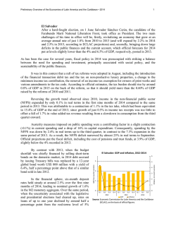
Figure 2.1
Annual growth rate of real per capita GDP, 1971{1990 and levels of per
capita GDP in 1970 (- - -) and 1990 ({ { {) for 73 countries
countries: the bottom half lists the average annual rates of growth of real per
capita GDP during the period 1971{1990 (GDPR7190).
Latin-American countries and African countries show hardly any improvement in levels of real per capita GDP, whereas the rates of growth show a large
variation. For OECD countries (including Japan) rates of growth of real per
capita GDP are on average moderate but positive and the levels of real per
capita GDP increase signicantly. Asian countries (eastern and western Asian
countries taken together) grow faster, on average, than OECD countries. If
one is to expect convergence one would expect it to be the case for Asian
countries.
Table 2.1 shows sharp dierences in growth rates over time and across regions. In the 1970s most countries experienced positive growth, whereas in the
1980s the Latin-American countries show on average a decline in per capita
GDP.
4
Table 2.1
Average annual rates of growth of real per capita GDP
Annual growth rates of real per capita GDP
period
1971{1975
1976{1980
1981{1985
1986{1990
Latin America Africa
2:44
1:79
2:15
0:08
2:46
0:31
0:01
0:93
Asia
4:56
4:41
2:40
3:79
OECD World
2:83
2:63
1:64
2:65
2:89
2:13
0:26
1:62
In the period 1971{1975 rates of growth of real per capita GDP ranged from
-3.6% for Chile to 17.6% for Pakistan. The average annual growth rate for the
period 1976{1980 ranged from -9.3% for Zaire to 7.8% for Botswana. Malta
(not in our sample of 73 countries since Malta does not belong to the OECD
and we did not include non-OECD European countries) experienced massive
growth of about 12.3% on average in the same period. The highest average rate
of growth in the periods 1981{1985 and 1986{1990 is found in Korea, whereas
the lowest rate of growth is found in Bolivia for the period 1981{1985 and in
Nicaragua for the period 1986{1990. The highest rates of growth are typically
found in Asia, and the lowest rates of growth in the African countries. The
gures displayed in table 2.1 conrm Baumol's remark that \: : : there is more
than one convergence club, : : : poorer less developed countries are still largely
banned from the homogenization process : : : " (Baumol (1986), p. 1080).
3 Conventional convergence tests
Quah's criticism on traditional convergence tests captures the notion that although levels of real per capita GDP in Latin-American countries and African
countries increase, their levels of real per capita GDP decrease relative to
world-wide growth. That is, countries which little or no growth in fact fall
back in terms of standard of living: \: : : economic growth, to the extent that it
increases socially unrealisable aspirations, may actually reduce social welfare
: : : " (Ng (1983), p. 277).
5
Before we discuss this critique in more detail, we rst estimate2 the basic
equation used for testing convergence by Barro and Sala-i-Martin (1995, p.
384). The rate of growth of real per capita GDP is regressed on a constant
and the initial level of real per capita GDP:
log(yi;t =yi;t 1 ) = 1 e log(yi;t 1 ) + ui;t
(1)
where yi;t is real per capita GDP for country or region i at time t, and ui;t
2
is a random variable which has 0 mean, variance u;t
, and is independently
distributed from log(yi;t 1 ), uj;t and lagged ui 's. In cross-country studies parameters and are constants (model 1 in table 3.1). Using time series data
on a panel of countries allows these parameters to dier between regions (models 2 and 3 in table 3.1). Tests on coecient restrictions can be used to test
whether or not parameters are constant across countries.
From parameter we can compute the steady-state value of y, parameter measures the speed of convergence (see Barro and Sala-i-Martin (1995)). If is the same for all countries and if > 0 in equation (1) convergence applies:
poor countries grow faster than rich countries. This is what the traditional
Solow-Swan neoclassical growth model predicts. Endogenous growth models,
like the AK-model, predict a value of 0 for , and hence no convergence.
In this section we arrive at counterintuititive and inconclusive results because the results are tainted by Galton's fallacy: > 0 in equation (1) does
not imply convergence.
Model 1 in table 3.1 shows the pooled results assuming the parameters are
equal across all countries. The t is rather poor and is not signicantly different from 0: so there seems to be no convergence. Shallow observation could
easily lead to the conclusion that the endogenous growth model is relevant.
The low Durbin-Watson (DW) test statistic hints at serious dynamic misspecication, probably caused by regression-to-the-mean. Model 2 assumes dierent
speeds of convergence across countries towards the same steady state. The t
improves. The Durbin-Watson test still hints at positive autocorrelation. The
Wald test on coecient restrictions for model 2 (reported in table 3.2) in general rejects the null hypothesis that the i 's are equal across countries. The
null hypothesis is
H0 : i = j ; 8i 6= j; i; j = 1; 2; 3; 4
We simply use the standard least squares estimators. Quah (1994) gives a rst analysis of
the subtleties that arise in unit-roots regression in data that have simultaneously extensive
cross-section and time-series variation.
2
6
Table 3.1
Parameter estimates for the basic equation, 1971{1990 (t-values between
parentheses). Subscript i indicates the region: 1=OECD, 2=Latin America,
3=Africa, 4=Asia
model 1
model 2
0:059
(2:661)
0:262
(2:212)
0:275
(0:653)
1:821
(2:399)
0:710
(1:926)
0:160
(1:239)
1
2
3
4
1
0:003
(1:541)
2
3
4
observations
R 2
DW
model 3
80
0:017
0:712
0:019
(1:998)
0:025
(2:149)
0:026
(2:023)
0:217
(1:732)
0:020
(0:593)
0:192
(2:171)
0:077
(1:804)
0:011
(0:813)
80
0:497
1:420
80
0:519
1:496
7
Table 3.2
model 2
1
2
3
2
3
4
0:01
0:04
0:41
0:35
0:00
0:00
2
3
4
0:08
0:44
0:19
0:79
0:03
0:16
model 3
1
2
3
Wald coecient restriction tests (p-values)
1
2
3
2
3
4
0:07
0:29
0:24
0:81
0:04
0:14
The null hypothesis of equal speeds of adjustment is rejected for probability
or p-values below a critical value of, say, 0.05. This test, in fact, rejects model
1.
The conclusion could be that all countries converge to the same steady state
(parameter signicantly diers from 0) at dierent speeds of adjustment.
Again, this conclusion is wrong since|as parameter restriction tests on model
3 illustrate|there is no common steady state for all countries considered.
As was mentioned before convergence requires parameter to be the same
across countries, and to be positive. Parameter is positive for all regions
in model 3, although not very signicantly dierent from 0. Whether or not
the intercept is the same in all regions is analysed using the Wald test on
coecient restrictions. Table 3.2 reports p-values for the F-test statistic on
coecient restrictions in model 3. The null hypothesis of convergence is
H0 : i = j ; 8i 6= j; i; j = 1; 2; 3; 4
From the Wald test we can conclude that 1 6= 2 (signicant at 10% only)
and 2 6= 4 (signicant at 5%). Or, in other words, the OECD (1 ) and Latin
America (2 ) do not converge to the same steady-state value of real per capita
GDP, and Latin America (2 ) and Asia (4 ) do not converge either. The null
8
of convergence is not rejected for the other combinations, not even for the
OECD and Africa!
The speed of convergence is indicated by the half-life.3 The half-life implied
by model 3 is 63 years for Asia, 35 years for the OECD, 9 years for Africa and
only 3.6 years for Latin America. Africa and Latin America seem to converge
very rapidly to their own relatively low steady states, it takes only 9 years for
Africa to make up half the dierence beween the actual level of real per capita
GDP and the steady state level, which according to the conclusion above could
well be the same steady state level as for the OECD! The OECD and Asia
move very slowly to their steady states. The hypothesis that the speed of
adjustment is the same for all countries in model 3 is rejected only for Latin
America (2 ) versus Asia (4 ) and for the OECD (1 ) versus Latin America
(2 ) (signicant at 10%).
Some of these conclusions are counterintuitive and certainly not very conclusive. Recall that a positive in these kind of regressions does not imply
convergence as Quah (1993a) has shown. Relative convergence, a concept to
be introduced in the next section, seems to be a more realistic and transparent
way to deal with subjects of income convergence and divergence.
4 Relative convergence
In order to abstract from world-wide growth, the data on real per capita
GDP for each region (OECD, Latin America, Africa and Asia) are divided by
the average levels of real per capita GDP for the group to which the countries
belong, viz. average world-wide level of real GDP (compare Ben-David (1995)).
We dene relative real per capita GDP for region i as y~i;t :
y~i;t = yi;t =yt
(2)
where yi;t is region i's average real per capita GDP at time t, and yt is the
world-wide average real per capita GDP.
Evidently, the major contribution to the world-wide level of real per capita
GDP originates from OECD countries. When we look at the income distribution across regions, table 4.1 shows that the average level of real per capita
GDP is about 2.6 times the world average level of income. The African average level of income is about 11% to 12% of the world average level of income.
3
The half-life t is derived from exp(
t) = 1=2
or t = log(2)= .
9
Table 4.1
Average real per capita GDP relative to the world-wide level of real GDP
Relative real per capita GDP
period
1971{1975
1976{1980
1981{1985
1986{1990
Latin America Africa
0:27
0:27
0:24
0:20
0:12
0:12
0:12
0:11
Asia
OECD
0:19
0:22
0:26
0:29
2:63
2:61
2:62
2:64
The second conclusion we can infer from this table is that the income distribution certainly does not show any sign of convergence. On the contrary, for
the period 1971{1990 the gap between the rich and the poor tends to widen.
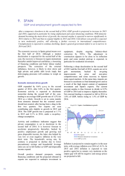
Figure 4.1 shows a scatter plot of deviations of rates of growth from the world
average rate of growth (vertical axis: YDIFGDP= log y~i;t ) and deviations
of the level of real per capita GDP from the world level of real per capita
GDP (horizontal axis: XDIFGDP=log y~i;t 1 ). Countries in the top half of the
diagram (higher than average rates of growth) and lower than average levels
of income (to the left of 0) catch up with the world steady state (relative
convergence). Those countries beat the average rate of growth. Countries in
the bottom half of the diagram and to the left of 0 move away from the
world steady state (relative divergence). Relative convergence applies for Asia,
relative divergence applies for the Latin-American countries. The OECD and
Africa more or less seem to have stabilized their relative positions with Africa
slightly falling back. For the OECD this need not come as a surprise since
most income is generated in OECD countries. Each of the four groups of
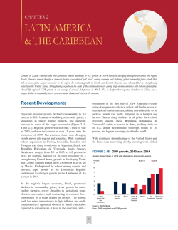
countries are plotted in more detail in gure 4.2. These plots clearly show
the dynamics. Asia, for instance, is rapidly catching up relative to the world
steady state. Latin America is falling behind, especially in the 1980s. OECD
is moving around clockwise with hardly any gain or loss. Africa is somewhat
falling behind since the early 1980s.
Some authors (see Dowrick (1995)) suggest that there is some sort of takeo threshold level of income per capita, below which economies nd it dicult
to generate the investment in education and infrastructure needed to take
advantage of the available technology. Figure 4.1 indicates that this take-o
10
Figure 4.1
Per capita growth rate versus initial per capita GDP, relative to the
group, 1971{1990
threshold level is certainly not a sucient condition for sustainable high rates
of growth. If it is, Latin America needs to be on a higher growth path, since in
the early 1970s, the initial level of income exceeded that of Asia considerably.
Edwards (1995) points at dierences in the savings rates between East Asia
and Latin America to explain why Latin America failed to take advantage of
the relatively favourable initial conditions in the 1970s.
Because the data are corrected for the world-wide development of real per
capita GDP, the development in real per capita GDP over time for one group
of countries should be interpreted in relation to world-wide growth. The rst
oilprice shock in 1974 reduced growth in the OECD and in Asia. This in turn
reduced world-wide growth and, as a consequence, growth in Africa and Latin
America peaked relative to world-wide growth. The second oilprice shock hits
Asia in 1979 and the OECD two years later. In 1983, accelerating Asian growth
reduced growth in Africa and Latin America relative to world-wide growth. In
11
Figure 4.2
Asia
OECD
Africa
Latin America
Per capita growth rate versus initial per capita GDP per region, relative
to the group, 1971{1990
12
Table 4.2
Parameter estimates for the alternative equation (t-values between
parentheses). Subscript i indicates the region: 1=OECD, 2=Latin America,
3=Africa, 4=Asia
1971{1990 1971{1980 1981{1990
1
2
3
4
observations
R 2
DW
a
0:000
( 0:087)
0:014a
( 5:592)
0:002
( 1:012)
0:022a
(9:203)
0:001
(0:198)
0:004
( 1:584)
0:001
( 0:588)
0:020a
(10:557)
0:001
( 0:212)
0:021a
( 5:737)
0:002
( 0:921)
0:025a
(5:710)
80
0:589
1:323
40
0:712
2:160
40
0:619
1:401
diers signicantly from 0 at 1%.
1985, growth in Asia dropped sharply, whereas growth in the OECD reached
record high rates of growth relative to world-wide growth.
Now, we estimate the following adjusted model, where: y~i;t is dened according to equation (2):
log(~yi;t =y~i;t 1 ) = 1 e log(~yi;t 1 ) + ui;t
(3)
Parameter is zero by construction because the data are centered around the
group average (see appendix B). This is in fact conrmed by estimation results
not reported here. Parameter measures relative convergence and is allowed to
dier between regions. A positive value for indicates relative convergence,
whereas a value of < 0 is to be interpreted as relative divergence. The
estimation results are listed in table 4.2. The rst entry gives the results for
the entire sample period. Table 4.1 above revealed rather sharp dierences in
income distribution across regions and over time, so we re-estimated the model
for the period 1971{1980 and for the period 1981{1990. These results are in
the last two columns of table 4.2.
i
13
The outcomes are in accordance with the stylized facts reported earlier:
OECD and Africa are stable relative to the world-wide development. The relative convergence parameter for the OECD countries as well as for African
countries is not signicantly dierent from 0 in both subperiods. Latin America is falling behind in the second half of the sample period, the relative convergence parameter is -0.021 in the 1980s (which is signicantly dierent from
0 at a signicance level of 1%). Asia is catching up in both subperiods: the relative convergence factor is 0.022 and diers signicantly from 0 at 1%. As far
as autocorrelation is concerned, the null hypothesis of zero autocorrelation is
not rejected for the period 1971{1980. The Durbin-Watson test is inconclusive
for the 1980s.
Compared to the results based on real per capita GDP reported in the
previous section our results are clearly more conclusive and more in line with
the facts: Latin America diverges relative to the world-wide development of
income (relative divergence of 1.4%, i.e. a double-life of 50 years), whereas Asia
converges (relative convergence of 2.2%, this implies a half-life of 32 years).
Our results conrm Romer's presumption that the relative income gap between
rich and poor tends to widen (Romer (1986)).
Furthermore, removing the bias caused by regression-to-the-mean leads to
a slightly better dynamic specication as the Durbin-Watson test statistics
suggest.
5 Conclusions
Traditional cross-country income convergence tests exhibit some shortcomings.
First, results on convergence are generally not very conclusive, especially not
in a broad selection of countries with large dierences in tastes and technology.
One way out of this problem is to select a homogeneous set of countries and
perform standard tests. However, the conclusions are then restricted to the
selected group of countries (sample selection bias).
Another problem has to do with the fact that no account is taken of an individual countries' development of income over time. Biases due to regressionto-the-mean may be the result. Correcting for the growth of income of the
group to which the countries belong in a dynamic time-series setting reduces
the estimation bias. Normalizing the data results in tests in which the convergence or divergence of countries (or group of countries) is analysed relative to
the development over time of the income of the group to which those countries
14
belong. Afterall, the theory on welfare economics shows that for the welfare
of a country its relative income (that is its income in relation to the income
of the group) may be more important than the absolute level of income of
a country. This is one of the reasons for introducing the concept of relative
convergence and relative divergence as opposed to (absolute) convergence and
divergence.
The results reported here for the period 1970{1990 show that the OECD
and Africa are relatively stable as compared to the world-wide development
of income. During the 1970s, Africa stabilized on a low level of income as
compared to the OECD. Since 1983, Africa is lagging behind. This suggests
a dichotomy in the levels of income in the world economy. Latin America is
falling behind relative to the OECD, whereas Asia is rapidly catching up.
What we nd conrms Romer's presumption that the relative income gap
between rich and poor is widening (Romer (1986)). Within regions there may
be convergence (local convergence).
The analysis in this paper is rather descriptive, relative convergence, as we
dene it here, is a proper way to summarize the stylized facts in income convergence and divergence. What we do not oer is an explanation of growth
dierences. Important questions are in this respect: Why do less developed
countries lag behind?; How can countries escape the poverty trap? Furthermore, if the developed countries are focused on growth as they are: Is it possible
for less developed countries to catch up at all?
15
References
Barro, R.J. and X. Sala-i-Martin (1995), Economic Growth, McGraw-Hill, New
York.
Baumol, W.J. (1986), \Productivity growth, convergence and welfare: What
the long-run data show", American Economic Review, 76, 1072{1085.
Ben-David, D. (1994), \Convergence clubs and diverging economies", Discussion Paper No. 922, Centre for Economic Policy Research, London.
Ben-David, D. (1995), \Trade and convergence among countries", Discussion
Paper No. 1126, Centre for Economic Policy Research, London.
Dowrick, S. (1992), \Technological catch up and diverging incomes: Patterns
of economic growth 1960{88", The Economic Journal, 102, 600{610.
Dowrick, S. (1995), \Post war growth: Convergence and divergence", Paper
for Groningen Summer School, Second Draft, 22 May, Australian National
University, Australia.
Edwards, S. (1995), \Why are savings rates so dierent across countries?",
Working Paper No. 5097, National Bureau of Economic Research, Inc.,
Cambridge, Massachusetts.
Greenaway, D. (1992), \The determinants of economic growth: Editorial note",
The Economic Journal, 102, 598{599 [Policy Forum].
International Monetary Fund, \International nancial statistics", CD-ROM,
Publications Services International Monetary Fund, Washington, D.C.
Ng, Y.-W. (1983), Welfare Economics: Introduction and Development of Basic
Concepts, revised edition, Macmillan, London.
Pack, H. (1994), \Endogenous growth theory: Intellectual appeal and empirical
shortcomings", Journal of Economic Perspectives, 8, 55{72.
Quah, D. (1993a), \Galton's fallacy and tests of the convergence hypothesis",
Scandinavian Journal of Economics, 95, 427{443.
Quah, D. (1993b), \Empirical cross-section dynamics in economic growth",
European Economic Review, 37, 426{434.
Quah, D. (1994), \Exploiting cross-section variation for unit-root inference in
dynamic data", Economics Letters, 44, 9{19.
Romer, P.M. (1986), \Increasing returns and long-run growth", Journal of
Political Economy, 94, 1002{1037.
Romer, P.M. (1994), \The origins of endogenous growth", Journal of Economic
Perspectives, 8, 3{22.
16
A Data appendix
A.1 Time-series and countries
We gathered the following time-series information from the International Financial Statistics (IFS) of the IMF for the countries listed in table A.1.
real GDP (in national currencies)
nominal exchange rate
population
The selection of countries is based on data availability. Emphasis is on timeseries so we only selected countries for which data are available for the period
1970{1990.
A.2 Conversion
Real per capita GDP is calculated as follows. First data on real GDP are
converted in US-$:
(base year 1990) in national currencies
real GDP in US-$ = real GDPexchange
rates in the base year
Second, real GDP in US-$ is divided by population:
GDP in US-$
real per capita GDP in US-$ = realpopulation
Note:
1. For some countries (Germany, Japan, Iceland and Turkey) we used real
GNP.
2. For some countries the base year is 1985.
17
Table A.1
IFS
283
288
233
213
336
299
278
228
268
223
263
218
253
369
243
343
293
273
258
238
298
248
18
List of countries
Latin America (22)
Panama
Paraguay
Colombia
Argentina
Guyana
Venezuela
Nicaragua
Chile
Honduras
Brazil
Haiti
Bolivia
El Salvador
Trinidad & Tobago
Dominican Republic
Jamaica
Peru
Mexico
Guatemala
Costa Rica
Uruguay
Ecuador
IFS
744
686
746
652
199
664
616
674
622
676
644
684
618
754
636
738
Africa (16)
Tunisia
Morocco
Uganda
Ghana
South Africa
Kenya
Botswana
Madagascar
Cameroon
Malawi
Ethiopia
Mauritius
Burundi
Zambia
Zaire
Tanzania
IFS
518
524
558
564
534
536
566
576
542
578
548
Asia (11)
Burma
Sri Lanka
Nepal
Pakistan
India
Indonesia
Philippines
Singapore
Korea
Thailand
Malaysia
IFS
112
158
156
111
146
193
144
184
142
178
138
174
137
122
136
186
134
176
132
196
172
182
128
124
OECD (24)
United Kingdom
Japan
Canada
United States
Switzerland
Australia
Sweden
Spain
Norway
Ireland
Netherlands
Greece
Luxembourg
Austria
Italy
Turkey
Germany
Iceland
France
New Zealand
Finland
Portugal
Denmark
Belgium
B Technical appendix
Dene yi;t as the average real per capita GDP for region i = 1; : : : ; K at time
t = 1; : : : ; T . The number of countries in region i is ni . Note that
yi;t =
1
ni
X
ni j=1
yj;i;t
where yj;i;t is real per capita GDP for country j in region i at time t.
Average world-wide per capita GDP at time t, yt , is dened as
yt =
K
X
ni
yi;t
i=1 N
(B.1)
where the total number of countries N equals
written as follows:
1=
PK
i=1 ni
. Equation (B.1) can be
K
X
ni yi;t
t
i=1 N y
(B.2)
Average real per capita GDP for region i relative to the average world level
of real per capita GDP is dened as in equation (2) above:
y
y~i;t = i;t
y
t
The following model (equation (3) in the main text) is estimated :
log(~yi;t =y~i;t 1 ) = 1 e log(~yi;t 1 ) + ui;t
i
or
log y~i;t = + i log x~i;t + ui;t
where x~i;t are lagged y~i;t 's and i = e (compare Ben-David (1995)). The
intercept equals 0 because the data are centered around the world average as
will be shown.
The estimator ^ can be calculated from
log y~ = ^ + ^ log x~
Since
T X
K
T X
K
T
1X
ni
1X
ni yi;t 1 X
y~i;t =
=
1 = 1;
y~ =
T t=1 i=1 N
T t=1 i=1 N yt T t=1
i
19
using equation (B.2), it follows that
log y~ = 0
The same argument goes for log x~, so
^ = log y~ ^ log x~ = 0
2
20