1. Art and Diseño

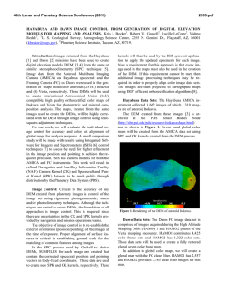
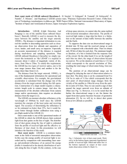
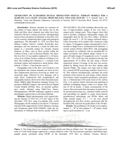
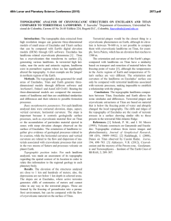
Hydrol. Earth Syst. Sci., 19, 631–643, 2015
www.hydrol-earth-syst-sci.net/19/631/2015/
doi:10.5194/hess-19-631-2015
© Author(s) 2015. CC Attribution 3.0 License.
Assessing the impact of different sources of topographic
data on 1-D hydraulic modelling of floods
A. Md Ali1,2 , D. P. Solomatine1,3 , and G. Di Baldassarre4
1 Department
of Integrated Water System and Knowledge Management, UNESCO-IHE Institute for Water Education,
Delft, the Netherlands
2 Department of Irrigation and Drainage, Kuala Lumpur, Malaysia
3 Water Resource Section, Delft University of Technology, the Netherlands
4 Department of Earth Sciences, Uppsala University, Sweden
Correspondence to: A. Md Ali ([email protected])
Received: 14 May 2014 – Published in Hydrol. Earth Syst. Sci. Discuss.: 3 July 2014
Revised: 16 December 2014 – Accepted: 4 January 2015 – Published: 30 January 2015
Abstract. Topographic data, such as digital elevation models
(DEMs), are essential input in flood inundation modelling.
DEMs can be derived from several sources either through remote sensing techniques (spaceborne or airborne imagery)
or from traditional methods (ground survey). The Advanced
Spaceborne Thermal Emission and Reflection Radiometer
(ASTER), the Shuttle Radar Topography Mission (SRTM),
the light detection and ranging (lidar), and topographic contour maps are some of the most commonly used sources of
data for DEMs. These DEMs are characterized by different
precision and accuracy. On the one hand, the spatial resolution of low-cost DEMs from satellite imagery, such as
ASTER and SRTM, is rather coarse (around 30 to 90 m).
On the other hand, the lidar technique is able to produce
high-resolution DEMs (at around 1 m), but at a much higher
cost. Lastly, contour mapping based on ground survey is time
consuming, particularly for higher scales, and may not be
possible for some remote areas. The use of these different
sources of DEM obviously affects the results of flood inundation models. This paper shows and compares a number of
1-D hydraulic models developed using HEC-RAS as model
code and the aforementioned sources of DEM as geometric
input. To test model selection, the outcomes of the 1-D models were also compared, in terms of flood water levels, to
the results of 2-D models (LISFLOOD-FP). The study was
carried out on a reach of the Johor River, in Malaysia. The
effect of the different sources of DEMs (and different resolutions) was investigated by considering the performance of
the hydraulic models in simulating flood water levels as well
as inundation maps. The outcomes of our study show that
the use of different DEMs has serious implications to the results of hydraulic models. The outcomes also indicate that
the loss of model accuracy due to re-sampling the highest
resolution DEM (i.e. lidar 1 m) to lower resolution is much
less than the loss of model accuracy due to the use of lowcost DEM that have not only a lower resolution, but also a
lower quality. Lastly, to better explore the sensitivity of the
1-D hydraulic models to different DEMs, we performed an
uncertainty analysis based on the GLUE methodology.
1
Introduction
In hydraulic modelling of floods, one of the most fundamental input data is the geometric description of the floodplains
and river channels often provided in the form of digital elevation models (DEMs). During the past decades, there has
been a significant change in data collection for topographic
mapping techniques, from conventional ground survey to remote sensing techniques (i.e. radar wave and laser altimetry;
e.g. Mark and Bates, 2000; Castellarin et al., 2009). This shift
has a number of advantages in terms of processing efficiency,
cost effectiveness and accuracy (Bates, 2012; Di Baldassarre
and Uhlenbrook, 2012).
DEMs can be acquired from many sources of topographic
information ranging from the high-resolution and accurate,
but costly, lidar (Light Detection and Ranging) obtained from
lower altitude, to low-cost, and coarse resolution, spaceborne
Published by Copernicus Publications on behalf of the European Geosciences Union.
632
data, such as ASTER (Advanced Spaceborne Thermal Emission and Reflection Radiometer) and SRTM (Shuttle Radar
Topography Mission). DEMs can also be developed from traditional ground surveying (e.g. topographic contour maps)
by interpolating a number of elevation points.
DEM horizontal resolution, vertical precision and accuracy differ considerably. This diversity is caused by the types
of equipment and methods used in obtaining the topographic
data. When used as an input to hydraulic modelling, the differences in the quality of each DEM subsequently result in
differences in model output performance. In addition, resampling processes of raster data via a geographic information system (GIS) may also deteriorate the accuracy of the
DEMs. The usefulness of diverse topographic data in supporting hydraulic modelling of floods is subject to the availability of DEMs, economic factors and geographical conditions of survey area (Cobby and Mason, 1999; Casas et al.,
2006; Schumann et al., 2008).
To date, a number of studies have been carried out with
the aim of evaluating the impact of accuracy and precision of
the topographic data on the results of hydraulic models (e.g.
Table 1).
Werner (2001) investigated the effect of varying grid element size on flood extent estimation from a 1-D model approach based on a lidar DEM. The study found that the flood
extent estimation increased as the resolution of the DEM becomes coarser.
Horrit and Bates (2001) demonstrated the effects of spatial
resolution on a raster-based flood model simulation. Simulation tests were performed at resolution sizes of 10, 20, 50,
100, 250, 500 and 1000 m and the predictions were compared
with satellite observations of inundated area and ground measurements of flood-wave travel times. They found that the
model reached a maximum performance at resolution of
100 m when calibrated against the observed inundated area.
The resolution of 500 m proved to be adequate for the prediction of water levels. They also highlighted that the predicted
flood-wave travel times are strongly dependent on the model
resolution used.
Wilson and Atkinson (2005) set up a 2-D model,
LISFLOOD-FP, using three different DEMs – contour data
set, synthetic-aperture radar (SAR) data set, and differential
global positioning system (DGPS) – used to predict flood inundation for 1998 flood event in the United Kingdom. The
results showed that the contour data sets resulted in a substantial difference in the timing and the extent of flood inundation when compared to the DGPS data set. Although the
SAR data set also showed differences in the timing and the
extent, it was not as massive as for the contour data set. Nevertheless, the authors also highlighted a potential problem
with the use of satellite remotely sensed topographic data in
flood hazard assessment over small areas.
Casas et al. (2006) investigated the effects of the topographic data sources and resolution on 1-D hydraulic modelling of floods. They found that the contour-based digital terHydrol. Earth Syst. Sci., 19, 631–643, 2015
A. Md Ali et al.: 1-D hydraulic modelling of floods
rain model (DTM) was the least accurate in the determination
of the water level and inundated area of the floodplain; however, the GPS-based DTM led to a more realistic estimate of
the water surface elevation and of the flooded area. The lidarbased model produced the most acceptable results in terms
of water surface elevation and inundated flooded area compared to the reference data. The authors also pointed out that
the different grid sizes used in lidar data have no significant
effect on the determination of the water surface elevation.
In addition, from an analysis of the time–cost ratio for each
DEM used, they concluded that the most cost-effective technique for developing a DEM by means of an acceptable accuracy is from laser altimetry survey (lidar), especially for
large areas.
Schumann et al. (2008) demonstrated the effects of DEMs
on deriving the water stage and inundation area. Three DEMs
at three different resolutions from three sources (lidar, contour and SRTM DEM) were used for a study area in Luxembourg. By using the HEC-RAS 1-D hydraulic model to
simulate the flood propagation, the result shows that the lidar
DEM derived water stages by displaying the lowest RMSE,
followed by the contour DEM and lastly the SRTM. Considering the performance of the SRTM (it was relatively good
with RMSE of 1.07 m), they suggested that the SRTM DEM
is a valuable source for initial vital flood information extraction in large, homogeneous floodplains.
For the large flood-prone area, the availability of DEM
from the public domain (e.g. ASTER, SRTM) makes it easier
to conduct a study. Patro et al. (2009) selected a study area in
India and demonstrated the usefulness of using SRTM DEM
to derive river cross-section for the use in hydraulic modelling. They found that the calibration and validation results
from the hydraulic model performed quite satisfactorily in
simulating the river flow. Furthermore, the model performed
quite well in simulating the peak flow, which is important in
flood modelling. The study by Tarekegn et al. (2010) carried
out on a study area in Ethiopia used a DEM which was generated from ASTER image. Integration between remote sensing and GIS technique were needed to construct the floodplain terrain and channel bathymetry. From the results obtained, they concluded that the ASTER DEM is able to simulate the observed flooding pattern and inundated area extents
with reasonable accuracy. Nevertheless, they also highlighted
the need for advanced GIS processing knowledge when developing a digital representation of the floodplain and channel terrain.
Schumann et al. (2010) demonstrate that near real-time
coarse-resolution radar imagery of a particular flood event
on the River Po (Italy) combined with SRTM terrain height
data leads to a water slope remarkably similar to that derived by combining the radar image with highly accurate airborne laser altimetry. Moreover, they showed that this spaceborne flood wave approximation compares well to a hydraulic model thus allowing the performance of the latter,
www.hydrol-earth-syst-sci.net/19/631/2015/
A. Md Ali et al.: 1-D hydraulic modelling of floods
633
Table 1. Summary of studies assessing the impact of topographic input data on the results of flood inundation models.
Author(s)
Numerical modelling
(1-D*/1-D2-D**/2-D***)
Calibration+ /
validation++ data
Source of DEMs
Type of
assessment
Study area
Horrit and Bates
(2001)
LISFLOODFP**/NCFS**
SAR flood imagery+
Lidar
Precision
River Severn, UK
Werner (2001)
HEC-RAS*
n/a
Laser altimetry data
Precision
River Saar, Germany
Wilson and
Atkinson (2005)
LISFLOOD-FP**
SAR flood
imagery++
InSAR, topography &
GPS
Accuracy
River Nene, UK
Casas et al. (2006)
HEC-RAS*
n/a
GPS, bathymetry, lidar & topography
Accuracy &
precision
River Ter, Spain
Schumann et
al. (2008)
REFIX*** &
HEC-RAS*
Field data+ /1-D
model output++
Lidar, SRTM
topography
Accuracy
River Alzette,
Luxembourg
Schumann et
al. (2010)
HEC-RAS*
Field data+ /lidar
derived water
levels++
Lidar & SRTM
Accuracy
River Po, Italy
Yan et al. (2013)
HEC-RAS*
Field data+ /SAR
flood imagery++
Lidar & SRTM
Accuracy
River Po, Italy
calibrated on a previous event, to be assessed when applied
to an event of different magnitude in near-real time.
Paiva et al. (2011) demonstrated the use of SRTM DEM
in a large-scale hydrologic model with a full 1-D hydrodynamic module to calculate flow propagation on a complex
river network. The study was conducted on one of the major
tributaries of the Amazon, the Purus River basin. They found
that a model validation using discharge and water level data
is capable of reproducing the main hydrological features of
the Purus River basin. Furthermore, realistic floodplain inundation maps were derived from the results of the model. The
authors concluded that it is possible to employ full hydrodynamic models within large-scale hydrological models even
when using limited data for river geometry and floodplain
characterization.
Moya Quiroga et al. (2013) used Monte Carlo simulation
sampling SRTM DEM elevation, and found a considerable
influence of the SRTM uncertainty on the inundation area
(the HEC-RAS hydraulic model of the Timis-Bega Basin in
Romania was employed).
Most recently, Yan et al. (2013) made a comparison between a hydraulic model based on lidar and SRTM DEM.
Besides the DEM inaccuracy, they also introduced uncertainty analysis by considering parameter and inflow uncertainty. The results of this study showed that the differences
between the lidar-based model and the SRTM-based model
are significant, but within the accuracy that is typically associated with large-scale flood studies.
Yet, the aforementioned studies explored the impact of topographic input data on the results flood inundation models
by considering either the accuracy (or quality) or the precision (or resolution) of the DEMs (Table 1). When both accuracy and precision were considered (Casas, 2006), model
www.hydrol-earth-syst-sci.net/19/631/2015/
results were not compared to observations via calibration and
validation exercises.
This paper continues the presented line of research and
deals with the assessment of the effects of using different
DEM data source and resolution in a 1-D hydraulic modelling of floods. The novelty of our study is that both accuracy and precision of the DEM are explicitly considered and
their impacts on hydraulic model results is evaluated in terms
of both water surface elevation and inundation area. Furthermore, we compare model results via independent calibration
and validation exercises and by explicitly considering parameter uncertainty and its potential compensation of inaccuracy
of topographic data.
Hence, the goal of our paper is not to validate a specific
approach for producing flood inundation maps, but rather to
contribute to the existing literature with an original approach
assessing the impact of topographic input data on hydraulic
modelling of floods.
2
2.1
Study area and available data
Study area
The study area is located within the Johor River basin in the
State of Johor, Malaysia. The river basin has a total area of
2690 km2 . The test site is a 30 km reach of the Johor River.
The Johor River channel has a bankfull depth between 5 and
8 m and average slope around 0.03 %. The river reach under study is characterized by a stable main channel from 50
to 250 m wide. The study area consists of agricultural land,
residential and commercial areas (see Fig. 1). As reported
by Department of Irrigation and Drainage, Malaysia (DID,
2009), this test site has been experiencing some major historical flood events since 1948. The most recent ones happened
Hydrol. Earth Syst. Sci., 19, 631–643, 2015
634
A. Md Ali et al.: 1-D hydraulic modelling of floods
in December 2006 and January 2007 when more than 3000
families were evacuated.
2.2
Hydraulic modelling
Flood inundation modelling was carried out by using the
model code HEC-RAS, which was developed by the Hydrologic Engineering Center (HEC) of the United States
Army Corps of Engineers (USACE, 2010). HEC-RAS is a
1-D model that can simulate both steady and unsteady flow
conditions. In this study, all simulations were performed
under unsteady flow conditions. To simulate open channel flows, HEC-RAS numerically solves the full 1-D SaintVenant equations. The HEC-RAS model was set up using
32 cross-sections, whose topography is derived by different DEMs (see below). The observed flow hydrograph at an
hourly time step was used as upstream boundary condition,
while the friction slope was used as downstream boundary
condition. The next section reports the different sources of
topographic data used to define the geometric input. To develop flood inundation maps, the results were post-processed
by using HEC-GeoRAS, an ArcGIS extension.
1-D hydraulic modelling does not properly simulate river
hydraulics and floodplain flows. However, while 2-D models tend to schematize better flood inundation processes, they
do not necessarily perform better when applied to real-world
case studies because, besides model structure, many other
sources of uncertainty affect model results (Werner, 2001;
Bates et al., 2003; Pappenberger et al., 2005; Merwade et al.,
2008; Di Baldassarre et al., 2009, 2010). A number of authors have carried out comparative studies and showed that
the performance of 1-D models is often very close to that of
2-D models (e.g. Horrit and Bates, 2002; Castellarin et al.,
2009; Cook and Merwade, 2009). Also, 1-D models are typically more efficient than 2-D models from a computation
viewpoint, allowing for numerous simulations and uncertainty analysis to be carried out. In our case study, for a given
flow, topography, river reach and a number of simulations, a
HEC-RAS simulation (excluding post-processing GIS) took
only 4 h to predict inundated area, whereas LISFLOOD-FP
took around 26 h.
Anyhow, to properly test our model selection, we carried
out a number of additional experiments (see Sect. 4.2) and
compared the results of 1-D models to the results obtained
with a 2-D model (LISFLOOD-FP; e.g. Hunter et al., 2006;
Bates et al., 2010; Neal et al., 2012; Coulthard et al., 2013).
2.3
Table 2. Information about the eight digital elevation models used
as topographical input.
Model name
DEM type
Jhr L1
Jhr L2
Jhr L20
Jhr L30
Jhr L90
Jhr T20
Jhr A30
Jhr S90
lidar
(rescaled from lidar)
(rescaled from lidar)
(rescaled from lidar)
(rescaled from lidar)
Contour maps
ASTER
SRTM
Resolution (m)
1m
2
20
30
90
20
30
90
1. DEMs derived from an original 1 m lidar data set (obtained from DID).
2. 20 m resolution DEM generated from the vectorial
1 : 25 000 cartography map obtained from DID with a
permission of the Department of Survey and Mapping,
Malaysia (DSMP).
3. 30 m resolution DEM derived from the globally and
freely available ASTER data retrieved from the United
States Geological Survey (USGS, http://earthexplorer.
usgs.gov)
4. 90 m resolution DEM derived from the globally and
freely available SRTM data retrieved from a Consortium
for Spatial Information (CGIAR-CSI, www.cgiar-csi.
org).
To analyse the influence of spatial resolution and separate
it out from the impact of different accuracy, four additional
DEMs were obtained by rescaling the original lidar DEM
(1 m resolution) to the spatial resolutions of the DEMs derived from vectorial cartography (20 m), ASTER (30 m) and
SRTM (90 m). Hence, a total of eight DEMs were used (see
Table 2) to explore the impact of different topographic information on the hydraulic modelling of floods.
Given that the laser/radar waves used in the remote sensing
techniques are not capable of penetrating the water surface
and capture the river bed elevations, all the DEMs were integrated with river cross-section data derived from traditional
ground survey. The ground survey of the river cross-sections
within the study area was systematically carried out at about
1000 m intervals. Then, the flood simulation results across
different data sets were compared to evaluate the effects of
data spatial resolutions and data source differences.
Digital elevation model
The required input data for the HEC-RAS include the geometry of the floodplain and the river, which is provided by
a number of cross-sections. We identified several sources of
DEM data for our study area (details are given below) with
different spatial resolution and accuracy (Fig. 2):
Hydrol. Earth Syst. Sci., 19, 631–643, 2015
3
3.1
Methodology
Evaluating DEM quality
First, the vertical error of each DEM was evaluated through
comparison between the topographic data and 164 GPS
www.hydrol-earth-syst-sci.net/19/631/2015/
A. Md Ali et al.: 1-D hydraulic modelling of floods
635
Figure 1. Layout map of study area: Johor River, Malaysia.
Figure 2. Original DEMs used in this study, based on (a) lidar data, (b) contour map, (c) ASTER data and (d) SRTM data.
ground points taken at random positions within the study
area. The value of each reference elevation point was extracted from the study area using GPS survey equipment. The
quality of each DEM is assessed by the root mean square error (RMSEDEM ) and mean error (MEDEM ). Thus
v
uP
u n
u (ElevGPS − ElevDEM )2
t i=1
RMSEDEM =
,
(1)
n
where ElevGPS is the reference elevation (m) derived from
GPS, ElevDEM is the corresponding value derived from each
DEM, and n corresponds to the total numbers of points.
3.2
for all the models were sampled uniformly from 0.02 to
0.08 m−1/3 s for the river channel, and between 0.03 and
0.10 m−1/3 s for the floodplain, by steps of 0.0025 m−1/3 s.
The performance of the hydraulic models in producing the
observed water levels was assessed by means of the mean
absolute error (MAE):
MAE =
T
1X
|Ot − St | ,
T t=1
(2)
where T is the number of steps in time series, Ot is the observed water level at time t, and St is the simulated water
level at time t.
Model calibration and validation
3.3
Then, data from two recent major flood events that occurred along the Johor River in 2006 and 2007 were used
for independent calibration and validation of the models.
The estimated peak flow of the 2006 event is approximately 375 m3 s−1 , while the one of the 2007 event is around
595 m3 s−1 . Both discharge data were measured and recorded
at Rantau Panjang hydrological station. The 2006 flood data
were used for the calibration exercise, while the 2007 flood
data were used for model validation.
To assess the sensitivity of the different models to the
model parameters, the Manning n roughness coefficients
www.hydrol-earth-syst-sci.net/19/631/2015/
Quantifying the effect of the topographic data
source on the water surface elevation and
inundation area (sensitivity analysis)
The effects of DEM source and spatial resolution were further investigated by examining the sensitivity of model results in terms of maximum water surface elevation (WSE),
inundation area and floodplain boundaries. For this additional analysis, the model results obtained with the most accurate and precise DEM source (lidar at 1 m resolution) were
used as a reference. For WSE analysis, each model was compared to the reference model (Jhr L1, see Table 1) by means
Hydrol. Earth Syst. Sci., 19, 631–643, 2015
636
A. Md Ali et al.: 1-D hydraulic modelling of floods
Table 3. Statistics of errors (m) of each DEMs with respect to the
GPS control points.
Model
name
Jhr L1
Jhr L2
Jhr L20
Jhr L30
Jhr L90
Jhr T20
Jhr A30
Jhr S90
Min.
error (m)
Max.
error (m)
RMSE (m)
−0.59
−0.64
−0.83
−0.93
−5.46
−15.38
−33.37
−3.59
1.00
1.38
1.83
3.98
3.73
10.55
7.58
4.32
0.58
0.58
0.68
0.79
1.27
4.66
7.01
6.47
Reference
Rabus et al. (2003)
Sun et al. (2003)
SRTM mission specification
(Rodríguez et al., 2005)
Berry et al. (2007)
Farr et al. (2007)
Wang et al. (2011)
Figure 3. Comparison between GPS point elevations and elevations
derived by the different DEMs: (a) lidar DEM at different resolution
and (b) different sources of DEMs.
of the following measures:
MADWSE =
x
1X
|WSERef − WSEDEM | ,
x x=1
(3)
(4)
where M1 and M2 are the simulated and observed (i.e. simulated by the reference model) inundation areas, and ∪ and
∩ are the union and intersection GIS operations respectively.
F equal to 100 % indicates that the two areas are completely
coincidental.
3.4
Uncertainty estimation – GLUE analysis
In hydraulic modelling, multiple sources of uncertainty can
emerge from several factors, such as model structure, topography and friction coefficients (Aronica et al., 2002; Trigg
Hydrol. Earth Syst. Sci., 19, 631–643, 2015
Average
height
accuracy (m)
Continent
6.00
11.20
16.00
European
European
Global
3.60
6.20
13.80
Eurasia Global
Eurasia
Eurasia
2.54
et al., 2009; Brandimarte and Di Baldassarre, 2012; Dottori
et al., 2013). A methodological approach to estimate the uncertainty is the generalized likelihood uncertainty estimation
(GLUE) methodology (Beven and Binley, 1992), a variant
of Monte Carlo simulation. Although some aspects of this
methodology are criticized in several papers (e.g. Hunter
et al., 2005; Mantovan and Todini, 2006; Montanari, 2005;
Stedinger et al., 2008), it is still widely used in hydrological modelling because of its ease of implementation and a
common-sense approach to use only a set of the “best” models for uncertainty analysis (e.g. Hunter et al., 2005; Shrestha
et al., 2009; Vázquez et al., 2009; Krueger et al., 2010; Jung
and Merwade, 2012; Brandimarte and Woldeyes, 2013).
According to the GLUE framework (Beven and Binley,
1992), each simulation, i, is associated with the (generalized)
likelihood weight, Wi , ranging from 0 to 1. The weight, Wi
is expressed as a function of the measure fit, εi , of the behavioural models:
Wi =
where WSERef denotes the WSE simulated by the reference
model (Jhr L1), WSEDEM the WSE estimated by the models based on DEMs of lower resolution or different source
(Table 1), and x corresponds to the total number of crosssections where models results where compared.
To analyse the sensitivity to different topographic input in
terms of simulated flood extent, we used the following measure of fit:
M1 ∩ M2
F (%) =
.100,
M1 ∪ M2
Table 4. Reported vertical accuracies of SRTM data.
εmax − εi
,
εmax − εmin
(5)
where εmax and εmin are the maximum and minimum value
of MAE of behavioural models. To identify the behaviour of
the models, a threshold value (rejection criterion) has been
set as follows:
1. simulations associated with MAE larger than 1.0 m and
2. Manning’s n roughness coefficient of the floodplain
smaller than the Manning’s n roughness coefficient of
the channel.
Then, the likelihood weights are the cumulative sum of 1 and
the weighted 5th, 50th and 95th percentiles. The likelihood
weights were calculated as follows:
Li =
Wi
.
n
P
Wi
(6)
i=1
For this study, the applications of uncertainty analysis considered only the parameter uncertainty and implemented for
all DEMs.
www.hydrol-earth-syst-sci.net/19/631/2015/
A. Md Ali et al.: 1-D hydraulic modelling of floods
637
Figure 5. Effect of DEMs on Johor River. Inundation map resulting
from (a) Jhr L1, (b) Jhr L2, (c) Jhr L20, (d) Jhr L30, (e) Jhr L90, (f)
Jhr T20 and (g) Jhr S90.
4
Results and discussion
4.1
Figure 4. Model calibration: contour maps of MAE across the parameter space for (a–h) eight different 1-D models (HEC-RAS) and
(i) for the 2-D model (LISFLOOD-FP).
Table 5. Model validation results.
Model
name
Jhr L1
Jhr L2
Jhr L20
Jhr L30
Jhr L90
Jhr T20
Jhr S90
Jhr LF90
Calibrated Manning’s n
roughness coefficient
Channel
Floodplain
0.0500
0.0450
0.0425
0.0450
0.0450
0.0500
0.0375
0.0550
0.0575
0.0575
0.0575
0.0575
0.0550
0.0750
0.0500
0.0700
MAE (m)
(validation)
0.40
0.38
0.37
0.38
0.39
0.60
0.60
0.52
Quality of DEMs compared with the reference
points
Table 3 shows the calculated statistical vertical errors for
each different DEM for the same study area. As anticipated,
lidar is not only the most precise DEM because of its highest
resolution, but also the most accurate. The RMSE of each lidar DEM increased from 0.58 m (Jhr L1) to 1.27 m (Jhr L90)
as the resolution of the DEMs reduced from 1 m (original
resolution) to 90 m.
Overall, the terrain is considered well defined under the lidar DEMs even though the calculated errors are higher compared to the vertical accuracy reported in product specification (around 0.15 m). Figure 3 shows the distribution of each
DEM compared to the GPS ground elevation.
Although lidar DEM gives the lowest error, it is useful to
note that this type of DEM has a number of limitations as
highlighted in the several papers (see Sun et al., 2003; Casas
et al., 2006; Schumann et al., 2008):
1. it provides only discrete surface height samples and not
continuous coverage,
2. its availability is very much limited by economic constraint,
www.hydrol-earth-syst-sci.net/19/631/2015/
Hydrol. Earth Syst. Sci., 19, 631–643, 2015
638
A. Md Ali et al.: 1-D hydraulic modelling of floods
Table 6. Effects of DEMs (source and resolution) on HEC-RAS
simulations.
Model
name
Jhr L1
Jhr L2
Jhr L20
Jhr L30
Jhr L90
Jhr T20
Jhr S90
Inundation
area (km2 )
Area
difference (%)
F
(%)
F
(%)+
25.86
25.78
25.96
26.18
25.84
29.23
16.58
–
−0.3
0.4
1.2
−0.1
13.0
−35.9
–
96.6
92.9
92.2
89.4
73.7
48.9
–
–
–
–
–
74.2
49.6
Table 7. Summary of mean absolute difference (MAD) in terms of
water surface elevation simulated by the models.
Model name
Jhr L1
Jhr L2
Jhr L20
Jhr L30
Jhr L90
Jhr T20
Jhr S90
MADWSE (m)
–
0.06
0.05
0.05
0.08
1.12
0.76
+ Overlap-fit percentage F (%) of the floodplain inundated area with those
from lidar DEMs of the same resolutions (Jhr L20, Jhr L90).
3. it is unable to capture the river bed elevations due to the
fact the laser does not penetrate the water surface, and
4. it is incapable of penetrating the ground surface in
densely vegetated areas especially for the tropical region.
The RMSE value of the other DEMs is 4.66 m for contour
maps, 7.01 m for ASTER and 6.47 m for SRTM. It is also
noticeable that the RMSE of the SRTM DEM for this particular study area is within the average height accuracy found
in other SRTM literature – either global or at particular continent (see Table 4). Whatever the case, it is proven that this
type of DEM gives an acceptable result when used in largescale flood modelling (e.g. Patro et al., 2009; Paiva et al.,
2012; Yan et al., 2013).
Despite having the lowest vertical accuracies, the ASTER
and contour DEMs are still widely used in the field of hydraulic flood research as they are globally available and free
(e.g. Tarekegn et al., 2010; Wang et al., 2011; Gichamo et
al., 2012). The differences in the vertical accuracies may be
partly due to the lack of information in topographical flats
areas such as floodplains. However, the further use of each
DEM in this study is subject to its performance in the hydraulic flood modelling during the calibration and validation
stages, which are described in the following section.
4.2
Model calibration and validation
Panels (a)–(h) of Fig. 4 show the model responses in terms
of MAE provided by the eight HEC-RAS models in simulating the 2006 flood event. The models were built using the
eight DEMs with different accuracy and precision (Table 2)
as topographic input.
In general, all models (Fig. 4a–h) are seen to be more sensitive to the changing of Manning’s n roughness coefficient
of main channel than the Manning’s n roughness coefficient
of floodplain areas. The results of the calibration showed
that the best-fit models based on lidar DEM with different
resolutions (Jhr L2, Jhr L20, Jhr L30 and Jhr L90) generally gave good performances with only slight variations in
Hydrol. Earth Syst. Sci., 19, 631–643, 2015
the MAE value from 0.38 to 0.41 m. The optimum channel and floodplain Manning’s n roughness coefficient are
centred on similar values at nchannel = 0.0425 to 0.0500 and
nfloodplain = 0.0575 for Jhr L1, Jhr L2, Jhr L20, Jhr L30 and
Jhr L90. The best-fit models based on topographic map and
SRTM also performed well with MAE of 0.31 and 0.50 m.
On the other hand, ASTER-based model completely failed
(the exceptionally high values of MAE in Fig. 4g are due to
model instabilities) and was therefore eliminated from further analysis.
Panel (i) of Fig. 4 shows the outcome of the additional
experiment we carried out to test the appropriateness of selecting a 1-D model. In particular, a LISFLOOD-FP model
was built using the lidar topography rescaled at 90 m, called
here Jhr LF90. The specific topographic input was chosen
as a trade-off between computational times and the need for
an as-accurate-as-possible DEM for a proper comparison between 1-D and 2-D modelling. By comparing the calibration
results of the LISFLOOD-FP model (Fig. 4i) to the corresponding (i.e. using the same topography) ones of the HECRAS model (Fig. 4e), one can observe that differences are
not significant. Lastly, Fig. 4i shows that LISFLOOD-FP is
also more sensitive to the main channel roughness coefficient
than to the floodplain one.
The best-fit models, using the optimum Manning n roughness coefficients (Table 5), were then used to simulate the
January 2007 flood event for model validation. This was carried out for all models except the ASTER-based model due to
its poor performance (see Fig. 4g). Table 5 presents the MAE
of each model obtained during model validation. It is noted
that the MAE values for all lidar-based models (first five
rows) with different resolutions remained almost the same
with the difference within +0.03 m. The MAE values for the
models based on topographic contour maps and SRTM DEM
both provide MAE of 0.60 m.
The model validation exercise also supports the use of 1-D
hydraulic models for this river reach. In particular, Table 5
shows that the LISFLOOD-FP model (Jhr LF90) provided a
MAE of 0.52 m, while the corresponding HEC-RAS model
(Jhr L90) provided a MAE of 0.39 m. Thus, the 1-D model
performed even (slightly) better than the 2-D model.
www.hydrol-earth-syst-sci.net/19/631/2015/
A. Md Ali et al.: 1-D hydraulic modelling of floods
639
Figure 6. Maximum water surface elevation along the Johor River for the six hydraulic models compared to that simulated by the reference
model.
The results of this first analysis suggest that the reduction in the resolution of lidar DEMs (from 1 to 90 m) does
not significantly affect the model performance. However, the
use of topographic contour maps (Jhr T20) and SRTM (Jhr
S90) DEMs as geometric input to the hydraulic model produces a slight increase of model errors. For instance, Jhr L90
and Jhr S90 have the same resolution (90 m), but the different accuracy results in increased (tough not remarkably) errors in model validation (from 0.39 to 0.60 m). This limited
degradation of model performance (Table 5), in spite of the
much lower accuracy of topographic input (Table 2), can be
attributed to the fact that models are compared to water levels
observed in two cross-sections. A spatially distributed analysis (comparing the simulated flood extent and flood water
profile along the river) might show more significant differences (see Sect. 4.3).
www.hydrol-earth-syst-sci.net/19/631/2015/
4.3
4.3.1
Quantifying the effect of the topographic data
source on the water surface elevation and
inundation area on 1-D model
Inundation area (sensitivity analysis)
This section reports an additional analysis aiming to better
explore the sensitivity of model results to different topographic data (see Sect. 3.3). Figure 5 shows the simulated
flood extent maps obtained from the seven different topographic input data. The floodplain areas simulated by the five
lidar-based models (Jhr L1, Jhr L2, Jhr L20, Jhr L30 and Jhr
L90) are very similar. In contrast, the floodplain areas simulated by the models based on topographic contour maps (Jhr
T20) and SRTM DEM (Jhr S90) are substantially different
(see Fig. 5 and Table 6).
Table 6 shows the comparison between the different models in terms of simulating flood extent. The aforementioned
measure of fit F was found to decrease for both decreasing resolution and lowering accuracy. This sensitivity analysis also shows that the results of flood inundation models
are more affected by the accuracy of the DEM used as topographic input than its resolution.
Hydrol. Earth Syst. Sci., 19, 631–643, 2015
640
A. Md Ali et al.: 1-D hydraulic modelling of floods
Figure 7. Comparison of uncertainty bounds (5th, 50th and 95th percentiles by considering parameter uncertainty only) between the reference
model and the other models. The reference model uncertainty bounds are shown as grey areas, while the uncertainty bounds of the other six
models are shown as dashed lines.
4.3.2
Water surface elevation
Figure 6 compares the flood water profiles simulated by the
reference model (Jhr L1) with the flood water profiles (WSE)
obtained from the other six models (Jhr L2, Jhr L20, Jhr L30,
Jhr L90, Jhr T20 and Jhr S90). All these flood water profiles
were obtained by simulating the 2007 flood event. Despite
having different resolutions, the flood water profiles simulated from all lidar-based models portray similar flood water
profiles to the reference model (see Fig. 6a to d). This is consistent with the findings about the inundation area (Fig. 5),
whereas flood water profiles simulated by the models based
on topographic contour maps and SRTM DEMs (see Fig. 6e
and f) are rather different.
The discrepancies between the reference model (Jhr L1)
and the other models as shown in Fig. 6 are quantified in
terms of mean absolute difference (MAD). This shows that
the re-sampled lidar data (Jhr L2, Jhr L20, Jhr L30 and Jhr
L90) all have a low MAD: between 0.05 to 0.08 m. Higher
Hydrol. Earth Syst. Sci., 19, 631–643, 2015
discrepancies are found with the models based on SRTM
DEM (0.76 m) and contour maps (1.12 m). The great differences obtained using the topographic contour maps may be
partly due to the way that the DEM height is sampled. For
instance, the contour DEMs in this study were based on topographic contours at 20 m intervals and required an interpolation technique to generate a DEM. Table 7 shows the MAD
in terms of water surface elevation simulated by the models.
4.3.3
Uncertainty in flood profiles obtained from
different DEMs by considering parameter
uncertainty
To better interpret the differences that have emerged in comparing the results of models based on different topographic
data, we carried out a set of numerical experiments to explore the uncertainty in model parameters. As mentioned,
we varied Manning’s n roughness coefficient between 0.02
and 0.08 m−1/3 s for the river channel, and from 0.03 to
www.hydrol-earth-syst-sci.net/19/631/2015/
A. Md Ali et al.: 1-D hydraulic modelling of floods
0.10 m−1/3 s for the floodplain, in steps of 0.0025 m−1/3 s.
Then a number of simulations were rejected as described in
Sect. 3.4. Figure 7 shows the uncertainty bounds for the different models. The width of these uncertainty bounds was
found to be between 1.5 and 1.6 m for all models (only parameter uncertainty is considered here). Nevertheless, the
model based on contour maps led to significant differences
from the lidar-based model, even when the uncertainty induced by model parameters is explicitly accounted for (see
Fig. 7e).
5
Conclusions
This study assessed how different DEMs (derived by various
sources of topographic information or diverse resolutions) affect the output of hydraulic modelling. A reach of the Johor
River, Malaysia, was used as the test site. The study was performed using a 1-D model (HEC-RAS), which was found
to perform as well as a 2-D model (LISFLOOD-FP) in this
case study. The sources of DEMs were lidar at 1 m resolution, topographic contour maps at 20 m resolution, ASTER
data at 30 m resolution, and SRTM data at 90 m resolution.
The lidar DEM was also re-sampled from its original resolution data set to 2, 20, 30 and 90 m cell size. Different models
were built by using them as geometric input data.
The performance of the five lidar-based models (characterized by different resolutions ranging from 1 to 90 m; see
Table 5) did not show significant differences – neither in the
exercise of independent calibration and validation based on
water level observations in an internal cross-section, nor in
the sensitivity analysis of simulated flood profiles and inundation areas. Another striking result of our study is that the
model based on ASTER data completely failed because of
major inaccuracies of the DEM.
In contrast, the models based on SRTM data and topographic contour maps did relatively well in the validation exercise as they provided a mean absolute error of 0.6 m, which
is only slightly higher than the ones obtained with lidar-based
models (all around 0.4 m). However, this outcome could be
attributed to the fact that validation could only be performed
by using the water level observed in a two internal crosssections. As a matter of fact, higher discrepancies emerged
when lidar-based models were compared to the models based
on SRTM data or topographic contour maps in terms of inundation areas or flood water profiles. These differences were
found to be relevant even when parameter uncertainty was
accounted for.
The study also showed that, to support flood inundation
models, the quality and accuracy of the DEM is more relevant than the resolution and precision of the DEM. For
instance, the model based on the 90 m DEM obtained by
re-sampling the lidar data performed better than the model
based on the 90 m DEM obtained from SRTM data. These
outcomes are unavoidably associated with the specific test
www.hydrol-earth-syst-sci.net/19/631/2015/
641
site, but the methodology proposed here can allow a comprehensive assessment of the impact of diverse topographic data
on hydraulic modelling of floods for different rivers around
the world.
Acknowledgements. The authors would like to thank to the Department of Irrigation and Drainage, Malaysia (DID) for providing
useful input data used in this study. We also acknowledge the Public
Service Department, Malaysia for providing a PhD Fellowship
funding and study leave for the first author. We thank the Editor and
the two anonymous reviewers as well as Fiona, Nagendra, Micah
and Yan for their constructive comments that helped to improve the
manuscript.
Edited by: H. Cloke
References
Aronica, G., Bates, P. D., and Horritt, M. S.: Assessing the uncertainty in distributed model predictions using observed binary pattern information within GLUE, Hydrol. Process., 16, 2001–2016,
doi:10.1002/hyp.398, 2002.
Bates, P. D., Marks, K. J., and Horritt, M. S.: Optimal use of highresolution topographic data in flood inundation models, Hydrol.
Process., 17, 5237–5257, 2003.
Bates, P. D., Horritt, M. S., and Fewtrell, T. J.: A simple inertial
formulation of the shallow water equations for efficient twodimensional flood inundation modelling, J. Hydrol., 387, 33–45,
doi:10.1016/j.jhydrol.2010.03.027, 2010.
Bates, P. D.: Integrating remote sensing data with flood inundation
models: how far have we got?, Hydrol. Process., 26, 2515–2521,
doi:10.1002/hyp.9374, 2012.
Berry, P. A. M., Garlick, J. D., and Smith, R. G.: Near-global validation of the SRTM DEM using satellite radar altimetry, Remote Sens. Environ., 106, 17–27, doi:10.1016/j.rse.2006.07.011,
2007.
Beven, K. and Binley, A.: The future of distributed models – model
calibration and uncertainty prediction, Hydrol. Process., 6, 279–
298, doi:10.1002/hyp.3360060305, 1992.
Brandimarte, L. and Di Baldassarre, G.: Uncertainty in design flood
profiles derived by hydraulic modelling, Hydrol. Res., 43, 753–
761, doi:10.2166/nh.2011.086, 2012.
Brandimarte, L. and Woldeyes, M. K.: Uncertainty in the estimation
of backwater effects at bridge crossings, Hydrol. Process., 27,
1292–1300, doi:10.1002/hyp.9350, 2013.
Casas, A., Benito, G., Thorndycraft, V. R., and Rico, M.: The topographic data source of digital terrain models as a key element in
the accuracy of hydraulic flood modelling, Earth Surf. Process.
Landforms, 31, 444–456, doi:10.1002/esp.1278, 2006.
Castellarin, A., Di Baldassarre, G., Bates, P. D., and Brath, A.:
Optimal cross-section spacing in Preissmann scheme 1-D hydrodynamic models, J. Hydraul. Eng.-ASCE, 135, 96–105,
doi:10.1061/(ASCE)0733-9429(2009)135:2(96), 2009.
Cobby, D. M. and Mason, D. C.: Image processing of airborne scanning laser altimetry for improved river flood modelling, ISPRS J.
Photogramm. Remote Sens., 56, 121–138, 1999.
Hydrol. Earth Syst. Sci., 19, 631–643, 2015
642
Cook, A. and Merwade, V.: Effect of topographic data, geometric
configuration and modeling approach on flood inundation mapping, J. Hydrol., 377, 131–142, 2009.
Coulthard, T. J., Neal, J. C., Bates, P. D., Ramirez, J., de Almeida,
G. A. M., and Hancock, G. R.: Integrating the LISFLOOD-FP 2D
hydrodynamic model with the CAESAR model: implications for
modelling landscape evolution, Earth Surf. Process. Landforms,
38, 1897–1906, doi:10.1002/esp.3478, 2013.
Department of Irrigation and Drainage, Malaysia (DID): Master
plan study on flood mitigation for Johor River basin, Malaysia,
2009.
Di Baldassarre, G., Schumann, G., and Bates, P. D.: A technique
for the calibration of hydraulic models using uncertain satellite
observations of flood extent, J. Hydrol., 367, 276–282, 2009.
Di Baldassarre, G., Schumann, G., Bates, P. D., Freer, J. E., and
Beven, K. J.: Floodplain mapping: a critical discussion on deterministic and probabilistic approaches, Hydrolog. Sci. J., 55,
364–376, 2010.
Di Baldassarre, G. and Uhlenbrook, S.: Is the current flood
of data enough? A treatise on research needs for the improvement of flood modelling, Hydrol. Process., 26, 153–158,
doi:10.1002/hyp.8226, 2012.
Dottori, F., Di Baldassarre, G., and Todini, E.: Detailed data is welcome, but with a pinch of salt: Accuracy, precision, and uncertainty in flood inundation modelling, Water Resour. Res., 49,
6079–6085, doi:10.1002/wrcr.20406, 2013.
Farr, T. G., Rosen, P. A., Caro, E., Crippen, R., Duren, R., Hensley, S., Kobrick, M., Paller, M., Rodriguez, E., Roth, L., Seal, D.,
Shaffer, S., Shimada, J., Umland, J., Werner, M., Oskin, M., Burbank, D., and Alsdorf, D.: The shuttle radar topography mission,
Rev. Geophys., 45, RG2004, doi:10.1029/2005RG000183, 2007.
Gichamo, T. Z., Popescu, I., Jonoski, A., and Solomatine, D.:
River cross-section extraction from the ASTER global DEM
for flood modelling, Environ. Modell. Softw., 31, 37–46,
doi:10.1016/j.envsoft.2011.12.003, 2012.
Horrit, M. S. and Bates, P. D.: Effects of spatial resolution on a
raster based model of flood flow, J. Hydrol., 253, 239–249, 2001.
Horrit, M. S. and Bates, P. D.: Evaluation of 1-D and 2-D models for
predicting river flood inundation, J. Hydrol., 180, 87–99, 2002.
Hunter, N. M., Bates, P. D., Horritt, M. S., De Roo, A. P. J., and
Werner, M. G. F.: Utility of different data types for calibrating flood inundation models within a GLUE framework, Hydrol. Earth Syst. Sci., 9, 412–430, doi:10.5194/hess-9-412-2005,
2005.
Hunter, N. M., Bates, P. D., Horritt, M. S., and Wilson, M. D.: Improved simulation of flood flows using storage cell models, P. I.
Civil Eng.-Wat. M., 159, 9–18, 2006.
Jung, Y. and Merwade, V.: Uncertainty quantification in flood inundation mapping using generalized likelihood uncertainty estimate and sensitivity analysis, J. Hydrol. Eng., 17, 507–520, 2012.
Krueger, T., Freer, J., Quinton, J. N., Macleod, C. J. A., Bilotta, G.
S., Brazier, R. E., Butler, P., and Haygarth, P. M.: Ensemble evaluation of hydrological model hypotheses, Water Resour. Res., 46,
W07516, doi:10.1029/2009WR007845, 2010.
Mantovan, P. and Todini, E.: Hydrological forecasting uncertainty
assessment: incoherence of the GLUE methodology, J. Hydrol.,
330, 368–381, doi:10.1016/j.jhydrol.2006.04.046, 2006.
Hydrol. Earth Syst. Sci., 19, 631–643, 2015
A. Md Ali et al.: 1-D hydraulic modelling of floods
Marks, K. and Bates, P. D.: Integration of high resolution topographic data with floodplain flow models, Hydrol. Process., 14,
2109–2122, 2000.
Merwade, V., Olivera, F., Arabi, M., and Edleman, S.: Uncertainty
in flood inundation mapping: current issues and future directions,
J. Hydrol. Eng., 13, 608–620, 2008.
Montanari, A.: Large sample behaviors of the generalized likelihood uncertainty estimation (GLUE) in assessing the uncertainty
of rainfall-runoff simulations, Water Resour. Res., 41, W08406,
doi:10.1029/2004WR003826, 2005.
Moya Quiroga, V., Popescu, I., Solomatine, D. P., and Bociort, L.: Cloud and cluster computing in uncertainty analysis of integrated flood models, J. Hydroinf., 15, 55–69,
doi:10.2166/hydro.2012.017, 2013.
Neal, J., Schumann, G., and Bates, P.: A subgrid channel model
for simulating river hydraulics and floodplain inundation over
large and data sparse areas, Water Resour. Res., 48, W11506,
doi:10.1029/2012WR012514, 2012.
Paiva, R. C. D., Collischonn, E., and Tucci, C. E. M.: Large
scale hydrologic and hydrodynamic modeling using limited
data and a GIS based approach, J. Hydrol., 406, 170–181,
doi:10.1016/j.jhydrol.2011.06.007, 2011.
Pappenberger, F., Beven, K. J., Horritt, M., and Blazkova, S.: Uncertainty in the calibration of effective roughness parameters in
HEC-RAS using inundation and downstream level observations,
J. Hydrol., 302, 46–69, 2005.
Patro, S., Chatterjee, C., Singh, R., and Raghuwanshi, N. S.:
Hydrodynamic modelling of a large flood-prone system in
India with limited data, Hydrol. Process., 23, 2774–2791,
doi:10.1002/hyp.7375, 2009.
Rabus, B., Eineder, M., Roth, A., and Bamler, R.: The shuttle radar
topography mission – a new class of digital elevation models
acquired by spaceborne radar, ISPRS J. Photogramm. Remote
Sens., 57, 241–262. doi:10.1016/S0924-2716(02)00124-7, 2003.
Rodríguez, E., Morris, C. S., Belz, J. E., Chapin, E. C., Martin, J. M., Daffer, W., and Hensley, S.: An assessment of the
SRTM topographic products, Technical Report JPL D-31639,
Jet Propulsion Laboratory, Pasadena, California, 143 pp., http:
//www2.jplnasa.gov/srtm/srtmBibliography.html (last access: 16
December 2013), 2005.
Schumann, G., Matgen, P., Cutler, M. E. J., Black, A., Hoffmann,
L., and Pfister, L.: Comparison of remotely sensed water stages
from LiDAR, topographic contours and SRTM, ISPRS J. Photogramm. Remote Sens., 63, 283–296, 2008.
Schumann, G., Di Baldassarre, G., Alsdorf, D., and Bates, P. D.:
Near real-time flood wave approximation on large rivers from
space: application to the River Po, Northern Italy, Water Resour.
Res., 46, W05601, doi:10.1029/2008WR007672, 2010.
Shrestha, D. L., Kayastha, N., and Solomatine, D. P.: A novel approach to parameter uncertainty analysis of hydrological models
using neural networks, Hydrol. Earth Syst. Sci., 13, 1235–1248,
doi:10.5194/hess-13-1235-2009, 2009.
Stedinger, J. R., Vogel, R. M., Lee, S. U., and Batchelder,
R.: Appraisal of the generalized likelihood uncertainty estimation (GLUE) method, Water Resour. Res., 44, W00B06,
doi:10.1029/2008WR006822, 2008.
Sun, G., Ranson, K. J., Kharuk, V. I., and Kovacs, K.: Validation of surface height from shuttle radar topography mission us-
www.hydrol-earth-syst-sci.net/19/631/2015/
A. Md Ali et al.: 1-D hydraulic modelling of floods
ing shuttle laser altimetry, Remote Sens. Environ., 88, 401–411.
doi:10.1016/j.rse.2003.09.001, 2003.
Tarekegn, T. H., Haile, A. T., Rientjes, T., Reggiani, P., and
Alkema, D.: Assessment of an ASTER generated DEM for 2D
flood modelling, Int. J. Appl. Earth Obs. Geoinf., 12, 457–465.
doi:10.1016/j.jag.2010.05.007, 2010.
Trigg, M. A., Wilson, M. D., Bates, P. D., Horritt, M. S., Alsdorf,
D. E., Forsberg, B. R., and Vega, M. C.: Amazon flood wave
hydraulics, J. Hydrol., 374, 92–105, 2009.
USACE: HEC-RAS River Analysis System User’s Manual. Version
4.1, Hydrologic Engineering Center, Davis, California, 2010.
Vázquez, R. F., Beven, K., and Feyen, J.: GLUE based assessment
on the overall predictions of a MIKE SHE application, Water
Resour. Res., 23, 1325–1349, doi:10.1007/s11269-008-9329-6,
2009.
www.hydrol-earth-syst-sci.net/19/631/2015/
643
Wang, W., Yang, X., and Yao, T.: Evaluation of ASTER GDEM and
SRTM and their suitability in hydraulic modelling of a glacial
lake outburst flood in southeast Tibet, Hydrol. Process., 26, 213–
225, doi:10.1002/hyp.8127, 2011.
Werner, M. G. F.: Impact of grid size in GIS based flood extent
mapping using a 1-D flow model, Phys. Chem. Earth Pt. B, 26,
517–522, 2001.
Wilson, M. D. and Atkinson, P. M.: The use of elevation
data in flood inundation modelling: a comparison of ERS
interferometric SAR and combined contour and differential GPS data, Intl. J. River Basin Management, 3, 3–20,
doi:10.1080/15715124.2005.9635241, 2005.
Yan, K., Di Baldassarre, G., and Solomatine D. P.: Exploring
the potential of SRTM topographic data for flood inundation modelling under uncertainty, J. Hydroinf., 15, 849–861,
doi:10.2166/hydro.2013.137, 2013.
Hydrol. Earth Syst. Sci., 19, 631–643, 2015