1. Ingeniería

.
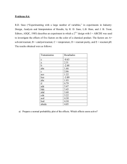
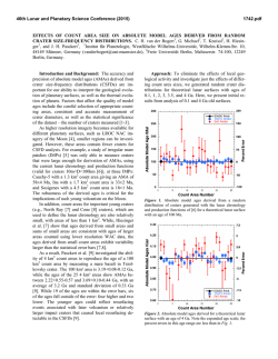
Announcements
Unit
2: Probability
and
distributions
3. Normal distribution
▶ Peer evaluation 1 by Friday 11:59pm
▶ Office hours:
Sta 101 - Spring 2015
– currently MTWR 3-4pm
– propose changing to TR 3-5pm, is this better?
Duke University, Department of Statistical Science
Clicker question
(a) No, keep OH at MTWR 3-4pm
(b) Change to TR 3-5pm
February 2, 2015
Dr. Çetinkaya-Rundel
Slides posted at http://bitly.com/sta101sp15
.
1
.
1. Two types of probability distributions: discrete and continuous
Examples
▶ A discrete probability distribution lists all possible events and the
Discrete:
In a card game if you draw an ace from a
well-shuffled full deck you win $10. If you
draw a red card, you lose $2.
probabilities with which they occur
– The events listed must be disjoint
– Each probability must be between 0 and 1
– The probabilities must total 1
▶ A continuous probability distribution differs from a discrete
probability distribution in several ways:
– The probability that a continuous random variable will equal to any
specific value is zero.
– As such, they cannot be expressed in tabular form.
– Instead, we use an equation or a formula to describe its distribution via a
probability density function (pdf).
– We can calculate the probability for ranges of values the random variable
takes (area under the curve).
.
Outcome
X
P(X)
Win $10 (black aces)
10
2
52
Win $8 (red aces: 10 - 2)
8
2
52
Lose $2 (non-ace reds)
-2
24
52
No win / loss
0
24
52
52
52
2
.
Continuous:
Distribution of weekly
expenditures of entertainment
for a family is right skewed
with median of $70.
=1
3
.
2. Normal distribution is unimodal, symmetric, and follows the 69-95-99.7 rule
Clicker question
Speeds of cars on a highway are normally distributed with mean 65
miles / hour. The minimum speed recorded is 48 miles / hour and the
maximum speed recorded is 83 miles / hour. Which of the following
is most likely to be the standard deviation of the distribution?
N(µ, σ)
▶ Unimodal and symmetric (bell shaped) that follows very strict
guidelines about how variably the data are distributed around
the mean
▶ 68-95-99.7 Rule:
–
–
–
–
(a) -5
about 68% of the distribution falls within 1 SD of the mean
about 95% falls within 2 SD of the mean
about 99.7% falls within 3 SD of the mean
it is possible for observations to fall 4, 5, or more standard deviations
away from the mean, but this is very rare if the data are nearly normal
(b) 5
(c) 10
(d) 15
(e) 30
▶ While most variables are nearly normal, but none are exactly
normal
4
.
5
.
4. Z distribution is normal with µ = 0 and σ = 1
3. Z scores serve as a ruler for any distribution
▶ Linear transformations of normally distributed random variable
Z=
will also be normally distributed.
obs − mean
SD
▶ Hence, if
▶ Z score: number of standard deviations it falls above or below
Z=
the mean
▶ Defined for distributions of any shape, but only when the
X−µ
, where X ∼ N(µ, σ),
σ
then
distribution is normal can we use Z scores to calculate
percentiles
Z ∼ N(0, 1)
▶ Observations with |Z| > 2 are usually considered unusual
▶ Z distribution is a special case of the normal distribution where
µ = 0 and σ = 1 (unit normal distribution)
.
6
.
7
.
Clicker question
Scores on a standardized test are normally distributed with a mean of
100 and a standard deviation of 20. If these scores are converted to
standard normal Z scores, which of the following statements will be
correct?
Application exercise: 2.3 Normal distribution
See the course website for instructions.
(a) The mean will equal 0, but the median cannot be determined.
(b) The mean of the standardized Z-scores will equal 100.
(c) The mean of the standardized Z-scores will equal 5.
(d) Both the mean and median score will equal 0.
(e) A score of 70 is considered unusually low on this test.
8
.
9
.
Anatomy of a normal probability plot
▶ Data are plotted on the y-axis of a normal probability plot, and
Clicker question
theoretical quantiles (following a normal distribution) on the
x-axis
Which of the following is false?
▶ If there is a one-to-one relationship between the data and the
(a) Z scores are helpful for determining how unusual a data point is
compared to the rest of the data in the distribution.
theoretical quantiles, then the data follow a nearly normal
distribution
(b) Majority of Z scores in a right skewed distribution are negative.
▶ Since a one-to-one relationship would appear as a straight line
(c) In a normal distribution, Q1 and Q3 are more than one SD away
from the mean.
on a scatter plot, the closer the points are to a perfect straight
line, the more confident we can be that the data follow the
normal model
(d) Regardless of the shape of the distribution (symmetric vs.
skewed) the Z score of the mean is always 0.
▶ Constructing a normal probability plot requires calculating
percentiles and corresponding Z-scores for each observation,
which is tedious. Therefore we generally rely on software when
making these plots
.
10
.
11
.
Constructing a normal probability plot
Normal probability plot
We construct a normal probability plot for the heights of a sample of
100 men as follows:
A histogram and normal probability plot of a sample of 100 male
heights.
1. Order the observations.
2. Determine the percentile of each observation in the ordered data
set.
●
●
male heights (in.)
●● ● ●
75
●●
●●●●●●●
3. Identify the Z score corresponding to each percentile.
●
●●●●
●
●
●
●
●
●
●
●
●
●
●
●
●
●
●
●
●
●
●
●
●
●
●
●
●
●
●
70
4. Create a scatterplot of the observations (vertical) against the Z
scores (horizontal)
●
●
●
●
●
●
●
●
●
●
●
●
●
●
●
●
●
●
●
●
●
●
●
●
●
●
●
●
●
●
●
●●●●●●
●
●
●
●●●●●
65
●●
● ●●
● ●
Observation i
xi
Percentile , i/(n + 1)
zi
●
60
65
70
75
80
−2
Male heights (inches)
−1
0
1
2
Theoretical Quantiles
Why do the points on the normal probability have jumps?
1
61
0.99%
-2.33
2
63
1.98%
-2.06
3
63
2.97%
-1.89
···
···
···
···
100
78
99.01%
2.33
How are the Z scores corresponding to each percentile determined?
12
.
13
.
6
4
0
0.0
85
0
2
4
6
8
10
−3
−2
−1
0
1
2
3
4
6
Left Skew - Points bend down and to the
right
0.0
2
0.1
0.2
80
0.3
Sample Quantiles
8
0.4
0.5
10
Theoretical Quantiles
75
0
2
4
6
8
10
−3
−2
−1
0
1
2
3
Skinny Tails - S shaped-curve indicating
shorter than normal tails (narrower, less
variable, than expected)
0.2
−1
0
1
2
−2
−1
0
1
0.5
2
−3
−2
−1
0
1
2
3
Theoretical Quantiles
Sample Quantiles
0.20
−4
0.10
0.00
Source: GoDuke.com
Fat Tails - Curve starting below the normal
line, bends to follow it, and ends above it
(wider, more variable, than expected)
6
0.30
8
Theoretical Quantiles
4
−2
2
85
0
80
height (in.)
−2
75
0.0
70
−1.5
0.1
−0.5 0.0
0.3
Sample Quantiles
0.4
1.0
0.5
1.5
Theoretical Quantiles
70
Sample Quantiles
Right Skew - Points bend up and to the left
2
0.1
0.2
0.3
Sample Quantiles
0.4
8
0.5
Below is a histogram and normal probability plot for the heights of
Duke men’s basketball players (from 1990s and 2000s). Do these
data appear to follow a normal distribution?
10
Normal probability plot and skewness
−6
−4
−2
0
2
4
6
8
−3
−2
−1
0
1
2
3
Theoretical Quantiles
.
14
.
15
.
Summary of main ideas
At a pharmaceutical factory the amount of the active ingredient which is
added to each pill is supposed to be 36 mg. The amount of the active
ingredient added follows a nearly normal distribution with a standard
deviation of 0.11 mg. Once every 30 minutes a pill is selected from the
production line, and its composition is measured precisely. We know that
the failure rate of the quality control is 3% at this factory. What are the
bounds of the acceptable amount of the active ingredient?
1. Two types of probability distributions: discrete and continuous
2. Normal distribution is unimodal, symmetric, and follows the
69-95-99.7 rule
3. Z scores serve as a ruler for any distribution
4. Z distribution is normal with µ = 0 and σ = 1
5. Normally distributed data plot as a straight line on the normal
probability plot
.
.
16
.
.
17