1. No category

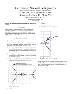
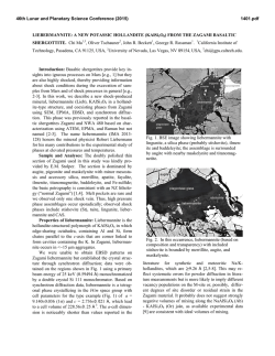
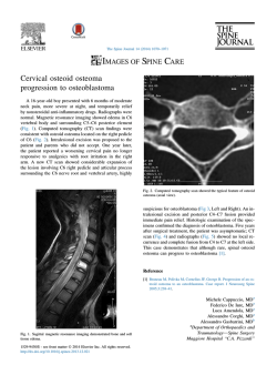
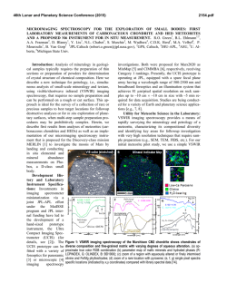
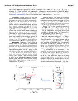
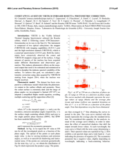
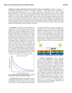
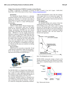
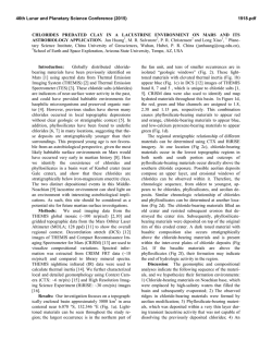
Substitute Exam-EE647-O,Academic Period 2021-1
Solutionary
Jean Estrada Roque
Facultad de Ingeniería Eléctrica y
Electrónica
Universidad Nacional de Ingeniería
Lima, Perú
[email protected]
Abstract—The purpose of this work is to solve the problems
proposed in the substitute exam proposed by engineer Daniel
Carbonel, we will also complement this with simulations that
will make the concepts clearer.
To pass the first and second filter
Keywords—Control theory, root locus, Routh-Hurwitz,
controller, Bode diagram.
Then:
I. PROPOSED EXERCISES
1. The following closed-loop system is shown, you are
asked to determine the value or values that 𝑘 can take, so that
the system is considered stable. (Time: 15 min)
𝐾 + 1 > 0 → 𝐾 > −1
𝐾>0
𝐾>0
Now that we have passed the first and second filters, let's do
the Routh-Hurwitz arrangement
𝑠5
1
2
𝐾+1
𝑠4
1
1
𝐾
3
𝑏1
𝑏2
𝑠2
𝑐1
𝑐2
𝑠
1
𝑑1
𝑠
0
𝑒1
𝑠
Fig. 1. Control system 1
Solution of problem 1
First, we must find the open loop transfer function, for that we
open loop and calculate 𝐺𝐻(𝑠):
We can quickly see that:
𝑐2 = 𝑒1 = 𝐾
Then it would only be necessary to find:
𝑏1, 𝑏2 , 𝑐1 , 𝑑1
Process to find 𝒃𝟏 ∶
Fig. 2. Control system 2
1 1 2
|=1
𝑏1 = − . |
1 1 1
Process to find 𝒃𝟐 ∶
Then:
𝐺𝐻(𝑠) =
𝐾(𝑠 + 1)
𝑠((𝑠 + 1)(𝑠 3 + 1) + 2𝑠 2 )
In advance we know that 𝐾 > 0 because it is open-loop gain.
Remember 1 + 𝐺𝐻(𝑠) = 0 gives you the characteristic
closed-loop equation.
1+
𝐾(𝑠 + 1)
=0
𝑠((𝑠 + 1)(𝑠 3 + 1) + 2𝑠 2 )
1 1 𝐾+1
|=1
𝑏2 = − . |
𝐾
1 1
Process to find 𝒄𝟏 ∶
𝑐1 = −
1 1 1
1
| = − .|
| = 0 → 𝑐1 = 𝜀 > 0
𝑏2
1 1 1
Process to find 𝒅𝟏 ∶
𝑑1 = −
𝑠 5 + 𝑠 4 + 2𝑠 3 + 𝑠 2 + (𝐾 + 1)𝑠 + 𝐾 = 0
1 1
.|
𝑏1 𝑏1
1 𝑏1
.|
𝑐1 𝑐1
1
𝜀 − 𝐾 −𝐾
𝑏2
| = − . |1 1 | =
≈
𝑐2
𝜀 𝜀 𝐾
𝜀
𝜀
Now let's analyze the first column:
Using another online simulator [1], we obtain:
𝑠5
1 (+)
2
𝐾+1
4
1 (+)
1
𝐾
𝑠3
1 (+)
1
2
𝜀 (+)
𝐾
𝑠
𝑠
𝑠1
𝑠0
−𝐾
(−)
𝜀
𝐾 (+)
We notice that there are two sign changes, so I conclude:
∀𝑲 → 𝒔𝒚𝒔𝒕𝒆𝒎 𝒊𝒔 𝒖𝒏𝒔𝒕𝒂𝒃𝒍𝒆
But how do I certify or verify this?
We will simulate in Scilab root locus of 𝐺𝐻(𝑠) using Scilab
console.
Fig. 5. Root Locus 2
Then we see that for every value of 𝑲 the system will always
have poles in the right half plane, and this represents
instability ∀𝑲.
2. There is a 𝑮𝒑(𝒔) plant that is a second order system,
without zeros, whose settling time (for a step input) is 𝑡𝑠 =
1
4 𝑠𝑒𝑐, whose factor damping is
and unity static gain.It is
√10
desired to control said plant, for which a control system is
designed (as shown in the figure below), where the feedback
𝑯(𝒔) is a block represented only by a zero located at -2, with
static gain 0.5 and the 𝑮𝒄(𝒔) block is a “type 2” second order
system, without zeros and with gain static 3.
Fig. 3. Scilab console 1
Note that only 3 command lines were used, this tool is very
useful to certify our calculations, then we get:
Fig. 6. Control system 3
With the above information, you are asked to sketch the
Geometric Place of the Roots for the system presented,
indicating in the drawing the location of the parameters that
you determined for your respective sketch. (Time: 25 min)
Solution of problem 2
Process to find 𝑮𝒑(𝒔) ∶
Fig. 4. Root Locus 1
𝐺𝑝(𝑠) =
𝐾𝑤𝑛2
𝑠 2 + 2𝜀𝑤𝑛 𝑠 + 𝑤𝑛2
𝑡𝑠 = 4 →
𝜀=
1
√10
4
= 4 → 𝜀𝑤𝑛 = 1
𝜀𝑤𝑛
So 𝐺𝐻(𝑠) is:
𝐺𝐻(𝑠) = 𝐺𝑐 (𝑠). 𝐺𝑝(𝑠). 𝐻(𝑠)
→ 𝑤𝑛 = √10
𝐺𝐻(𝑠) =
3
10
(𝑠 + 2)
.
.
𝑠 2 𝑠 2 + 2𝑠 + 10
4
𝐾𝑠𝑠 = 1 → 𝐺𝑝(0) = 1 → 𝐾 = 1
𝐺𝐻(𝑠) =
Then:
𝐺𝑝(𝑠) =
𝑠2
10
+ 2𝑠 + 10
We make
30
4
30(𝑠 + 2)
+ 2𝑠 + 10)
4𝑠 2 (𝑠 2
equal to 𝐾 to find the locus of the roots
Process to find 𝑯(𝒔) ∶
𝐺𝐻(𝑠) =
𝐾(𝑠 + 2)
𝑠 2 (𝑠 2 + 2𝑠 + 10)
𝐻(𝑠) = 𝐾(𝑠 + 2)
Step 1: Number of branches
𝐾𝑠𝑠 =
1
1
1
1
→ 𝐺𝑝(0) = → 𝐾. 2 = → 𝐾 =
2
2
2
4
Then:
#𝑏𝑟𝑎𝑛𝑐ℎ𝑒𝑠 = #𝑝𝑜𝑙𝑒𝑠 𝑜𝑓 𝐺𝐻(𝑠) = 4
Step 2: Existence of locus on the real axis
(𝑠 + 2)
𝐻(𝑠) =
4
We first identify all the poles and zeros of 𝐺𝐻(𝑠) to locate
them in the complex plane and to be able to determine whether
or not there is a locus on the real axis:
Process to find 𝑮𝒄 (𝒔) ∶
𝐺𝑐 (𝑠) =
𝐾
𝑠2
𝑠 = −2 → 𝑟𝑒𝑎𝑙 𝑧𝑒𝑟𝑜
𝑠 = 0 → 𝑟𝑒𝑎𝑙 𝑝𝑜𝑙𝑒 𝑜𝑓 𝑚𝑢𝑙𝑡𝑖𝑝𝑙𝑖𝑐𝑖𝑡𝑦 2
𝑠 = −1 ± 3𝑗 → 𝑐𝑜𝑛𝑗𝑢𝑔𝑎𝑡𝑒𝑑 𝑐𝑜𝑚𝑝𝑙𝑒𝑥 𝑝𝑜𝑙𝑒𝑠
𝐾𝑠𝑠 = 3 → 𝐺𝑝(0) = 3 → 𝐾 = 3
Then:
𝐺𝑐 (𝑠) =
3
𝑠2
We must find the open loop transfer function, for that we open
loop and calculate 𝐺𝐻(𝑠):
Fig. 7. Control system 4
Fig. 8. Root Locus 3
Step 3: Asymptotes
Step 4: Break or bifurcation points (𝝈𝒃 )
a) Number of asymptotes
As GH (s) has the following form:
𝐺𝐻(𝑠) = 𝐾
#𝑎𝑠𝑦𝑚𝑝𝑡𝑜𝑡𝑒𝑠 = #𝑝𝑜𝑙𝑒𝑠 𝑜𝑓 𝐺𝐻(𝑠) − #𝑧𝑒𝑟𝑜𝑠 𝑜𝑓 𝐺𝐻(𝑠)
#𝑎𝑠𝑦𝑚𝑝𝑡𝑜𝑡𝑒𝑠 = 4 − 1 = 3
𝑁(𝑠)
𝐷(𝑠)
From:
1 + 𝐺𝐻(𝑠) = 0 → 1 + 𝐾
b) Convergence point (𝜎𝑐 )
∑ 𝑝𝑜𝑙𝑒𝑠 𝑜𝑓 𝐺𝐻(𝑠) − ∑ 𝑧𝑒𝑟𝑜𝑠 𝑜𝑓 𝐺𝐻(𝑠)
𝜎𝑐 =
#𝑝𝑜𝑙𝑒𝑠 𝑜𝑓 𝐺𝐻(𝑠) − #𝑧𝑒𝑟𝑜𝑠 𝑜𝑓 𝐺𝐻(𝑠)
(−1 + 3𝑗 − 1 − 3𝑗 + 0 + 0) − (−2)
𝜎𝑐 =
4−1
𝜎𝑐 = 0
𝐾=
𝑁(𝑠)
=0
𝐷(𝑠)
−𝐷(𝑠)
𝑁(𝑠)
To find break or bifurcation points:
𝑑𝐾
= 0 → 𝑠 = −3.03 𝑎𝑛𝑑 𝑠 = 0
𝑑𝑠
We discard s = 0, then:
𝜎𝑏 = −3.03
c) Angle with the real axis (𝛽)
Step 5: Intersection with the imaginary axis
From:
(2𝐾 + 1)180°
𝛽=
#𝑝𝑜𝑙𝑒𝑠 𝑜𝑓 𝐺𝐻(𝑠) − #𝑧𝑒𝑟𝑜𝑠 𝑜𝑓 𝐺𝐻(𝑠)
1 + 𝐺𝐻(𝑠) = 0 → 1 +
𝐾(𝑠 + 2)
=0
+ 2𝑠 + 10)
𝑠 2 (𝑠 2
𝑠 4 + 2𝑠 3 + 10𝑠 2 + 𝐾𝑠 + 2𝐾 = 0
Where 𝐾 = 0, 1, 2, … , #𝑎𝑠𝑦𝑚𝑝𝑡𝑜𝑡𝑒𝑠 − 1
Since #𝑎𝑠𝑦𝑚𝑝𝑡𝑜𝑡𝑒𝑠 = 3
(2𝐾 + 1)180°
= (2𝐾 + 1)60°
3
Then 𝐾 = 0, 1, 2
𝛽=
We make 𝑠 = 𝑗𝑤 , and we obtain:
(𝑤 4 − 10𝑤 2 + 2𝐾) + (𝐾𝑤 − 2𝑤 3 )𝑗 = 0 = 0 + 0𝑗
We obtain the following solutions:
𝛽0 = 60°
𝑤 = −√6 𝑎𝑛𝑑 𝐾 = −12
𝛽1 = 180°
𝑤 = 0 𝑎𝑛𝑑 𝐾 = 0
𝛽2 = 300°
𝑤 = √6 𝑎𝑛𝑑 𝐾 = 12
We stay with:
Remember that the 180° asymptote does not exist, so we
discard it.
𝑤 = √6 𝑎𝑛𝑑 𝐾 = 12
Then intersect at:
𝑠 = 𝑗𝑤 = 𝑗√6 = 𝑗2.449 ≈ 𝑗2.45
Fig. 9. Root Locus 4
Fig. 10. Root Locus 5
Step 6: Departure Angle (𝜽𝒅 )
Step 7: Root locus sketch
Due to the presence of complex conjugated poles in GH (s),
the departure angle is calculated, taking a test pole and making
all of them converge to it.
We proceed by sketching according to all the parameters
obtained:
Fig. 13. Root Locus 8
Fig. 11. Root Locus 6
A cleaner graph would be the following:
3
∅1 = tan−1 ( ) = 71.56°
1
3
𝜃1 = 180 − tan−1( ) = 108.435 °
1
𝜃2 = 108.435°
𝜃3 = 90°
∑ ∠𝑝𝑜𝑙𝑒𝑠 = 𝜃1 + 𝜃2 + 𝜃3 = 306.87°
∑ ∠𝑧𝑒𝑟𝑜𝑠 = ∅1 = 71.56°
𝜃𝑑 = 180° − (∑ ∠𝑝𝑜𝑙𝑒𝑠 − ∑ ∠𝑧𝑒𝑟𝑜𝑠)
Fig. 14. Root Locus 9
𝜃𝑑 = −55.31
But how do I certify or verify this?
We will simulate in Scilab the root locus of 𝐺𝐻(𝑠) using
Scilab console.
Fig. 12. Root Locus 7
Fig. 15. Scilab console 2
Note that only 3 command lines were used, this tool is very
useful to certify our calculations, then we get:
Fig. 18. Control system 5
Solution of problem 3
Let's find 𝐺1(𝑠)
𝐾
𝑠
𝐾𝑠𝑠 = 10 → 𝐺𝑝(0) = 𝐾 → 𝐾 = 10
𝐺1(𝑠) =
Then:
𝐺1(𝑠) =
10
𝑠
Then 𝐺𝐻(𝑠):
Fig. 16. Root Locus 10
Using another online simulator [1], we obtain:
𝐺𝐻(𝑠) =
10 10(𝑠 + 0.1)
100(𝑠 + 0.1)
.
=
𝑠 𝑠 2 + 2𝑠 + 2 𝑠(𝑠 2 + 2𝑠 + 2)
We make 100 equal to 𝐾:
𝐺𝐻(𝑠) =
𝐾(𝑠 + 0.1)
𝑠(𝑠 2 + 2𝑠 + 2)
We make 𝑠 = 𝑗𝑤:
𝐺𝐻(𝑗𝑤) =
𝐾(𝑗𝑤 + 0.1)
𝑗𝑤((𝑗𝑤)2 + 2𝑗𝑤 + 2)
Using complex notation:
𝐺𝐻 (𝑗𝑤) =
−𝐾(𝑤 2−1.8)
𝑤 4 +4
−
1.9𝐾(𝑤 2+0.105263)
𝑤(𝑤 4+4)
j
a) Since 𝑃. 𝑀 = 50
𝐹 + 180° = 50° → 𝐹 = −130°
So, I add 180 ° to relocate the angle (F) in the correct quadrant,
to apply the arctangent, so we get 50 °.
Fig. 17. Root Locus 11
3. There is a system like the one shown, where 𝐺1(𝑠) is a firstorder block of type "1", without zeros and with static gain 10,
10(𝑠+0.1)
in addition: 𝐺𝑝(𝑠) = 𝑠2+2𝑠+2 .
−1.9𝐾(𝑤 2 + 0.105263)
𝑤(𝑤 4 + 4)
) = 50°
tan−1 (
−𝐾(𝑤 2 − 1.8)
𝑤4 + 4
Then, we obtain:
𝑤 = −0.6825
You are asked:
a) Calculate the value of K if you want the Phase
Margin to be 50º.
b) What is the value of the gain margin and what can
you say about the stability of the closed-loop system?
(Time: 20 min)
𝑤 = −0.1032
𝑤 = 2.38
We stay with:
𝑤 = 2.38
Evaluating 𝑤 = 2.38 in the magnitude of | 𝐺𝐻 (𝑗𝑤)| , it
would have to give us the value of 1
|
𝐾(𝑗2.38 + 0.1)
|=1
𝑗2.38((𝑗2.38)2 + 2𝑗2.38 + 2)
0.16𝐾 = 1 → 𝐾 = 6.25
How do we certify?
We use Scilab to check if our calculation is right or wrong.
We see that we obtain a phase margin of 27.38 °, which does
not say that our calculation of 𝐾 = 6.25 is not correct, so
what do we do?
We can go testing various values of 𝐾 using the simulator and
precisely for the value of 𝐾 = 2.609 we obtain the desired
phase margin equal to approximately 50 °, obviously we do
this here with the simulator, the idea is that we obtain it
theoretically, so I kindly ask the teacher to upload the
theoretical solution to this problem, for now this
experimental way of finding 𝐾 has been placed since I do not
know how to obtain that value theoretically, however our
simulators can help us for this type of case.
Fig. 19. Scilab console 3
Fig. 21. Scilab console 4
Let's look at the gain and phase margins on the magnitude and
phase bode diagram for 𝐾 = 6.25
We see that we already have the desired phase margin equal
to 50 ° with 𝐾 = 2.609.Let's look at the gain and phase
margins on the magnitude and phase bode diagram for 𝐾 =
2.609
Fig. 20. Bode plot 1
Fig. 22. Bode plot 2
Then , the asked value is 𝑲 = 𝟐. 𝟔𝟎𝟗.
b) Now they ask us to determine the gain margin, now we set
the phase of 𝐺𝐻 (𝑠) to -180, this means that the imaginary
part will be zero, so let's set the imaginary part of 𝐺𝐻 (𝑠) to
zero:
Fig. 24. Root Locus Tool 2
−1.9𝐾(𝑤 2 + 0.105263)
=0
𝑤(𝑤 4 + 4)
𝑤 2 + 0.105263 = 0
We see that there will be no real and positive solutions for 𝑤,
what does this mean? It means that the phase Bode diagram
never touches −180°, so the gain margin is infinite
𝑮. 𝑴 = ∞
Fig. 25. Root Locus Tool 3
What do we conclude about the closed loop system? Since
𝑃. 𝑀 = 50° and 𝑮. 𝑴 = ∞ , then the system will be stable.
OBSERVATIONS
The use of the following online tool [1] is recommended
as it will allow you to check the work done here, it is freely
accessible for educational purposes. This allows you to graph
the locus of the roots and modify the transfer function and
choose different view options.
Fig. 23. Root Locus Tool 1
REFERENCES
[1]
“Drawing
the
root
locus.”
[Online].
Available:
https://lpsa.swarthmore.edu/Root_Locus/RLDraw.html.
[Accessed: 15-Aug-2021].