1. Art and Diseño

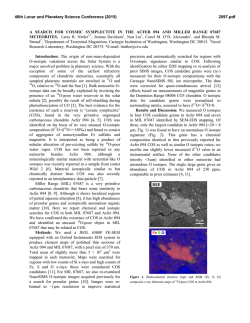
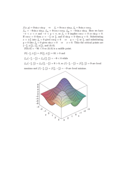
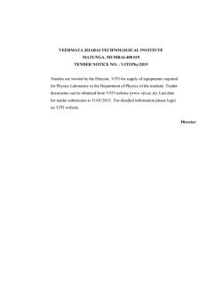
IS GAUSS QUADRATURE BETTER THAN CLENSHAW–CURTIS?
LLOYD N. TREFETHEN∗
Abstract. We consider the question of whether Gauss quadrature, which is very famous, is
more powerful than the much simpler Clenshaw–Curtis quadrature, which is less well-known. Sevenline MATLAB codes are presented that implement both methods, and experiments show that the
supposed factor-of-2 advantage of Gauss quadrature is rarely realized. Theorems are given to explain
this effect. First, following Elliott and O’Hara and Smith in the 1960s, the phenomenon is explained as
a consequence of aliasing of coefficients in Chebyshev expansions. Then another explanation is offered
based on the interpretation of a quadrature formula as a rational approximation of log((z +1)/(z −1))
in the complex plane. Gauss quadrature corresponds to Pad´
e approximation at z = ∞. Clenshaw–
Curtis quadrature corresponds to an approximation whose order of accuracy at z = ∞ is only half
as high, but which is nevertheless equally accurate near [−1, 1].
Key words. Newton–Cotes quadrature, Gauss quadrature, Clenshaw–Curtis quadrature, Chebyshev expansion, rational approximation, FFT, spectral methods
AMS subject classifications. 65D32, 41A20, 41A58
1. Introduction. Every numerical analysis textbook has a chapter on numerical
integration. Most of these present two families of (n + 1)-point quadrature rules: first
Newton–Cotes formulas, based on equally spaced points, and then Gauss formulas,
based on optimal (in a sense) points. Among the books that fit this pattern are
Hamming (1962)
Isaacson and Keller (1966)
Young and Gregory (1972)
Dahlquist and Bj¨
orck (1974)
Burden and Faires (1978)
Stoer and Bulirsch (1980)
Numerical Recipes (1986)
Schwarz and Waldvogel (1989)
Stewart (1996)
Kress (1998)
Plato (2000)
S¨
uli and Mayers (2003)
Henrici (1964)
Acton (1970)
Phillips and Taylor (1973)
Atkinson (1978)
Meinardus and Merz (1979)
Fr¨oberg (1985)
Kahaner, Moler and Nash (1989)
Golub and Ortega (1992)
Tyrtyshnikov (1997)
Van Loan (2000)
Schatzman (2002)
Now in fact, as the books to varying degrees make clear, Newton–Cotes formulas
are useless for high values of n, suffering from the catastrophic O(2n ) Runge phenomenon: they can integrate only functions that are analytic in a large region in the
complex plane, and even these only in the absence of rounding errors [13, 36, 37].
Gauss quadrature formulas, by contrast, have perfect robustness as well as their
well-known apparent factor-of-2 advantage in efficiency: whereas the (n + 1)-point
Newton–Cotes formula exactly integrates polynomials of degree n, the (n + 1)-point
Gauss formula exactly integrates polynomials of degree 2n + 1. Gauss quadrature
nodes and weights take more work to calculate, but this can be done with excellent
accuracy in O(n3 ) operations by solving a tridiagonal eigenvalue problem, as shown
by Golub and Welsch [22]. In the end many of us absorb a simple lesson: for large n,
Gauss quadrature is the only serious competitor.
∗ Oxford Computing Laboratory,
([email protected]).
Wolfson Bldg.,
1
Parks Rd.,
Oxford OX1 3QD, UK
2
L. N. TREFETHEN
This view is mistaken, for Newton–Cotes is a straw man. In fact, we should compare Gauss quadrature with Clenshaw–Curtis quadrature, a much simpler technique
based on sampling the integrand at Chebyshev points. This method also integrates
polynomials of degree n exactly, with no difficulties as n → ∞. Clenshaw–Curtis
formulas are mentioned in the textbooks of Johnson and Riess (1982), Ueberhuber
(1997), Neumaier (2001), and Heath (2002), as well as more briefly in endnotes or exercises in Gautschi (1997) and Cheney and Kincaid (1999). They are not mentioned in
Krylov’s 1962 book on numerical integration [30], but they are treated in later books
in this field including Davis and Rabinowitz (1967, 1975 and 1984), Engels (1980),
and Krommer and Ueberhuber (1998) [10, 13, 14, 29]. Concerning Gauss quadrature,
an indispensable source is the masterful 1981 survey by Gautschi [20].
Perhaps the following is a reasonable summary of the conventional wisdom, among
the minority who are aware of Clenshaw–Curtis quadrature, of n-point quadrature formulas. Gauss quadrature is the gold standard, with perfect convergence and stability
properties, though in some applications one might choose to rely instead on simpler
formulas enhanced by adaptivity or extrapolation. Clenshaw–Curtis is a footnote, for
it is only half as efficient.
We shall see that in fact, for many integrands, Clenshaw–Curtis and Gauss
quadrature are equally efficient.
2. Gauss and Clenshaw–Curtis formulas. Throughout this article we are
concerned with what are known as interpolatory quadrature formulas. A continuous
function f on [−1, 1] is given, and we seek to approximate the integral
(2.1)
I = I(f ) =
Z
1
f (x)dx
−1
by sums
(2.2)
In = In (f ) =
n
X
wk f (xk )
k=0
for various n, where the nodes {xk } depend on n but not f . The weights {wk } are
defined uniquely by the property that In is equal to the integral of the degree ≤ n
polynomial interpolant through the data points. Thus by construction, (2.2) gets the
exactly correct answer if f is a polynomial of degree ≤n.
Newton–Cotes formulas are defined by taking the nodes to be equally spaced
from −1 to 1. The Newton–Cotes formulas of low order are important as building
blocks for discretizations of differential equations and other numerical methods. Their
properties as n → ∞ are very bad, however, and we shall not discuss them further
except for brief reappearances in Figures 2.1 and 6.1.
Gauss formulas are defined by choosing the nodes optimally in the sense of maximizing the degree of polynomials that (2.2) integrates exactly. Since there are n + 1
nodes, it is not surprising that the attainable degree is n + 1 orders higher than in
the generic case, i.e., degree 2n + 1. Gauss quadrature formulas were discovered by
Gauss in his mid-thirties [19], and it is a measure of the extraordinary productivity of
Gauss’s career that this great discovery merits hardly a mention in many accounts of
his life. For these formulas are truly powerful. Their impact was mainly theoretical
before the advent of computers, because of the difficulty of determining the nodes and
weights and also of evaluating integrands at irrational arguments, but in the computer
IS GAUSS QUADRATURE BETTER THAN CLENSHAW–CURTIS?
3
era, especially since the appearance of a paper by Golub and Welsch in 1969 (following earlier work of Goertzel 1954, Wilf 1962 and Gordon 1968), it has been practical
as well [22]. We shall not give details but just offer the following MATLAB function
gauss.m, which is almost the same as the code by the same name in [41].
function I = gauss(f,n)
beta = .5./sqrt(1-(2*(1:n)).^(-2));
T = diag(beta,1) + diag(beta,-1);
[V,D] = eig(T);
x = diag(D); [x,i] = sort(x);
w = 2*V(1,i).^2;
I = w*feval(f,x);
%
%
%
%
%
%
%
(n+1)-pt Gauss quadrature of f
3-term recurrence coeffs
Jacobi matrix
eigenvalue decomposition
nodes (= Legendre points)
weights
the integral
For example, the command gauss(@cos,6) yields 1.68294196961579, which is correct to full precision. The command gauss(@cos,1000) yields the same result, though
it takes 17 seconds on my laptop.1
The idea of Clenshaw–Curtis quadrature is to use Chebyshev points instead of
optimal nodes. There are three main variations on this theme (see [34] for others):
Chebyshev roots in (−1, 1): Fejer’s “first rule” (1933) [15]
Chebyshev extrema in (−1, 1): Fejer’s “second rule” (1933) [15]
Chebyshev extrema in [−1, 1]: Clenshaw and Curtis (1960) [7]
The first and the third variants are also called “classical” and “practical” Clenshaw–
Curtis formulas, respectively. (A number of the relevant papers published especially
in the 1960s make no reference to Fej´er.) It seems that the last choice may be the most
accurate [12] as well as having the easiest connection with the fast Fourier transform,2
and also the potential advantage of convenient reuse of nodes when n is doubled; it
is certainly the one used mainly in practice. The nodes in question, which we shall
simply call Chebyshev points, are defined by
(2.3)
xj = cos
jπ
,
n
0 ≤ j ≤ n.
The Clenshaw–Curtis quadrature formula is the formula (2.2) based on these nodes. A
better name might have been “Chebyshev” or “Fej´er”—indeed, Clenshaw and Curtis
call it “the Chebyshev formula”—but the term Clenshaw–Curtis is standard.
Clenshaw and Curtis published their paper in 1960, before the introduction of the
Fast Fourier Transform in 1965. Soon afterwards, the connection with the FFT was
pointed out by Gentleman [21]. Again we shall not give details but offer a MATLAB
code with the same functionality as gauss.m:
function I = clenshaw_curtis(f,n)
x = cos(pi*(0:n)’/n);
fx = feval(f,x)/(2*n);
g = real(fft(fx([1:n+1 n:-1:2])));
a = [g(1); g(2:n)+g(2*n:-1:n+2); g(n+1)];
w = 0*a’; w(1:2:end) = 2./(1-(0:2:n).^2);
I = w*a;
%
%
%
%
%
%
%
(n+1)-pt C-C quadrature of f
Chebyshev points
f evaluated at these points
fast Fourier transform
Chebyshev coefficients
weight vector
the integral
1 Here are Stroud and Secrest in 1966, working on a Control Data 1604: “The formula for n = 512
took about 4.5 hours to calculate and 0.5 hour to check” [39]. Thus in forty years we have a speedup
from hours on a mainframe to seconds on a laptop.
2 For FFT evaluations of the other two rules, see [44].
4
L. N. TREFETHEN
To get full accuracy for the cosine example, we now need clenshaw_curtis(@cos,11).
Increasing n from 11 to 103 or 106 gives the same result. The former runs in less than
a millisecond on my laptop, and the latter takes 1.6 seconds.
From the point of view of integrating polynomials exactly, Clenshaw–Curtis nodes
appear like Newton–Cotes nodes: both are exact merely for degree n. Yet it is
clear from Figure 2.1 that in a literal sense, at least, they are closer to Gauss
nodes. Certainly they have the same asymptotic distribution as n → ∞, the density
nπ −1 (1 − x2 )−1/2 that is well known to be optimal in various senses for polynomial
approximation on [−1, 1] [41, chap. 5].
Newton−Cotes
Gauss
Clenshaw−Curtis
Fig. 2.1. Newton–Cotes, Gauss, and Clenshaw–Curtis quadrature points in [−1, 1] for n = 32.
The latter two sets have asymptotically the same clustering near ±1 as n → ∞.
3. Experimental comparison. Figure 3.1 shows the convergence as n → ∞ of
the Gauss and Clenshaw–Curtis formulas for six functions f (x). (This experiment is
adapted from Outputs 30b and 30c of [41].) We begin with the monomial f (x) = x20 ,
the algebraic analogue of what in the periodic context would be called a band-limited
function. Here the factor of 2 is in one sense clearly visible: the Gauss formula is
exact for n ≥ 10, the Clenshaw–Curtis formula for n ≥ 20. Even so, it is apparent
that for smaller values of n, the Gauss advantage in efficiency (i.e., size of n needed to
achieve a certain accuracy) is less than a factor of 2. The second function is ex , which
is entire, i.e., analytic throughout the complex plane. Here again Gauss appears more
efficient than Clenshaw–Curtis, but by less than a factor of 2.
Given f ∈ C[−1, 1] and n ≥ 0, let p∗n be the unique best approximation to f on
[−1, 1] of degree ≤ n with respect to the supremum norm k · k = k · k∞ , and define
En∗ = kf − p∗n k. The solid curves in each panel of Figure 3.1 show the errors En∗ and
∗
E2n+1
. (We computed these numbers via Carath´eodory–Fej´er approximation [23]
using the chebfun system [2], a convenient environment for all kinds of explorations
related to this paper.) We shall analyze these curves in the next section, but for now,
we mention just the essential point: Clenshaw–Curtis quadrature converges faster
than En∗ .
2
The next four functions are successively less smooth. The third is e−x , which is
2
also entire, but now with stronger growth O(e|x| ) as x → ∞ in the complex plane.
Here again we see a difference between Gauss and Clenshaw–Curtis quadrature, but
with an efficiency ratio less than 2. The fourth function is f (x) = (1 + 16x2 )−1 ,
which is analytic in a neighborhood of [−1, 1] but not throughout the complex plane,
and now we see that the two quadrature formulas are quite close together. (This
example is discussed further in §6.) For the last two functions, there is again little
difference between Gauss and Clenshaw–Curtis quadrature. We see this both for the
2
C ∞ example e−1/x and for the non-smooth function |x|3 .
These and similar experiments suggest the following conclusions:
5
IS GAUSS QUADRATURE BETTER THAN CLENSHAW–CURTIS?
0
0
10
10
x
20
ex
−5
−5
10
10
−10
−10
10
10
−15
−15
10
10
0
10
20
30
0
0
10
20
30
0
10
10
2
−x
e
2
1/(1+16x )
−5
10
−4
10
−10
10
−15
10
−8
0
10
20
30
0
10
0
10
20
0
10
10
2
3
−1/x
|x|
e
−4
−4
10
10
−8
10
30
−8
0
10
20
30
10
0
10
20
30
Fig. 3.1. Convergence in floating-point arithmetic of Gauss (dots) and Clenshaw–Curtis (circles) quadrature for six functions f on [−1, 1], for n ranging from 1 to 30. The first function is
polynomial, the second and third entire, the fourth analytic, the fifth C ∞ , and the sixth C 2 . The
∗ (upper) and E ∗
solid curves show the minimax approximation errors En
2n+1 (lower).
• As expected, Gauss quadrature matches best degree 2n + 1 polynomial ap∗
proximation: |I − In | ≈ E2n+1
.
• However, Clenshaw–Curtis quadrature does much better than |I − In | ≈ En∗ .
In fact, for functions that are not analytic in a large neighborhood of [−1, 1],
∗
it too comes close to |I − In | ≈ E2n+1
.
• Thus Gauss quadrature significantly outperforms Clenshaw–Curtis quadrature only for functions analytic in a large neighborhood of [−1, 1].
• For such functions, the convergence of both methods is very fast. Thus
Clenshaw–Curtis essentially never requires many more function evaluations
than Gauss to converge to a prescribed accuracy.
We are not the first to observe these surprises. Clenshaw and Curtis themselves
recorded the same effect:
It may be of interest to note that a program based on the proposed
method has been prepared for the Deuce at the National Physical Labo-
6
L. N. TREFETHEN
0
10
|x+0.5|1/2
−4
error
10
−8
10
16
256
4096
65536
n
Fig. 3.2. Convergence of Gauss (dots) and Clenshaw–Curtis (circles) quadrature for the example f (x) = |x + 21 |1/2 of Clenshaw and Curtis, shown on log-log axes. The Gauss formula is applied
only up to n = 210 , since larger values take too much time and memory.
ratory. The upper limit M of the number of terms is 64, and the program
R +1
1
evaluated the integral −1 |x + 12 | 2 dx with an error of 0.00078. This may
be compared with the error of 0.00317 committed by the 32-point Gauss
formula, and of 0.00036 by the 64-point Gauss formula. We see that the
Chebyshev formula, which is much more convenient than the Gauss, may
sometimes nevertheless be of comparable accuracy.
Figure 3.2 examines this function considered by Clenshaw and Curtis for a collection
of values of n. There is no advantage whatever for Gauss quadrature. (The reason
the plot does not match the numbers they report is that it shows data for n = 64
whereas their numbers correspond to n = 63.)
A 1968 paper of O’Hara and Smith makes an unqualified statement [35]:
. . . the Clenshaw–Curtis method gives results nearly as accurate as
Gaussian quadratures for the same number of abscissae.
4. Quadrature, polynomial approximation, and Chebyshev expansions.
How can we explain these observations? In the next section we shall see that some
of the answers can be found in the work in the 1960s of O’Hara and Smith, quoted
above, and Elliott [12]. To prepare the way, we begin with a discussion of some connections between quadrature formulas, polynomial approximations, and Chebyshev
expansions. Though the flavor of these developments is standard, the precise estimates we give are sharper than those we have found in the literature: this applies to
(4.6), (4.10), (4.12), (4.13), and (4.14), as well as the Jackson theorem of footnote 4.
We consider Chebyshev expansions for two reasons: first, because they provide nearbest polynomial approximations and thus near-sharp bounds on Gauss quadrature
errors; second, because they have a special connection with Clenshaw–Curtis quadrature that will lead to an explanation of its surprising accuracy.
Given a continuous function f on [−1, 1], let the degree ≤ n polynomial best
approximation p∗n and error En∗ be defined as in the last section. The rationale for
including the solid curves in Figure 3.1 is the following result due to Bernstein [3].
Theorem 4.1. If the weights wk in (2.2) are nonnegative, as is true for both
IS GAUSS QUADRATURE BETTER THAN CLENSHAW–CURTIS?
7
Gauss and Clenshaw–Curtis quadrature, then for any f ∈ C[−1, 1] and n ≥ 0,
(4.1)
|I − In | ≤ 4En∗ ,
and In → I as n → ∞. In the special case of Gauss quadrature, (4.1) can be improved
to
(4.2)
∗
|I − In | ≤ 4E2n+1
.
Proof. We take advantage of the fact that since (2.2) integrates polynomials of
degree ≤n exactly, I and In are the same for f − p∗n as for f itself. From (2.2), using
the fact that the interval [−1, 1] has length 2, we thus have
|I(f ) − In (f )| = |I(f − p∗n ) − In (f − p∗n )|
(4.3)
≤ |I(f − p∗n )| + |In (f − p∗n )| ≤ 2En∗ +
n
X
k=0
|wk |En∗ .
P
Since the quadrature formula
is interpolatory,
wk = 2, and if the weights are
P
nonnegative, this implies
|wk | = 2, from which (4.1) follows, and similarly (4.2) in
the case of Gauss quadrature since in that case p∗n can be replaced by p∗2n+1 . The
positivity of the weights was proved for Gauss quadrature by Stieltjes in 1884, and
for Clenshaw–Curtis quadrature by Imhof in 1963 [24]. The convergence of In to I is
a consequence of (4.1) together with the Weierstrass approximation theorem.
Theorem 4.1 tells us that if the best approximants to f converge rapidly as n → ∞,
then In will converge rapidly to I. The next step is to combine this theorem with
results of approximation theory to the effect that if f is smooth, its best approximants converge rapidly. We shall consider some results of this kind derived from the
Chebyshev series for a function f ∈ C[−1, 1]. The logic of the development can be
summarized like this:
smooth function f
⇓
rapidly decreasing Chebyshev coefficients
⇓
rapidly converging Chebyshev partial sums
⇓
rapidly converging best approximations
⇓
rapidly converging quadrature
We shall also see that sometimes the sharpest results can be obtained by bypassing steps three and four and going directly from the Chebyshev coefficients to the
quadrature formulas.
Let Tj denote the Chebyshev polynomial of degree j, Tj (x) = cos( j cos−1 x),
which equioscillates between j + 1 extrema ±1 on [−1, 1]. The Chebyshev series for
f ∈ C[−1, 1] is defined by [38, p. 165]
Z
∞
X
2 1 f (x)Tj (x)
′
√
f (x) =
aj Tj (x),
aj =
(4.4)
dx,
π −1
1 − x2
j=0
8
L. N. TREFETHEN
where the prime indicates that the term with j = 0 is multiplied by 1/2. (These
formulas are nothing more than the transplantation to x = cos θ of the Fourier series
for the 2π-periodic even function f (cos θ).) The equals sign in the first formula is
justified, for it is known that the series converges pointwise for any f ∈ C[−1, 1] [31,
p. 119], and if f is H¨older continuous with any H¨older exponent > 0, the convergence
is uniform and absolute [38, p. 168].
Our first step is to show that if f is smooth, its Chebyshev coefficients decrease
rapidly. We consider two smoothness conditions: a kth derivative satisfying a condition related to bounded variation, or analyticity in a neighborhood of [−1, 1]. Regarding the former, let k · kT be the Chebyshev-weighted 1-norm defined by
u′ (x) .
(4.5)
kukT = √
1 − x2 1
This norm is defined via a Stieltjes integral for any u of bounded variation (see, e.g.,
[47, p. 220]), though kukT may be infinite depending on the behavior near x = ±1.
The condition of interest for our theorems is that kf (k) kT should be finite, where f (k)
is the kth derivative of f .3
Theorem 4.2. If f, f ′ , . . . , f (k−1) are absolutely continuous on [−1, 1] and kf (k) kT =
V < ∞ for some k ≥ 0, then for each n ≥ k + 1,
(4.6)
|an | ≤
2V
.
π n(n − 1) · · · (n − k)
If f is analytic with |f (z)| ≤ M in the region bounded by the ellipse with foci ±1 and
major and minor semiaxis lengths summing to ρ > 1, then for each n ≥ 0,
(4.7)
|an | ≤
2M
.
ρn
Proof. For (4.7), see [38, p. 175]. As for (4.6), I do not know where this result
can be found in print; I am grateful to J´ozsef Szabados and Endre S¨
uli for suggesting
the following argument. We proceed by transplanting to the θ = cos−1 x variable and
integrating by parts k + 1 times; the assumptions ensure that the first k derivatives
exist in the ordinary sense√and that f (k) can in turn be written as a Stieltjes integral.
Since dx = − sin θ dθ and 1 − x2 = sin θ, the first integration by parts can be written
as
Z
2 1 f (x)Tn (x)
√
an =
dx
π −1
1 − x2
Z
2 π
f (cos θ) cos(nθ)dθ
=
π 0
Z π
2
=
f ′ (cos θ) sin(nθ) sin θ dθ;
πn 0
the boundary terms vanish because of the sine. The trigonometric identity sin θ1 sin θ2 =
1
1
2 cos(θ1 − θ2 ) − 2 cos(θ1 + θ2 ) converts this to
Z π
2
cos((n − 1)θ) cos((n + 1)θ)
′
an =
f (cos θ)
−
dθ,
πn 0
2
2
3 Our attention to this condition derives from a moral principle: the exponent should come out
right for the function f (x) = |x|. For this function we can take k = 1 in Theorem 4.2, giving
an = O(n−2 ).
IS GAUSS QUADRATURE BETTER THAN CLENSHAW–CURTIS?
9
which implies
cos((n − 1)θ) cos((n + 1)θ) 2
kf ′ (cos θ)k1 −
πn
2
2
∞
cos((n
−
1)θ)
cos((n
+
1)θ)
2
kf ′ (x)kT −
=
πn
2
2
∞
|an | ≤
√
since dθ = dx/ 1 − x2 . The L∞ norm is bounded by 1, and thus we have established
|an | ≤ 2V (0) /πn with V (0) = kf kT . Further integrations by parts bring in higher
derivatives of f and corresponding higher variations up to V (k) = V = kf (k) kT . More
and more cosine terms appear, but the coefficients are such that their sum always has
L∞ norm at most 1. Just as the first integration by parts introduced a factor n in the
denominator, the second leads to factors n − 1 and n + 1, the third to factors n − 2, n,
and n + 2, and so on. To keep the formulas simple we do not keep track of all these
different denominators but weaken the inequality slightly by replacing them all with
n − 1 at the second differentiation, n − 2 at the third, and so on up to n − k at the
(k + 1)st differentiation. The result is (4.6).
Our next step is to consider polynomial approximations obtained as partial sums
of the Chebyshev series. For any n ≥ 0, define
(4.8)
fn (x) =
n
X
′
aj Tj (x)
j=0
and
(4.9)
EnT = kf − fn k ≤
∞
X
j=n+1
|aj |.
(The polynomial fn can be interpreted as the least-squares projection of f onto the
set of polynomials of degree ≤ n with respect to the weight (1 − x2 )−1/2 . It can
also be obtained from f by convolution in the θ variable with a certain n-dependent
kernel [38, p. 166].) The following theorem is a corollary of Theorem 4.2 and equation
(4.9).
Theorem 4.3. If f, f ′ , . . . , f (k−1) are absolutely continuous on [−1, 1] and kf (k) kT =
V < ∞ for some k ≥ 1, then for each n ≥ k + 1,
(4.10)
EnT ≤
2V
.
π k(n − k)k
If f is analytic with |f (z)| ≤ M in the region bounded by the ellipse with foci ±1 and
major and minor semiaxis lengths summing to ρ > 1, then for each n ≥ 0,
(4.11)
EnT ≤
2M
.
(ρ − 1)ρn
Proof. Equation (4.11) follows readily from (4.7) and (4.9). (This bound is
erroneously reported without the factor of 2 on p. 133 of [31].) Similarly, (4.10)
follows from (4.6) and (4.9) if we use the inequality
Z ∞
∞
∞
X
X
1
1
dx
1
≤
≤
=
.
k+1
k+1
j(j − 1) · · · (j − k)
(j − k)
k(n − k)k
n (x − k)
j=n+1
j=n+1
10
L. N. TREFETHEN
Now how does EnT , the error of the truncated Chebyshev series, compare with
the best approximation error En∗ ? In one direction the answer is obvious, since the
optimality of En∗ implies En∗ ≤ EnT .4 In the other direction it is well known that the
gap is never bigger than O(log n). The following theorem states this result together
with another lower bound on En∗ .
Theorem 4.4. For any f ∈ C[−1, 1] and n ≥ 0,
(4.12)
π
|a
| ≤ En∗ ≤ EnT ≤
4 n+1
4
2 + 2 log(2n + 1) En∗ .
π
In particular, EnT < 4.2En∗ for n ≤ 100 and EnT < 7.9En∗ for n ≤ 106 .
Proof. The first inequality is due to Bernstein; see [6, p. 131] or [38, p. 171].
The last inequality follows from the fact that the Lebesgue constant for Chebyshev
projection, which is the same as the Lebesgue constant for Fourier projection defined originally by Lebesgue (1909), is bounded by 1 + (4/π 2 ) log(2n + 1) [18]. The
∼ (4/π 2 ) log n dependence was known already to Fej´er (1910) and Bernstein (1912).
By combining Theorems 4.1 and 4.3, we get bounds on I − In , which Theorem 4.4
indicates are likely to be reasonably sharp. Here are bounds for Gauss quadrature.
Theorem 4.5. Let Gauss quadrature be applied to a function f ∈ C[−1, 1]. If
f, f ′ , . . . , f (k−1) are absolutely continuous on [−1, 1] and kf (k) kT = V < ∞ for some
k ≥ 1, then for each n ≥ k/2,
(4.13)
|I − In | ≤
64V
.
15π k(2n + 1 − k)k
If f is analytic with |f (z)| ≤ M in the region bounded by the ellipse with foci ±1 and
major and minor semiaxis lengths summing to ρ > 1, then for each n ≥ 0,
(4.14)
|I − In | ≤
64M
.
15(ρ − 1)ρ2n+1
Partial proof. Suppose the factors 64/15 in these statements are increased to 8.
Then (4.13) follows from (4.2) and (4.10), and (4.14) from (4.2) and (4.11). The
completion of the proof by sharpening the constants to 64/15 is discussed in the next
section.5
The bounds of Theorem 4.5 are valid for Clenshaw–Curtis quadrature, except
with 2n + 1 replaced by n. However, we do not write these inequalities down, as
we have seen that they are highly pessimistic and our aim is to explain that effect.
Ideally, we would like to establish bounds for Clenshaw–Curtis quadrature that are
not much different from those of Theorem 4.5—i.e., with “2n”, not “n”. The next
section will present such an extension to Clenshaw–Curtis quadrature of (4.13), and
Section 6 will point the way toward a possible extension of (4.14).
4 Thus (4.10) provides a proof of a variant of one of the Jackson theorems of approximation
∗ ≤ 2V /π k(n − k)k .
theory [6, p. 147]: En
5 Bounds based on the assumption of analyticity in an ellipse were first derived by Bernstein [3];
for a discussion, see [20, p. 114]. According to Gautschi, the sharpest result as of 1981 was one
derived by von Sydow, in which 64/15 is replaced in (4.14) by 8ρ/(ρ + 1) [43]. For ρ > 8/7, the
bound (4.14) is better.
11
IS GAUSS QUADRATURE BETTER THAN CLENSHAW–CURTIS?
5. Explanation 1: Chebyshev expansions and aliasing. Let us immediately state our conclusion: the first half of Theorem 4.5 holds for Clenshaw–Curtis as
well as Gauss quadrature. The sole change needed is to replace the condition n ≥ k/2
by the condition of sufficiently large n. Thus Clenshaw–Curtis has essentially the
same algebraic rate of convergence as Gauss quadrature for several-times-differentiable
functions.
Theorem 5.1. Let Clenshaw–Curtis quadrature be applied to a function f ∈
C[−1, 1]. If f, f ′ , . . . , f (k−1) are absolutely continuous on [−1, 1] and kf (k) kT = V <
∞ for some k ≥ 1, then for all sufficiently large n,
(5.1)
|I − In | ≤
64V
.
15π k(2n + 1 − k)k
“Sufficiently large n” means n > nk for some nk that depends on k but not f or V .
Notice the key implication: the factor 2−k in the error bound (4.13) for Gauss
quadrature, which one thinks of as coming from its doubled order of accuracy, applies
to Clenshaw–Curtis quadrature too. In this section we shall derive this bound. The
theorem is new, but it is built on the ideas of Elliott [12] and O’Hara and Smith [35]
forty years ago.
The crucial fact is that of aliasing. Elementary algebra shows that on the grid
in [0, 2π] of 2n equally spaced points θj = πj/n, 0 ≤ j ≤ 2n − 1, the functions
cos((n + p)πθj ) and cos((n − p)πθj ) are indistinguishable for any integer p. We say
that the wave numbers (n + p)π and (n − p)π are aliases of one another on this grid.
Transplanting to the variable x = cos θ gives the following result.
Theorem 5.2. For any integer p with 0 ≤ p ≤ n,
(5.2)
Tn+p (xj ) = Tn−p (xj )
(0 ≤ j ≤ n)
on the Chebyshev grid (2.3). Consequently Clenshaw–Curtis quadrature gives the same
result for both functions,

if n ± p is odd
0
2
(5.3) In (Tn+p ) = In (Tn−p ) = I(Tn−p ) =
,
if n ± p is even

1 − (n − p)2
and the error in integrating Tn+p is

0
8pn
I(Tn+p ) − In (Tn+p ) =
(5.4)
 4
2
n − 2(p + 1)n2 + (p2 − 1)2
if n ± p is odd
if n ± p is even
.
Proof. The equality (5.2) was established by the discussion above it. Since
Clenshaw–Curtis quadrature is exact forR polynomials of degree ≤n, the identity
1
(5.3) follows from the standard formula −1 Tj (x)dx = 2/(1 − j 2 ) for the integral
of a Chebyshev polynomial of even order (which appeared in the penultimate line of
clenshaw_curtis in Section 2). Finally, taking the difference of the integrals with
j = n + p and j = n − p gives (5.4).
From (5.4) we can see why Clenshaw–Curtis quadrature is unexpectedly accurate.
Suppose n is even for simplicity. Then the first few terms in the Chebyshev expansion
of f that contribute to the error I(f ) − In (f ) are
an+2 Tn+2 , an+4 Tn+4 , . . . .
12
L. N. TREFETHEN
However, the exact integrals of these Chebyshev polynomials are small, of order
O(n−2 ), and thanks to aliasing, their values as computed by Clenshaw–Curtis quadrature will also be small. From (5.4), we see that if n is large, the errors associated with
the terms above are approximately
32
16
|a
|,
|a
|, . . . .
n3 n+2 n3 n+4
The numbers grow as the subscript increases from n towards 2n, but even for a
“typical” term an+p , the error will be of order n−2 . For a numerical illustration,
suppose n = 50. Then the (n + 1)-point Clenshaw–Curtis formula integrates T52
inexactly, but the error is only about 0.0001. Similarly its errors for T60 , T70 , T80 ,
and T90 are about 0.0006, 0.002, 0.006, and 0.02, respectively. By contrast the Gauss
formula with n = 50 integrates all the polynomials up to T101 exactly, but after that
its error jumps immediately to order 1: for T102 , about −1.6.
We can now derive (5.1), and in the process, explain how the constant 8 in our
partial proof of Theorem 4.5 can be improved to 64/15.
Proof of Theorem 5.1 and completion of proof of Theorem 4.5. From the Chebyshev expansion of f we know that the quadrature error can be written
I(f ) − In (f ) =
∞
X
′
j=0
aj I(Tj ) − In (Tj ) .
This implies
|I(f ) − In (f )| ≤ S1 + S2 + S3 + S4
where
S1 =
n
X
′
j=0
|aj | I(Tj ) − In (Tj ) ,
2n−⌊n1/3 ⌋
S2 =
X
j=n+1
S3 =
2n+1
X
|aj | I(Tj ) − In (Tj ) ,
j=2n+1−⌊n1/3 ⌋
S4 =
∞
X
j=2n+2
|aj | I(Tj ) − In (Tj ) ,
|aj | I(Tj ) − In (Tj ) .
The term S1 is zero since the
is interpolatory. From (5.4) it
quadrature formula
can be seen that the factors I(Tj ) − In (Tj ) that appear in S2 are all of order at
worst n−2/3 , and by Theorem 4.2, the coefficients aj are of order V n−k−1 . Thus S2
consists of O(n) terms of size O(V n−k−5/3 ), for a total magnitude O(V n−k−2/3 ). The
term S3 consists of O(n1/3 ) terms of size O(V n−k−1 ), for a total magnitude again
O(V n−k−2/3 ). Finally, consider S4 . The partial proof of Theorem 4.5 given in the last
section implies a bound of 8V /πk(2n + 1 − k)k , which is what we would get again now
if we estimated S4 by applying the bound (4.6) for aj together with the inequality
|I(Tj ) − In (Tj )| ≤ 4. However, since j ≥ 4, from (5.2) or (5.3) it can be seen that we
actually have |I(Tj ) − In (Tj )| ≤ 2 + 2/15 = 32/15. It is this observation that sharpens
IS GAUSS QUADRATURE BETTER THAN CLENSHAW–CURTIS?
13
the constant in Theorem 4.5. For Theorem 5.1, we have the freedom to increase n a
little further. In particular, the assumption n ≥ 2 is enough to imply j ≥ 6, further
shrinking the constant to 2 + 2/35 = 72/35. Combining this with (4.6) and putting
the pieces together, we find
S1 + S2 + S3 + S4 ≤ O(V n−k−2/3 ) +
64V /15
144V /35
<
πk(2n + 1 − k)k
πk(2n + 1 − k)k
for large enough n.
6. Explanation 2: rational approximation of log((z + 1)/(z − 1)). So
far, I have not mentioned why this article came to be written. The answer is about
to appear: Figures 6.1 and 6.2. Some time ago I undertook to investigate analogues
for [−1, 1] of observations put forward in [42] about quadrature and rational approximation on (−∞, 0]. As soon as these figures appeared, I knew there was a story to
be told about Clenshaw–Curtis quadrature.
To set the stage, we turn to an old idea for estimating the accuracy of quadrature
formulas applied to analytic functions: Cauchy integrals in the complex plane. As
always, we are interested in the relationship of the integral I of (2.1) to its discrete
approximation In of (2.2) for a function f ∈ C[−1, 1]. Suppose that f is analytic in a
neighborhood of [−1, 1], and let Γ be a contour in the region of analyticity that winds
once around [−1, 1] in the counterclockwise direction. Then using Cauchy’s integral
formula we can write
Z 1
Z 1
Z
Z
1
1
f (z)
f (x)dx =
I =
dz dx =
(6.1)
f (z)φ(z) dz,
2πi Γ
−1 2πi Γ z − x
−1
where φ(z) is given by
(6.2)
φ(z) =
Z
1
−1
z+1
dx
= log
.
z−x
z−1
To be precise, φ is defined as the analytic function in C ∪ {∞}\[−1, 1] given by the
branch of log((z + 1)/(z − 1)) that is positive for z ∈ (1, ∞). At the same time, using
complex residue calculus, we can also express In as a contour integral over Γ:
Z
n
X
1
(6.3)
f (z) rn (z) dz,
wk f (xk ) =
In =
2πi Γ
k=0
where rn is defined by
(6.4)
rn (z) =
n
X
k=0
wk
.
z − xk
Combining (6.1) and (6.3) now gives a beautiful result.
Theorem 6.1. Let f be analytic in a neighborhood of [−1, 1] and let Γ be a
contour contained in the region of analyticity of f that encloses [−1, 1] once in the
counterclockwise direction. Let φ be defined by (6.2), and for any n ≥ 0, let In be the
result of an arbitrary quadrature formula (2.2) with nodes in [−1, 1]. Then the error
is given by
Z
1
(6.5)
f (z)(φ(z) − rn (z)) dz,
I − In =
2πi Γ
14
L. N. TREFETHEN
where rn is defined by (6.4), and hence
(6.6)
|I − In | ≤
1
|Γ| kf kΓ kφ − rn kΓ ,
2π
where |Γ| is the arc length of Γ and k · kΓ is the supremum norm over Γ.
This theorem shows that quadrature over [−1, 1] is associated with a problem in
rational approximation: how closely can φ(z) = log((z + 1)/(z − 1)) be approximated
in a region of the complex plane near [−1, 1] by a rational function of type (n, n + 1),
i.e., with numerator of degree ≤n and denominator of degree ≤ n + 1? Note that
φ(∞) = 0, so it makes sense that the degree of the denominator exceeds that of the
numerator. Any sum (6.4) with nonzero weights wk and distinct nodes xk defines
a rational function of type (n, n + 1), and conversely, if a rational function of type
(n, n + 1) is expanded in partial fractions, it will have the form (6.4) provided it has
n + 1 distinct poles.
The idea of relating quadrature formulas to rational functions goes back to Gauss
himself [19, 20]. In fact, Gauss’s original derivation is closer to this way of thinking
than many of the subsequent developments framed in terms of orthogonal polynomials by Jacobi, Christoffel, Stieltjes and others. Gauss quadrature formulas have a
wonderfully simple characterization in terms of rational approximants:
Theorem 6.2. For any n ≥ 0, the rational function rn of (6.4) associated with
the (n + 1)-point Gauss quadrature formula is the type (n, n + 1) Pad´e approximant
to φ(z) at z = ∞. The function φ − rn has a zero of order exactly 2n + 3 at z = ∞.
Proof. Gauss derived this result by continued fractions [19]; see [20, §1.2].
A Pad´e approximant, as always, is defined as the unique rational function of the
specified type that matches the Taylor expansion of the given function at the given
point, here ∞, to as high an order as possible. This terminology was not available in
Gauss’s day, but Theorem 6.2 is his nonetheless.
What about Clenshaw–Curtis quadrature?
We begin with an experimental comparison. Figure 6.1 shows errors |(φ − rn )(z)|
as contour plots in the complex plane for Newton–Cotes, Gauss, and Clenshaw–Curtis
formulas with n = 8 and 16. In each case the innermost contour corresponds to
|φ(z) − rn (z)| = 1, and moving outward, the levels are 10−1 , 10−2 , . . . , 10−13 . As
z → ∞, all the approximations become very good. Figures like these have been drawn
previously by Takahasi and Mori [40], for Gauss quadrature but not Clenshaw–Curtis,
as part of an important series of papers on quadrature formulas and their enhancement
by changes of variables like the double exponential transformation. Among other
contributions, Takahasi and Mori state Theorem 6.1. The only other publication
that I know of where figures like these appear is [42], for quadrature over (−∞, 0].
What can we infer from such images? Suppose f is analytic in a big region of
the complex plane and does not grow too fast as |z| increases. Then (6.6) implies
that we may get a small bound on |I − In | by integrating over one of the contour
levels far from [−1, 1]. In the extreme case, suppose f is a polynomial of degree k.
Then Theorem 6.2 implies that for Gauss quadrature, (φ − rn )f has a zero of order
2n + 3 − k at ∞. If this number is at least 2, i.e., k ≤ 2n + 1, then by taking circular
contours Γ of radius R → ∞ we get arbitrarily small bounds on I − In , confirming the
exactness of Gauss quadrature for polynomials of degree ≤ 2n + 1. By reversing the
argument we can see that for any interpolatory formula, including Clenshaw–Curtis
or Newton–Cotes, φ − rn must have a zero of order at least n + 2 at ∞. If it did not,
taking a large circular contour Γ in (6.5) would imply a nonzero error I − In for some
monomial f (x) = xk with k ≤ n.
15
IS GAUSS QUADRATURE BETTER THAN CLENSHAW–CURTIS?
Newton−Cotes
n=8
Gauss
n=8
Clenshaw−Curtis
n=8
2
0
−2
−4
−2
0
2
Newton−Cotes
4
n = 16
−4
−2
0
2
Gauss
4
n = 16
−4
−2
0
2
Clenshaw−Curtis
4
n = 16
1
0
−1
−2
−1
0
1
2
−2
−1
0
1
2
−2
−1
0
1
2
Fig. 6.1. Contour plots of the error |φ(z) − rn (z)| for the rational approximations associated
with Newton–Cotes, Gauss, and Clenshaw–Curtis quadrature formulas with n = 8 and 16. The
contours, from inner to outer, correspond to 100 , 10−1 , . . . , 10−13 . The Gauss and Clenshaw–Curtis
errors are virtually identical near [−1, 1], explaining their similar accuracy for functions that are
not analytic in a large region of the plane.
At the other extreme, suppose f is analytic in only a small neighborhood of
[−1, 1]. Then Figure 6.1 suggests that Newton–Cotes quadrature will not converge
at all, which is indeed the case. But the remarkable thing is what it suggests about
Clenshaw–Curtis quadrature. The figure reveals that near [−1, 1], the Clenshaw–
Curtis rational function is essentially indistinguishable from the Gauss rational function as an approximation to φ(z). Thus we can expect that for a function f of this
kind, the two quadrature formulas should have about the same accuracy—exactly
what was observed in the last three sections.
Figure 6.2 shows a closeup for the larger value n = 64. On the left we see contours
for Gauss quadrature, and on the right, Clenshaw–Curtis. Now the pattern is even
more striking. At z = ∞, rn interpolates φ to order 131 for Gauss quadrature and
only order 67 for Clenshaw–Curtis (since n is even, we get one more than the minimal
order n + 2), and that is why the outer curves are twice as far apart on the right as
on the left. The “missing” 64 interpolation points for Clenshaw–Curtis quadrature,
however, lie along a football-shaped curve at a certain distance from [−1, 1] (actually
there are 62 of them, not 64). Inside that curve, the two sides of the figure are almost
indistinguishable.
The following is a first step towards explaining this effect.
Theorem 6.3. Let rn be the rational function (6.4) associated with any interpolatory quadrature formula (2.2) with positive weights. Then the function φ(z) − rn (z)
has at least n + 2 zeros at z = ∞ and exactly 2n + 3 zeros in C ∪ {∞}\[−1, 1] if the
points ±1 are not quadrature nodes, or 2n + 1 zeros if these points are nodes.
Proof. A proof of the assertion about z = ∞ was sketched above. The result
about total count of zeros in C ∪ {∞}\[−1, 1] can be established by applying the
argument principle to φ(z) − r(z) over a contour Γ that encloses [−1, 1] sufficiently
tightly. Each quadrature node in (−1, 1) contributes an decrease in argument by 2π
as Γ passes nearby in the upper half-plane, then another decrease by 2π as it passes
16
L. N. TREFETHEN
Gauss
Clenshaw−Curtis
0.25
0
−0.25
n = 64
−1
−0.5
0
0.5
1
Fig. 6.2. Contour plot of the error |φ(z) − rn (z)| as in Figure 6.1, but for n = 64 and with
Gauss on the left half of the image, Clenshaw–Curtis on the right. The scallops in the curves on
the right reveal the presence of n − 2 finite zeros of φ(z) − r(z) lying along a football-shaped curve
surrounding [−1, 1].
nearby in the lower half-plane, and the final contributions come from φ(z), whose
argument decreases by π near x = 1 and again by π near x = −1. We omit the
details.
Thus we see that all interpolatory quadrature formulas with positive weights
correspond to rational interpolants to φ(z) of order approximately 2n. What distinguishes Gauss quadrature is that all the interpolation takes place at the single point ∞.
The rational functions associated with other quadrature formulas can be interpreted
as examples of what approximation theorists call multipoint Pad´e approximants.
Figure 6.3 explores these interpolation points further, showing the n − 2 zeros of
φ − rn (computed numerically) for four values of n. (When n is odd the number of
finite zeros increases to n − 1 and the number of zeros at z = ∞ shrinks from n + 3 to
n+2.) Two of the interpolation points are real, lying at approximately ±(1+1.8n−2 ),
and the remainder lie in complex conjugate pairs along a curve whose height shrinks
approximately at the rate O(n−1 ). It is an open problem to analyze the details of
this behavior. In particular it would appear that a theorem along the following lines
is likely to be valid, which would make an interesting companion to Theorem 5.1:
the bound (4.14) applies to Clenshaw–Curtis as well as Guass quadrature so long as
n ≤ nρ , where nρ is a number that approaches ∞ as ρ shrinks to 1.
We shall close with an illustration of the implications of Figure 6.3. Consider
again the fourth function of Figure 3.1, f (x) = 1/(1 + 16x2 ). This function is analytic
on [−1, 1] but has poles at ±i/4. In Figure 6.3 we see that the curve of interpolation
points crosses ±i/4 somewhere between n = 32 and n = 64. This suggests that for
values of n larger than about 50, the rate of convergence of the Clenshaw–Curtis
formula will cut in half. To test this prediction, Figure 6.4 extends the earlier computation to n = 120 instead of n = 30. As expected, there is a kink in the convergence
curve at n ≈ 50. Weideman has given an exact analysis of this example [45].
7. Conclusion. Gauss quadrature, one of the jewels of numerical analysis, is
a beautiful and powerful idea. Yet the Clenshaw–Curtis formula has essentially the
same performance and can be implemented effortlessly by the FFT. Figure 6.2 offers
a memorable explanation of the closeness of these two quadrature formulas. The
chebfun system in object-oriented MATLAB takes advantage of the power and speed
of Clenshaw–Curtis quadrature to integrate functions defined by as many as millions
IS GAUSS QUADRATURE BETTER THAN CLENSHAW–CURTIS?
17
1
0.5
n=8
n = 16
n = 32
n = 64
0
−0.5
−1
1
0.5
0
−0.5
−1
−1
−0.5
0
0.5
1
−1
−0.5
0
0.5
1
Fig. 6.3. Points in the complex plane at which φ(z)−rn (z) = 0 for Clenshaw–Curtis quadrature
with n = 8, 16, 32, 64. In addition there are n + 3 interpolation points at z = ∞.
0
10
1/(1+16x2)
−4
10
−8
10
−12
10
−16
10
0
20
40
60
80
100
120
Fig. 6.4. Repetition of the fourth panel of Figure 3.1, but now to the higher value n = 120.
Near n = 50, the rate of convergence cuts abruptly in half as the curve of interpolation points of
Figure 6.3 crosses the poles of f at ±i/4.
of data points [2].
The observations of this paper may have implications for spectral methods for
the numerical solution of ordinary and partial differential equations [4], where the
debate between collocation (≈ Clenshaw–Curtis) and Galerkin (≈ Gauss) methods is
perennial.
Along the way to our Theorem 5.1 on Clenshaw–Curtis quadrature, we have
derived some possibly new results from the consideration of Chebyshev expansions of
smooth functions: on decay of Chebyshev coefficients (see eq. (4.6) and footnote 3), on
near-optimality of truncated Chebyshev series (eqs. (4.10) and (4.12)), on Jacksontype bounds for polynomial best approximations (footnote 4), and on accuracy of
18
L. N. TREFETHEN
Gauss quadrature (eqs. (4.13) and (4.14) and footnote 5).
We hope that others may now take up the challenge of explaining Figures 6.1–6.3
rigorously and establishing corresponding convergence theorems for Clenshaw–Curtis
quadrature, perhaps by making use of the potential theoretic notion of “balayage”.
Acknowledgments. I have benefitted from the advice of Arno Kuijlaars, Alphonse
Magnus, Endre S¨
uli, J´ozsef Szabados, and Andr´e Weideman.
REFERENCES
[1] W. Barrett, Convergence properties of Gaussian quadrature formulae, Comput. J. 3 (1960/61),
272–277.
[2] Z. Battles and L. N. Trefethen, An extension of MATLAB to continuous functions and operators,
SIAM J. Sci. Comp. 25 (2004), 1743–1770.
[3] S. Bernstein, Quelques remarques sur l’interpolation, Math. Ann. 79 (1919), 1–12.
[4] C. Canuto, M. Y. Hussaini, A. Quarteroni and T. A. Zang, Spectral Methods: Fundamentals in
Single Domains, Springer, 2006.
[5] M. M. Chawla, Error estimates for the Clenshaw–Curtis quadrature, Math. Comp. 22 (1968),
651–656.
[6] E. W. Cheney, Introduction to Approximation Theory, McGraw-Hill, 1966.
[7] C. W. Clenshaw and A. R. Curtis, A method for numerical integration on an automatic computer,
Numer. Math. 2 (1960), 197–205.
[8] P. J. Davies, Errors of numerical approximation for analytic functions, in J. Todd, ed., A Survey
of Numerical Analysis, McGraw-Hill, New York, 1962, pp. 468–484.
[9] P. J. Davis and P. Rabinowitz, On the estimation of quadrature errors for analytic functions,
Math. Comp. 8 (1954), 193–203.
[10] P. J. Davis and P. Rabinowitz, Methods of Numerical Integration, Academic Press, New York,
1975.
[11] V. A. Dixon. Numerical quadrature; a survey of the available algorithms, in D. J. Evans, ed.,
Software for Numerical Mathematics, Academic Press, New York, 1974.
[12] D. Elliott, Truncation errors in two Chebyshev series approximations, Math. Comp. 19 (1965),
234–248.
[13] H. Engels, Numerical Quadrature and Cubature, Academic Press, London, 1980.
[14] G. Evans, Practical Numerical Integration, Wiley, Chichester, 1993.
[15] L. Fej´
er, Mechanische Quadraturen mit positiven Cotesschen Zahlen, Math. Z. 37 (1933), 287–
309.
[16] S. Filippi, Angen¨
aherte Tschebyscheff-Approximation einer Stammfunktion—eine Modifikation
des Verfahrens von Clenshaw und Curtis, Numer. Math. 6 (1964), 320–328.
[17] W. Fraser and M. W. Wilson. Remarks on the Clenshaw–Curtis quadrature scheme, SIAM
Review 8 (1966), 322–327.
[18] P. V. Galkin, Estimates for the Lebesgue constants, Proc. Steklov Inst. Math. 109 (1971), 1–4.
[19] C. F. Gauss, Methodus nova integralium valores per approximationem inveniendi, Comment.
Soc. Reg. Scient. Gotting. Recent., 1814 (also in Gauss’s Werke, v. III, pp. 163–196).
[20] W. Gautschi, A survey of Gauss–Christoffel quadrature formulae, in P. L. Butzer and F. Feh´
er,
eds., E. B. Christoffel, Birkh¨
auser, Basel, 1981, pp. 72–147.
[21] W. M. Gentleman. Implementing Clenshaw–Curtis quadrature I and II, Comm. ACM 15 (1972),
337–346, 353.
[22] G. H. Golub and J. H. Welsch, Calculation of Gauss quadrature rules, Math. Comp. 23 (1969),
221–230.
[23] M. H. Gutknecht and L. N. Trefethen, Real polynomial Chebyshev approximation by the
Carath´
eodory–Fej´
er method, SIAM J. Numer. Anal. 19 (1982), 358–371.
[24] J. P. Imhof, On the method for numerical integration of Clenshaw and Curtis, Numer. Math. 5
(1963), 138–141.
[25] D. K. Kahaner, Comparison of numerical quadrature formulas, in J. R. Rice, ed., Mathematical
Software, Academic Press, New York, 1971.
[26] N. S. Kambo, Error bounds for the Clenshaw–Curtis quadrature formulas, BIT 11 (1971), 299–
309.
[27] Y. Katznelson, An Introduction to Harmonic Analysis, Dover, 1976.
[28] M. Kennedy and F. J. Smith, The evaluation of the JWKB phase shift, Mol. Phys. 13 (1967),
443–448.
IS GAUSS QUADRATURE BETTER THAN CLENSHAW–CURTIS?
[29]
[30]
[31]
[32]
[33]
[34]
[35]
[36]
[37]
[38]
[39]
[40]
[41]
[42]
[43]
[44]
[45]
[46]
[47]
19
A. R. Krommer and C. W. Ueberhuber, Computational Integration, SIAM, Philadelphia, 1998.
V. I. Krylov, Approximate Calculation of Integrals, Macmillan, New York, 1962.
J. C. Mason and D. C. Handscomb, Chebyshev Polynomials, Chapman and Hall/CRC, 2003.
J. McNamee, Error-bounds for the evaluation of integrals by the Euler–Maclaurin formula and
by Gauss-type formulae, Math. Comp. 18 (1964), 368–381.
L. P. Natanson, Konstruktive Funktionentheorie, Akademie-Verlag, Berlin, 1955.
S. E. Notaris, Interpolatory quadrature formulae with Chebyshev abscissae, J. Comp. Appl.
Math. 133 (2001), 507–517.
H. O’Hara and F. J. Smith, Error estimation in the Clenshaw–Curtis quadrature formula, Computer J. 11 (1968), 213–219.
J. Ouspensky, Sur les valeurs asymptotiques des coefficients de Cotes, Bull. Amer. Math. Soc.
31 (1925), 145–156.
¨
G. P´
olya, Uber
die Konvergenz von Quadraturverfahren, Math. Z. 37 (1933), 264–286.
T. J. Rivlin, Chebyshev Polynomials: From Approximation Theory to Algebra and Number
Theory, 2nd ed., Wiley, 1990.
A. H. Stroud and D. Secrest, Gaussian Quadrature Formulas, Prentice-Hall, 1966.
H. Takahasi and M. Mori, Estimation of errors in the numerical quadrature of analytic functions,
Applicable Anal. 1 (1971), 201–229.
L. N. Trefethen, Spectral Methods in MATLAB, SIAM, Philadelphia, 2000.
L. N. Trefethen, J. A. C. Weideman, and T. Schmelzer, Talbot quadratures and rational approximations, BIT, to appear.
B. von Sydow, Error estimates for Gaussian quadrature formulae, Numer. Math. 29 (1977),
59–64.
J. Waldvogel, Fast construction of the Fej´
er and Clenshaw–Curtis quadrature rules, BIT 46
(2006), 195–202.
J. A. C. Weideman, Explicit error formulas for interpolatory quadrature rules for rational integrands, manuscript, 2006.
K. Wright, Series methods for integration, Computer J. 9 (1966), 191–199.
W. P. Ziemer, Weakly Differentiable Functions, Springer, 1989.