
1 - arXiv
arXiv:1502.00422v1 [math.DS] 2 Feb 2015
THE ERROR TERM OF THE PRIME ORBIT THEOREM
FOR EXPANDING SEMIFLOWS
MASATO TSUJII
Abstract. We consider suspension semiflows of an angle multiplying map on
the circle and study the distributions of periods of their periodic orbits. Under
generic conditions on the roof function, we give an asymptotic formula on the
number π(T ) of prime periodic orbits with period ≤ T . The error term is
bounded, at least, by
1
exp
1−
+ ε htop T
in the limit T → ∞
4⌈χmax /htop ⌉
for arbitrarily small ε > 0, where htop and χmax are respectively the topological entropy and the maximal Lyapunov exponent of the semiflow.
1. Introduction
t
For a flow f : M → M on a closed manifold M with some hyperbolicity, it
is well known that the number π(T ) of periodic orbits with period ≤ T grows
exponentially as T → ∞ and the exponential rate coincides with the topological
entropy htop of the flow. The prime orbit theorem, due to Parry and Pollicott[6,
Theorem 9.3], gives a more precise estimate in the case of topologically weakly
mixing hyperbolic flows:
Z T htop t
e
(1)
π(T ) = (1 + o(1))
dt as T → ∞.
t
1
This paper addresses estimates of the error term in this asymptotic formula.
For geodesic flows on surfaces with negative (variable) curvature, Pollicott and
Sharp[8] proved that the relative error term, denoted by o(1) in the formula (1)
above, is actually exponentially small, that is, bounded by Ce−εT with some C > 0
and ε > 0. More recently, this result is extended to the higher dimensional cases
by Giulietti, Liverani and Pollicott[3] and Stoyanov[10]. But not much is known
about the exponential rate at which the relative error term decreases.
For the geodesic flows on surfaces with negative constant curvature, we have a
much more precise asymptotic formula due to Huber, which reads
Z T htop t
k Z T µi t
X
e
e
dt +
dt + O eρt
(2)
π(T ) =
t
t
1
i=1 1
where ρ = (3/4)htop and µi , 1 ≤ i ≤ k, are real numbers satisfying ρ < µi < htop .
(The exponents µi correspond to small eigenvalues of the Laplacian on the surface.
See [2].) But this result is known only for the case of constant curvature because
the proof is based on the fact that the geodesic flow in such case is identified with
Date: February 3, 2015.
1
2
MASATO TSUJII
the action of a hyperbolic one-parameter subgroup of SL(2, R) on its quotient space
by a discrete subgroup.
Comparing the results mentioned above, we are tempted to pose a question
whether such a precise asymptotic formula as (2) is available for more general type
of hyperbolic flows and by a more flexible method. In this paper, we pursue this
question in the case of the suspension semiflows of an angle multiplying map on the
circle and provide a positive answer under generic conditions on the roof function.
2. The main results
2.1. Definitions. We consider a class of (simplest possible) expanding semiflows.
This kind of semiflows have been studied in [9, 7, 11] as a simplified model of Anosov
flows. First we fix a positive integer ℓ ≥ 2 and consider the angle-multiplying map
τ : S1 → S1,
τ (x) = ℓx
mod Z.
∞
Let C+
(S 1 ) be the space of positive-valued C ∞ functions on S 1 . Then we consider
∞
the suspension semiflow of τ with roof function f ∈ C+
(S 1 ):
Tf = {Tft : Xf → Xf | t ≥ 0}.
(See Figure 1.) This is a semiflow on the set
Xf := {(x, y) ∈ S 1 × R | 0 ≤ y < f (x)} ⊂ S 1 × R
and defined precisely by the expression
Tft (x, y) = (τ n(x,y+t;f ) (x), y + t − f (n(x,y+t;f ))(x))
where
(3)
f (n) (x) =
n−1
X
f (τ i (x))
i=0
and
(4)
n(x, t; f ) = max{n ≥ 0 | f (n) (x) ≤ t}.
2.2. Spectral properties of transfer operators. By a heuristic argument, the
distribution of periods of periodic orbits of Tf is related to the spectra of the
transfer operators
X
Lt ϕ(z) =
ϕ(w).
w:Tft (w)=z
Indeed, computing the flat trace of Lt , defined as the integral of the Schwartz kernel
K t (z, w) of Lt along the diagonal z = w, we find
Tr ♭ Lt =
∞
XX
|γ|
· δ(t − n|γ|)
1 − Eγ−n
γ∈Γ n=1
where Γ is the set of prime periodic orbits and |γ| and Eγ denote respectively the
prime period and the (coefficient of) linearized Poincar´e map. If we ignore the sum
THE ERROR TERM OF THE PRIME ORBIT THEOREM
3
Xf
x
τ (x)
Figure 1. Expanding semiflow Tf
over n ≥ 2 and also the term Eγ−n in the denominator of the summands (which are
in fact relatively small), we would have
Z T
X
1
1
♭ t
· Tr L ∼
· Tr ♭ Lt dt ∼ π(T ).
δ(t − |γ|),
and so
t
1 t
γ∈Γ
Therefore, if the flat trace Tr ♭ Lt were related to the spectrum of Lt as in the case
of the usual trace, the asymptotics of π(T ) would be expressed in terms of the
spectrum of Lt . For this reason, we are going to study the spectral properties of
the transfer operators Lt .
Let us say that a function ϕ : Xf → C is of class C ∞ if Lt ϕ for t ≥ 0 are
∞
C functions on the interior Xf◦ of Xf (as a subset of S 1 × R) and each of their
partial derivatives are bounded. Let C ∞ (Xf ) be the space of C ∞ functions on Xf
an d suppose that it is equipped with the C ∞ topology induced by the uniform C r
norms kϕ|Xf◦ kC r for r ≥ 0. With this definition, we may regard Lt for t ≥ 0 as a
continuous operator
Lt : C ∞ (Xf ) → C ∞ (Xf ).
To study spectral properties of Lt , we will define Banach spaces
C ∞ (Xf ) ⊂ B r,p (Xf ) ⊂ L2 (Xf )
for real numbers r > 0 and integers p ≥ 1 and consider the natural extensions of Lt
to them. The next theorem gives a spectral property of Lt on B r,p (Xf ) under some
generic conditions on the roof function f . We write h(f ), χmax (f ) and χmin (f )
respectively for the topological entropy, the maximum Lyapunov exponent and the
minimum Lyapunov exponent:
χmax (f ) := lim
t→∞
1
max log kDTft (z)k,
t z∈Xf
χmin (f ) := lim
t→∞
1
min log kDTft (z)k.
t z∈Xf
4
MASATO TSUJII
We put
α(f ) :=
χmax (f )
.
h(f )
We always have α(f ) ≥ 1 from Ruelle inequality[4] and may regard α(f ) as a
measurement of spacial non-uniformity of expansion by the semiflow Tf .
∞
Theorem 2.1. For any f ∈ C+
(S 1 ), any r > 0 and any integer p ≥ 1, the transfer
t
operators L for sufficiently large t > 0 extend to bounded operators
Lt : B r,p (Xf ) → B r,p (Xf ).
(5)
For each integer p ≥ 1 and for each ε > 0, there exists an open and dense
∞
subset Up (ε) ⊂ C+
(S 1 ) such that, if f ∈ Up (ε) and if r > 0 is so large that
r > χmax (f )/χmin (f ), the essential spectral radius of the operator (5) for sufficiently large t > 0 is smaller than exp((ρp (f ) + ε)t) where
1
max {p, α(f )} − 1
(6)
ρp (f ) :=
1+
· h(f ).
2
p
Remark 2.2. The conclusion of the theorem above implies that the spectral set of
(5) on the region |z| ≥ exp((ρp (f ) + ε)t) consists of finitely many eigenvalues with
finite multiplicities. Such eigenvalues (counted with multiplicity) are written in the
form exp(µi t), i = 1, 2, · · · , I, for complex numbers µi that do not depend on t.
(See [11, pp295].)
The case p = 1 in the theorem above corresponds to the result in our previous
paper [11], where the bound is
ρ1 (f ) = exp(χmax (f ) · t/2)
as α(f ) ≥ 1. (See also [12, 13] for the corresponding results for contact Anosov
flows.) This bound is preferable when α(f ) is close to 1, but the claim becomes
vacuous when α(f ) ≥ 2 for ρ1 (f ) exceeds the topological entropy htop (f ). The
improvement achieved in Theorem 2.1 is that we get better bounds by choosing
different integers p ≥ 1 depending on α(f ) ≥ 1. For simplicity’s sake, suppose that
∞
1
f belongs to the residual subset U := ∩p∈N ∩∞
m=1 Up (1/m) ⊂ C+ (S ) and set
ρ(f ) := min ρp (f ).
p≥1
So, letting
(7)
1
p(f ) = ⌈α(f )⌉ ≥ 1, we have
ρ(f ) ≤ ρp(f ) (f ) ≤ 1 −
1
2p(f )
h(f ) < h(f ).
That is, by choosing suitable p ≥ 1, we always get a bound for the essential spectral
radius of Lt that is strictly smaller than the spectral radius exp(h(f )t) .
2.3. Asymptotics of the number of periodic orbits. We next give a consequence of Theorem 2.1 on the remainder term of the prime orbit theorem. Let
Γ = Γ(f ) be the set of prime periodic orbits for the semi flow Tf . For a prime
periodic orbit γ ∈ Γ, we denote its period by |γ|. Let π(T ) = #{γ ∈ Γ | |γ| ≤ T }.
1This choice of p is not always optimal.
THE ERROR TERM OF THE PRIME ORBIT THEOREM
5
∞
Theorem 2.3. Let ε > 0 and suppose that the roof function f ∈ C+
(S 1 ) belongs
∞
to the open and dense subset Up (ε) ⊂ C+ (Xf ) given in Theorem 2.1 for p ≥ 1.
Then, with setting
(8)
ρ¯ = ρ¯p (f ) :=
ρp (f ) + h(f )
,
2
we have an asymptotic formula
Z T htop t
I Z T µi t
X
e
e
¯
,
π(T ) =
dt +
dt + O e(ρ+ε)t
t
t
1
i=1 1
where µi , 1 ≤ i ≤ I ′ , are complex numbers satisfying ρ¯ + ε < ℜ(µi ) < h(f ).
Remark 2.4. µi above are those in Remark 2.2 satisfying ρ¯ + ε < ℜ(µi ) < h(f ).
Remark 2.5. If we let p = p(f ) = ⌈α(f )⌉ ≥ 1, we have, from (7), that
1
ρ¯p (f ) ≤ 1 −
h(f ) < h(f ).
4⌈χmax (f )/h(f )⌉
3. The generic condition
We set up notation on the dynamics of the semiflow Tf and formulate the
transversality condition that defines the open dense subset Up (ε) in Theorem 2.1.
3.1. Differential of the semiflow Tf . The differential DTft (z) : R2 → R2 at
z ∈ Xf is well-defined if z and Tft (z) are not on the (lower) boundary of Xf . In
general, we define
DTft (z) = lim DTft (x, y + ε) : R2 → R2 ,
ε→+0
DTft (x, y
where
+ ε) for sufficiently small ε > 0 is constant and hence the limit on
the right hand side is well-defined. For t ≥ 0, we set
E(z, t; f ) = ℓn(x,y+t;f )
and F (z, t; f ) = Df (n(x,y+t;f ))(x).
where n(x, t; f ) and f (n) (x) are those defined in (3) and (4). Then
E(z, t; f ) 0
t
(9)
DTf (z) =
F (z, t; f ) 1
We write D† Tft (z) for the transpose of the inverse of Df t (z), that is,
E(z, t; f )−1 −S(z, t; f )
† t
T
t
−1
(10)
D Tf (z) := (Df (z)) =
0
1
where
(11)
S(z, t; f ) = E(z, t; f )−1 F (z, t; f ).
The minimum and maximum Lyapunov exponent of Tf are written
1
χmin (f ) = lim log min E(z, t; f )
t→∞ t
z∈Xf
and
1
χmax (f ) = lim log
t→∞ t
max E(z, t; f ) .
z∈Xf
6
MASATO TSUJII
For the topological entropy h(f ), we have
1
1
log min E(z, t; f ) ≤ h(f ) ≤ log max E(z, t; f )
z∈Xf
z∈Xf
t
t
for any t > 0 and hence
χmin (f ) ≤ h(f ) ≤ χmax (f ).
∞
For 0 < ymin < ymax and κ0 > 0, let F(ymin , ymax , κ0 ) ⊂ C+
(S 1 ) be the open
∞
1
subset that consists of f ∈ C+ (S ) satisfying
ymin < f (x) < ymax ,
|f ′ (x)| < κ0
, |f ′′ (x)| < κ0
for all x ∈ S 1 .
If f ∈ F(ymin , ymax , κ0 ), we have
(12)
χ
¯min :=
log ℓ
log ℓ
≤ χmin (f ) ≤ h(f ) ≤ χmax (f ) ≤ χ
¯max :=
ymax
ymin
In what follows, we fix 0 < ymin < ymax and κ0 > 0 and confine our attention
to the semiflows Tf with f ∈ F(ymin , ymax , κ0 ). Since the subset F(ymin , ymax , κ0 )
∞
exhausts C+
(S 1 ) in the limit ymin → +0, ymax → +∞ and κ0 → +∞, this causes
no loss of generality. We henceforth fix r > 0 such that
(13)
r>χ
¯max /χ
¯min .
3.2. Cones in the flow direction. Since the time-t-map Tft is partially hyperbolic, its (push-forward) action on the cotangent bundle
D† Tft : Xf × R2 → Xf × R2 ,
D† Tft (z, ξ) = (Tft (z), D† Tft (z)ξ)
admits a forward invariant cone field. We can set up such a cone field concretely
as follows. For real numbers s and θ > 0, we define
C(s, θ) := {(ξ, η) ∈ R2 | |ξ − sη| ≤ θ|η|} ⊂ R2 .
We fix a real number γ0 satisfying 1/ℓ < γ0 < 1 and set
C0 := C(0, θ0 ) := {(ξ, η) ∈ R2 | |ξ| ≤ θ0 |η|} ⊂ R2
where
θ0 :=
Then we have that
(14)
κ0
.
γ0 ℓ − 1
(DTft )†z (C0 ) = C(S(z, t; f ), E(z, t; f )−1 θ0 ) ⊂ C(0, γ0 θ0 ) ⊂ C0
for all z = (x, y) ∈ Xf and t ≥ f (x) − y.
3.3. Backward orbits. For each z ∈ Xf , the number of points in its backward
orbit
(Tft )−1 (z) = {w ∈ Xf | Tft (w) = z}
for time t > 0 grows exponentially as t → 0. Indeed, for any ε > 0, there exists
Cε > 1 such that
(15)
Cε−1 e(h(f )−ε)t < #(Tft )−1 (z) < Cε e(h(f )+ε)t
For z = (x, y) ∈ Xf , t ≥ 0 and w ∈ (Tft )−1 (z), let
(16)
∀z ∈ Xf ,
∀t ≥ 0.
0 < sn(z,w;t) (z, w; t) < · · · < s2 (z, w; t) < s1 (z, w; t) ≤ t
THE ERROR TERM OF THE PRIME ORBIT THEOREM
7
be the sequence of time t at which the orbit Tfs (w), 0 < s ≤ t, crosses the lower
boundary S 1 × {0} of Xf . By definition, we have
s (z,w;t)
Tf j
(w) ∈ τ −j (x) × {0} for 1 ≤ j ≤ n(z, w; t).
Since we are assuming that f ∈ F(ymin , ymax , κ0 ), we have
⌊t/ymax ⌋ ≤ n(z, w; t) ≤ ⌈t/ymin ⌉.
Below we investigate transversality between the cones
(17)
(D† Tft )w (C0 ) = C(S(z, t; f ), E(z, t; f )−1θ0 ) for w ∈ (Tft )−1 (z)
in some generalized sense. Since wide variety of angles of the cones (D† Tft )w (C0 ) for
w ∈ (Tft )−1 (z) causes technical difficulties, we are going to classify the points w ∈
(Tft )−1 (z) with respect to the value of E(w, t; f ) (whose reciprocal is proportional
to the angle of (D† Tft )w (C0 )). For an interval J = [a, b] with 0 < a < b, we set
B(z, t; J; f ) = {w ∈ (Tft )−1 (z) | eat ≤ E(w, t; f ) ≤ ebt }.
We fix a C ∞ function χ : R → [0, 1] such that
(
0, if t ≥ 2;
(18)
χ(t) =
1, if t ≤ 1.
For s ∈ R, let hsi = χ(s) + (1 − χ(s))|s|, so that hsi ∈ [1, max{1, |s|}] and that
(
1,
if |s| ≤ 1;
hsi =
|s|, if |s| ≥ 2.
Definition 3.1. For z ∈ Xf , t > 0 and a p-tuple w = (w(1), · · · , w(p)) of points
in (Tft )−1 (z), we set
p
X
S(w(i), t; f )
S(w, t; f ) =
i=1
and define E(w, t; f ) by the relation
p
X
1
1
=
.
E(w, t; f )
E(w(i), t; f )
i=1
We define the function W r (w, t; f ) : R2 → R2 by
r
E(w, t; f ) · |ξ − S(w, t; f )η|
r
W (w, t; f )(ξ, η) =
.
θ0 · hηi
This function takes constant value 1 on the cone
(19)
C(S(w, t; f ), E(w, t; f )−1 θ0 )
and grows rapidly on the outside of it.
As a quantification of transversality of p-tuple of cones in (17) for w ∈ B(z, t; J; f ),
we consider the quantity
X
1
.
(20)
sup
W r (w, t; f )(ξ, 1)
ξ∈R
p
w=(w(1),··· ,w(p))∈B(z,t;J;f )
8
MASATO TSUJII
The next theorem gives a bound on (a slight modification of) this quantity under
generic conditions on the roof function f . Before stating the theorem, let us make
a guess on the bound. Recall that each function ξ 7→ W r (w, t; f )(ξ, 1)−1 decays
rapidly on the outside of a neighborhood of ξ = S(w, t; f ) with width proportional
to E(w, t; f )−1 ≤ e−at . Hence, if the values of S(w, t; f ) for w ∈ B(z, t; J; f )p were
distributed randomly and independently on the interval [−pθ0 , pθ0 ] (as random
variables on the space of roof functions f ), the large deviation argument would tell
that, for almost all roof functions f , the quantity (20) should be bounded by
eεt max{1, exp(−at) · (♯(Tft )−1 (z))p } ≤ exp ((max{p · h(f ) − a, 0} + ε) t)
in the limit t → ∞, for arbitrarily small ε > 0. The next theorem tells that this
guess is basically true, but with some modifications. For an integer n ≥ 1, let
Per(τ, n) be the set of periodic points of τ with period ≤ n and, for δ > 0, let
Perδ (τ, n) be the open δ-neighborhood of Per(τ, n).
Theorem 3.2. Let p ≥ 1 be an integer. For an interval J = [a, b] with 0 < a < b
and real numbers ε, δ > 0, there exists n0 = n0 (ε) and a prevalent2 subset
G(J, n, ε, δ; p) ⊂ F(ymin , ymax , κ0 )
for n ≥ n0 , such that the following claim holds for f ∈ G(J, n, ε, δ; p): for sufficiently
large t > 0 and for any z = (x, y) ∈ Xf with x ∈
/ Perδ (n, τ ), there exist a subset
E = E(z, t; f ) ⊂ τ −n (x) with #E ≤ p⌈10a/ε⌉ such that
X
1
∗
< exp((max{p · h(f ) − a, 0} + p(b − a) + ε)t)
(21)
W r (w, t; f )(ξ, 1)
P
where the sum ∗ is taken over w = (w(1), · · · , w(p)) ∈ B(z, t; J; f )p with
s (z,w(i);t)
Tf n
(w(i)) ∈
/ E × {0}
for i = 1, 2, · · · , p.
(See (16) for the definition of sn (z, w; t).)
Remark 3.3. In the statement above, we used the notion of “prevalence” that is
introduced in [5]. A measurable subset S in a linear topological space X is said to
be shy if there exists a Borel measure µ such that 0 < µ(U ) < ∞ for some compact
subset U ⊂ X and µ(S + x) = 0 for any x ∈ X. (µ is called a transverse measure
for S.) A shy subset has empty interior and that a countable union of shy subsets
is again shy. A measurable subset P is said to be prevalent in Q ⊂ X if Q \ P is
shy. (See [5].)
The next theorem states that the transversality condition in the theorem above
yields an estimate on the essential spectral radius of the transfer operator Lt .
Theorem 3.4. Let p ≥ 1 be an integer and let Jν = [aν , bν ], 1 ≤ ν ≤ ν0 , be
intervals such that the union of their interiors contains the interval [χ
¯min , χ
¯max ].
We define
(p − 1)h(f ) + max{p · h(f ) − aν , 0} + p(bν − aν ) + bν
(22)
µν =
2p
for 1 ≤ ν ≤ ν0 . Let ε > 0 and suppose that f0 belongs to the prevalent subset
ν0 \
∞
∞
\
\
\
G(Jν , n, 1/m, 1/m′; p) ⊂ F(ymin, ymax , κ0 )
G=
ν=1 m=1 m′ =1 n≥n0 (1/m)
2See remark below for the definition of this word “prevalent”.
THE ERROR TERM OF THE PRIME ORBIT THEOREM
9
∞
where G(J, n, ε, δ; p) is that in Theorem 3.2. Then, for any f ∈ C+
(S 1 ) sufficiently
∞
close to f0 in the C topology, the essential spectral radius of the transfer operator
(5) for sufficiently large t is bounded by e(µ(f )+ε)t where
µ(f ) = max{µν | int Jν ∩ [χmin (f ), χmax (f )] 6= ∅}.
For given ε > 0, we can take the intervals Jν = [aν , bν ], 1 ≤ ν ≤ ν0 , narrow
enough so that the quantity µ(f ) is bounded by
ε
(p − 1 + max{p, α(f )}) h(f ) + ε
= ρp (f ) + .
2p
2p
Therefore Theorem 2.1 follows from Theorem 3.2 and Theorem 3.4.
4. The Banach space B r,p (R2 )
In this section, we define the Banach space B r,p (R2 ) and prove some related
lemmas. We will define the Banach space B r,p (Xf ) in (5) using this Banach space
as the local model.
4.1. Definitions. We introduce two partitions of unity on R:
{χn : R → [0, 1]}m∈Z+
and {ρn : R → [0, 1]}n∈Z.
The former is the Littlewood-Paley partition of unity, defined by
(
χ(|t|),
if m = 0;
χm : R → [0, 1], χm (t) =
−m
−m+1
χ(2 |t|) − χ(2
|t|), if m ≥ 1
where χ is the function satisfying (18). The latter is defined by
p
p
|x| − n + 1) − χ(sgn(x) |x| − n + 2), if n ≥ 1;
χ(sgn(x)
p
ρn = χ( |x| + 1),
if n = 0;
p
p
χ(sgn(x) |x| + n + 1) − χ(sgn(x) |x| + n + 2), if n ≤ −1.
Note that the support of the function ρn is contained in the interval
2
2
if n ≥ 1;
[(n − 1) , (n + 1) ],
In = [−1, 1],
if n = 0;
[−(|n| + 1)2 , −(|n| − 1)2 ], if n ≤ −1
which contains sgn(n) · n2 and whose length is proportional to |n|.
Next we define the partition of unity
{χn,m : R2 → [0, 1] | n ∈ Z, m ∈ Z+ }
on R2 by
χn,m : R2 → [0, 1],
χn,m (ξ, η) = ρn (η) · χm (θ0−1 · hn2 i−1 · ξ).
The support of the function χn,m is contained in the region
[−2m+1 hn2 iθ0 , −2m−1 hn2 iθ0 ] ∪ [2m−1 hn2 iθ0 , 2m+1 hn2 iθ0 ] × In
when m ≥ 1, and in [−2hn2 iθ0 , 2hn2 iθ0 ]) × In otherwise.
10
MASATO TSUJII
Definition 4.1. For r > 0 and an integer p ≥ 1, we define the norm k · kr,p on the
Schwartz space S(R2 ) by
!1/2p
∞
∞
X
X
rm
−1
2p
(23)
kukr,p =
(2 · kF ◦ M(χn,m ) ◦ F uk2p )
n=−∞ m=0
where F and M(ϕ) denote the Fourier transform and the multiplication operator
by ϕ respectively, and k · k2p denotes the L2p norm. Let B r,p (R2 ) ⊂ S ′ (R2 ) be the
completion of S(R2 ) with respect to this norm. For a subset K ⊂ R2 , we write
B r,p (K) for the subspace of B r,p (R2 ) that consists of elements whose support is
contained in the closure of K.
Remark 4.2. We could introduce another parameter q ∈ R and define the Banach
space B r,p,q (R2 ) as the completion of S(R2 ) with respect to the norm
!1/2p
∞
∞
X
X
rm
2 q
−1
2p
kukr,p,q =
.
(2 · hn i · kF ◦ M(χn,m ) ◦ F u)k2p )
n=−∞ m=0
We can develop our argument presented below for these more general Banach spaces
(regardless of the choice of q) in parallel, with slight differences in constants. One
advantage of considering such generalization is that we can prove that the eigenfunctions of Lt corresponding to the peripheral eigenvalues outside of the essential
spectral radius belong to C ∞ (Xf ). (This is because ∩r,q B r,p,q (R2 ) = C ∞ (R2 ) and
because the peripheral eigenvalues and the corresponding eigenfunctions do not depend essentially on the Banach spaces.) But we restrict our argument below to the
case q = 0 for simplicity’s sake.
For technical argument in the next subsection, we introduce slight variants of
the Banach space B r,p (R2 ). For real numbers S and E > 0, let AS,E : R2 → R2 be
the linear map defined by
x
Ex
E 0
x
=
=
AS,E
.
y
SEx + y
SE 1
y
The transpose of its inverse is
A†S,E
−1
ξ
E
=
η
0
−S
1
ξ
.
η
r,p
(R2 ) is defined as the push-forward of B r,p (R2 ) by AS,E .
The Banach space BS,E
Precisely we define
B r,p (R) = {u ∈ D′ (R) | u ◦ AS,E ∈ B r,p (R)}
and equip it with the norm
(24)
kukr,p,S,E := E 1/2p · ku ◦ AS,E kr,p
=
∞
∞
X
X
(2
n=−∞ m=0
where χn,m,S,E := χn,m ◦ (A†S,E )−1 .
rm
kF
−1
2p
◦ M(χn,m,S,E ) ◦ F u)k2p )
!1/2p
THE ERROR TERM OF THE PRIME ORBIT THEOREM
11
4.2. Basic estimates. We provide a few basic lemmas related to the definitions
introduced in the last subsection. Note that the operator F −1 ◦ M(χn,m ) ◦ F is
written as the convolution operator
F −1 ◦ M(χn,m ) ◦ F u = χ
ˆn,m ∗ u
with χ
ˆn,m = (2π)−1 F −1 χn,m .
Lemma 4.3. For arbitrarily large ν > 0, there exists a constant Cν such that
|χ
ˆn,m (x, y)| ≤ Cν · (2m hni3 ) · h2m hni2 |x|i−ν · hhni · |y|i−ν
uniformly for integers n and m ≥ 0. In particular, the L1 norm of χ
ˆn,m is uniformly
bounded.
Proof. The family of functions
Xn,m (ξ, η) := χn,m (2m hni2 ξ, hni(η − n|n|))
for n ∈ Z and m ∈ Z+ are uniformly bounded in S(R2 ) and therefore so are the
family of functions
F −1 Xn,m (x, y) = (2−m hni−3 ) · ein|n|y · F −1 χn,m (2−m hni−2 x, hni−1 y).
This implies the conclusion of the lemma.
Similarly we have
Lemma 4.4. The L1 norm of χ
ˆn,m,S,E = (2π)−1 F −1 χn,m,S,E is bounded by a
constant independent of n, m, S and E.
By abuse of notation, we will write χ
ˆn,m also for the convolution operator by
χ
ˆn,m , so that χ
ˆn,m u = χ
ˆn,m ∗ u = F −1 ◦ M(χn,m ) ◦ F u.
Lemma 4.5. For integers n and m ≥ 0 and for a bounded region U ⊂ R2 , the
convolution operator
χ
ˆn,m = F −1 ◦ M(χn,m ) ◦ F : L2p (U ) → L2p (R2 )
is a trace class operator. There exists a constant C0 > 0, independent of n, m and
U , such that
kχ
ˆn,m : L2p (U ) → L2p (R2 )kTr ≤ C0 · 2m hni3 · |U |n,m
where k · kTr denotes the trace norm and
Z
|U |n,m :=
min h2m hni2 |x − x′ |i−2 · hhni|y − y ′ |i−2 dx′ dy ′ .
(x,y)∈U
P∗
P∗
Proof. Let us set χ′n,m := n′ ,m′ χn′ ,m′ where the sum
is taken over (n′ , m′ )
such that supp χn′ ,m′ ∩ supp χn,m 6= ∅. Since χ′n,m · χn,m = χn,m , we may write the
operator χ
ˆn,m as
Z
χ
ˆn,m u = χ
ˆ′n,m ∗ χ
ˆn,m ∗ u = φz′ u dz ′
where φz′ is the rank one operator
Z
′
′′
′′
′′
′
φz u(z) =
·χ
ˆ′n,m (z − z ′ ).
χ
ˆn,m (z − z ), v(z )dz
12
MASATO TSUJII
From Lemma 4.3, we have
kφz′ : L2p (U ) → L2p (R2 )kTr
≤ C0 hni3 2m · min
(x,y)∈U
′
′
h2m hni2 |x − x′ |i−2 hhni|y − y ′ |i−2
′
for z = (x , y ). Hence we obtain the lemma by the triangle inequality.
For the purpose of extracting low frequency parts from functions, we consider
the operators
X X
Kk : S ′ (R2 ) → S(R2 ), Kk u =
χ
ˆn,m
n2 ≤k 2m ≤k
for integers k > 0. If U ⊂ R2 is a bounded region, the operator Kk : B r,p (U ) →
B r,p (R2 ) is a trace class operator from Lemma 4.5 and hence compact.
As a model of the semiflow Tft viewed in local charts (that we will choose in the
next section), we consider a C ∞ diffeomorphism
(25)
A : V → A(V ) ⊂ R2 ,
−1
A(x, y) = (Ex, y + g(Ex))
where E ≥ 1, V := (−E η∗ , E η∗ ) × R ⊂ R2 with some small η∗ > 0 and
g : (−η∗ , η∗ ) → R is a C ∞ function satisfying |g ′ (x)| ≤ γ0 θ0 . Let ϕ : R2 → R be a
C ∞ function with compact support and we consider the transfer operator
(26)
−1
L : C ∞ (V ) → C ∞ (A(V )),
Lu = (ϕ · u) ◦ A−1 .
In the next proposition, we suppose that the function ϕ satisfies
m ∂ ϕ
(27)
∂y m ≤ Km for m ≥ 0
∞
for some given constants Km > 0. (When we apply the proposition below in the
next section, we will consider many different functions as ϕ, which uniformly satisfy
the condition (27) for some constants Km .)
Proposition 4.6. If we have (in addition to the setting above) that
(28)
|g ′ (x) − g ′ (0)| < (1 − γ0 )θ0 /E
the operator L extends to a bounded operator
for all x ∈ [−η∗ , η∗ ],
r,p
L : B r,p (V ) → BS,E
(A(supp ϕ))
where S = g ′ (0).
There exists a constant C0 > 0, which depends only on r and the constants Km ’s
in (27), such that we have
r,p
kL ◦ (1 − Kk ) : B r,p (V ) → BS,E
(A(supp ϕ))k ≤ C0 E 1/2p
provided that we take sufficiently large k > 0 according to A and ϕ.
Proof. Since A−1
S,E ◦ A satisfies the assumption on A for the case E = 1 and since
r,p
2
BS,E (R ) is defined as the push-forward3 of B r,p (R2 ) by AS,E , it is enough to prove
the statement assuming E = 1. So we will suppose E = 1 in the following.
Take u ∈ S(R2 ) arbitrarily and set
un,m = χ
ˆn,m (u),
ˆ′n,m (un,m )
ˆn′ ,m′ ◦ L ◦ χ
v(n,m)→(n′ ,m′ ) = χ
ˆn′ ,m′ (Lun,m ) = χ
3But notice that we had the factor E 1/2p in (24).
THE ERROR TERM OF THE PRIME ORBIT THEOREM
13
and
ˆn′ ,m′ (Lu) =
vn′ ,m′ = χ
X
v(n,m)→(n′ ,m′ )
(n,m)
where χ′n,m is that defined in the proof of Lemma 4.5. Since (1 − Kk ) on B r,p (R2 )
is bounded uniformly in k and cut off the low-frequency components, it suffices to
show
X
X
(29)
(2rm kvn′ ,m′ kL2p )2p ≤ C0
(2rm kun,m kL2p )2p
n,m
n′ ,m′
2
assuming that un,m vanishes when n ≤ k and 2m ≤ k for some large k.
We estimate the operator norm of χ
ˆn′ ,m′ ◦ L ◦ χ
ˆ′n,m on L2p (R2 ). Let us set
(
1,
if |n − n′ | ≤ 3;
′
(30)
∆1 (n, n ) =
′
max{n, n }, otherwise
and
∆2 (n, m, n′ , m′ )
(
′
1,
if | log(2m hni2 )/(2m hn′ i2 )| ≤ 4 log 2;
=
′
max{2m hni2 , 2m hn′ i2 }, otherwise.
We are going to prove two estimates: One is that, for any ν > 0, there exists a
constant Cν > 0, depending only on ν and the constants Km ’s in (27), such that
(31)
kχ
ˆn′ ,m′ ◦ L ◦ χ
ˆ′n,m kL2p ≤ Cν ∆1 (n, n′ )−ν
for any combination of (n, m) and (n′ , m′ ). The other is that, for any ν > 0, there
exists a constant C(A, ϕ, ν), depending ν, A and ϕ, such that
(32)
ˆ′n,m kL2p ≤ C(A, ϕ, ν) · ∆1 (n, n′ )−ν · ∆2 (n, m, n′ , m′ )−ν
kχ
ˆn′ ,m′ ◦ L ◦ χ
for any combination of (n, m) and (n′ , m′ ). The conclusion of the proposition
will follow immediately from (31) and (32). Indeed, (32) implies that the compo′
nents v(n,m)→(n′ ,m′ ) is very small if | log(2m hni2 )/(2m hn′ i2 )| > 4 log 2, provided
that max{n2 , 2m } > k with k large. (Recall that we suppose un,m vanishes when
max{n2 , 2m } ≤ k for some large k.) Therefore, applying (31) with large ν (depending on r) to the remaining components, we obtain the required estimate (29).
ˆ′n,m
To prove (31) and (32), we look into the integral kernel of χ
ˆn′ ,m′ ◦ L ◦ χ
and estimate it by using integration by parts. Though the following argument is
elementary and already presented in [1], we give it to some detail for completeness.
(We will use a similar argument later, where we will omit the proof.) To begin with,
let us make the following observation which motivates the definitions of ∆1 (·) and
∆2 (·): There exists a small constant c > 0 such that, for any (ξ ′ , η ′ ) ∈ supp χn′ ,m′
˜ η˜) ∈ DA† (supp χ′ ) with w ∈ V , we have
and any (ξ,
w
n,m
(33)
|η ′ − η˜| ≥ c max{|n|, |n′ |}
if
|n − n′ | ≥ 4
and
(34)
˜ ≥ c max{2m hni2 , 2m′ hn′ i2 }
|ξ ′ − ξ|
if
′
| log(2m hni2 )/(2m hn′ i2 )| > 4 log 2.
14
MASATO TSUJII
ˆ′n,m as an integral operator
Next let us write the operator χ
ˆn′ ,m′ ◦ L ◦ χ
Z
′
′
−2
χ
ˆn′ ,m′ ◦ L ◦ χ
ˆn,m u(z ) = (2π)
K(z ′ , z)u(z)dz
with the integral kernel
(35)
K(z ′ , z) =
Z
′
′
−1
eiθ ·(z −w)+iθ·(A (w)−z) χn′ ,m′ (θ′ )χ′n,m (θ)ϕ(A−1 (w))dθdθ′ dw.
To apply integration by parts, we consider the differential operators
D1 =
1 − i(η − η ′ ) · ∂y
,
1 + |η − η ′ |2
D2 =
1 − i(DA†w θ − θ′ ) · ∂w
1 + |DA†w θ − θ′ |2
expressed in the coordinates θ = (ξ, η), θ′ = (ξ ′ , η ′ ) and w = (x, y). These satisfy
Dj ei(θ·A
−1
(w)−θ ′ ·w)
= ei(θ·A
−1
(w)−θ ′ ·w)
,
j = 1, 2.
(For the case j = 1, note that A is written in the form (25).) Hence
Z
Z ′
−1
′
−1
Dj ei(θ ·A (w)−θ·w) Φ(w)dw
ei(θ ·A (w)−θ·w)Φ(w)dw =
Z
′
−1
= ei(θ ·A (w)−θ·w) · t Dj Φ(w)dw
for j = 1, 2, where t Dj denotes the transpose of Dj with respect to the L2 inner
product. We apply this formula with j = 1 for several time if |n − n′| ≥ 4 and then
′
apply that with j = 2 for several time if | log(2m hni2 )/(2m hn′ i2 )| > 4 log 2. As the
result, we will get the expression of the form
Z
′
′
−1
K(z ′ , z) = eiθ ·(z −w)+iθ·(A (w)−z) · Ψ(w, θ, θ′ )dwdθdθ′
where the integration with respect to the variables θ′ and θ are taken over the
supports of χn′ ,m′ and χ′n,m respectively. Using the estimates (33) and (34), we
see, for arbitrarily large ν ≥ 1 and for any integers α, α′ , β, β ′ ≥ 0, that
|∂ξα ∂ηβ ∂ξα′ ∂ηβ′ Ψ(w, θ, θ′ )| ≤
Cν,α,β,α′ ,β ′ · ∆1 (n, n′ )−ν · ∆2 (n, m, n′ , m′ )−ν
hni−|β| · hn′ i−|β ′ | · h2m hn2 ii−|α| · h2m′ h(n′ )2 ii−|α′ |
where the constants Cν,α,β,α′ ,β ′ depend on A and ϕ but not on n, m, n′ nor m′ .
This implies that, for arbitrarily large ν > 0, we have
(36) |K(z ′ , z)| ≤ C(A, ϕ, ν) · ∆1 (n, n′ )−ν · ∆2 (n, m, n′ , m′ )−ν
Z
(ν)
(ν)
(A−1 (w) − z)dw
· ρn′ ,m′ (z ′ − w) · ρn,m
where
(ν)
ρn,m
(x, y) = 2m hni3 · h2m hni2 |x − x′ |i−ν · hhni|y − y ′ |i−ν .
Hence we conclude the estimate (32) by Young’s inequality. Note that if we did not
apply integration by parts using D2 , we obtain the estimate
|∂ξα ∂ηβ ∂ξα′ ∂ηβ′ Ψ(w, θ, θ′ )| ≤
′
′ −ν
Cν,α,β,α
′ ,β ′ · ∆1 (n, n )
hni−|β| · hn′ i−|β ′ | · h2m hn2 ii−|α| · h2m′ h(n′ )2 ii−|α′ |
′
where the constants Cν,α,β,α
′ ,β ′ depend on ν and the constants Km ’s in (27) but
′
not on A, ϕ, n, m, n nor m′ . Hence we obtain (31) by a parallel argument.
THE ERROR TERM OF THE PRIME ORBIT THEOREM
15
Lemma 4.7. Let U ⊂ R2 be a bounded region. Let ρi : R2 → [0, 1], 1 ≤ i ≤ I,
PI
be a finite set of C ∞ functions with compact supports such that i=1 ρi (x) ≡ 1 for
x ∈ U . Then there exists an absolute constant C0 > 0 such that, for sufficiently
large k > 0 (depending on the functions ρj ), we have
I
X
i=1
and
k(1 −
for any u ∈ B
r,p
2p
kρi · (1 − Kk )uk2p
r,p ≤ C0 kukr,p
Kk )uk2p
r,p
≤ C0 M
2p−1
·
I
X
i=1
kρi · uk2p
r,p
(U ), where M is the intersection multiplicity of the supports of ρi .
Proof. Notice that, if we apply Proposition 4.6 to the case where A is the identity
map, we see that
kM(ρi ) ◦ (1 − Kk ) : B r,p (U ) → B r,p (supp ρi )k ≤ C0
for sufficiently large k > 0, where M(ρi ) denotes the multiplication operator by
ρi . To get the claims of the lemma, we use the estimates on the integral kernel of
ˆ′n,m in the proof of Proposition 4.6 (in the case A = id) and pay extra
χ
ˆn′ ,m′ ◦ L ◦ χ
attention to the localized property of the kernel. We omit the detail of the proof
as it is easy to provide.
4.3. An Lp estimate using transversality. The next lemma is the core of the
argument in the proof of Theorem 3.4.
Proposition 4.8. Let S(i) and E(i), 1 ≤ i ≤ M , be real numbers such that
|S(i)| ≤ γ0 θ0 and E(i) ≥ ℓ. For a p-tuple i = (i(1), i(2), · · · , i(p)) ∈ {1, 2, · · · , M }p ,
we define
!−1
p
p
X
X
S(i(k)), E(i) :=
S(i) :=
E(i(k))−1
k=1
and set
(37)
∆ = max
ξ
k=1
X
i∈{1,2,··· ,M}p
h(E(i)/θ0 )|ξ − S(i)|i−r .
Then there exists a constant C0 > 0, independent of S(i) and E(i), such that, for
sufficiently large k > 0, we have
2p
M
M
X
X
2p−1
M
p−1
kui k2p
,
M
∆
(38) (1 − Kk )ui ≤ C0 max
r,p,S(i),E(i)
min E(i)2pr
i=1
r,p
for any ui ∈
1≤i≤M
i=1
r,p
BS(i),E(i)
(R2 ).
Proof. Inspecting the supports of the functions χn,m and χn′ ,m′ ,S(i),E(i) , we find a
constant c0 > 0, independent of S(i) and E(i), such that
′
χn,m · χn′ ,m′ ,S(i),E(i) ≡ 0
(or χ
ˆn,m ∗ χ
ˆn′ ,m′ ,S(i),E(i) = 0)
′
if |n − n | ≥ 3 or if m 6= 0 and m ≥ m − log E(i)/ log 2 + c0 . From Lemma 4.4,
the L1 norm of the functions χ
ˆn,m and χ
ˆS(i),E(i),n′ ,m′ are bounded by a constant
independent of, n, m, n′ , m′ , S(i) and E(i) and therefore so are the operator norms
16
MASATO TSUJII
of the convolution operators with these functions on L2p (R2 ). By H¨
older inequality,
we obtain that
! !2p
M
XX
X
rm (39)
2 χ
ui ˆn,m ∗
2p
n m6=0
i=1
≤ M 2p−1
≤M
2p−1
L
M
XXX
n m6=0 i=1
2p
M X X X X
X
2rm
2
χ
ˆn,m ∗ χ
ˆn′ ,m′ ,S(i),E(i) ∗ ui 2p
′
′
n
i=1
n
m6=0
2p−1
≤
22prm kχ
ˆn,m ∗ ui k2p
L2p
C0 · M
min1≤i≤M E(i)2pr
m
L
M XX
X
i=1 n′
m′
′
22prm kχ
ˆn′ ,m′ ,S(i),E(i) ∗ ui k2p
L2p .
Notice that we excluded the components with m = 0 in the estimate above. Below
we give an estimate on the components with m = 0, which is more essential. Note
that we may (and will) assume that |n| is large, by letting k be larger if necessary.
For a p-tuple i = (i(1), i(2), · · · , i(p)) ∈ {1, 2, · · · , M }p , we write
ui =
p
Y
k=1
χ
ˆn,0 ∗ ui(k)
and estimate the L2 norm of χ
ˆS(i),E(i),˜n,m
˜ and m
˜ ≥ 0. The
˜ ∗ ui for integers n
support of F ui is contained in the subset
)
( p
X p · supp χn,0 :=
xi xi ∈ supp χn,0 ⊂ R2 .
k=1
Hence we have χ
ˆS(i),E(i),˜n,m
˜ ∗ ui = 0 unless
(40)
||˜
n|2 − p|n|2 | ≤ p(2|n| + 1) + 2|˜
n| + 1.
We henceforth suppose that n
˜ satisfies (40). Since we assume |n| is large, the ratio
√
√
√
n − pn| ≤ 3( p + 1).
n
˜ /n is close to p and we have |˜
For a sequence m = (m(1), · · · , m(p)) ∈ (Z≥0 )p of non-negative integers, put
|m| = max m(k).
1≤i≤p
By considering the position of the supports of functions χn,m,S,E (·) in the ξcoordinate, we find a constant C0 > 0, which depend only on p, such that, if
|m| < m
˜ − C0 , we have
!
p
X
supp χ
ˆn˜ ,m,S(i),E(i)
∩
supp χ
ˆn,m(k),S(i(k)),E(i(k)) = ∅
˜
k=1
and hence
χ
ˆn˜ ,m,S(i),E(i)
∗
˜
p
Y
k=1
χ
ˆn,m(k),S(i(k)),E(i(k)) ∗ ui(k)
!
= 0.
THE ERROR TERM OF THE PRIME ORBIT THEOREM
Therefore
17
2
X
p
Y
χ
ˆ
∗
u
≤ C0 n,m(k),S(i(k)),E(i(k))
i(k) 2
|m|≥m−C
k=1
˜
0
kχ
ˆn˜ ,m,S(i),E(i)
∗ ui k2L2
˜
L
By using Schwarz and H¨
older inequality, we continue
p
2
Y
X
2|m| ≤ C0
χ
ˆn,m(k),S(i(k)),E(i(k)) ∗ ui(k) k=1
|m|≥m−C
˜
0
≤ C0
X
2|m|
k=1
|m|≥m−C
˜
0
and further
˜
≤ C0 2−rm
˜
≤ C0 2−rm
p XY
2(r+1)m(k) kχ
ˆn,m(k),S(i(k)),E(i(k)) ∗ ui(k) k2L2p
m k=1
∞
X
p
Y
m=0
k=1
L2
p
Y
2
χ
ˆn,m(k),S(i(k)),E(i(k)) ∗ ui(k) L2p
2(r+1)m kχ
ˆn,m,S(i(k)),E(i(k)) ∗ ui(k) k2L2p
!
.
We therefore conclude
(41)
˜
2r m
kχ
ˆn˜ ,m,S(i),E(i)
∗ ui k2L2
˜
≤ C0
p
Y
k=1
∞
X
2
2rm
m=0
kχ
ˆn,m,S(i(k)),E(i(k)) ∗
ui(k) k2L2p
!
.
Now we are going to prove the conclusion of the proposition. Recall the quantity
∆ defined in (37) and write
Wi (ξ, η) = h(E(i)/θ0 )|ξ/hηi − S(i)|ir/2 .
Then we have
!2p
M
X 2
X
X
ui ≤
=
ui kWj−1 · Wi · F ui kL2 · kWi−1 · Wj · F uj kL2
ˆn,0 ∗
χ
2p 2
i=1
i
i,j
L
L
X
−1
≤
kWj · Wi · F ui k2L2
i,j
X
−2 W
≤
j j
·
∞
X
i
kWi · F ui k2L2 ≤ ∆ ·
X
i
kWi · F ui k2L2 .
˜
Since Wi (ξ, η) ≤ C0 2rm
on the support of χn˜ ,m,S(i(k)),E(i(k))
, we have from (41)
˜
that
kWi · F ui k2L2 ≤ C0
≤ C0
X
∞
X
√
n
˜ :|˜
n−n|≤3( p+1) m=0
X
p
Y
√
n
˜ :|˜
n−n|≤3( p+1) k=1
˜
22rm
kχ
ˆn˜ ,m,S(i(k)),E(i(k))
∗ ui k2L2
˜
∞
X
m=0
2
2rm
kχ
ˆn˜ ,m,S(i(k)),E(i(k))
∗
˜
ui(k) k2L2p
!
18
MASATO TSUJII
From the last two inequalities, we deduce
!2p
M
X
X
ui ˆn,0 ∗
χ
2p
n
i=1
L
≤ C0 ∆ ·
X
X
≤ C0 ∆ ·
X
X
√
n n
˜ :|˜
n−n|≤3( p+1)
√
n n
˜ :|˜
n−n|≤3( p+1)
≤ C0 ∆M p−1 ·
M X X
∞
X
i=1
n
˜ m=0
˜
p
XY
i
∞
X
2
m=0
˜
k=1
M X
∞
X
i=1 m=0
˜
2
2rm
2rm
kχ
ˆn˜ ,m,S(i(k)),E(i(k))
∗
˜
kχ
ˆn˜ ,m,S(i),E(i)
∗
˜
P∗
!
!p
˜
22prm
kχ
ˆn˜ ,m,S(i),E(i)
∗ ui k2p
˜
L2p .
Finally note that
2p
M
X
X
∗
2rm χ
ˆn,m ∗
(1 − Kk )ui ≤
n,m
i=1
ui k2L2p
ui(k) k2L2p
r,p
M
X
i=1
!
ui L2p
!2p
2
where the sum n,m is taken over n and m such that either n ≥ k or 2m ≥ k. By
(39) and the inequality above, we obtain the conclusion of the proposition.
5. Proof of Theorem 3.4
We prove Theorem 3.4 by applying the propositions in the last section to transfer
operator Lt viewed in local charts.
5.1. System of local charts on Xf and the definition of B r,p (Xf ). We set
up a system of local coordinate charts on Xf , so that the flow Tft looks smooth in
each of them. To begin with, we take two small real numbers η0 > 0 and δ0 > 0
and consider the open rectangle
R = (−η0 , η0 ) × (4δ0 , 7δ0 ) ⊂ Q = (−3η0 , 3η0 ) × (0, 11δ0 ).
For each a = (x0 , y0 ) ∈ Xf , we consider two mappings
κ
˜ a : Q → S 1 × R,
κ
˜ a (x, y) = (x0 + x, y0 + y).
and
κa := π ◦ κ
˜ a : Q → Xf
where
(42)
π : S 1 × R+ → X f ,
π(x, y) = (x, y − f (n(x,y;f )))
where R+ = {s ∈ R | s ≥ 0}. (See Figure 2.) We suppose that η0 and δ0 are so
small that both of κa and κ
˜a are injective for any a ∈ Xf .
Next we take a finite subset A of Xf so that the images κ
˜ a (R) for a ∈ A cover
the subset
˜ f := {(x, y) ∈ S 1 × R+ | 5δ0 ≤ y ≤ f (x) + 6δ0 }.
X
Letting δ0 and the ratio η0 /δ0 be small, we may and do assume that the intersection
multiplicity of {˜
κa (R)}a∈A is bounded by an absolute constant (say, by 4).
THE ERROR TERM OF THE PRIME ORBIT THEOREM
19
π
κ
˜a
π
˜f
X
Xf
Xf
a
Q
a
R
Figure 2. The mappings κ
˜ a , π and κa .
We L
define the Banach space B r,p (Xf ) as follows. We suppose that the product
space a∈A B r,p (R) is a Banach space with the norm
!1/2p
X
L
2p
kukr,p =
kua kr,p
for u = (ua )a∈A ∈ a∈A B r,p (R).
a∈A
Then the operator
M
(43)
Π:
B r,p (R) → L2 (Xf ),
Π((ϕa )a∈A ) =
a∈A
is bounded because B
r,p
(R) ⊂ B
r,2
r,p
X
a∈A
2
(R) ⊂ L (R).
ϕa ◦ κ−1
a
Definition 5.1. Let B (Xf ) ⊂ L2 (Xf ) be the image of (43). This is a Banach
space with respect to the norm
(
)
M
r,p
kukBr,p = inf kukr,p u = Π(u), u ∈
B (R) .
a∈A
The operator Π in (43) is then restricted to a bounded operator
M
Π:
B r,p (R) → B r,p (Xf ).
a∈A
L
We next define a bounded operator I : B r,p (Xf ) → a∈A B r,p (R) which makes
the following diagram with t = 6δ0 commutes:
L
r,p
(R)
a∈A B
(44)
I
B r,p (Xf )
Lt
Π
B r,p (Xf )
Remark 5.2. It would be preferable if we let t = 0 and defined the operator I as
the left inverse of Π. This may be possible but not easy.
20
MASATO TSUJII
Let β : S 1 × R → [0, 1] be a smooth function defined by
−1
χ(δ0 (y − f (x) − 5δ0 ) + 1), if f (x) + 5δ0 ≤ y;
β(x, y) = 1,
if 6δ0 < y < f (x) + 5δ0 ;
−1
1 − χ(δ0 (y − 5δ0 ) + 1),
if y ≤ 6δ0
˜ f . For
where χ is the function defined in (18). This function is supported on X
a ∈ A, we take C ∞ functions ha : R2 → [0, 1] supported on R so that
X
ha ◦ κ
˜ −1
on S 1 × R.
a ≡β
a
For each u ∈ C ∞ (Xf ), we define
˜ f → C,
u
˜:X
u
˜(x, y) =
(
(L6δ0 u)(x, y),
u(x, y − 6δ0 ),
if y ≤ 6δ0 ;
if y ≥ 6δ0 .
˜ is smooth
Since (L6δ0 u)(x, y) = u(x, y − 6δ0 ) when 6δ0 ≤ y ≤ f (x), this function u
˜ f . We set
on X
(45)
ua = ha · (˜
u◦κ
˜ a ) for u ∈ C ∞ (Xf ).
I(u) = (ua )a∈A ,
Then we can check that I extends to a bounded operator I : B r,p (Xf ) →
and the diagram (44) commutes with t = 6δ0 .
Using the operator I introduced above, we define
M
M
Lt := I ◦ Lt−6δ0 ◦ Π :
B r,p (R) →
B r,p (R)
a∈A
L
a∈A
B r,p (R)
a∈A
for t ≥ 6δ0 . From (44), the diagram
L
L
Lt
r,p
r,p
(R)
(R) −−−−→
a∈A B
a∈A B
(46)
Πy
Πy
B r,p (Xf )
Lt
−−−−→
B r,p (Xf )
commutes (at least) formally. (We will see later that the operators Lt and Lt are
bounded.) Since Lt = 0 on ker Π, the spectral set of the operators Lt and Lt in
(46) are identical but for the multiplicity of the eigenvalue 0.
The operator Lt is expressed as a matrix of operators
!
X
t
t
(47)
L (ua )a∈A =
La→b ua
.
a∈A
Lta→b
Each component
: B
Lta→b u = (ϕ · u) ◦ A with
(48)
where
(49)
r,p
t
A = Ata→b : Ra→b
→ R2
Ata→b (x, y)
=
(
b∈A
(R) → B r,p (R) is written in the form (26), i.e.
and ϕ = ϕta→b (x, y) := hb ◦ Ata→b (x, y)
t
κ−1
b ◦ Tf ◦ κa (x, y),
−1
κb ◦ Tft−4δ0 ◦ κa (x, y) + (0, 4δ0 ),
if κ
˜ b (R) ⊂ Xf ;
otherwise
and
(50)
t
Rb,a
= {z ∈ R | Ata→b (z) is well defined and Ata→b (z) ∈ R.}
THE ERROR TERM OF THE PRIME ORBIT THEOREM
21
Remark 5.3. The mapping Ata→b is defined only on a relatively small open subset
t
Ra→b
in R, which will be fragmentary when t is large. Locally it is locally written
in the form (25) with E ≥ 1 and with g a C ∞ function with |g ′ (x)| ≤ γ0 θ0 .
t
, we may and do extend it to
Though the function ϕta→b is defined only on Ra→b
2
t
t
R so that ϕa→b = 0 on R \ Ra→b and that it is smooth on R2 and compactly
supported. In particular, the transfer operator Lta→b is smooth on R in the sense
that Lta→b (C ∞ (R)) ⊂ C ∞ (R).
5.2. Essential operator norm. We introduce the notion of essential operator
norm of a bounded operator. This notion is particularly convenient in our argument
about the essential spectral radius. For a bounded operator L : B → B ′ between
Banach spaces B and B ′ , its essential operator norm, denoted by kL : B → B ′ kess ,
is the infimum of the operator norms of its perturbations by compact operators,
i.e.
kL : B → B ′ kess = inf{kL − K : B → B ′ k | K : B → B ′ is compact.}.
Obviously this is bounded by the operator norm kL : B → B ′ k. Since composition
of a compact operator with a bounded operator is again compact, we have
kL′ ◦ L : B → B ′′ kess ≤ kL′ : B ′ → B ′′ kess · kL : B → B ′ kess .
The essential spectral radius of L : B → B is bounded by its essential norm:
ρess (L|B ) ≤ kLn |B k1/n
ess ≤ kL|B kess .
Theorem 3.4 will follow from the claim that, if ε > 0 and if f is sufficiently close
to f0 ∈ G, there exists some t∗ ≥ 6δ0 such that
t∗ L
(51)
L | a∈A Br,p,q (R) ≤ exp((µ + ε)t∗ )
ess
and, for some C > 0, that
tL
(52)
L | a∈A Br,p,q (R) ≤ C
for 6δ0 ≤ t ≤ t∗ + 6δ0 .
Indeed, since
t−6δ0
◦ Ik1/n
ρess (Lt |Br,p (Xf ) ) ≤ kLnt |Br,p (Xf ) k1/n
ess
ess = kΠ ◦ L
⌊(nt−6δ0 )/t∗ ⌋/n
· kLnt−⌊(nt−6δ0 )/t∗ ⌋·t∗ k1/n · kIk1/n ,
≤ kΠk1/n · kLt∗ kess
we obtain the conclusion of Theorem 3.4 by letting n → ∞. In the following
subsections, we prove the claim (51). The proof of the claim (52) is easy and will
be given in Remark 5.5 in the course of the argument.
5.3. Reduction of the claim. Below we reduce the claim (51) to a simpler claim
on localizations of the components of Lt . We proceed in a few steps. First we note
that the claim (51) follows if we show that
(53)
kLta→b : B r,p (R) → B r,p (R)kess ≤ C0 exp((µ + ε)t)
for sufficiently large t > 0 and for all a, b ∈ A, with C0 a constant independent of t.
(Notice that we suppose that ε > 0 is an arbitrary small real number.)
J(t)
To proceed, we take a finite family of functions {ρtj : R2 → [0, 1]}j=1 for each
PJ(t) t
t
t > 0, such that
j=1 ρj ≡ 1 on R and that supp ρj ⊂ Q. We assume that
t
the functions ρj satisfies the condition (27) with some given constants Km > 0
uniformly in t. Further, in a few estimates in the following argument, we will
22
MASATO TSUJII
assume that the supports of each function ρtj is contained in a region of the form
[x0 − η∗ , x0 + η∗ ] × R with small η∗ > 0 depending on t > 0. (Consequently the
supports of the functions ρtj will be narrow in the x-direction but will have some
constant width in the y-direction. )
We write the operator Lta→b as
Lta→b =
(54)
J(t)
X
j=1
M(ρtj ) ◦ Lta→b
In view of Lemma 4.7, the inequality (53) follows if we prove
(55)
t
) → B r,p (R)kess ≤ C0 exp((µ + ε)t)
kM(ρtj ) ◦ Lta→b : B r,p (Ra→b
for all 1 ≤ j ≤ J(t), a, b ∈ A and for sufficiently large t > 0, with a constant C0
independent of t and j.
t
For w ∈ (Tft )−1 (b) ⊂ Xf , there exists a unique connected neighborhood Ub,w
⊂
1
t
S × R+ of the point w + (0, 6δ0) which is mapped bijectively onto κb (R) by Tf ◦ π.
We define
t
t
t
2
Ra→b,w
:= R ∩ κ−1
a (π(Ub,w )) ⊂ Ra→b ⊂ R
t
t
t
so that Ra→b
is the disjoint union of Ra→b,w
for w ∈ (Tft )−1 (b). (Some of Ra→b,w
will be empty.) We also define
t
→R
Ata→b,w = Ata→b |Rta→b,w : Ra→b,w
and
t
ρta→b,w,j : Ra→b,w
→ [0, 1],
for 1 ≤ j ≤ J(t). Then we have
M(ρtj ) ◦ Lta,b =
X
w∈(Tft )−1 (b)
ρta→b,w,j (z) = (hb · ρj ) ◦ Aa→b,w
Lta→b,w,j : C ∞ (R) → C ∞ (R)
t
= ∅ and otherwise
where Lta→b,w,j = 0 if Ra→b,w
Lta→b,w,j u = (ρta→b,w,j · u) ◦ (Ata→b,w )−1 .
Remark 5.4. Notice that the functions ρta→b,w,j satisfy the condition (27) with some
constants Km > 0 uniform for a, b, w, j and t.
Therefore, in order to prove (53), it is enough to show that
X
t
r,p
r,p
(56)
La→b,w,j : B (R) → B (R)
≤ C0 exp((µ + ε)t)
w∈(T t )−1 (b)
f
ess
for sufficiently large t and for all a, b ∈ A and 1 ≤ j ≤ J(t), with a constant C0
independent of t, a, b and j.
Remark 5.5. It is easy to check that the operator norm of
X
X
Lta→b =
Lta→b,w,j : B r,p (R) → B r,p (R)
j
w∈(Tft )−1 (b)
is bounded and the bound is locally uniform in t. (Recall the proof of Proposition 4.6
and use Proposition 4.8 in the trivial case of M = 1 and ∆ = 1.) This implies (52).
THE ERROR TERM OF THE PRIME ORBIT THEOREM
23
5.4. A preliminary argument for the Proof of Theorem 3.4. To illustrate
the idea of the proof of Theorem 3.4, we first prove the conclusion under a stronger
assumption: For n ≥ 1 and ε > 0, we define G ′ (Jν , n, ε; p) as the set of f ∈
F(ymin, ymax , κ0 ) such that, for sufficiently large t > 0 and for any z = (x, y) ∈ Xf ,
the condition (21) holds with E = ∅. We assume that f ∈ F(ymin , ymax , κ0 ) belongs
to the set
ν0 \
∞ \
\
G ′ (Jν , n, 1/m; p) ⊂ F(ymin , ymax , κ0 ).
G′ =
ν=1 m=1 n≥1
Remark 5.6. From the discussion preceding to Theorem 3.4, we expect that the
subset G ′ above is also prevalent in F(ymin , ymax , κ0 ). The proof of Theorem 3.4
would be simpler if this was true, as we will see below. But some technical difficulties
(related to interference of perturbations) prevent us to prove this. We therefore
resort to a more involved argument presented in the next subsection.
We continue the argument in the last subsection under the additional assumption
as above and prove (56). Let us take and fix a point z0 = z0 (j) ∈ supp ρtj ∩ R.
t
For each w ∈ (Tft )−1 (b) with Ra→b,w
6= ∅, let q = q(w) ∈ Q be the unique point
t
t
satisfying κa (q(w)) ∈ Ub,w and Tf (κa (q(w))) = κb (z0 ). Then let S(w) and E(w) ≥
1 be real numbers such that
E(w)
0
t
(57)
(DAa→b,w )q(w) =
.
−S(w)E(w) 1
We divide the set (Tft )−1 (b) into disjoint subsets Bν , 1 ≤ ν ≤ ν0 , so that w ∈
(Tft )−1 (b) is contained in Bν only if E(w) ∈ [eaν t , ebν t ]. This is possible because
of the assumption on the intervals Jν in the statement of Theorem 3.4. Further,
letting t be sufficiently large, we may and do suppose that Bν = ∅ if
[χmin (f ) − ε, χmax (f ) + ε] ∩ Jν = ∅.
(58)
Then the operator in (56) is expressed as
X
w∈(Tft )−1 (b)
where
Φν : B r,p (R) →
and
Ψν :
M
w∈Bν
M
w∈Bν
Lta→b,w,j =
r,p
BS(w),E(w)
(R),
r,p
BS(w),E(w)
(R) → B r,p (R),
ν0
X
ν=1
Ψ ν ◦ Φν
Φν (u) = (Lta→b,w,j u)w∈Bν
Ψν ((uw )w∈Bν ) =
X
uw .
w∈Bν
From Lemma 4.7 and Proposition 4.6, the essential operator norm of Φν is bounded
by
(59)
C0 max E(w)1/2p ≤ C0 exp(bν t/2p).
w∈Bν
Remark 5.7. To get the estimate (59), we assumed that the family of functions ρtj ,
1 ≤ j ≤ J(t), are supported on a region of the form [x0 − η∗ , x0 + η∗ ] × R with
small η∗ > 0 depending on t so that we can apply Proposition 4.6. Note that the
constants denoted by C0 in (59) does not depend on the choice of ρtj (as far as they
satisfy the condition (27) with some given constants Km > 0 uniformly in t.)
24
MASATO TSUJII
From Proposition 4.8 and (15), the essential operator norm of Ψν is bounded by
C0 exp((h(f ) + ε)t)(p − 1)/2p) · ∆1/2p
ν
where ∆ν is the quantity defined in Proposition 4.8 in the setting
{(S(i), E(i)) | i = 1, · · · , M := #Bν } = {(S(w), E(w)) | w ∈ Bν }.
Remark 5.8. To deduce the estimate above, we used (15) to bound #Bν . Note also
that, from the condition (13) in the choice of r, the latter factor M p−1 ∆ ≥ M p−1
on the right hand side of the inequality (38) of Proposition 4.8 exceeds the former
factor M 2p−1 /(min1≤i≤M E(i))2pr . exp(−2pr · χmin t)M 2p−1 .
Since we are assuming that f ∈ G ′ , we have that
∆ν ≤ exp((max{ph(f ) − aν , 0} + p(bν − aν ) + ε)t)
for sufficiently large t, uniformly in a, b ∈ A and 1 ≤ j ≤ J(t). Therefore we
conclude that the essential operator norm of Ψν ◦ Φν is bounded by
bν + (h(f ) + ε)(p − 1) + max{ph(f ) − aν , 0} + p(bν − aν ) + 2ε
·t
exp
2p
provided that t is sufficiently large. By the definition of µ and arbitrariness of
ε > 0, this implies (56). (Recall that Ψν ◦ Φν = 0 if (58) holds.)
5.5. Proof of Theorem 3.4. We explain how to modify the argument in the last
subsection in order to get the same conclusion under the weaker assumption of
Theorem 3.4. Let m and m′ be large integers that we will specify in the course of
the argument. Let ε > 0 be an arbitrary positive real number and take n ≥ n0 (1/m)
so large that
ν0 p · ⌈10m′ χ
¯max ⌉ ≤ exp(εn).
In the following we assume that f belongs to
ν0
\
G(Jν , n, 1/m, 1/m′; p).
ν=1
Take t0 > 0 so large that the conditions in the definitions of G(Jν , n, 1/m, 1/m′; p)
for ν = 1, · · · , ν0 hold for t ≥ t0 . That is to say, for any t ≥ t0 , z = (x, y) ∈ Xf with
x∈
/ Per1/m′ (τ, n) and 1 ≤ ν ≤ ν0 , there exists a subset E = Eν (z, t; f ) ⊂ τ −n (x)
with #E ≤ p⌈10m′ aν ⌉ such that the condition (21) holds with J = Jν . We put
0
E(z, t; f ) = ∪νν=1
Eν (z, t; f ).
From the choice of n above, we have
(60)
#E(z, t; f ) ≤ exp(εn).
Further, we assume that t0 is so large that t0 > 2n · ymax and also that
1
(61) log | det DTft (w)| ∈ [χmin (f )− ε, χmax(f )+ ε] for any w ∈ Xf and t ≥ t0 .
t
We prove that (56) holds for all a, b ∈ A and 1 ≤ j ≤ J(t) if t ≥ t0 is sufficiently
large. Suppose t ≥ t0 and consider arbitrary a, b ∈ A and 1 ≤ j ≤ J(t). We
fix a point z0 = z0 (j) ∈ supp ρj ∩ R and let κa (z0 ) = (x0 , y0 ) ∈ Xf . Then we
define subsets Hk ⊂ τ −kn (x0 ) for k ≥ 0 inductively as follows. For k = 0, we set
H0 = {x0 }. If Hk−1 for k ≥ 1 has been defined, we let Hk be the set of points
x ∈ τ −kn (x0 ) satisfying
THE ERROR TERM OF THE PRIME ORBIT THEOREM
25
(H1) x′ := τ n (x) belongs to Hk−1 ,
(H2) t(k − 1, x′ ) > t0 where t(k, s) := t − (f (kn) (s) + y0 ), and
(H3) either (a) x′ ∈ Per1/m′ (τ, n), or (b) x ∈ E((x′ , 0), t(k − 1, x′ ); f ).
Remark 5.9. We defined t(k, s) in (H2) above so that
t−t(k−1,x′ )
Tf
(x′ , 0) = Tfy0 (x0 , 0) = z0 .
Note that the condition (H2) ensures that the subset E((x′ , 0), t(k − 1, x); f ) in the
next condition (H3) is well-defined.
We check that the number of points in Hk ⊂ τ −kn (x0 ) is relatively small compared with #τ −kn (x0 ) = ℓkn . Let us say that x ∈ Hk+ν is a descendant of ν-th
generation of x′ ∈ Hk if τ νn (x) = x′ . If x′ ∈
/ Per1/m′ (τ, n), the number of its descendant of the first generation is bounded by exp(εn) from (60). If x′ ∈ Per1/m′ (τ, n),
the number of its descendant of the first generation is ℓn . But notice that, in the
latter case, for arbitrarily large ν0 > 0, we may let m′ be so large that the descendant of x′ of ν-th generation with ν ≤ ν0 is not contained in Per1/m′ (τ, n) but for
at most one exception. Therefore, letting ν0 be large and also letting m′ be large
accordingly, we may suppose
#Hk ≤ ℓn exp(2εkn) for k ≥ 0.
(62)
Let H be the set of pairs (k, x) of an integer k ≥ 0 and a point x ∈ Hk . We say
that a pair (k, x) ∈ H is terminal if t(k, x) = t − (f (kn) (x) + y0 ) ≤ t0 and write
Hterm ⊂ H for the set of such pairs.
To proceed, we divide the set (Tft )−1 (b) into several subsets. For each point
t
t
w ∈ (Tft )−1 (b) with Ra→b,w
6= ∅, let q(w) ∈ Ra→b,w
be the point such that q˜(w) :=
t
t
q (w)) = z0 . For each (k, x) ∈ H, let Q(k, x) be the
κa (q(w)) ∈ Ub,w and that Tf (˜
t
set of points w ∈ (Tft )−1 (b) with Ra→b,w
6= ∅ such that
(63)
s
Tf kn
(z0 ,˜
q(w);t)
s
(w)
˜ = (x, 0) but that Tf (k+1)n
(z,˜
q(w);t)
(w)
˜ ∈
/ Hk+1 × {0}.
Then (Tft )−1 (b) is the disjoint union of the subsets Q(k, x) for (k, x) ∈ H.
Remark 5.10. The former condition in (63) implies that
s(k−1)n (z0 , q˜(w); t) = t(k − 1, τ n (x)) > t0 > 2n · ymax
and hence that s(k+1)n (z, q˜(w); t) in the latter condition is well-defined.
If a pair (k, x) ∈ H is terminal, we have t(k, x) = t − (f (kn) (x) + y0 ) ≤ t0 by
t(k,x)
definition and we have Tf
(˜
q (w)) = (x, 0). In particular, we have
#Q(k, x) ≤ ℓt0 /ymin
(64)
if (k, x) ∈ Hterm .
If a pair (k, x) ∈ H is not terminal, we decompose Q(k, x) further. In this case, we
have t(k, x) > t0 and, for w ∈ Q(k, x), it holds
s
Tf kn
(z0 ,˜
q(w);t)
t(k,x)
(˜
q (w)) = Tf
(˜
q (w)) = (x, 0)
and
s
Tf (k+1)n
(z0 ,˜
q(w);t)
(˜
q (w)) = (˜
x, 0) with x
˜∈
/ E((x, 0), t(k, x); f ).
26
MASATO TSUJII
From (61), we can divide Q(k, x) into disjoint subsets Qν (k, x) for 1 ≤ ν ≤ ν0 so
that w ∈ Q(k, x) belongs to Qν (k, x) only if
t(k,x)
log det(DTf
(˜
q (w))) ∈ [eaν t(k,x) , ebν t(k,x) ]
and also that Qν (k, x) = ∅ if (58) holds.
We now estimate the essential operator norm of the operator on the left hand
side of the claim (56). In general, we have
t
La→b,w,j : B r,p (R) → B r,p (R) ≤ C0 e(χmax (f )+ε)t/2p
ess
by Proposition 4.6 and Proposition 4.8 (in the trivial case of M = 1 and ∆ = 1.)
Hence, by a simple estimate using (62) and (64), we obtain
X
X
t
r,p
r,p
L
:
B
(R)
→
B
(R)
a→b,w,j
(k,x)∈Hterm w∈Q(k,x)
ess
X
ℓt0 /ymin · ℓn exp(2εkn) · e(χmax (f )+ε)t/2p
≤ C0
k≤t/(nymin )
where the range of k in the sum on the right hand side is restricted to k ≤ t/(nymin)
because τ −nk (x0 ) ⊃ Hk is empty if nk · ymin > t. From the relation µ(f ) >
χmax (f )/2p and arbitrariness of ε > 0, we see that the right hand side above is
bounded by e(µ(f )+ε)t if t is sufficient large.
We next consider (k, x) ∈ H which is not terminal. Note that, for the case of
(0, x0 ) ∈ H0 , the argument in the last subsection applies to
X
Lta→b,w,j : B r,p (R) → B r,p (R)
w∈Q(0,x0 )
and the essential operator norm of this operator is bounded by C0 exp((µ + ε)t).
Below we see that a similar argument applies to the case k > 0. Suppose that
(k, x) ∈ H is not terminal and w ∈ Q(k, x). Let c = (0, x) ∈ Xf so that
(x, 6δ0 ) ∈ κc (R). Then let V ⊂ Q be the neighborhood of (0, 6δ0 ) that is mapped
t−t(k,x)−6δ0
◦ κc bijectively on κb (R). We define E(w) = E(w; k, x) ≥ 1 and
by Tf
S(w) = S(w; k, x) so that
E(w)
0
t(k,x)+6δ0
)q(w) =
(65)
(DAa→c
−S(w)E(w) 1
t
where Ata→c : Ra→c
→ R is defined by (49) and (50) with b replaced by c. Then
we have
X
X
Lta→b,w,j = Ξk,x ◦
Ψk,x,ν ◦ Φk,x,ν
1≤ν≤ν0
w∈Q(k,x)
for the operators Ξk,x , Ψk,x,ν and Φk,x,ν defined as follows: The operators
M
r,p
BS(w),E(w)
(V )
Φk,x,ν : B r,p (R) →
w∈Qν (k,x)
and
Ψk,x,ν :
M
w∈Qν (k,x)
r,p
BS(w),E(w)
(V ) → B r,p (V )
THE ERROR TERM OF THE PRIME ORBIT THEOREM
27
are respectively analogues of the operators Ψν and Φν considered in the last subsection and, precisely, they are defined by
−1
0
t
|
)
Φk,x,ν (u) = (ρta→b,w,j · u) ◦ (At(k,x)+6δ
R
a→c
a→b,w
w∈Qν (k,x)
and
We define
Ψk,x,ν (uw )w∈Qν (k,x) =
X
uw .
w∈Qν (k,x)
t−t(k,x)−6δ
0
|V )−1 .
Ξk,x : B r,p (V ) → B r,p (R), Ξk,x u = u ◦ (Ac→b
P
For the operator 1≤ν≤ν0 Ψk,x,ν ◦Φk,x,ν , the situation is parallel to that considered
in the last subsection and hence we can get the estimate
X
r,p
r,p
Ψk,x,ν ◦ Φk,x,ν : B (R) → B (V )
≤ C0 exp((µ+ε)(t(k, x)+6δ0 ))
1≤ν≤ν0
ess
applying Proposition 4.6, Lemma 4.7 and Proposition 4.8. For the operator Ξk,x ,
we obtain the estimate
kΞk,x kess ≤ C0 exp((χmax (f ) + ε)(t − t(k, x) − 6δ0 )/2p)
by Proposition 4.6 and Proposition 4.8 (in the trivial case of M = 1 and ∆ = 1).
Since µ > χmax (f )/2p, we obtain
X
t
r,p
r,p
≤ C0 exp((µ + ε)t)
L
:
B
(R)
→
B
(R)
a→b,w,j
w∈Q(k,x)
ess
provided that ε > 0 is sufficiently small. Therefore we conclude (56) by summing
these estimates for (k, x) ∈ H \ Hterm and using (62) and arbitrariness of ε > 0.
We have proved that the conclusion of Theorem 3.4 holds for f ∈ G. But, for
each given ε > 0, the argument above remains true under small perturbation of f .
Hence we obtain Theorem 3.4.
6. Proof of Theorem 3.2
The proof of Theorem 3.2 presented below is basically in the same line as the
corresponding argument in the author’s previous paper [11]. But we need to modify
the argument in some places.
6.1. Families of roof functions. For the proof, we consider families of functions
(66)
fs (x) = f (x) +
K
X
k=1
sk · gk (x)
with parameter s = (s1 , s2 , · · · , sK )
∞
for f ∈ F(ymin , ymax , κ0 ) ⊂ C+
(S 1 ) and C ∞ functions
(67)
gk : S 1 → R,
1 ≤ k ≤ K.
The range of parameter will be restricted to
R(σ) = {s = (s1 , s2 , · · · , sK ) | |sk | ≤ σ for 1 ≤ k ≤ K}
28
MASATO TSUJII
∞
for some small σ > 0. The choice of the functions gk ∈ C+
(S 1 ) in (67) and the
constant σ > 0 will be given in the course of the argument below.
We fix an integer n ≥ 1 and an interval J = [a, b] in the statement of Theorem 3.2.
Let 0 < ε < min{a, 1} and set
10a
(68)
q = q(ε) :=
ε
Let x ∈ S 1 and m ≥ 1. For each p-tuple of points in τ −mn (x),
x = (x(i))pi=1 ∈ (τ −mn (x))p ,
we set
(69)
S(x, n; fs ) = ℓ−mn
p
X
d (mn)
fs
(x(i)).
dx
i=1
For an array X = (x1 , · · · , xq ) of q elements in (τ −mn (x))p , we consider the map
Φx,X : RK → Rq ,
Φx,X (s) = (S(xj , n; fs ))qj=1 .
This is an affine map and its linear part does not depend on f .
Definition 6.1. We say that an (ordered) array of q elements in (τ −n (x))p ,
X = (x1 , x2 , · · · , xq )
(70)
is independent if there is a component xj (i(j)) of xj for each 1 ≤ j ≤ q such that
xj (i(j)) is not a component of xj ′ if j ′ < j.
The following claim is proved easily. (We omit the proof.)
Lemma 6.2. For X ⊂ (τ −n (x))p , we set
|X| := {x′ ∈ τ −n (x) | x′ is a component of some x ∈ X} ⊂ τ −n (x).
If #|X| > p(q − 1), there is an independent array of q elements in X.
The next lemma explains the motivation of the definition of independence above.
Lemma 6.3. There exist n0 > 0 (depending on q and hence on ε) such that, for
any δ > 0 and any n ≥ n0 , we can find a family of smooth functions gk : S 1 → R,
1 ≤ k ≤ K, such that the following property holds for the family (66): For any
e = (˜
˜2, · · · , x
˜ 1 ) of q elements
x ∈ S 1 \ Perδ (τ, n), any m ≥ 1 and any array X
x1 , x
−mn
p
in (τ
(x)) such that
˜ j (i))pi=1 ∈ (τ −n (x))p
X := xj := (τ (m−1)n x
j=1,··· ,q
is independent, we have
det DΦx,X˜ |Z ≥ 1
for some q-dimensional subspace Z ⊂ RK .
Proof. Let p ∈ S 1 \Perδ (τ, n). For ρ > 0, let Vp (ρ) be the open ρ-neighborhood of p.
For q ∈ τ −n (p), let Up,q (ρ) be the connected component of τ −n (Vp (ρ)) containing q.
Since p ∈
/ Per(τ, n), we have τ k (q0 ) 6= q1 for any distinct q0 , q1 ∈ τ −n (p) and any
1 ≤ k ≤ n. So we can choose ρ = ρ(p) > 0 so small that
(71)
τ k (Up,q0 (ρ(p))) ∩ Up,q1 (ρ(p)) 6= ∅
THE ERROR TERM OF THE PRIME ORBIT THEOREM
29
for any distinct q0 , q1 ∈ τ −n (p) and any 1 ≤ k ≤ n. We take functions gp,q : S 1 → R
for q ∈ τ −n (p) so that gp,q is supported on Up,q (ρ(p)) and satisfies
d
d
gp,q (x) = 2ℓn on Up,q (ρ(p)/3) and gp,q (x) < 4ℓn on S 1 .
dx
dx
By compactness, we can and do take a finite subset H ⊂ S 1 so that Vp (ρ(p)/3) for
p ∈ H cover S 1 \ Perδ (τ, n). Finally we define gk , 1 ≤ k ≤ K, as a rearrangement
of {gp,q | p ∈ H, q ∈ τ −n (x)}.
We check that the conclusion of the lemma holds if we define the functions gk ,
1 ≤ k ≤ K, as above and if n is sufficiently large. Suppose that x ∈ S 1 and arrays
˜ and X are given as in the statement of the lemma. Then we take p ∈ S 1 so that
X
x ∈ Vp (ρ(p)/3) and select 1 ≤ k(j) ≤ K for 1 ≤ j ≤ q so that gk(j) corresponds
to gp,q for q ∈ τ −n (p) such that x(i(j)) ∈ Up,q (ρ(p)/3). (Note that i(j) is that in
Definition 6.1.) Let Z be the q-dimensional subspace of RK that contains the sk(j) axis for 1 ≤ j ≤ q. Observe that DΦx,X˜ |Z is a q × q matrix whose (j, j ′ )-element
is
p mn−1
X
X
d
ℓν−mn gk(j ′ ) (τ ν (xj (i))).
Mj,j ′ =
dx
i=1 ν=0
(1)
(0)
We write this matrix as the sum of M (0) = (Mj,j ′ )j,j ′ and M (1) = (Mj,j ′ )j,j ′ with
setting
(0)
Mj,j ′
=
p
X
mn−1
X
ℓν−mn
i=1 ν=(m−1)n
d
(0)
(1)
gk(j ′ ) (τ ν (xj (i))) and Mj,j ′ = Mj,j ′ − Mj,j ′ .
dx
From the disjoint property of the orbits of the supports of gk(j) that follows from
(71) and from the assumption that X is independent, we observe that
(0)
• M (0) is a lower triangular in the sense that Mj,j ′ = 0 if j ′ > j,
• the diagonal components of M (0) are 2k for some 1 ≤ k ≤ p, while the
other components are bounded by 2p in absolute value, and
• M (1) is a q × q matrix whose elements are bounded by 4ℓ−n /(1 − ℓ−n ).
Hence if n ≥ n0 for some large n0 depending on q (and ℓ), we always have
det(DΦx,X˜ |Z ) = det(M (0) + M (1) ) ≥ 1.
This completes the proof.
In the following, we fix the family of functions gi given in the lemma above.
6.2. The exceptional set. In this subsections, we investigate the situation where
the roof function f does not belong to G(J, n, ε, δ; p) and derive a few consequences.
By definition, there is an arbitrarily large t > 0 and a point z0 = (x0 , y0 ) ∈ Xf
with x0 ∈
/ Perδ (τ, n) and ξ0 ∈ [−θ0 , θ0 ] such that, for any subset E ⊂ τ −n (x0 ) with
#E ≤ pq, we have
X
1
∗
≥ exp((max{p · h(f ) − a, 0} + p(b − a) + ε)t)
(72)
r
W (w, t; f )(ξ0 , 1)
P∗
is taken over w = (w(1), · · · , w(p)) ∈ B(z0 , t; J; f )p such that
where the sum
sn (z0 ,w(i);t)
Tf
(w(i)) ∈
/ E × {0} for i = 1, 2, · · · , p.
30
MASATO TSUJII
We begin with a few basic estimates (which hold in general). From the definition
of B(z0 , t; J; f ), we have
eat ≤ E(w) = ℓn(z0 ,w;t) ≤ ebt ,
that is,
bt
at
≤ n(z0 , w; t) ≤
log ℓ
log ℓ
for w ∈ B(z0 , t; J; f ), where n(z0 , w; t) is that defined in (16). Hence, if we set
at
m :=
,
n log ℓ
we have mn ≤ n(z0 , w; t) and
(m + 1)n log ℓ
a
Note that, for each x ∈ τ −mn (x0 ), we have
s
f (mn) (Tf mn
(73)
(z,w;t)
(w)) ≤ t ≤
s
#{w ∈ B(z0 , t; J; f ) | Tf mn
(z,w;t)
for w ∈ B(z0 , t; J; f ).
(w) = x} ≤ ℓ⌊bt/ log ℓ⌋−mn ≤ ℓn+1 e(b−a)t .
For each x ∈ (τ −n (x0 ))p , let us set
X
−r
hℓmn |ξ0 − S(˜
x, mn; f )|i
∆∗ (x) =
˜ →x
x
where S(˜
x, mn; f ) is that defined in (69) (with s = 0) and the sum
˜ ∈ (τ −mn (x0 ))p satisfying
over those x
(74)
τ (m−1)n (˜
x(i)) = x(i) and f (mn) (˜
x(i)) ≤
(m + 1)n log ℓ
a
P
˜ →x
x
is taken
for 1 ≤ i ≤ p.
We claim that the assumption (72) implies
X
ε ∆∗ (x) ≥ exp max{p · h(f ) − a, 0} +
t
(75)
2
−n
p
x∈(τ
(x)\E)
for any subset E ⊂ τ −n (x0 ) with #E ≤ pq, provided that t is sufficiently large. To
check this claim, let us consider the quantity
X
1
∆(˜
x) =
r
˜ t; f )(ξ0 , 1)
W (w,
˜ x
w→˜
P
˜ ∈ (τ −mn (x))p , where the sum w→˜
for x
˜ x on the right hand side is taken over
˜ ∈ B(z, t; J; f )p such that
w
(76)
˜
˜ (i) = T smn (w(i))
˜
x
(w(i))
Then, from (73), we have
because
for 1 ≤ i ≤ p.
∆(˜
x) ≤ C0 (ℓn+1 exp((b − a)t))p hℓmn |ξ0 − S(˜
x, mn; f )|i−r
1
−r
≤ C0 hℓmn |ξ0 − S(˜
x, mn; f )|i
˜ 0 , t; f )(ξ0 , 1)
W r (w
˜ ∈ B(z, t; J; f )p satisfying (76). Hence, for x ∈ (τ −n (x0 ) \ E)p ,
for w
X
∆(˜
x) ≤ C0 (ℓn exp((b − a)t))p ∆∗ (x).
˜ →x
x
If we take the sum of the left hand side over x ∈ (τ −n (x0 ) \ E)p , the total equals
the left hand side of (72). Therefore we obtain the claim (75) provided that t is
sufficiently large.
THE ERROR TERM OF THE PRIME ORBIT THEOREM
31
We next derive a consequence from (75), which fits in the perturbation argument
developed in the last subsection. Let us write yi , 1 ≤ k ≤ ℓpn , for the elements of
(τ −n (x0 ))p and suppose that they are sorted so that ∆∗ (yk ) ≥ ∆∗ (yk′ ) if k ≤ k ′ .
For 1 ≤ k ≤ ℓpn , let
Yk = {x ∈ τ −n (x0 ) | x is a component of yk′ for some k ′ ≤ k}.
Let k∗ be the maximum of 1 ≤ k ≤ ℓpn such that #Yk ≤ pq. Letting E = Yk∗ in
(75), we see that ∆∗ (x) ≤ ∆∗ (yk∗ ) for x ∈ (τ −n (x0 ) \ E) and hence that
ε ℓnp · ∆∗ (yk∗ ) ≥ exp max{p · h(f ) − a, 0} +
t .
2
This implies
(77)
∆∗ (yk ) ≥
1
ℓnp
exp((max{p · h(f ) − a, 0} + (ε/2))t) for 1 ≤ k ≤ k∗ .
Since #Yk∗ > p(q − 1), we can choose an independent (ordered) array (xk )qk=1 from
yk , 1 ≤ k ≤ k∗ , by using Lemma 6.2. In conclusion, we found an array (xk )qk=1 of
q elements in (τ −n (x0 ))p that is independent and that (77) holds with yk replaced
by xj for 1 ≤ j ≤ q.
Finally we reconsider about the choice of x0 ∈ S 1 and ξ0 ∈ [−θ0 , θ0 ]. These are
given from our assumption that the condition in the definition of G(J, n, ε, δ; p) does
not hold for f . But, by continuity, it is possible to shift these points a little to so that
they belong to some grids and that the conclusion of the argument above remains
true for them (with slight difference in the constants). Precisely, for each m > 0,
we choose a set P (m) of points on S 1 × [−θ0 , θ0 ] such that #P (m) ≤ C0 ℓ2(1+ε)mn
and that the ℓ−(1+ε)mn -neighborhood of those points cover S 1 × [−θ0 , θ0 ]. Then we
can shift the point (x0 , ξ0 ) to a nearby point in P (m) so that the conclusion at the
end of the last paragraph remains true.
Let us summarize the argument in this subsection as follows:
Lemma 6.4. If f ∈ F(ymin , ymax , κ0 ) does not belong to G(J, n, ε, δ; p), we can find
(a) an arbitrarily large integer m ≥ 1,
(b) a point (x0 , ξ0 ) ∈ P (m),
(c) an independent array (xk )qk=1 of q elements in (τ −n (x))p ,
such that
X
ε mn log ℓ
−r
mn
hℓ |ξ − S(˜
x, mn; f )|i ≥ exp
max{p · h(f ) − a, 0} +
2
a
˜ →xk
x
where the sum
P
˜ →xk
x
˜ ∈ (τ −mn (x))p satisfying (74) with x = xk .
is taken over x
6.3. The end of the proof. In order to complete the proof of Theorem 3.2, we
take the functions gk : S 1 → R for 1 ≤ k ≤ K as in Lemma 6.3 for given δ > 0
and n ≥ n0 . Then we consider the family (66) for arbitrary f ∈ F(ymin , ymax , κ0 )
and let σ > 0 be sufficiently small. For any of such families, we prove that fs
does not belong to G(J, n, ε, δ; p) only when the parameter s ∈ R(σ) belongs to
a subset with zero Lebesgue measure. This implies that the subset G(J, n, ε, δ; p)
is a prevalent subset. (Recall Remark 3.3. The Lebesgue measure on the finite
dimensional subspace of C ∞ (S 1 ) spanned by gk , 1 ≤ k ≤ K, is the transverse
measure to the complement F(ymin , ymax , κ0 ) \ G(J, n, ε, δ; p).)
32
MASATO TSUJII
Let η > 0 be a small real number that we will specify later. (At least, we suppose
that η is much smaller than ε.) Then let σ > 0 be so small that
e−η · f (x) ≤ fs (x) ≤ eη · f (x)
and
1
|h(fs ) − h(f )| < η
for s ∈ R(σ). For x0 ∈ S and m ≥ 1, let B(x0 , mn) be the set of points x in
τ −mn (x0 ) satisfying
mn log ℓ
.
(78)
f (mn) (x) ≤ eη ·
a
If m is sufficiently large, we have
2η mn log ℓ
#B(x0 , mn) ≤ exp h(f ) · e ·
a
For an integer m ≥ 1, a point (x0 , ξ0 ) ∈ P (m), an array (xj )qj=1 of q elements in
(τ −n (x0 ))p and an array (˜
xj )qk=1 of q elements in (τ −mn (x0 ))p such that
(79)
τ (m−1)n (˜
xj (i)) = xj (i) for 1 ≤ i ≤ p and 1 ≤ j ≤ q,
we define a function Ξm ((x0 , ξ0 ); (xj )qj=1 ; (˜
xj )qj=1 ) on the parameter space R(σ) by
xj )qj=1 )(s) =
Ξm ((x0 , ξ0 ); (xj )qj=1 ; (˜
q
Y
k=1
hℓmn |ξ0 − S(˜
xk , mn, fs )|i
−r
.
If the array (xj )qj=1 is independent, we have from the choice of the functions gi that
Z
xj )qj=1 )(s)ds ≤ C0 ℓ−mnq .
Ξm ((x0 , ξ0 ); (xj )qj=1 ; (˜
R(σ)
Therefore we have
X Z
∗∗
(80)
Ξm ((x0 , ξ0 ); (xj )qj=1 ; (˜
xj )qj=1 )(s)ds
R(σ)
mn log ℓ
≤ C0 ℓ−mnq · ℓ2(1+ε)mn · exp pq · h(f ) · e2η ·
a
P∗∗
provided that m is sufficiently large, where the sum
is taken over combinations
of a point (x0 , ξ0 ) ∈ P (m), an independent array (xj )qj=1 of q elements in τ −n (x0 ))p
and an array (˜
xj )qj=1 of q elements in (B(x0 , mn))p ⊂ τ −mn (x0 ))p satisfying (79).
Let X ⊂ R(σ) be the set of parameters s ∈ R(σ) such that fs belongs to
F(ymin, ymax , κ0 ) and does not satisfy the condition in the definition of G(J, n, ε; p).
From the conclusion in the last subsection given in Lemma 6.4, we have
X ⊂ lim sup Xm
m→∞
where Xm is the set of parameters s ∈ R(σ) such that
X
ε mn log ℓ
∗∗
xj )qj=1 )(s) ≥ exp q p · e−η · h(f ) − a +
Ξm ((x0 , ξ0 ); (xj )qj=1 ; (˜
.
2
a
Comparing this with (80), we see that the Lebesgue measure of Xm is bounded by
2a(1 + ε)
ε
qmn log ℓ
exp
+ (e2η − e−η )p · h(f ) −
·
.
q
2
a
From the choice of q in (68), we can take small η > 0 (and also σ > 0 accordingly)
so that this bound decreases exponentially with respect to m. Hence Lebesgue
measure of X is zero by Borel-Cantelli lemma.
THE ERROR TERM OF THE PRIME ORBIT THEOREM
33
7. Proof of Theorem 2.3
We follow the line of the argument in [1], where we proved a similar statement
for hyperbolic diffeomorphisms. We first show that Theorem 2.3 is a consequence
of a few properties of the transfer operators Lt . Actually we will not prove those
properties for Lt . Instead we will prove the corresponding properties for a lift of
Lt and show that this is enough for the proof of the theorem.
7.1. A decomposition of the transfer operators Lt . Let ε > 0 be an arbitrary
positive real number and put ρ = ρp (f ) for simplicity. Below we suppose that the
transfer operators Lt : B r,p (Xf ) → B r,p (Xf ) are written
Lt = Lttrace + Lttrace−free
(81)
as the sum of “trace class” part Lttrace and “trace-free” part Lttrace−free . Roughly
Lttrace and Lttrace−free are parts that concern the action of Lt on functions whose
Fourier transforms in the local charts are supported on the inside and outside of
the cone C0 respectively.
Observe that the action of the semi-flow Tft on the cotangent bundle Xf × R2
is a contraction toward the cone field Xf × C0 and hence it is non-recurrent on
the outside of Xf × C0 . From this observation and also from the argument in the
proof of Proposition 4.6, it would be natural to expect that the “trace-free” part
Lttrace−free satisfies the following conditions if we let r and t0 > 0 be sufficiently
large:
(T1) For t0 ≤ t ≤ 2t0 , we have
kLttrace−free : B r,p (Xf ) → B r,p (Xf )k ≤ exp (ρt) .
(T2) If t0 ≤ τi ≤ 2t0 for 1 ≤ i ≤ m, we have
1
2
m
◦ Lτtrace−free
Tr ♭ Lτtrace−free
◦ · · · ◦ Lτtrace−free
= 0.
Remark 7.1. The factor exp(ρt) on the right hand side of the condition (T1) above
is far from optimal. As we will see later, we may actually replace it by exp(ρ′ t)
with arbitrarily small ρ′ , taking large r according to ρ′ .
For a C ∞ function supported compactly on [t0 , +∞), we define
Z
Lϕ = ϕ(t) · Lt dt
and also
Lϕ
trace =
Z
ϕ(t) · Lttrace dt,
Lϕ
trace−free =
Z
ϕ(t) · Lttrace−free dt.
For the “trace class” part Lttrace , we expect that Lϕ
trace is a trace class operator.
Remark 7.2. The trace class part Lttrace itself will not be a trace class operator
because C0 is not compact. But the integration Lϕ
trace will be compact since the
integration with respect to time t will damp the parts of functions that have high
frequency in the flow direction.
More precisely we assume the following quantitative condition on the trace norm
∞
of Lϕ
trace . Suppose that X is a bounded subset in C ([−1, 1]).
34
MASATO TSUJII
(T3) There exists a constant C∗ = C∗ (X ) such that, if ϕ is supported on [t0 , 2t0 ]
and if there exists an affine map A(t) = αt + β with α ∈ (0, 1) such that
the function ϕ ◦ A(t) = ϕ(αt + β) belongs to X , then
kLϕ
trace kTr ≤ C∗ α
and kLϕ ◦ Lttrace kTr ≤ C∗ α
for t0 ≤ t ≤ 2t0 .
In the following, we prove that the conclusion of Theorem 2.3 follows if we have
the decomposition (81) and if the assumptions (T1), (T2) and (T3) above are
fulfilled. Let Π be the spectral projector of Lt for the set of eigenvalues on the out
side of the disk |z| ≤ e(ρ+ε)t . Note that this spectral projector Π is of finite rank
and does not depend on t provided t ≥ t0 . We prove the claim that, if ϕ(t) satisfies
the condition in (T3) for some affine map A(t) = αt + β with α ∈ (0, 1), we have
(82)
|Tr ♭ ((1 − Π) ◦ Lϕ ◦ LT | ≤ C∗′ α−1 · e(ρ+ε)T
C∗′
C∗′ (X )
for any T ≥ t0
where the constant
=
depends on the bounded subset X ⊂ C ∞ ([−1, 1])
but not on α and β. Let us write T ≥ t0 as a sum T = t1 + t2 + · · · + tm with
t0 ≤ ti ≤ 2t0 . Since the operators Π, Lt and Lϕ commute and since 1 − Π is a
projection operator, we may write
(1 − Π) ◦ Lϕ ◦ LT = (1 − Π) ◦ Ltm ◦ Lϕ ◦ Ltm−1 ◦ (1 − Π) ◦ Ltm−2 ◦ · · · ◦ Lt2 ◦ Lt1
m
= (Lttrace
− Π ◦ Ltm ) ◦ Lϕ ◦ (1 − Π) ◦ Ltm−1 ◦ · · · ◦ Lt2 ◦ Lt1
m
+ Lttrace−free
◦ [Lϕ ◦ (1 − Π) ◦ Ltm−1 ◦ · · · ◦ Lt2 ◦ Lt1 ].
Applying the same deformation to the operator in the last bracket [·] and continuing
this procedure, we express the operator (1 − Π) ◦ Lϕ ◦ LT as the sum of
m
1
Lttrace−free
◦ · · · ◦ Lttrace−free
◦ Lϕ
trace−free,
m
1
Lttrace−free
◦ · · · ◦ Lttrace−free
◦ Lϕ
trace
and
k
tk+1
m
Lttrace−free
◦ · · · ◦ Ltrace−free
◦ (Lttrace
− Π ◦ Ltk ) ◦ Lϕ ◦ (1 − Π) ◦ Ltk−1 ◦ · · · ◦ Lt1
for k = 1, 2, · · · , m. Notice that the flat trace of the first term vanishes from the
property (T2). From the assumption (T1) and (T3), the second operator is a trace
class operator and its trace norm is bounded by
exp(ρ(t1 + · · · + tm )) · C∗ α−1 .
Similarly the trace norm of the third operators are bounded by
!
!
k−1
m
X
X
′ −1
ti .
exp ρ
ti · C∗ α + C · C exp (ρ + ε)
i=1
i=k+1
We obtain the estimate (82) by summing up these estimates.
We next see that the estimate (82) yields the conclusion of Theorem 2.3. Let
µ = (h(f ) − ρ)/2. For large T > t0 + 3, we take C ∞ functions
ϕTi : R → [0, 1]
for 1 ≤ i ≤ ⌊T ⌋
ψiT : R → [0, 1]
for 0 ≤ i ≤ k(T ) := ⌈µT / log 2⌉
and
so that
(1) ϕTi and ψiT are supported respectively in the intervals
Ii = [i − 1, i + 1] and Ji = [T − 2−i , T + 2−k(T ) ],
THE ERROR TERM OF THE PRIME ORBIT THEOREM
35
P⌊T ⌋
Pk
(2) If we put Ψk (t) := i=⌈t0 ⌉+1 ϕTi (t) + i=0 ψiT (t) for 1 ≤ k ≤ k(T ), we
always have that Ψk (t) ∈ [0, 1] and that
(
1,
for t ∈ [t0 + 3, T ];
Ψk(T ) (t) =
0,
for t ≤ t0 and t ≥ T + 2−k(T ) .
and, for 0 ≤ k ≤ k(T ) − 1,
(
1,
for t ∈ [t0 + 3, T − 2−k ];
Ψk (t) =
0,
for t ≤ t0 and t ≥ T .
(3) Let Ai : [0, 1] → Ii and A′i : [0, 1] → Ji be the orientation preserving affine
bijections. Then the set of functions
{ϕTi ◦ Ai }1≤i≤⌊T ⌋ and
{ψiT ◦ A′i }1≤i≤k(T )
are bounded in C ∞ ([0, 1]) topology, uniformly in T .
(See Figure3.)
ϕT⌊T ⌋
ψ1T
ψ2T
ψ3T ψ4T
T
Figure 3. The functions ϕTi and ψiT
From the condition (2) above, we have that
Z
Z
π(T ) ≤ Ψk(T ) (t)Tr ♭ (Π ◦ Lt )dt + Ψk(T ) (t)Tr ♭ ((1 − Π) ◦ Lt )dt + π(t0 + 3)
and
π(T ) ≥
Z
Ψk(T )−1 (t)Tr ♭ (Π ◦ Lt )dt +
Z
Ψk(T )−1 (t)Tr ♭ ((1 − Π) ◦ Lt )dt
RT
Hence the difference π(T ) − 1 Tr ♭ (Π ◦ Lt )dt is bounded by
Z
ψk(T ) (t)|Tr ♭ (Π ◦ Lt )|dt +
⌊T ⌋
X
i=⌈t0 ⌉+1
k(T
X) T T ♭
Tr ♭ ((1 − Π) ◦ Lψi )
Tr ((1 − Π) ◦ Lϕi ) +
i=0
plus a constant independent of T . By the estimate (82), we see that the second
and third terms are bounded by
!
k(T )
⌊T ⌋
k
X
X
X
′
′
and C∗
exp((ρ + ε)T + k log 2)
ti
C∗ exp (ρ + ε)
k=1
i=1
k=0
36
MASATO TSUJII
respectively. Hence their sum is bounded by C exp((ρ + µ + ε)T ). On the other
hand, the first term is bounded by C exp((h(f ) − µ + ε)T ) because |Tr ♭ (Π ◦ Lt )| ≤
C exp(h(f )t). Therefore, from the choice of µ, we obtain
Z T
♭
t
Tr (Π ◦ L )dt ≤ C exp((h(f ) + ρ + ε)T /2).
π(T ) −
1
This implies the conclusion of Theorem 2.3.
Remark 7.3. In the last part of the argument above, we find the reason for the
choice of µ = (h(f ) − ρ)/2. This also explain why we had the average ρ¯ in the
statement of Theorem 2.3.
7.2. A lift of the operator Lt . It is actually difficult (or may be impossible) to
realize the property (T2) for the “trace-free” part Lttrace−free. It might be possible to
realize the property (T2) allowing small error terms and show that the error terms
are negligible in the argument presented in the last subsection. But we take a
different way. We show that a “lift” Lt of Lt satisfies the conditions corresponding
to (T1)–(T3). Then we can follow the argument in the last subsection literally,
replacing Lt by Lt , and obtain Theorem 2.3.
Recall the definitions of the Banach space B r,p (R2 ) in Section 4 and B r,p (Xf ),
in Section 5. We introduce the operators
M
MY
MM
M
I:
C ∞ (R) →
S(R2 ),
I∗ :
S(R2 ) →
C ∞ (R)
a∈A
a∈A m,n
a∈A m,n
a∈A
defined by
I ((ua )a∈A ) = (χ
ˆm,n ∗ ua )a∈A,m∈Z+ ,n∈Z
and
I∗ (ua,m,n )a∈A,m∈Z+ ,n∈Z 7→
ua :=
X
m,n
χ
ˆ′m,n ∗ ua,m,n
!
a∈A
where we understand that n and m are integers and m takes only non-negative
value. Since {χm,n } is a partition of unity on R2 , we have I∗ ◦ I = Id. For t ≥ 6δ0 ,
we define
MM
MY
Lt :
S(R2 ) →
S(R2 ), Lt = I ◦ Lt ◦ I∗ .
a∈A m,n
a∈A m,n
r,p
Let B be the Banach space obtained as the completion of the space
with respect to the norm
!1/2p
X
2p
(ε0 )
2rpm
k(um,n )kr,p =
2
· ε(m) · kum,n kL2p
L
m,n
S(R2 )
m,n
where
(
ε0 ,
if m = 0;
1,
otherwise
with ε0 > 0 a small constant that we will specify later.
ε(m) =
(ε )
Remark 7.4. In the definition of the norm k · kr,p0 above, we put the factor ε(m) by
a technical reason. But note that the Banach space Br,p (as a set) does not depend
on the choice of the constant ε0 > 0.
THE ERROR TERM OF THE PRIME ORBIT THEOREM
37
Then the operators I, I∗ and Lt defined above extend to bounded operators
M
M
M
M
I:
B r,p (R) →
Br,p ,
I:
Br,p →
B r,p (R2 )
a∈A
a∈A
a∈A
a∈A
and
Lt :
M
a∈A
Br,p →
M
Br,p
a∈A
respectively and the following diagram commutes:
L
L
Lt
r,p
r,p
−−−−→
a∈A B
a∈A B
x
x
I
I
L
L
Lt
r,p
r,p
(R)
(R) −−−−→
a∈A B
a∈A B
Πy
Πy
B r,p (Xf )
−−−−
→
t
L
B r,p (Xf )
Note that the spectral properties of the three operators Lt , Lt and Lt in the commutative diagram above are identical (except for the multiplicity of the eigenvalue
0) and, in particular, the essential spectral radius and the peripheral eigenvalues
outside of such radius are identical. Actually the flat trace of them are also identical. To see this, we first note that the flat traces of Lt and Lt are the same by
definition. The flat trace of Lt is defined as follows: Let Br,p
a,m,n be the Banach space
(ε )
L2p (R2 ) equipped with the norm kukm0 = 2rm · ε(m) · kukL2p . Then the operator
Lt can be regarded as a matrix of operators whose components are
r,p,q
Lt(a,m,n)→(a′ ,m′ ,n′ ) : Br,p,q
a,m,n → Ba′ ,m′ ,n′ ,
u 7→ χ
ˆm′ ,n′ ◦ Lta→a′ ◦ χ
ˆ′m,n u.
Note that each of these components are trace class operator and hence its flat trace
coincides with the usual trace of a trace class operator. We define the flat trace
Tr ♭ Lt of Lt (as a distribution with respect to the variable t > 0) by the relation
D
E XXZ
(83)
Tr ♭ Lt , ϕ =
ϕ(t)Tr Lt(a,m,n)→(a,m,n) dt
a m,n
∞
for a C function ϕ supported compactly on the positive part of the real line R,
provided that the sum on the right hand side converges absolutely. Then it is not
difficult to check that we have
Tr ♭ Lt := Tr ♭ Lt = Tr ♭ Lt
for t ≥ t0 .
Remark 7.5. As we will see in Lemma 7.7, the sum on the right hand side of (83)
converges absolutely when t ≥ t0 provided that we take sufficiently large t0 .
We decompose the operator Lt into two parts as
Lt = Lttrace + Lttrace−free
where the operator Lttrace−free consists of components Lt(a,m,n)→(a′ ,m′ ,n′ ) of Lt that
satisfies the condition
(84)
′
2m hn′ i2 < 2m+4 hni2 exp(−(χmin + ε)t)
38
MASATO TSUJII
and the operator Lttrace−free consists of the remaining components. Then the following condition parallel to the property (T2) holds, provided we let t0 be sufficiently
′
large so that (84) implies 2m hn′ i2 < 2m hni2 when t ≥ t0 .
(T2′ ) For any t0 ≤ τi ≤ 2t0 for 1 ≤ i ≤ m, we have
1
2
m
◦ Lτtrace−free
Tr ♭ Lτtrace−free
◦ · · · ◦ Lτtrace−free
= 0.
Also we can prove the conditions corresponding to (T1) and (T3) for Lt as
consequences of the following lemmas on the component Lt(a,m,n)→(a′ ,m′ ,n′ ) . Notice
that Lt(a,m,n)→(a′ ,m′ ,n′ ) is written
Lt(a,m,n)→(a′ ,m′ ,n′ ) u = χ
ˆm′ ,n′ ◦ Lta,a′ ◦ χ
ˆ′m,n u.
We have the following two lemmas, provided that we take sufficiently large t0 .
Lemma 7.6. For any ν > 0, there exists a constant Cν > 0 such that
kLt(a,m,n)→(a′ ,m′ ,n′ ) : L2p (R) → L2p (R)k ≤ Cν exp((χmax + ε)t/p) · ∆1 (n, n′ )−ν
for any a, a′ ∈ A, for any integers n, n′ , m ≥ 0, m′ ≥ 0 and for any t ≥ t0 , where
∆1 (n, n′ ) is that defined in (30). Further, if
m′ > 0,
′
2m hn′ i2 > 2m+4 hni2 · exp(−(χmin − ε)t)
and
t0 ≤ t ≤ 2t0 ,
we have
′
kLt(a,m,n)→(a′ ,m′ ,n′ ) : L2p (R) → L2p (R)k ≤ Cν · max{2m hni2 , 2m hn′ i2 }−ν .
Proof. The claim is proved by inspecting the kernel of Lt(a,m,n)→(a′ ,m′ ,n′ ) and using
integration by parts. We omit the detail of the proof because the argument is
parallel to that in the latter part of the proof of Proposition 4.6.
Let X ⊂ C ∞ ([−1, 1]) be a bounded subset in the C ∞ topology.
Lemma 7.7. For any ν > 0, there exists a constant Cν (X ) such that, if ϕ is
supported on [t0 , 2t0 ] and if there exists an affine map A(t) = αt + β with α > 0
such that the function ϕ ◦ A(t) = ϕ(αt + β) belongs to X , then we have
2p
2p
(85) kLϕ
(a,m,n)→(a′ ,m′ ,n′ ) : L (R) → L (R)k
≤ Cν (X ) · α · hα|n|2 i−ν · ∆1 (n, n′ )−ν .
Proof. We proof is again parallel to that of Proposition 4.6. We write the integral
kernel of the operator
Z
=
ϕ(t) · Lt(a,m,n)→(a′ ,m′ ,n′ ) dt
Lϕ
(a,m,n)→(a′ ,m′ ,n′ )
explicitly and apply integration by parts. This time, we apply integration by parts
also to the integration with respect to the variable t. (Note that the mapping Ata→a′
t
on local charts satisfies At+τ
a→a′ (x, y) = Aa→a′ (x, y + τ ) when |τ | is small.) Then we
−1
−1
2 −ν
obtain the factor α · hα |n| i in addition.
From the first claim of Lemma 7.6, the definition of Lttrace−free and that of the
(ε )
norm k(um,n )kr,p0 , we obtain the following property of Lttrace−free , which corre(ε )
sponds to (T1), provided that the constant ε0 > 0 in the definition of k(um,n )kr,p0
is sufficiently small and t0 is sufficiently large.
THE ERROR TERM OF THE PRIME ORBIT THEOREM
39
(T1′ ) For t0 ≤ t ≤ 2t0 , we have
M
M
t
r,p
r,p B →
B ≤ exp(ρt).
Ltrace−free :
a∈A
a∈A
Since we have
ˆ′m′ ,n′ ◦ Lt(a,m,n)→(a′ ,m′ ,n′ ) ,
Lt(a,m,n)→(a′ ,m′ ,n′ ) = χ
Lemma 4.5 gives the estimate
kLt(a,m,n)→(a′ ,m′ ,n′ ) : L2p (R) → L2p (R)kTr
′
≤ C0 2m hn′ i3 · kLt(a,m,n)→(a′ ,m′ ,n′ ) : L2p (R) → L2p (R)k
and the same estimate with Lt(a,m,n)→(a′ ,m′ ,n′ ) replaced by Lϕ
(a,m,n)→(a′ ,m′ ,n′ ) . Hence
we can get estimates of the trace norms of Lt(a,m,n)→(a′ ,m′ ,n′ ) and Lϕ
(a,m,n)→(a′ ,m′ ,n′ )
from those on the operator norms in Lemma 7.6 and Lemma 7.7. It is then not
difficult to obtain the following property corresponding to (T3), by summing up
the estimates thus obtained. (See the remark below.)
(T3′ ) There exists a constant C∗ = C∗ (X ) such that, if ϕ is supported on [t0 , 2t0 ]
and if there exists an affine map A(t) = αt + β with α ∈ (0, 1) such that
the function ϕ ◦ A(t) = ϕ(αt + β) belongs to X , then
kLϕ
trace kTr ≤ C∗ α
and kLϕ ◦ Lttrace kTr ≤ C∗ α
for t0 ≤ t ≤ 2t0 .
Remark 7.8. To check the first inequality, we just sum up the estimates on the
trace norms of the components mentioned above. To prove the second inequality,
we may regard Lϕ ◦ Lttrace as the composition
t
L
L
L
Lϕ
r,p .
r+q,p
r,p Ltrace
−−−−→
−−−−→
a∈A B
a∈A B
a∈A B
If weL
let q > 0 be large
L enough, we can show that the trace norm of the operator
bounded by CL
Lϕ : a∈A Br+q,p → a∈A Br,p isL
∗ α by summing up the trace norms
of the components, while Lttrace : a∈A Br,p → a∈A Br+q,p is bounded.
Once we have the properties (T1′ ), (T2′ ) and (T3′ ), we can follow the argument
in the last subsection, replacing Lt by Lt , and deduce Theorem 2.3.
References
[1] V. Baladi and M. Tsujii. Dynamical determinants and spectrum for hyperbolic diffeomorphisms. In Geometric and probabilistic structures in dynamics, volume 469 of Contemp.
Math., pages 29–68. Amer. Math. Soc., Providence, RI, 2008.
[2] P. Buser. Geometry and spectra of compact Riemann surfaces, volume 106 of Progress in
Mathematics. Birkh¨
auser Boston, Inc., Boston, MA, 1992.
[3] P. Giulietti, C. Liverani, and M. Pollicott. Anosov flows and dynamical zeta functions. Ann.
of Math. (2), 178(2):687–773, 2013.
[4] R. Ma˜
n´
e. Ergodic theory and differentiable dynamics, volume 8 of Ergebnisse der Mathematik
und ihrer Grenzgebiete (3) [Results in Mathematics and Related Areas (3)]. Springer-Verlag,
Berlin, 1987. Translated from the Portuguese by Silvio Levy.
[5] W. Ott and J. A. Yorke. Prevalence. Bull. Amer. Math. Soc. (N.S.), 42(3):263–290 (electronic), 2005.
[6] W. Parry and M. Pollicott. An analogue of the prime number theorem for closed orbits of
Axiom A flows. Ann. of Math. (2), 118(3):573–591, 1983.
[7] M. Pollicott. On the mixing of Axiom A attracting flows and a conjecture of Ruelle. Ergodic
Theory Dynam. Systems, 19(2):535–548, 1999.
40
MASATO TSUJII
[8] M. Pollicott and R. Sharp. Exponential error terms for growth functions on negatively curved
surfaces. Amer. J. Math., 120(5):1019–1042, 1998.
[9] D. Ruelle. Locating resonances for Axiom A dynamical systems. J. Statist. Phys., 44(34):281–292, 1986.
[10] L. Stoyanov. Ruelle transfer operators for contact anosov flows and decay of correlations.
2013.
[11] M. Tsujii. Decay of correlations in suspension semi-flows of angle-multiplying maps. Ergodic
Theory Dynam. Systems, 28(1):291–317, 2008.
[12] M. Tsujii. Quasi-compactness of transfer operators for contact Anosov flows. Nonlinearity,
23(7):1495–1545, 2010.
[13] M. Tsujii. Contact Anosov flows and the Fourier-Bros-Iagolnitzer transform. Ergodic Theory
Dynam. Systems, 32(6):2083–2118, 2012.
Department of Mathematics, Kyushu University, Motooka 744, Nishi-ku, Fukuoka,
819-0395, Japan
E-mail address: [email protected]

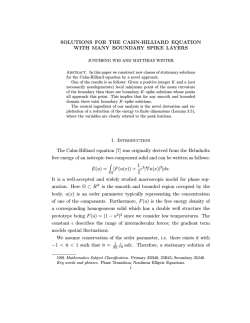
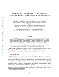


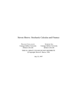
© Copyright 2026