1. Art and Diseño

Finite Differences
P. Sam Johnson
January 31, 2015
P. Sam Johnson (NITK)
Finite Differences
January 31, 2015
1 / 45
Overview
Assume that we have a table of values
(xi , yi ),
i = 0, 1, 2, . . . , n
of any function y = f (x), the values of x being equally spaced.
That is, xi = x0 + ih, i = 0, 1, 2, . . . , n. The step length h is called the
interval of differencing.
Suppose that we are required to recover the values of f (x) for some
intermediate values of x, or to obtain the derivative of f (x) for some x in
the range x0 ≤ x ≤ xn .
The methods for the solution to these problems are based on the
concept of the ‘differences’ of a function. There are three important
types of differences which we define and disucss in three lectures.
P. Sam Johnson (NITK)
Finite Differences
January 31, 2015
2 / 45
Overview
The calculus of finite differences deals with the changes that take place
in the value of the function (dependent variable), due to finite changes in
the independent variable.
Through this, we also study the relations that exist between the values
assumed by the function, whenever the independent variable changes by
(equal or unequal) finite jumps.
On the other hand, in infinitesimal calculus, we study those changes of
the function which occur when the independent variable changes
continuously in a given interval.
We shall study the variations in the function when the independent
variable changes by equal intervals.
The calculus of differences is very useful for the finding the sum of a given
series.
P. Sam Johnson (NITK)
Finite Differences
January 31, 2015
3 / 45
Differences of y
Suppose a function (usually unknown) y = f (x) is given at discrete values
of x, x0 , x1 , . . . , xn so that we have a table of values
(xi , yi ),
i = 0, 1, 2, . . . n.
The values of x being equally spaced. That is,
xi = x0 + ih,
i = 0, 1, 2, . . . , n.
If y0 , y1 , y2 , . . . , yn denote a set of values of y = f (x) on x0 , x1 , . . . , xn
respectively (note that yi = f (xi ), 0 ≤ i ≤ n), then
y1 − y0
y2 − y1
..
.
yn − yn−1
are called the differences of y .
P. Sam Johnson (NITK)
Finite Differences
January 31, 2015
4 / 45
Forward Difference Operator, ∆ (called big delta)
Denoting the differences, (y1 − y0 ), (y2 − y1 ), . . . , (yn − yn−1 ) by
∆y0 , ∆y1 , . . . , ∆yn−1
respectively, we have
∆y0 = y1 − y0 , ∆y1 = y2 − y1 , . . . , ∆yn−1 = yn − yn−1
where ∆ is called forward difference operator and ∆y0 , ∆y1 . . ., are
called first forward differences.
∆ is not a quantity but an operation.
P. Sam Johnson (NITK)
Finite Differences
January 31, 2015
5 / 45
Higher Differences
The differences of the first forward differences are called second forward
differences and are denoted by ∆2 y0 , ∆2 y1 , . . . .
The symbol ∆2 does not represent the square of a quantity but denotes
the repetition of the operation ∆.
Similarly, one can define third forward differences, fourth forward
differences, etc.
In general, the nth differences are defined as
∆n yi = ∆n−1 yi+1 − ∆n−1 yi .
The forward difference operator can be operated on function-values,
generally denoted as
∆f (x) = f (x + h) − f (x),
P. Sam Johnson (NITK)
x = x0 , x1 , . . . , xn−1 .
Finite Differences
January 31, 2015
6 / 45
Exercises
1. Evaluate ∆ tan−1 x, ∆(e x log 2x), ∆(x 2 / cos 2x).
2. Evaluate
∆
2
5x + 12
,
x 2 + 5x + 16
interval of differencing being unity.
3. Find the successive differences of f (x) = ab c x and sum the first n
differences.
4. Find the function (with suitable h) whose first difference is
(a) ax + b
(b) sin x
(c) e x
(d) e a+bx
5. Prove that the operator ∆ obeys the index law :
∆m ∆n f (x) = ∆m+n f (x)
where m and n are positive integers.
P. Sam Johnson (NITK)
Finite Differences
January 31, 2015
7 / 45
The following result can be proved by the method of induction and it helps
in expressing, any powers of ∆ operated on y (x), in terms of yi ’s. The
proof is based on continuous substitution.
Theorem
Suppose that we have a table of values (xi , yi ), i = 0, 1, 2, . . . ., n of any
function y = f (x), the values of x being equally spaced with h as the
interval of differencing. Then for any non-negative integer k,
k
X
k−i k
∆ yr =
(−1)
yr +i .
i
k
i=0
The theorem refers to the following facts:
(a) Any higher order forward difference can be expressed in terms of the
preceding differences.
(b) Any higher order forward difference can be expressed in terms of the
entries.
P. Sam Johnson (NITK)
Finite Differences
January 31, 2015
8 / 45
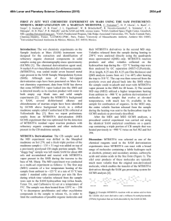
(Forward) Difference Table
Value
of
x
x0
Value
of
y = f (x)
y0
x0 + h
y1
First
Difference
∆f (x)
Second
Difference
∆2 f (x)
Third
Difference
∆3 f (x)
Fourth
Difference
∆4 f (x)
∆y0
∆2 y 0
∆3 y 0
∆y1
x0 + 2h
2
3
∆y2
x0 + 3h
y3
x0 + 4h
y4
∆4 y 0
∆ y1
y2
∆ y1
∆2 y 2
∆y3
y0 , the first entry is called the leading term. ∆y0 , ∆2 y0 , ∆3 y0 etc. are called the
leading differences. It can be seen that the differences ∆k yi with a fixed
subscript i lie along the diagonal sloping downwards and each difference is written
midway between the values substracted.
P. Sam Johnson (NITK)
Finite Differences
January 31, 2015
9 / 45
Shift Operator, E
An operator E defined as
Ef (x) = f (x + h)
is called a shift operator which results in increasing the argument by the
interval of differencing.
E n stands for the operation E being carried n times. Then
E n f (x) = f (x + nh).
The inverse operator E −1 is defined as
E −1 f (x) = f (x − h).
P. Sam Johnson (NITK)
Finite Differences
January 31, 2015
10 / 45
Relation between E and ∆
∆f (x) = f (x + h) − f (x) = Ef (x) − f (x).
Hence
Ef (x) = f (x) + ∆f (x) = (1 + ∆)f (x).
Here 1 (unity) is an operator just as E and ∆ and leaves the function
unaltered when it operates on that function. That is, 1f (x) = f (x).
Since f (x) is arbitrary, we get
E ≡ 1 + ∆.
This is known as separation of symbols. We shall define some more
operators later and establish many relations between the operators.
P. Sam Johnson (NITK)
Finite Differences
January 31, 2015
11 / 45
With the help of the operators E and ∆, we can prove the above result
which is restated below.
For any non-negative integer k,
k
X
k−i k
∆ yr =
(−1)
yr +i .
i
k
i=0
Since ∆ ≡ E − 1, by binomial expansion, the above relation can be shown.
Exercises
6. Evaluate E 0 f (x), ∆(c) and E (c) where c is a constant.
7. Say true or false : If ∆f (x) = 0, then either ∆ ≡ 0 or f (x) = 0.
8. Say true or false : E 2 f (x) and E 2 [f (x)]2 are identical.
P. Sam Johnson (NITK)
Finite Differences
January 31, 2015
12 / 45
Exercise
9. An operator T is said to be linear if
T [af (x) + bg (x)] = aT [f (x)] + bT [g (x)],
where a, b are constants. Prove that the operators E and ∆ are linear.
The following theorem says that any value of the function f (x) can be
expressed in terms of leading term and the leading differences of an
ordinary difference table. It can be proved by the method of induction.
Theorem
For all integral values of k, yk =
Pk
k
r =0 r
∆k y0 .
Exercise
10. Prove the above result with the help of the operators E and ∆.
P. Sam Johnson (NITK)
Finite Differences
January 31, 2015
13 / 45
Let f (x) be a polynomial of degree n in x. If h is the interval of the
argument, then ∆f (x) is a polynomial of degree (n − 1). Thus it is to be
noted that the result of differencing a polynomial once, reduces its degree
by one.
Theorem
Let f (x) be a polynomial of degree n in x. Then the nth difference of this
polynomial is constant. Also the (n + 1)th and higher differences are zero.
The converse of the above theorem is also true. That is, if the nth
difference of a function tabulated at equally spaced intervals are
constant, the function is a polynomial of degree n.
This fact is important in numerical analysis as it enables us to
approximate a function by a polynomial of nth degree if its nth
order differences become nearly constant.
P. Sam Johnson (NITK)
Finite Differences
January 31, 2015
14 / 45
Exercises
11. If f (x) = a0 x n + a1 x n−1 + · · · + an−1 x + an (a0 6= 0), then find
∆n f (x). Obtain ∆25 {(x − a)(x − b) · · · (x − z)} where the operand
has only 25 factors and there is no factor of the type (x − x).
12. Prove that
x
e =
∆2
E
ex .
Ee x
,
∆2 e x
the interval of differencing being unity.
13. Prove that yn − y0 is the sum of all entries in the first difference
column of the difference table for (xi , yi ), 0 ≤ i ≤ n.
That is,
n−1
X
∆yx = yn − y0 .
x=0
14. Prove that y4 = y3 + ∆y2 + ∆2 y1 + ∆3 y1 .
15. Show that y4 = y0 + 4∆y0 + 6∆2 y−1 + 10∆3 y−1 if fourth and higher
differences are zero.
P. Sam Johnson (NITK)
Finite Differences
January 31, 2015
15 / 45
Exercises
16. Prove that
n+1
n+1
n+1
y0 + y1 + · · · + yn =
y0 +
∆y0 + · · · +
∆n y0 .
1
2
n+1
17. Prove the following identity
∞
X
x=0
∞
y2x
1X
1
=
yx +
2
4
x=0
∆ ∆4
1− +
− ···
2
4
y0 .
18. Find the sum of the series,
1.2 ∆x n − 2.3 ∆2 x n + 3.4 ∆3 x n − 4.5 ∆4 x n + · · · · · ·
the interval of differencing being unity.
P. Sam Johnson (NITK)
Finite Differences
January 31, 2015
16 / 45
Backward Difference Operator, ∇ (called nabla)
The differences
y1 − y0 , y2 − y1 , . . . , yn − yn−1
are called first backward differences and they are denoted by
∇y1 , ∇y2 , · · · , ∇yn
respectively, so that
∇y1 = y1 − y0
∇y2 = y2 − y1
..
.
∇yn = yn − yn−1
where ∇ is called the backward difference operator.
P. Sam Johnson (NITK)
Finite Differences
January 31, 2015
17 / 45
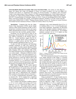
(Backward) Difference Table
Value
of
x
x0
Value
of
y = f (x)
y0
x0 + h
y1
First
Difference
∇f (x)
Second
Difference
∇2 f (x)
Third
Difference
∇3 f (x)
Fourth
Difference
∇4 f (x)
∇y1
∇2 y2
∇3 y3
∇y2
x0 + 2h
∇2 y3
y2
∇y3
x0 + 3h
∇4 y 4
∇3 y4
∇2 y4
y3
∇y4
x0 + 4h
y4
y4 , the last entry is called the last term. ∇y4 , ∇2 y4 , ∇3 y4 etc. are called
the last differences.
P. Sam Johnson (NITK)
Finite Differences
January 31, 2015
18 / 45
Central Difference Operator, δ
The central difference operator δ is defined by the relations
y1 − y0 = δy1/2 , y2 − y1 = δy3/2 , . . . , yn − yn−1 = δyn−1/2 .
Similarly, higher-order central differences are defined as
δy3/2 − δy1/2 = δ 2 y1 , δy5/2 − δy3/2 = δ 2 y2 ,
δ 2 y2 − δ 2 y1 = δ 3 y3/2
and so on.
P. Sam Johnson (NITK)
Finite Differences
January 31, 2015
19 / 45
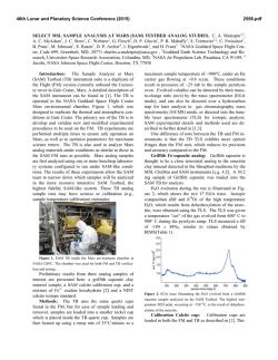
Central Difference Table
Value
of
x
x0
Value
of
y = f (x)
y0
x0 + h
y1
First
Difference
δf (x)
Second
Difference
δ 2 f (x)
Third
Difference
δ 3 f (x)
Fourth
Difference
δ 4 f (x)
δy1/2
δ 2 y1
δ 3 y3/2
δy3/2
x0 + 2h
δ 2 y2
y2
δy5/2
x0 + 3h
δ 4 y2
δ 3 y5/2
δ 2 y3
y3
δy7/2
x0 + 4h
y4
P. Sam Johnson (NITK)
Finite Differences
January 31, 2015
20 / 45
Some observations on central difference table are as
follows.
(a) The central differences on the same horizontal line have the same
suffix.
(b) The differences of odd order are known only for half values of the
suffix.
(c) The differences of even order are known only for integral values of the
suffix.
P. Sam Johnson (NITK)
Finite Differences
January 31, 2015
21 / 45
Averaging Operator, µ
It is often required to find the mean of adjacent values in the same column
of differences. We denote this mean by µ, the averaging
(mean)
1
operator µ defined by µyr = 2 yr +1/2 + yr −1/2 .
Thus µδy1 = 21 [δy1/2 + δy3/2 ], µδ 2 y3/2 = 21 [δ 2 y1 + δ 2 y2 ], . . . .
An Important Observation : We can observe the following
∆y0 = ∇y1 = δy1/2 ,
∆3 y1 = ∇3 y4 = δ 3 y5/2 .
It is only the notation which changes and not the differences.
For example, y1 − y0 = ∆y0 = ∇y1 = δy1/2 .
Of all the formulae, those involving central differences are most useful in
practice as the coefficients in such formulae decrease much more rapidly.
P. Sam Johnson (NITK)
Finite Differences
January 31, 2015
22 / 45
Exercises
Deduce the following:
20. ∆ − ∇ ≡ ∆∇ = δ 2
24. ∆ ≡ E 1/2 −E −1/2 2
25. 1 + δ 2 µ2 = 1 + δ2
21. µ ≡ (1/2)(E 1/2 + E −1/2 )
q
2
22. ∆ ≡ 21 δ 2 + δ 1 + δ4
26. µ2 ≡ 1 + (1/4)∆2
q
2+∆
27. µ ≡ 2√
≡
1+
1+∆
23. (E 1/2 + E −1/2 )(1 + ∆)1/2 ≡ 2 + ∆
28. E ∇ ≡ ∇E ≡ ∆ ≡ ∆E 1/2 .
19. ∇ ≡ 1 − E −1
P. Sam Johnson (NITK)
Finite Differences
δ2
4.
January 31, 2015
23 / 45
Exercises
29. If y = a(3)x + b(−2)x and h = 1, prove that (∆2 + ∆ − 6)y = 0.
30. Evaluate ∆10 [(1 − ax)(1 − bx 2 )(1 − cx 3 )(1 − dx 4 )].
h
i
∆f (x)
1
31. Show that ∆ f (x)
= f (x)f
(x+1) .
o
n
(x)
.
32. Prove that ∆ log f (x) = log 1 + ∆f
f (x)
33. Find the missing yx values from the first differences provided.
yx
0 - - - ∆yx 0 1 2 4 7 11
P. Sam Johnson (NITK)
Finite Differences
January 31, 2015
24 / 45
Differential Operator, D
The differential operator D is defined by
Df (x) =
d
[f (x)].
dx
Exercises
Prove the following identities.
34. E ≡ e hD (Hint: Taylor’s series)
35. hD ≡ ∆ −
∆2
2
+
∆3
3
− ···
36. hD ≡ log(1 + ∆) ≡ − log(1 − ∇) ≡ sinh−1 (µδ)
37. ∇yn+1 ≡ h(1 + 12 ∇ +
P. Sam Johnson (NITK)
5
2
12 ∇
+ · · · )yn0 .
Finite Differences
January 31, 2015
25 / 45
Exercises
38. Using the method of separation of symbols, prove the following
identities:
(a) yx − ∆n yx−n = yx−1 + ∆yx−2 + ∆2 yx−3 + · · · + ∆n−1 yx−n .
x
x2
x3
2
(b) y1 x + y2 x 2 + y3 x 3 + · · · = 1−x
y1 + (1−x)
2 ∆y1 + (1−x)3 ∆ y1 + · · · .
39. Taking fifth order differences of yx to be constant and given
y0 , y1 , y2 , y3 , y4 , y5 prove that
1
25(c − b) + 3(a − c)
y2 1 = c +
2
2
256
where a = y0 + y5 , b = y1 + y4 , c = y2 + y5 .
40. For any positive integer n, prove the following:
x
(a) ∆r nn = n−r
,
n x
(b) ∆ n = 1.
P. Sam Johnson (NITK)
r <n
Finite Differences
January 31, 2015
26 / 45
Exercises
41. Using the method of separation of symbols, prove that
2
3
y0 + y1!1 x + y2!2 x 2 + y3!3 x 3 + · · · = e x [y0 + x∆y0 + x2! ∆2 y0 + x3! ∆3 y0 + · · · ].
Hence find the sum of the following series.
3
3
3
(a) 13 + 21! x + 32! x 2 + 43! x 3 + · · · ∞
10x 2
20x 3
35x 4
56x 5
(b) 1 + 4x
1! + 2! + 3! + 4! + 5! · · · ∞.
42. Prove Montmort’s theorem that
y0 + y1 x + y2 x 2 + · · · ∞ =
y0
x∆y0
x 2 ∆2 y0
+
+
+ · · · ∞.
1−x
(1 − x)2 (1 − x)3
Hence find the sum of the series 1.2 + 2.3x + 3.4x 2 + · · · ∞.
43. Using Montmort’s theorem find the sum of the series
(a) 1.3 + 3.5x + 5.7x 2 + 7.9x 3 + · · · ∞.
(b) 12 + 22 x + 32 x 2 + 42 x 3 + · · · ∞.
44. Say true or false : ∆[f (x).g (x)] and f (x)∆g (x) are identical.
45. Prove that ∆yi zi = y1 ∆zi + zi+1 ∆yi .
P. Sam Johnson (NITK)
Finite Differences
January 31, 2015
27 / 45
Factorial Notation for Positive Integer
The continued product of factors whose first factor is x and successive
factors decrease by a constant difference h, is called a factorial function.
It is denoted by [x]n where n is a positive integer, which determines the
number of factors in [x]n . Thus
[x]n = x(x − h)(x − 2h) · · · (x − (n − 1)h).
For convention, we take [x]0 = 1.
When h = 1,
[x]n =
x!
x
= n!
(x − n)!
n
(x > n).
Exercise
46. Prove that for any positive integer n,
[x]n = (x − (n − 1)h)[x]n−1 .
P. Sam Johnson (NITK)
Finite Differences
January 31, 2015
28 / 45
First Difference and General Formula for n > 0
In fact f (x) = [x]n where n is a positive integer, is called the factorial
polynomial of degree n and the various differences of a factorial
polynomial are again factorial polynomials.
∆[x]n = nh[x]n−1 is a polynomial of degree (n − 1) in factorial notation.
In general, ∆n [x]n = n!hn , a constant term and ∆k [x]n = 0 for k > n.
When h = 1,
∆[x]n = n[x]n−1
∆2 [x]n = n(n − 1)[x]n−2
..
..
.
.
∆n [x]n = n!.
Hence differencing of functions in factorial notations resembles the
differentiating of functions when h = 1.
P. Sam Johnson (NITK)
Finite Differences
January 31, 2015
29 / 45
The factorial notation is of special utility in the theory of finite
differences. It helps in finding the successive differences of a
polynomial directly, by a simple rule of differentiation. When h = 1,
we have
∆[x]n = n[x]n−1
∆[ax + b]n = an[ax + b]n−1 .
That is, the result of differencing [x]n is analogous to that of
differentiating x n .
It is easier to find ∆[x]n than ∆r x n when a given polynomial is expressed
as factorial polynomial. Is this possible? Yes. The following theorem gives
an affirmative answer.
Theorem
Every polynomial of degree n can be expressed as a factorial polynomial of
the same degree and vice versa.
P. Sam Johnson (NITK)
Finite Differences
January 31, 2015
30 / 45
First Method : Synthetic Division
Using the method of synthetic division, we divide the given polynomial by
x, x − 1, x − 2, . . .
successively.
We put the coefficients of different powers of x in order beginning with
the highest power of x.
If any power of x is missing in order, we should first make the given
function complete by taking its coefficient as zero and then employ this
method.
P. Sam Johnson (NITK)
Finite Differences
January 31, 2015
31 / 45
Second Method : Direct Method
The method is illustrated with an example.
Suppose f (x) = x 4 − 12x 3 + 24x 2 − 30x + 9
f (x) = A[x]4 + B[x]3 + C [x]2 + D[x]1 + E
(in factorial notation) (1)
where the constants A, B, C and D are to be found.
Putting x = 0, 1, 2 and 3 in equation (1), we get four equations in A, B, C
and D. Solving them, we get the required polynomial in factorial notation.
Exercises
47. Express 2x 3 − 3x 2 + 3x − 10 in factorial notation by both the
methods.
48. Fill the blank: The coefficient of the highest power of x
(remains unchanged / may change) while
transforming a polynomial to factorial notation.
49. If f (x) = (2x + 1)(2x + 3) · · · (2x + 15), find the value of ∆4 f (x).
P. Sam Johnson (NITK)
Finite Differences
January 31, 2015
32 / 45
Reciprocal Factorial Function (Factorial Notation for
Negative Integer
We now discuss the factorial function [x]n , when n is any negative integer.
For any positive integer n, define
[x]−n =
P. Sam Johnson (NITK)
1
1
=
.
(x + h) · · · (x + nh)
[x + nh]n
Finite Differences
January 31, 2015
33 / 45
First Difference and General Formula for n < 0
The first difference of [x]−n ,
∆[x]−n = −nh[x]−(n+1) .
In general,
∆r [x]−h = (−1)r n(n + 1) · · · (n + r − 1)hr [x]−(n+r ) .
When h = 1, we have the following:
(a) ∆r [x]−n = (−1)r n(n + 1) · · · (n + r − 1)[x]−(n+r ) .
(b) ∆r [ax + b]−n = (−1)r n(n + 1) · · · (n + r − 1)ar [ax + b]−(n+r ) .
(c) ∆[x]−n = −n[x]−(n+1) .
(d) ∆[ax + b]−n = −na[ax + b]−(n+1) .
P. Sam Johnson (NITK)
Finite Differences
January 31, 2015
34 / 45
Exercises
50. Express the function
x 4 − 12x 3 + 24x 2 − 30x + 9
in factorial notation, the interval of differencing being unity.
51. Using factorial notation, obtain the function whose first difference is
x 3 + 4x 2 + 9x + 12.
52. Express 2x 3 − 3x 2 + 3x − 10 and its successive difference in factorial
notation.
53. A third degree polynomial passes through (0, 1), (1, 3), (2, 7) and
(3, 13). Find the polynomial.
54. Prove that [x]r [x − rh]n = [x]r +n .
55. Find the relation between α, β and γ in order that α + βx + γx 2 may
be expressible in one term in the factorial notation.
P. Sam Johnson (NITK)
Finite Differences
January 31, 2015
35 / 45
Inverse Operator of ∆, operated on [x]n
The process of finding yx when ∆yx is given, is known as inverse finite
difference operation. That is, if ∆yx = ux , then yx = ∆−1 ux . The
symbol ∆−1 or 1/∆ is called the inverse of the operator ∆.
We have the following important results.
[x]n+1
n+1 .
n+1
b]n = [ax+b]
a(n+1) .
(a) ∆−1 [x]n =
(b) ∆−1 [ax +
[x]−n+1
−n+1 .
−n+1
b]−n = [ax+b]
a(−n+1) .
(c) ∆−1 [x]−n =
(d) ∆−1 [ax +
P. Sam Johnson (NITK)
Finite Differences
January 31, 2015
36 / 45
Application to Summation of Series
The calculus of finite differences is very useful for finding the sum of a
given series.
The inverse operator ∆−1 is especially useful to find the sum of a series.
This is explained below.
If ur = ∆yr = yr +1 − yr , then u1 + u2 + · · · + un = yn+1 − y1 .
Exercise
Find the sum to n terms of the series.
56. 2.3.4 + 3.4.5 + 4.5.6 + · · ·
57.
58.
1
1
1
3.4.5 + 4.5.6 + 5.6.7 +
13 + 2 3 + · · · + n 3 .
P. Sam Johnson (NITK)
···
Finite Differences
January 31, 2015
37 / 45
Effect of an error on a difference table
Suppose there is an error ε in the entry y3 of a table. As higher differences are
formed, this error spreads out and is considered magnified. How it effects the
difference table, as shown below.
x
x0
y = f (x)
y0
x1 = x0 + h
y1
∆f (x)
∆2 f (x)
∆3 f (x)
∆y0
∆2 y 0
∆3 y 0 + ε
∆y1
x2 = x0 + 2h
2
y2
∆ y1 + ε
∆3 y1 − 3ε
∆y2 + ε
x3 = x0 + 3h
2
∆ y2 − 2ε
y3 + ε
∆3 y2 + 3ε
∆y3 − ε
x4 = x0 + 4h
2
y4
∆ y3 + ε
∆3 y 3 − ε
∆y4
x5 = x0 + 5h
..
.
P. Sam Johnson (NITK)
y5
..
.
2
..
.
Finite Differences
∆ y4
..
.
..
.
January 31, 2015
38 / 45
The above table shows that
(a) The error increases with the order of differences.
(b) The coefficients of ε’s in any column are the binomial coefficients of
(1 − ε)n .
Thus the errors in the fourth difference column are ε, −4ε, 6ε, −4ε, ε.
(c) The algebraic sum of the errors in any difference column is zero.
(d) The maximum error in each column, occurs opposite to the entry y3
containing the error.
The above facts enable us to detect errors in a difference table.
P. Sam Johnson (NITK)
Finite Differences
January 31, 2015
39 / 45
Exercises
59. One entry in the following table is incorrect and y is a cubic
polynomial in x. Use the difference table to locate and correct the
error.
x 0
1
2
3
4
5
6
7
y 25 21 18 18 27 45 76 123
60. The following table gives the values of y which is a polynomial of
degree five. It is known that f (3) is in error. Correct the error.
x
y
P. Sam Johnson (NITK)
0
1
1
2
2
33
3
254
4
1025
Finite Differences
5
3126
6
7777
January 31, 2015
40 / 45
To find one or more missing terms
When one or more values of y = f (x) corresponding to the equidistant
values of x are missing, we can find these using any of the following two
methods.
First Method. We assume that the missing term or terms as a, b etc. and
form the difference table. Assuming the last difference as zero, we solve
these equations for a, b. These give the missing term / terms.
Second Method. If n entries of y are given, f (x) can be represented by a
(n − 1)th degree polynomial. That is, ∆n y = 0.
Since ∆ ≡ E − 1, therefore (E − 1)n y = 0. Now expanding (E − 1)n and
substituting the given values, we obtain the missing term / terms.
P. Sam Johnson (NITK)
Finite Differences
January 31, 2015
41 / 45
Exercises
61. Find the missing term in the table:
x 2
3
4
5
6
y 45 49.2 54.1 - 67.4
62. Find the missing terms in the following data.
x 45 50 55 60 65
y 3
2
- -2.4
63. Assuming that the following values of y belong to a polynomial of
degree 4, compute the next three values.
x 0 1 2 3 4 5 6 7
y 1 -1 1 -1 1 - - -
P. Sam Johnson (NITK)
Finite Differences
January 31, 2015
42 / 45
Additional Exercises
Exercises
64. Match the following :
∆+∇
E∇
2
hD
∆−∇
∇∆
∆
µδ − log(1 − ∇)
65. Express any value of y in terms of yn and backward differences of yn .
66. Express u = x 4 − 12x 3 + 24x 2 − 30x + 9 and its successive difference
in factorial notation. Hence show that ∆5 u = 0.
67. Obtain the function whose first difference is 2x 3 − 3x 2 + 3x − 10.
68. If y =
1
(3x+1)(3x+4)(3x+7) ,
P. Sam Johnson (NITK)
evaluate ∆2 y . Also find ∆−1 y .
Finite Differences
January 31, 2015
43 / 45
Additional Exercises
Exercises
71. Prove that ∆(n Cr +1 ) =
n+1 C
r +1
−
nC
r +1 .
72. If y0 = 3, y11 = 6, y12 = 11, y13 = 18, y14 = 27, find y4 .
73. If yx is a polynomial for which fifth difference is constant and
y1 + y7 = −784, y2 + y6 = 686, y3 + y5 = 1088, find y4 .
P. Sam Johnson (NITK)
Finite Differences
January 31, 2015
44 / 45
References
Richard L. Burden and J. Douglas Faires, Numerical Analysis Theory and Applications, Cengage Learning, Singapore.
Kendall E. Atkinson, An Introduction to Numerical Analysis, Wiley
India.
David Kincaid and Ward Cheney, Numerical Analysis Mathematics of Scientific Computing, American Mathematical
Society, Providence, Rhode Island.
S.S. Sastry, Introductory Methods of Numerical Analysis, Fourth
Edition, Prentice-Hall, India.
Har Swarup Sharma, A Textbook of Numerical Analysis, Ratan
Prakashan Mandir, Delhi.
B.S. Grewal, Numerical Methods in Engineering & Science, Khanna
Publishers, Delhi.
P. Sam Johnson (NITK)
Finite Differences
January 31, 2015
45 / 45