
Generalized Low Rank Models
Generalized Low Rank Models Madeleine Udell, Corinne Horn, Reza Zadeh, and Stephen Boyd January 29, 2015 Abstract Principal components analysis (PCA) is a well-known technique for approximating a tabular data set by a low rank matrix. Here, we extend the idea of PCA to handle arbitrary data sets consisting of numerical, Boolean, categorical, ordinal, and other data types. This framework encompasses many well known techniques in data analysis, such as nonnegative matrix factorization, matrix completion, sparse and robust PCA, k-means, k-SVD, and maximum margin matrix factorization. The method handles heterogeneous data sets, and leads to coherent schemes for compressing, denoising, and imputing missing entries across all data types simultaneously. It also admits a number of interesting interpretations of the low rank factors, which allow clustering of examples or of features. We propose several parallel algorithms for fitting generalized low rank models, and describe implementations and numerical results. This manuscript is a draft. Comments sent to [email protected] are welcome. 1 Contents 1 Introduction 1.1 Previous work . . . . . . . . . . . . . . . . . . . . . . . . . . . . . . . . . . . 1.2 Organization . . . . . . . . . . . . . . . . . . . . . . . . . . . . . . . . . . . 2 PCA and quadratically regularized PCA 2.1 PCA . . . . . . . . . . . . . . . . . . . . 2.2 Quadratically regularized PCA . . . . . 2.3 Solution methods . . . . . . . . . . . . . 2.4 Missing data and matrix completion . . . 2.5 Interpretations and applications . . . . . 2.6 Offsets and scaling . . . . . . . . . . . . 4 5 7 . . . . . . 7 7 8 8 10 11 13 3 Generalized regularization 3.1 Solution methods . . . . . . . . . . . . . . . . . . . . . . . . . . . . . . . . . 3.2 Examples . . . . . . . . . . . . . . . . . . . . . . . . . . . . . . . . . . . . . 3.3 Offsets and scaling . . . . . . . . . . . . . . . . . . . . . . . . . . . . . . . . 14 14 15 19 4 Generalized loss functions 4.1 Solution methods . . . . . . . . . . . . . . . . . . . . . . . . . . . . . . . . . 4.2 Examples . . . . . . . . . . . . . . . . . . . . . . . . . . . . . . . . . . . . . 4.3 Offsets and scaling . . . . . . . . . . . . . . . . . . . . . . . . . . . . . . . . 20 20 21 23 5 Loss functions for abstract data types 5.1 Solution methods . . . . . . . . . . . . 5.2 Examples . . . . . . . . . . . . . . . . 5.3 Missing data and data imputation . . . 5.4 Interpretations and applications . . . . 5.5 Offsets and scaling . . . . . . . . . . . 5.6 Numerical examples . . . . . . . . . . . . . . . . . 24 24 25 27 28 30 30 6 Multi-dimensional loss functions 6.1 Examples . . . . . . . . . . . . . . . . . . . . . . . . . . . . . . . . . . . . . 6.2 Offsets and scaling . . . . . . . . . . . . . . . . . . . . . . . . . . . . . . . . 35 36 38 7 Algorithms 7.1 Alternating minimization 7.2 Early stopping . . . . . . 7.3 Quadratic objectives . . 7.4 Convergence . . . . . . . 7.5 Initialization . . . . . . . 38 38 39 41 42 42 . . . . . . . . . . . . . . . . . . . . . . . . . . . . . . . . . . . 2 . . . . . . . . . . . . . . . . . . . . . . . . . . . . . . . . . . . . . . . . . . . . . . . . . . . . . . . . . . . . . . . . . . . . . . . . . . . . . . . . . . . . . . . . . . . . . . . . . . . . . . . . . . . . . . . . . . . . . . . . . . . . . . . . . . . . . . . . . . . . . . . . . . . . . . . . . . . . . . . . . . . . . . . . . . . . . . . . . . . . . . . . . . . . . . . . . . . . . . . . . . . . . . . . . . . . . . . . . . . . . . . . . . . . . . . . . . . . . . . . . . . . . . . . . . . . . . . . . . . . . . . . . . . . . . . . . . . . . . . . . . . . . . . . . . . . . . . . . . . . . . . . . . . . . . . . . . . . . . . . . . . . . . . . . . . . . . . . . . . . . . . . 8 Extensions and applications 8.1 Homotopy methods . . . . . . . . . . . . . . . . . . . . . . . . . . . . . . . . 8.2 Choosing model parameters . . . . . . . . . . . . . . . . . . . . . . . . . . . 8.3 On-line optimization . . . . . . . . . . . . . . . . . . . . . . . . . . . . . . . 44 44 45 48 9 Implementations 9.1 Julia implementation . . . . . . . . . . . . . . . . . . . . . . . . . . . . . . . 9.2 Spark implementation . . . . . . . . . . . . . . . . . . . . . . . . . . . . . . 49 50 54 A Quadratically regularized PCA A.1 Solution . . . . . . . . . . . . . . . . . . . . . . . . . . . . . . . . . . . . . . A.2 Fixed points of alternating minimization . . . . . . . . . . . . . . . . . . . . 56 56 57 3 1 Introduction In applications of machine learning and data mining, one frequently encounters large collections of high dimensional data organized into a table. Each row in the table represents an example, and each column a feature or attribute. These tables may have columns of different (sometimes, non-numeric) types, and often have many missing entries. For example, in medicine, the table might record patient attributes or lab tests: each row of the table records test or survey results for a particular patient, and each column corresponds to a distinct test or survey question. The values in the table might be numerical (3.14), Boolean (yes, no), ordinal (never, sometimes, always), or categorical (A, B, O). Tests not administered or questions left blank result in missing entries in the data set. Other examples abound: in finance, the table might record known characteristics of companies or asset classes; in social science settings, it might record survey responses; in marketing, it might record known customer characteristics and purchase history. Exploratory data analysis can be difficult in this setting. To better understand a complex data set, one would like to be able to visualize archetypical examples, to cluster examples, to find correlated features, to fill in (impute) missing entries, and to remove (or identify) spurious or noisy data points. This paper introduces a templated method to enable these analyses even on large data sets with heterogeneous values and with many missing entries by embedding both the rows (examples) and columns (features) of the table into the same low dimensional vector space. If the data set consists only of numerical (real-valued) data, then a simple and wellknown technique to find this embedding is Principal Components Analysis (PCA). PCA finds a low rank matrix that minimizes the approximation error, in the least-squares sense, to the original data set. A factorization of this low rank matrix embeds the original high dimensional features into a low dimensional space. Extensions of PCA can handle missing data values, and can be used to impute missing entries. Here, we extend PCA to approximate an arbitrary data set by replacing the least-squares error used in PCA with a loss function that is appropriate for the given data type. Another extension beyond PCA is to add regularization on the low dimensional factors to impose or encourage some structure, such as sparsity or nonnegativity, in the low dimensional factors. In this paper we use the term generalized low rank model (GLRM) to refer to any low rank approximation of a data set obtained by minimizing a loss function on the approximation error together with regularization of the low dimensional factors. With these extensions of PCA, the resulting low rank representation of the data set still produces a low dimensional embedding of the data set, as in PCA. Many of the problems we must solve to find these low rank representations will be familiar. We recover an optimization formulation of nonnegative matrix factorization, matrix completion, sparse and robust PCA, k-means, k-SVD, and maximum margin matrix factorization, to name just a few. These low rank approximation problems are not convex, and in general cannot be solved globally and efficiently. There are a few exceptional problems that are known to have convex relaxations which are tight under certain conditions, and hence are efficiently (globally) 4 solvable under these conditions. However, all of these approximation problems can be heuristically (locally) solved by methods that alternate between updating the two factors in the low rank approximation. Each step involves either a convex problem, or a nonconvex problem that is simple enough that we can solve it exactly. While these alternating methods need not find the globally best low rank approximation, they are often very useful and effective for the original data analysis problem. 1.1 Previous work Unified views of matrix factorization. We are certainly not the first to note that matrix factorization algorithms may be viewed in a unified framework, parametrized by a small number of modeling decisions. The first instance we find in the literature of this unified view appeared in a paper by Collins, Dasgupta, and Schapire, [CDS01], extending PCA to use loss functions derived from any probabilistic model in the exponential family. Gordon’s Generalized2 Linear2 models [Gor02] extended the framework to loss functions derived from the generalized Bregman divergence of any convex function, which includes models such as Independent Components Analysis (ICA). Srebro’s 2004 PhD thesis [Sre04] extended the framework to other loss functions, including hinge loss and KL-divergence loss, and to other regularizers, including the nuclear norm and max-norm. Similarly, Chapter 8 in Tropp’s 2004 PhD thesis [Tro04] explored a number of new regularizers, presenting a range of clustering problems as matrix factorization problems with constraints, and anticipated the k-SVD algorithm usually attributed to Aharon, Elad, and Bruckstein [AEB06]. Singh and Gordon [SG08] offered a complete view of the state of the literature on matrix factorization in Table 1 of their 2008 paper, and noted that by changing the loss function and regularizer, one may recover algorithms including PCA, weighted PCA, k-means, k-medians, `1 SVD, probabilistic latent semantic indexing (pLSI), nonnegative matrix factorization with `2 or KL-divergence loss, exponential family PCA, and MMMF. Witten et al. introduced the statistics community to sparsity-inducing matrix factorization in a 2009 paper on penalized matrix decomposition, with applications to sparse PCA and canonical correlation analysis [WTH09]. Recently, Markovsky’s book on low rank approximation [Mar12] reviewed some of this literature, with a focus on applications in system, control, and signal processing. The GLRMs discussed in this paper include all of these models, and many more. Heterogeneous data. Many authors have proposed the use of low rank models as a tool for integrating heterogeneous data. The earliest example of this approach is canonical correlation analysis, developed by Hotelling [Hot36] in 1936 to understand the relations between two sets of variates in terms of the eigenvectors of their covariance matrix. This approach was extended by Witten et al. [WTH09] to encourage structured (e.g., sparse) factors. In the 1970s, De Leeuw et al. proposed the use of low rank models to fit data measured in nominal, ordinal and cardinal levels [DLYT76]. More recently, Goldberg et al. [GRX+ 10] used a low rank model to perform transduction (i.e., multi-label learning) in the presence of missing data by fitting a low rank model to the features and the labels 5 simultaneously. Low rank models have also been used to embed image, text and video data into a common low dimensional space [GD14], and have recently come into vogue in the natural language processing community as a means to embed words and documents into a low dimensional vector space [MCCD13, MSC+ 13, PSM14, SM14]. Algorithms. The matrix factorization literature presents a wide variety of algorithms to solve special cases of our problem. For example, there are variants on alternating least squares [DLYT76, YDLT76, TYDL77, DL84, DLM09], alternating Newton methods [Gor02, SG08], (stochastic or incremental) gradient descent [KO09, LRS+ 10, NRRW11, RRWN11, BRRT12, YYH+ 13, RR13], conjugate gradients [RS05, SJ03], expectation minimization (EM) (or “soft-impute”) methods [SJ03, MHT10, HMLZ14], multiplicative updates [LS99], and convex relaxations to semidefinite programs [SRJ04, FHB04, RFP10, FM13]. Generally, expectation minimization, which proceeds by iteratively imputing missing entries in the matrix and solving the fully observed problem, has been found to underperform relative to other methods [SG08]. However, when used in conjunction with computational tricks exploiting a particular problem structure, such as Gram matrix caching, these methods can still work extremely well [HMLZ14]. Semidefinite programming becomes computationally intractable for very large (or even just large) scale problems [RS05]; however, a theoretical analysis of optimality conditions for rank-constrainted semidefinite programs [BM03c] has led to a few algorithms for semidefinite programming based on matrix factorization [BM03b, ABEV09, JBAS10] which guarantee global optimality and converge quickly if the global solution to the problem is exactly low rank. Fast approximation algorithms for rank-constrained semidefinite programs have also been developed [SSGS11]. Gradient descent methods are often preferred for extremely large scale problems since these methods parallelize naturally in both shared memory and distributed memory architectures. See [RR13, YYH+ 13] and references therein for some recent innovative approaches to speeding up stochastic gradient descent for matrix factorization by eliminating locking and reducing interprocess communication. Contributions. The present paper differs from previous work in a number of ways. We are consistently concerned with the meaning of applying these different loss functions and regularizers to approximate a data set. The generality of our view allows us to introduce a number of loss functions and regularizers that have not previously been considered. Moreover, our perspective enables us to extend these ideas to arbitrary data sets, rather than just matrices of real numbers. A number of new considerations emerge when considering the problem so broadly. First, we must face the problem of comparing approximation errors across data of different types. For example, we must choose a scaling to trade off the loss due to a misclassification of a categorical value with an error of 0.1 (say) in predicting a real value. Second, we require algorithms that can handle the full gamut of losses and regularizers, which may be smooth or nonsmooth, finite or infinite valued, with arbitrary domain. This 6 work is the first to consider these problems in such generality, and therefore also the first to wrestle with the algorithmic consequences. Below, we give a number of algorithms appropriate for this setting, including many that have not been previously proposed in the literature. Our algorithms are all based around alternating minimization and variations on alternating minimization that are more suitable for large scale data and can take advantage of parallel computing resources. Finally, we present some new results on some old problems. For example, in Appendix A, we derive a formula for the solution to quadratically regularized PCA, and show that quadratically regularized PCA has no local nonglobal minima. 1.2 Organization The organization of this paper is as follows. We first recall some properties of PCA and its common variations to familiarize the reader with our notation. We then generalize the regularization on the low dimensional factors, and the loss function on the approximation error. Returning to the setting of heterogeneous data, we extend these dimensionality reduction techniques to abstract data-types and to multi-dimensional loss functions. Finally, we address algorithms for fitting GLRMs, discuss a few applications of GLRMs, and describe some implementations of the algorithms that we have developed. 2 PCA and quadratically regularized PCA Data matrix. In this section, we let A ∈ Rm×n be a data matrix consisting of m examples each with n numerical features. Thus Aij ∈ R is the value of the jth feature in the ith example, the ith row of A is the vector of n feature values for the ith example, and the jth column of A is the vector of the jth feature across our set of m examples. It is common to represent other data types in a numerical matrix using certain canonical encoding tricks. For example, Boolean data is often encoded as 1 (for true) and -1 (for false), ordinal data is often encoded using consecutive integers to represent the different levels of the variable, and categorical data is often encoded by creating a column for each possible value of the categorical variable, and representing the data using a 1 (true) in the column corresponding to the observed value, and -1 (false) in all other columns. We will see more systematic and principled ways to deal with these data types, and others, in §4–6. For now, we assume the entries in the data matrix consist of real numbers. 2.1 PCA PCA is one of the oldest and most widely used tools in data analysis [Pea01, Hot33]. We review some of its well-known properties here in order to set notation and as a warm-up to the variants presented later. PCA seeks a matrix Z ∈ Rm×n of rank k < min(m, n) that best approximates A in the least-squares sense. The rank constraint can be encoded implicitly by expressing Z in factored form as Z = XY , with X ∈ Rm×k , Y ∈ Rk×n . (The factorization 7 of Z is of course not unique.) The problem then reduces to choosing the matrices X and Y to minimize kA − XY k2F , where k · kF is the Frobenius norm of a matrix, i.e., the square root of the sum of the squares of the entries. We define xi ∈ R1×n to be the ith row of X, and yj ∈ Rm to be the jth column of Y , and use this notation throughout this paper. Thus xi yj = (XY )ij ∈ R denotes a dot or inner product. The PCA problem can be expressed as P Pn 2 minimize kA − XY k2F = m (1) i=1 j=1 (Aij − xi yj ) with variables X and Y . We will give several interpretations of the low rank factorization (X, Y ) solving (1) in §2.5. But for now we note that (1) can interpreted as a method for compressing the n features in the original data set to k < n new features. The row vector xi is associated with example i; we can think of it as a feature vector for the example using the compressed set of k < n features. The column vector yj is associated with the original feature j; it can be interpreted as the mapping from the original feature j into the k new features. 2.2 Quadratically regularized PCA We can add quadratic regularization on X and Y to the objective. The quadratically regularized PCA problem is Pn Pm Pm Pn 2 2 2 kx k + γ (A − x y ) + γ minimize (2) i ij i j 2 j=1 kyj k2 , i=1 j=1 i=1 with variables X ∈ Rm×k and Y ∈ Rk×n , and regularization parameter γ ≥ 0. Problem (2) can be written more concisely in matrix form as minimize kA − XY k2F + γkXk2F + γkY k2F . (3) When γ = 0, the problem reduces to the PCA problem (1). 2.3 Solution methods Singular value decomposition. It is well known that a solution to (1) can be obtained by truncating the singular value decomposition (SVD) of A [EY36]. The (compact) SVD of A is given by A = U ΣV T , where U ∈ Rm×r and V ∈ Rn×r have orthonormal columns, and Σ = diag(σ1 , . . . , σr ) ∈ Rr×r , with σ1 ≥ · · · ≥ σr > 0 and r = Rank(A). The columns of U = [u1 · · · ur ] and V = [v1 · · · vr ] are called the left and right singular vectors of A, respectively, and σ1 , . . . , σr are called the singular values of A. It is less well known that a solution to the quadratically regularized PCA problem can be obtained in the same way. (Proofs for each of the results stated in this section can be found in Appendix A.) Define U˜ = [u1 · · · uk ], ˜ = diag((σ1 − γ)+ , . . . , (σk − γ)+ ), Σ 8 V˜ = [v1 · · · vk ], (4) where (a)+ = max(a, 0). Here we have both truncated the SVD to keep only the top k singular vectors and values, and performed soft-thresholding on the singular values to reduce their values by γ. A solution to the quadratically regularized PCA problem (2) is then given by ˜ 1/2 , ˜ 1/2 V˜ T . X = U˜ Σ Y =Σ (5) For γ = 0, the solution reduces to the familiar solution to PCA (1) obtained by truncating the SVD to the top k singular values. The solution to (2) is clearly not unique: if X, Y is a solution, then so is XT , T −1 Y for any orthogonal matrix T ∈ Rk×k . When σk > σk+1 , all solutions to (2) have this form. For PCA (γ = 0), the set of solutions is significantly larger: XG, G−1 Y is a solution for any invertible matrix G ∈ Rk×k ; when σk > σk+1 , all solutions to the PCA problem have this form. The quadratically regularized PCA problem (2) (including the PCA problem as a special case) is the only problem we will encounter that can be efficiently globally solved. Alternating minimization. Here we mention an second method for solving (2), which can be scaled to large problems using parallel computing, and which can also fit the extensions of PCA that we discuss below. The alternating minimization algorithm simply alternates between minimizing the objective over the variable X, holding Y fixed, and then minimizing over Y , holding X fixed. With initial guesses for the factors X 0 and Y 0 , we repeat the iteration ! n m m X X X (Aij − xi yjl )2 + γ kxi k22 X l+1 = argmin X Y l+1 = argmin Y i=1 j=1 m X n X i=1 (Aij − xli yj )ij )2 + γ i=1 j=1 n X ! kyj k22 j=1 for l = 1, . . . until a stopping condition is satisfied. (If X and Y are full rank, or γ > 0, the minimizers above are unique; when they are not, we can take any minimizer.) This algorithm does not always work; in particular, it has stationary points that are not solutions of problem (2). But all stable stationary points of the iteration are solutions (see Appendix A), so as a practical matter, the alternating minimization method always works, i.e., the objective converges to the optimal value. The objective function is nonincreasing at each iteration, and therefore bounded. This implies, for γ > 0, that the iterates X k and Y k are bounded. Parallelizing alternating minimization. Alternating minimization parallelizes easily over examples and features. The problem of minimizing over X splits into m independent minimization problems. We can solve the simple quadratic problems Pn 2 2 minimize (6) j=1 (Aij − xi yj ) + γkxi k2 9 with variable xi , in parallel, for i = 1, . . . , m. Similarly, the problem of minimizing over Y splits into n independent quadratic problems, Pm 2 2 minimize (7) i=1 (Aij − xi yj ) + γkyj k2 with variable yj , which can be solved in parallel for j = 1, . . . , n. Caching factorizations. We can speed up the solution of the quadratic problems using a simple factorization caching technique. For ease of exposition, we assume here that X and Y have full rank k. The updates (6) and (7) can be expressed as X = AY T (Y Y T + γI)−1 , Y = (X T X + γI)−1 X T A. We show below how to efficiently compute X = AY T (Y Y T + γI)−1 ; the Y update admits a similar speedup using the same ideas. We assume here that k is modest, say, not more than a few hundred or a few thousand. (Typical values used in applications are often far smaller, on the order of tens.) The dimensions m and n, however, can be very large. First compute the Gram matrix G = Y Y T using an outer product expansion G= n X yj yjT . j=1 This sum can be computed on-line by streaming over the index j, or in parallel, split over the index j. This property allows us to scale up to extremely large problems even if we cannot store the entire matrix Y in memory. The computation of the Gram matrix requires 2k 2 n floating point operations (flops), but is trivially parallelizable: with r workers, we can expect a speedup on the order of r. We next add the diagonal matrix γI to G in k flops, and form the Cholesky factorization of G + γI in k 3 /3 flops and cache the factorization. In parallel over the rows of A, we compute D = AY T (2kn flops per row), and use the factorization of G + γI to compute D(G + γI)−1 with two triangular solves (2k 2 flops per row). These computations are also trivially parallelizable: with r workers, we can expect a speedup on the order of r. 2 ). Hence the total time required for each update with r workers scales as O( k (m+n)+kmn r T For k small compared to m and n, the time is dominated by the computation of AY . 2.4 Missing data and matrix completion Suppose we observe only entries Aij for (i, j) ∈ Ω ⊂ {1, . . . , m} × {1, . . . , n} from the matrix A, so the other entries are unknown. Then to find a low rank matrix that fits the data well, we solve the problem P 2 2 2 minimize (8) (i,j)∈Ω (Aij − xi yj ) + γkXkF + γkY kF , 10 with variables X and Y , with γ > 0. A solution of this problem gives an estimate Aˆij = xi yj for the value of those entries (i, j) 6∈ Ω that were not observed. In some applications, this data imputation (i.e., guessing entries of a matrix that are not known) is the main point. There are two very different regimes in which solving the problem (8) may be useful. Imputing missing entries to borrow strength. Consider a matrix A in which very few entries are missing. The typical approach in data analysis is to simply remove any rows with missing entries from the matrix and exclude them from subsequent analysis. If instead we solve the problem above without removing these affected rows, we “borrow strength” from the entries that are not missing to improve our global understanding of the data matrix A. In this regime we are imputing the (few) missing entries of A, using the examples that ordinarily we would discard. Low rank matrix completion. Now consider a matrix A in which most entries are missing, i.e., we only observe relatively few of the mn elements of A, so that by discarding every example with a missing feature or every feature with a missing example, we would discard the entire matrix. Then the solution to (8) becomes even more interesting: we are guessing all the entries of a (presumed low rank) matrix, given just a few of them. It is a surprising recent theoretical result that this is possible: if the original matrix A has rank k n, and least |Ω| = O(nk log n) entries are observed, then the solution to (8) exactly recovers the matrix A with high probability (subject to a few technical conditions on the structure of the matrix A) [KMO10]. Low rank matrix completion problems arise in applications like predicting customer ratings or customer purchases. Here the matrix consists of the ratings or numbers of purchases that m customers give (or make) for each of n products. The vast majority of the entries in this matrix are missing, since a customer will rate (or purchase) only a small fraction of the total number of products available. In this application, imputing a missing entry of the matrix as xi yj , for (i, j) 6∈ Ω, is guessing what rating a customer would give a product, if she were to rate it. This can used as the basis for a recommendation system, or a marketing plan. Alternating minimization. When Ω 6= {1, . . . , m} × {1, . . . , n}, the problem (8) has no known analytical solution, but it is still easy to find a local minimum using alternating minimization. Alternating minimization has been shown to converge geometrically to the global solution when the initial values of X and Y are chosen carefully [JNS13], but in general the method should be considered a heuristic. 2.5 Interpretations and applications The recovered matrices X and Y in the quadratically regularized PCA problems (2) and (8) admit a number of interesting interpretations. We introduce some of these interpreta- 11 tions now; the terminology we use here will recur throughout the paper. Of course these interpretations are related to each other, and not distinct. Feature compression. Quadratically regularized PCA (2) can be interpreted as a method for compressing the n features in the original data set to k < n new features. The row vector xi is associated with example i; we can think of it as a feature vector for the example using the compressed set of k < n features. The column vector yj is associated with the original feature j; it can be interpreted as the mapping from the original feature j into the k new features. Low-dimensional geometric embedding. We can think of each yj as associating feature j with a point in a low (k-) dimensional space. Similarly, each xi associates example i with a point in the low dimensional space. We can use these low dimensional vectors to judge which features (or examples) are similar; for example we can run a clustering algorithm on the low dimensional vectors yj (or xi ) to find groups of similar features (or examples). Archetypes. We can think of each row of Y as an archetype which captures the behavior of one of k idealized and maximally informative examples. These archetypes might also be called profiles, factors, or atoms. Every example i = 1, . . . , m is then represented (approximately) as a linear combination of these archetypes, with the row vector xi giving the coefficients. The coefficient xil gives the resemblance or loading of example i to the lth archetype. Archetypical representations. We call xi the representation of example i in terms of the archetypes. The rows of X give an embedding of the examples into Rk , where each coordinate axis corresponds to a different archetype. If the archetypes are simple to understand or interpret, then the representation of an example can provide better intuition about that example. The examples can be clustered according to their representations in order to determine a group of similar examples. Indeed, one might choose to apply any machine learning algorithm to the representations xi rather than to the initial data matrix: in contrast to the initial data, which may consist of high dimensional vectors with noisy or missing entries, the representations xi will be low dimensional, regularized, and complete. Feature representations. The columns of Y embed the features into Rk . Here, we think of the columns of X as archetypical features, and represent each feature j as a linear combination of the archetypical features. Just as with the examples, we might choose to apply any machine learning algorithm to the feature representations. For example, we might find clusters of similar features that represent redundant measurements. 12 Latent variables. Each row of X represents an example by a vector in Rk . The matrix Y maps these representations back into Rm . We might think of X as discovering the latent P variables that best explain the observed data. If the approximation error (i,j)∈Ω (Aij −xi yj )2 is small, then we view these latent variables as providing a good explanation or summary of the full data set. Probabilistic intepretation. We can give a probabilistic interpretation of X and Y . We ¯ and Y¯ have entries which are generated by taking independent suppose that the matrices X samples from a normal distribution with mean 0 and variance γ −1 for γ > 0. The entries in ¯ Y¯ are observed with noise ηij ∈ R, the matrix X ¯ Y¯ )ij + ηij , Aij = (X where the noise η in the (i, j)th entry is sampled independently from a standard normal distribution. We observe each entry (i, j) ∈ Ω. Then to find the maximum a posteriori ¯ Y¯ ), we solve (MAP) estimator (X, Y ) of (X, 2 ¯ 2 exp − γ kY¯ k2 Q maximize exp − γ2 kXk F F (i,j)∈Ω exp (−(Aij − xi yj ) ) , 2 which is equivalent, by taking logs, to (2). This interpretation explains the recommendation we gave above for imputing missing observations (i, j) 6∈ Ω. We simply use the MAP estimator xi yj to estimate the missing ¯ Y¯ )ij . Similarly, we can interpret (XY )ij for (i, j) ∈ Ω as a denoised version of the entry (X observation Aij . Auto-encoder. The matrix X encodes the data; the matrix Y decodes it back into the full space. We can view PCA as providing the best linear auto-encoder for the data; among all (bi-linear) low rank encodings (X) and decodings (Y ) of the data, PCA minimizes the squared reconstruction error. Compression. We impose an information bottleneck [TPB00] on the data by using a low rank auto-encoder to fit the data. PCA finds X and Y to maximize the information transmitted through this k-dimensional information bottleneck. We can interpret the solution as a compressed representation of the data, and use it to efficiently store or transmit the information present in the original data. 2.6 Offsets and scaling For good practical performance of a generalized low rank model, it is critical to ensure that model assumptions match the data. We saw above in §2.5 that quadratically regularized PCA corresponds to a model in which features are observed with N (0, 1) errors. If instead each column j of XY is observed with N (µj , σj2 ) errors, our model is no longer unbiased, and may fit very poorly, particularly if some of the column means µj are large. 13 For this reason it is standard practice to standardize the data before appplying PCA or quadratically regularized PCA: the column means are subtracted from each column, and the columns are normalized by their variances. (This can be done approximately; there is no need to get the scaling and offset exactly right.) Formally, define nj = |{i : (i, j) ∈ Ω}|, and let X 1 1 X Aij , σj2 = (Aij − µj )2 µj = nj nj − 1 (i,j)∈Ω (i,j)∈Ω estimate the mean and variance of each column of the data matrix. PCA or quadratically regularized PCA is then applied to the matrix whose (i, j) entry is (Aij − µj )/σj . 3 Generalized regularization It is easy to see how to extend PCA to allow arbitrary regularization on the rows of X and columns of Y . We form the regularized PCA problem Pn Pm P 2 ˜j (yj ), r (x ) + (A − x y ) + minimize (9) i i ij i j j=1 r i=1 (i,j)∈Ω with variables xi and yj , with given regularizers ri : Rk → R ∪ {∞} and r˜j : Rk → R ∪ {∞} for i = 1, . . . , n and j = 1, . . . , m. Regularized PCA (9) reduces to quadratically regularized PCA (2) when ri = γk · k22 , r˜j = γk · k22 . We do not restrict the regularizers to be convex. The objective in problem (9) can be expressed compactly in matrix notation as kA − XY k2F + r(X) + r˜(Y ), P P where r(X) = ni=1 r(xi ) and r˜(Y ) = nj=1 r˜(yj ). The regularization functions r and r˜ are separable across the rows of X, and the columns of Y , respectively. Infinite values of ri and r˜j are used to enforce constraints on the values of X and Y . For example, the regularizer 0 x≥0 ri (x) = ∞ otherwise, the indicator function of the nonnegative orthant, imposes the constraint that xi be nonnegative. Solutions to (9) need not be unique, depending on the choice of regularizers. If X and Y are a solution, then so are XT and T −1 Y , where T is any nonsingular matrix that satisfies r(U T ) = r(U ) for all U and r˜(T −1 V ) = r(V ) for all V . By varying our choice of regularizers r and r˜, we are able to represent a wide range of known models, as well as many new ones. We will discuss a number of choices for regularizers below, but turn now to methods for solving the regularized PCA problem (9). 3.1 Solution methods In general, there is no analytical solution for (9). The problem is not convex, even when r and r˜ are convex. However, when r and r˜ are convex, the problem is bi-convex: it is convex in X when Y is fixed, and convex in Y when X is fixed. 14 Alternating minimization. There is no reason to believe that alternating minimization will always converge to the global minimum of the regularized PCA problem (9); indeed, we will see many cases below in which the problem is known to have many local minima. However, alternating minimization can still be applied in this setting, and it still parallelizes over the rows of X and columns of Y . To minimize over X, we solve, in parallel, P 2 minimize (10) j:(i,j)∈Ω (Aij − xi yj ) + ri (xi ) with variable xi , for i = 1, . . . , m. Similarly, to minimize over Y , we solve, in parallel, P 2 minimize ˜i (yj ) (11) i:(i,j)∈Ω (Aij − xi yj ) + r with variable yj , for j = 1, . . . , n. When the regularizers are convex, these problems are convex. When the regularizers are not convex, there are still many cases in which we can find analytical solutions to the nonconvex subproblems (10) and (11), as we will see below. A number of concrete algorithms, in which these subproblems are solved explicitly, are given in §7. Caching factorizations. Often, the X and Y updates (10) and (11) reduce to convex quadratic programs. For example, this is the case for nonnegative matrix factorization, sparse PCA, and quadratic mixtures (which we define and discuss below in §3.2). The same factorization caching of the Gram matrix that was described above in the case of PCA can be used here to speed up the solution of these updates. Variations on this idea are described in detail in §7.3. 3.2 Examples Here and throughout the paper, we present a set of examples chosen for pedagogical clarity, not for completeness. In all of the examples below, γ > 0 is a parameter that controls the strength of the regularization, and we drop the subscripts from r (or r˜) to lighten the notation. Of course, it is possible to mix and match these regularizers, i.e., to choose different ri for different i, and choose different r˜j for different j. Nonnegative matrix factorization. Consider the regularized PCA problem (9) with r = I+ and r˜ = I+ , where I+ is the indicator function of the nonnegative reals. (Here, and throughout the paper, we define the indicator function of a set C, to be 0 when its argument is in C and ∞ otherwise.) Then a solution to problem (9) gives the matrix best approximating A that has a nonnegative factorization (i.e., a factorization into elementwise nonnegative matrices) [LS99]. The nonnegative matrix factorization problem has a rich analytical structure [Gil11, BRRT12, DS14] and a wide range of uses in practice [LS99, SBPP06, BBL+ 07, Vir07, KP07, FBD09]; hence the literature on it is extensive, and a number of specialized algorithms and codes for it are available [LS01, Lin07, KP08a, KP08b, BDKP14, KHP14, KP11]. 15 We can also replace the nonnegativity constraint with any interval constraint; for example, r and r˜ can be 0 if all entries of X and Y , respectively, are between 0 and 1, and infinite otherwise. Sparse PCA. If very few of the coefficients of X and Y are nonzero, it can be easier to interpret the archetypes and representations. We can understand each archetype using only a small number of features, and can understand each example as a combination of only a small number of archetypes. To get a sparse version of PCA, we use a sparsifying penalty as the regularization. Many variants on this basic idea have been proposed, together with a wide variety of algorithms [dEGJL04, ZHT06, SH08, Mac09, WTH09, RTA12, VCLR13]. For example, we could enforce that no entry Aij depend on more than s columns of X or of Y by setting r to be the indicator function of a s-sparse vector, i.e., 0 card(x) ≤ s r(x) = ∞ otherwise. and defining r˜(y) similarly, where card(x) denotes the cardinality (number of nonzero entries) in the vector x. The updates (10) and (11) are not convex, but one can find approximate solutions using a pursuit algorithm (see, e.g., [CDS98, TG07]), or exact solutions (for small s) using the branch and bound method [LW66, BM03a]. As a simple example, consider s = 1. Here we insist that each xi have at most one nonzero entry, which means that each example is a multiple of one of the rows of Y . The X-update is easy to carry out, by evaluating the best quadratic fit of xi with each of the k rows of Y . This reduces to choosing the row of Y that has the smallest angle to the ith row of A. The s-sparse regularization can be relaxed to a convex, but still sparsifying, regularization using r(x) = kxk1 , r˜(y) = kyk1 [ZHT06]. In this case, the X-update reduces to solving a (small) `1 -regularized least-squares problem. Orthogonal nonnegative matrix factorization. One well known property of PCA is that the principal components obtained (i.e., the columns of X and rows of Y ) are orthogonal, i.e., X T X and Y Y T are both diagonal. We can impose the same condition on a nonnegative matrix factorization. Due to nonnegativity of the matrix, two columns of X cannot be orthogonal if they both have a nonzero in the same row. Conversely, if X has only one nonzero per row, then its columns are mutually orthogonal. So an orthogonal nonnegative matrix factorization is identical to to a nonnegativity condition in addition to the 1-sparse condition described above. Orthogonal nonnegative matrix factorization can be achieved by using the regularizer 0 card(x) = 1, x ≥ 0 r(x) = ∞ otherwise, and letting r˜(y) be the indicator of the nonnegative orthant, as in NNMF. Geometrically, we can interpret this problem as modeling the data A as a union of rays. Each row of Y , interpreted as a point in Rn , defines a ray from the origin passing through 16 that point. Orthogonal nonnegative matrix factorization models each row of X as a point along one of these rays. Some authors [DLPP06] have also considered how to obtain a bi-orthogonal nonnegative matrix factorization, in which both X and Y T have orthogonal columns. By the same argument as above, we see this is equivalent to requiring both X and Y T to have only one positive entry per row, with the other entries equal to 0. Max-norm matrix factorization. We take r = r˜ = φ with 0 kxk22 ≤ µ φ(x) = ∞ otherwise. This penalty enforces that kXk22,∞ ≤ µ, kY T k22,∞ ≤ µ, where the (2, ∞) norm of a matrix X with rows xi is defined as maxi kxi k2 . This is equivalent to requiring the max-norm (sometimes called the γ2 -norm) of Z = XY , which is defined as kZkmax = inf{kXk2,∞ kY T k2,∞ : XY = Z}, to be bounded by µ. This penalty has been proposed by [LRS+ 10] as a heuristic for low rank matrix completion, which can perform better than Frobenius norm regularization when the low rank factors are known to have bounded entries. Quadratic clustering. Consider (9) with r˜ = 0. Let r be the indicator function of a selection, i.e., 0 x = el for some l ∈ {1, . . . , k} r(x) = ∞ otherwise, where el is the l-th standard basis vector. Thus xi encodes the cluster (one of k) to which the data vector (Ai1 , . . . , Aim ) is assigned. Alternating minimization on this problem reproduces the well-known k-means algorithm. The x update (10) is not a convex problem, but is easily solved. The solution is given by assigning xi to the closest archetype a cluster centroid in the context of kP (often called n ? 2 means): xi = el? for l = argminl j=1 (Aij − Ylj ) . The y update (11) is a least squares problem with the simple solution P i:(i,j)∈Ω Aij Xil , Ylj = P i:(i,j)∈Ω Xil i.e., each row of Y is updated to be the mean of the rows of A assigned to that archetype. 17 Quadratic mixtures. We can also implement partial assignment of data vectors to clusters. Take r˜ = 0, and let r be the indicator function of the set of probability vectors, i.e., Pk 0 xl ≥ 0 l=1 xl = 1, r(x) = ∞ otherwise. Subspace clustering. PCA approximates a data set by a single low dimensional subspace. We may also be interested in approximating a data set as a union of low dimensional subspaces. This problem is known as subspace clustering (see [Vid10] and references therein). Subspace clustering may also be thought of as generalizing quadratic clustering to assign each data vector to a low dimensional subspace rather than to a single cluster centroid. To frame subspace clustering as a regularized PCA problem (9), partition the columns of X into k blocks. Then let r be the indicator function of block sparsity (i.e., r(x) = 0 if only one block of x has nonzero entries, and otherwise r(x) = ∞). It is easy to perform alternating minimization on this objective function; this method is sometimes called the k-planes algorithm [Vid10, Tse00, AM04], which alternates over assigning examples to subspaces, and fitting the subspaces to the examples. Once again, the X update (10) is not a convex problem, but can be easily solved. Each block of the columns of X defines a subspace spanned by the corresponding rows of Y . We compute the distance from example i (the ith row of A) to each subspace (by solving a least squares problem), and assign example i to the subspace that minimizes the least squares error by setting xi to be the solution to the corresponding least squares problem. Many other algorithms for this problem have also been proposed, such as the k-SVD [AEB06] and sparse subspace clustering [EV09], some with provable guarantees on the quality of the recovered solution [SC12]. Supervised learning. Sometimes we want to understand the variation that a certain set of features can explain, and the variance that remains unexplainable. To this end, one natural strategy would be to regress the labels in the dataset on the features; to subtract the predicted values from the data; and to use PCA to understand the remaining variance. This procedure gives the same answer as the solution to a single regularized PCA problem. Here we present the case in which the features we wish to use in the regression are present in the data as the first column of A. To construct the regularizers, we make sure the first column of A appears as a feature in the supervised learning problem by setting r0 (x2 , . . . , xk+1 ) x1 = Ai1 ri (x) = ∞ otherwise, where r0 = 0 can be chosen as in any regularized PCA model. The regularization on the first row of Y is the regularization used in the supervised regression, and the regularization on the other rows will be that used in regularized PCA. Thus we see that regularized PCA can naturally combine supervised and unsupervised learning into a single problem. 18 Feature selection. We can use regularized PCA to perform feature selection. Consider (9) with r(x) = kxk22 and r˜(y) = kyk2 . (Notice that we are not using kyk22 .) The regularizer r˜ encourages the matrix Y˜ to be column-sparse, so many columns are all zero. If y˜j = 0, it means that feature j was uninformative, in the sense that its values do not help much in predicting any feature in the matrix A (including feature j itself). In this case we say that feature j was not selected. For this approach to make sense, it is important that the columns of the matrix A should have mean zero. Alternatively, one can use the de-biasing regularizers r0 and r˜0 introduced in §3.3 along with the feature selection regularizer introduced here. Dictionary learning. Dictionary learning (also sometimes called sparse coding) has become a popular method to design concise representations for very high dimensional data [OF97, LBRN06, MBPS09, MPS+ 09]. These representations have been shown to perform well when used as features in subsequent (supervised) machine learning tasks [RBL+ 07]. In dictionary learning, each row of A is modeled as a linear combination of dictionary atoms, represented by rows of Y . The total size of the dictionary used is often very large (k max(m, n)), but each example is represented using a very small number of atoms. To fit the model, one solves the regularized PCA problem (9) with r(x) = kxk1 , to induce sparsity in the number of atoms used to represent any given example, and with r˜(y) = kyk22 or r˜(y) = I+ (c − kyk2 ) for some c > 0 ∈ R, in order to ensure the problem is well posed. (Note that our notation transposes the usual notation in the literature on dictionary learning.) Mix and match. It is possible to combine these regularizers to obtain a factorization with any combination of the above properties. As an example, one may require that both X and Y be simultaneously sparse and nonnegative by choosing r(x) = kxk1 + I+ (x) = 1T x + I+ (x), and similarly for r˜(y). Similarly, [KP07] show how to obtain a nonnegative matrix factorization in which one factor is sparse by using r(x) = kxk21 + I+ (x) and r˜(y) = kyk22 + I+ (y); they go on to use this factorization as a clustering technique. 3.3 Offsets and scaling In our discussion of the quadratically regularized PCA problem (2), we saw that it can often be quite important to standardize the data before applying PCA. Conversely, in regularized PCA problems such as nonnegative matrix factorization, it makes no sense to standardize the data, since subtracting column means introduces negative entries into the matrix. A flexible approach is to allow an offset in the model: we solve P Pm Pn 2 minimize ˜j (yj ), (12) (i,j)∈Ω (Aij − xi yj − µj ) + i=1 ri (xi ) + j=1 r with variables xi , yj , and µj . Here, µj takes the role of the column mean, and in fact will be equal to the column mean in the trivial case k = 0. 19 An offset may be included in the standard form regularized PCA problem (9) by augmenting the problem slightly. Suppose we are given an instance of the problem (9), i.e., we are given k, r, and r˜. We can fit an offset term µj by letting k 0 = k + 1 and modifying the regularizers. Extend the regularization r : Rk → R and r˜ : Rk → R to new regularizers r0 : Rk+1 → R and r˜0 : Rk+1 → R which enforce that the first column of X is constant and the first row of Y is not penalized. Using this scheme, the first row of the optimal Y will be equal to the optimal µ in (12). Explicitly, let r(x2 , . . . , xk+1 ) x1 = 1 0 r (x) = ∞ otherwise, and r˜0 (y) = r˜(y2 , . . . , yk+1 ). (Here, we identify r(x) = r(x1 , . . . , xk ) to explicitly show the dependence on each coordinate of the vector x, and similarly for r˜.) It is also possible to introduce row offsets in the same way. 4 Generalized loss functions We may also generalize the loss function in PCA to form a generalized low rank model, Pn Pm P ˜j (yj ), minimize (13) j=1 r i=1 ri (xi ) + (i,j)∈Ω Lij (xi yj , Aij ) + where Lij : R × R → R+ are given loss functions for i = 1, . . . , m and j = 1, . . . , n. Problem (13) reduces to PCA with generalized regularization when Lij (u, a) = (a − u)2 . However, the loss function Lij can now depend on the data Aij in a more complex way. 4.1 Solution methods As before, problem (13) is not convex, even when Lij , ri and r˜j are convex; but if all these functions are convex, then the problem is bi-convex. Alternating minimization. Alternating minimization can still be used to find a local minimum, and it is still often possible to use factorization caching to speed up the solution of the subproblems that arise in alternating minimization. We defer a discussion of how to solve these subproblems explicitly to §7. Stochastic proximal gradient method. For use with extremely large scale problems, we discuss fast variants of the basic alternating minimization algorithm in §7. For example, we present an alternating directions stochastic proximal gradient method. This algorithm accesses the functions Lij , ri , and r˜j only through a subgradient or proximal interface, allowing it to generalize trivially to nearly any loss function and regularizer. We defer a more detailed discussion of this method to §7. 20 4.2 Examples Weighted PCA. A simple modification of the PCA objective is to weight the importance of fitting each element in the matrix A. In the generalized low rank model, we let Lij (u−a) = wij (a − u)2 , where wij is a weight, and take r = r˜ = 0. Unlike PCA, the weighted PCA problem has no known analytical solution [SJ03]; in fact, it is NP-hard to find an exact solution to weighted PCA [GG11], although it is not known whether approximate solutions of moderate accuracy may always be efficiently obtained. Robust PCA. Despite its widespread use, PCA is very sensitive to outliers. Many authors have proposed a robust version of PCA obtained by replacing least-squares loss with `1 loss, which is less sensitive to large outliers [CLMW11, WGR+ 09, XCS12]. They propose to solve the problem minimize kSk1 + kZk∗ (14) subject to S + Z = A, where the nuclear norm kZk∗ (also known as the trace norm) is defined to be the sum of the singular values of Z. The authors interpret Z as a robust version of the principal components of the data matrix A, and S as the sparse, possibly large noise corrupting the observations. We can frame robust PCA as a generalized low rank model problem in the following way. If Lij (u, a) = |a − u|, and r(x) = γ2 kxk22 , r˜(y) = γ2 kyk22 , then (13) becomes minimize kA − XY k1 + γ2 kXk2F + γ2 kY k2F . We can rewrite the problem by introducing a new variable Z as minimize kA − Zk1 + γ2 kXk2F + γ2 kY k2F subject to Z = XY. (15) Now we use the fact that kZk∗ = inf (1/2)kXk2F + (1/2)kY k2F : XY = Z to partially minimize over the variables X and Y holding Z constant. This results in the rank-constrained robust PCA problem minimize kSk1 + γkZk∗ subject to S + Z = A Rank(Z) ≤ k, where we have introduced the new variable S = A − Z. Nuclear norm regularization is often used to encourage solutions of rank less than k, and has applications ranging from graph embedding to linear system identification [Osn14, LV09, MF10, FHB04, Smi12]. 21 Huber PCA. The Huber function is defined as (1/2)x2 |x| ≤ 1 huber(x) = |x| − (1/2) |x| > 1. Using Huber loss, L(u, a) = huber(u − a), in place of `1 loss also yields an estimator robust to occasionaly large outliers [Hub81]. The Huber function is less sensitive to small errors |u − a| than the `1 norm, but becomes linear in the error for large errors. This choice of loss function results in a generalized low rank model formulation that is robust both to large outliers and to small Gaussian perturbations in the data. Previously, the problem of Gaussian noise in robust PCA has been treated by decomposing the matrix A = L + S + N into a low rank matrix L, a sparse matrix S, and a matrix with small Gaussian entries N by minimizing the loss kLk∗ + kSk1 + (1/2)kN k2F over all decompositions A = L + S + N of A [XCS12]. In fact, this formulation is equivalent to Huber PCA with quadratic regularization on the factors X and Y . The argument showing this is very similar to the one we made above for robust PCA. The only added ingredient is the observation that huber(x) = inf{|s| + (1/2)n2 : x = n + s}. Robust regularized PCA. We can design robust versions of all the regularized PCA problems above by the same transformation we used to design robust PCA. Simply replace the quadratic loss function with an `1 or Huber loss function. For example, k-mediods [KR09, PJ09] is obtained by using `1 loss in place of quadratic loss in the quadratic clustering problem. Similarly, robust subspace clustering [SEC13] can be obtained by using an `1 or Huber penalty in the subspace clustering problem. Quantile PCA. For some applications, it can be much worse to overestimate the entries of A than to underestimate them, or vice versa. One can capture this asymmetry by using the loss function L(u, a) = α(a − u)+ + (1 − α)(u − a)+ and choosing α ∈ (0, 1) appropriately. This loss function is sometimes called a scalene loss, and can be interpreted as performing quantile regression, e.g., fitting the 20th percentile [KB78, Koe05]. 22 Fractional PCA. For other applications, we may be interested in finding an approximation of the matrix A whose entries are close to the original matrix on a relative, rather than an absolute, scale. Here, we assume the entries Aij are all positive. The loss function a−u u−a L(u, a) = max , u a can capture this objective. A solution (X, Y ) to the resulting generalized low rank model with optimal value less than 0.10mn would allow one to claim that XY is a low rank matrix that is on average within 10% of the original matrix. Exponential family PCA. It is easy to formulate a version of PCA corresponding to any loss in the exponential family. Here we give some interesting loss functions generated by exponential families when all the entries Aij are positive. (See [CDS01] for a general treatment of exponential family PCA.) One popular loss function in the exponential family is the KL-divergence loss, a − a + u. L(u, a) = a log u which corresponds to a Poisson generative model [CDS01]. Another interesting loss function is the Itakura-Saito (IS) loss, a a −1+ , L(u, a) = log u u which has the property that it is scale invariant, so scaling a and u by the same factor produces the same loss. The β-divergence, L(u, a) = uβ auβ−1 aβ + − , β(β − 1) β β−1 generalizes both of these losses. With β = 2, we recover quadratic loss; in the limit as β → 1, we recover the KL-divergence loss; and in the limit as β → 0, we recover the IS loss. 4.3 Offsets and scaling In PCA, standardization rescales the data in order to compensate for unequal scaling in different features. It is possible to instead rescale the loss functions in order to compensate for unequal scaling. A savvy user may be able to select loss functions Lij that are already appropriately scaled to reflect the importance of fitting different columns. However, it is useful to have a default automatic scaling for use in other cases. The scaling proposed here generalizes the idea of standardization to a setting with heterogeneous loss functions. Given initial loss functions Lij , which we assume are nonnegative, for each feature j let µj = argmin µ X σj2 = Lij (µ, Aij ), i:(i,j)∈Ω X 1 Lij (µj , Aij ). nj − 1 i:(i,j)∈Ω 23 It is easy to see that µj generalizes the mean of column j, while σj2 generalizes the column variance. When Lij (u, a) = (u − a)2 for every i = 1, . . . , m, j = 1, . . . , n, µj is the mean and σj2 is the sample variance of the jth column of A. When Lij (u, a) = |u − a| for every i = 1, . . . , m, j = 1, . . . , n, µj is the median of the jth column of A, and σj2 is the sum of the absolute values of the deviations of the entries of the jth column from the median value. To fit a standardized GLRM, we rescale the loss functions by σj2 and solve P Pm Pn 2 minimize ˜j (yj ). (16) (i,j)∈Ω Lij (Aij , xi yj + µj )/σj + i=1 ri (xi ) + j=1 r Note that this problem can be recast in the standard form for a generalized low rank model (13). For the offset, we may use the same trick described in §3.3 to encode the offset in the regularization; and for the scaling, we simply replace the original loss function Lij by Lij /σj2 . 5 Loss functions for abstract data types We began our study of generalized low rank modeling by considering the best way to approximate a matrix by another matrix of lower rank. In this section, we apply the same procedure to approximate a data table with data that may not consist of real numbers, by choosing a loss function that respects the data type. We now consider our data A to be a database or table consisting of m examples (i.e., rows, samples) and n features (i.e., columns, attributes), with entries Aij drawn from a feature set Fj . The feature set Fj may be discrete or continuous. So far, we have only considered numerical data (Fj = R for j = 1, . . . , n), but now Fj can represent more abstract data types. For example, entries of A can take on Boolean values (Fj = {T, F }), integral values (Fj = 1, 2, 3, . . .), ordinal values (Fj = {very much, a little, not at all}), or consist of a tuple of these types (Fj = {(a, b) : a ∈ R}). We are given a loss function Lij : R × Fj → R. The loss Lij (u, a) describes the approximation error incurred when we represent a feature value a ∈ Fj by the number u ∈ R. We give a number of examples of these loss functions below. We now formulate a generalized low rank model on the database A as Pm Pn P ˜j (yj ), minimize (17) i=1 ri (xi ) + j=1 r (i,j)∈Ω Lij (xi yj , Aij ) + with variables X ∈ Rn×k and Y ∈ Rk×m , and with loss Lij as above and regularizers ri (xi ) : R1×k → R and r˜j (yj ) : Rk×1 → R (as before). When the domain of each loss function is R × R, we recover the generalized low rank model on a matrix (13). 5.1 Solution methods As before, this problem is not convex, but it is bi-convex if ri , and r˜j are convex, and Lij is convex in its first argument. The problem is also separable across samples i = 1, . . . , m and features j = 1, . . . , m. These properties makes it easy to perform alternating minimization on this objective. Once again, we defer a discussion of how to solve these subproblems explicitly to §7. 24 4 3 a = −1 log(1 + exp(au)) a=1 (1 − au)+ 3 2 1 0 2 1 0 −3 −2 −1 0 u 1 2 −3 3 Figure 1: Hinge loss. 5.2 a = −1 a=1 −2 −1 0 u 1 2 3 Figure 2: Logistic loss. Examples Boolean PCA. Suppose Aij ∈ {−1, 1}m×n , and we wish to approximate this Boolean matrix. For example, we might suppose that the entries of A are generated as noisy, 1bit observations from an underlying low rank matrix XY . Surprisingly, it is possible to accurately estimate the underlying matrix with only a few observations |Ω| from the matrix by solving problem (17) (under a few mild technical conditions) with an appropriate loss function [DPBW12]. We may take the loss to be L(u, a) = (1 − au)+ , which is the hinge loss (see Figure 1), and solve the problem (17) with or without regularization. When the regularization is sum of squares (r(x) = λkxk22 , r˜(y) = λkyk22 ), fixing X and minimizing over yj is equivalent to training a support vector machine (SVM) on a data set consisting of m examples with features xi and labels Aij . Hence alternating minimization for the problem (13) reduces to repeatedly training an SVM. This model has been previously considered under the name Maximum Margin Matrix Factorization (MMMF) [SRJ04, RS05]. Logistic PCA. Again supposing Aij ∈ {−1, 1}m×n , we can also use a logistic loss to measure the approximation quality. Let L(u, a) = log(1 + exp(−au)) (see Figure 2). With this loss, fixing X and minimizing over yj is equivalent to using logistic regression to predict the labels Aij . This model has been previously considered under the name logistic PCA [SSU03]. 25 a=1 a=2 a=3 a=4 a=5 1 2 3 4 5 1 2 3 4 5 1 2 3 4 5 1 2 3 4 5 1 2 3 4 5 Figure 3: Ordinal hinge loss. Poisson PCA. Now suppose the data Aij are nonnegative integers. We can use any loss function that might be used in a regression framework to predict integral data to construct a generalized low rank model for Poisson PCA. For example, we can take L(u, a) = exp(u) − au + a log a − a. This is the exponential family loss corresponding to Poisson data. (It differs from the KLdivergence loss from §4.2 only in that u has been replaced by exp(u), which allows u to take negative values.) Ordinal PCA. Suppose the data Aij denote the levels of some ordinal variable, encoded as {1, 2, . . . , d}. We wish to penalize the entries of the low rank matrix XY which deviate by many levels from the encoded ordinal value. A convex version of this penalty is given by the ordinal hinge loss, L(u, a) = a−1 X (1 − u + a0 )+ + d X (1 + u − a0 )+ , (18) a0 =a+1 a0 =1 which generalizes the hinge loss to ordinal data (see Figure 3). This loss function may be useful for encoding Likert-scale data indicating degrees of agreement with a question [Lik32]. For example, we might have Fj = {strongly disagree, disagree, neither agree nor disagree, agree, strongly agree}. We can encode these levels as the integers 1, . . . , 5 and use the above loss to fit a model to ordinal data. This approach assumes that every increment of error is equally bad: for example, that approximating “agree” by “strongly disagree” is just as bad as aproximating “neither agree nor disagree” by “agree”. In §6.1 we introduce a more flexible ordinal loss function that can learn a more flexible relationship between ordinal labels; for example, it could determine that the difference between “agree” and “strongly disagree” is smaller than the difference between “neither agree nor disagree” and “agree”. 26 Interval PCA. Suppose that the data Aij ∈ R2 are tuples denoting the endpoints of an interval, and we wish to find a low rank matrix whose entries lie inside these intervals. We can capture this objective using, for example, the deadzone-linear loss L(u, a) = max((a1 − u)+ , (u − a2 )+ ). 5.3 Missing data and data imputation We can use the solution (X, Y ) to a low rank model to impute values corresponding to missing data (i, j) 6∈ Ω. This process is sometimes also called inference. Above, we saw that the MAP estimator for the missing entry Aij was equal to xi yj . This is still true for many of the loss functions above, such as the Huber function or `1 loss, for which it makes sense for the data to take on any real value. However, to approximate abstract data types we must consider a more nuanced view. While we can still think of the solution (X, Y ) to the generalized low rank model (13) in Boolean PCA as approximating the Boolean matrix A, the solution is not a Boolean matrix. Instead we say that we have encoded the original Boolean matrix as a real-valued low rank matrix XY , or that we have embedded the original Boolean matrix into the space of realvalued matrices. To fill in missing entries in the original matrix A, we compute the value Aˆij that minimizes the loss for xi yj : Aˆij = argmin Lij (xi yj , a). a This implicitly constrains Aˆij to lie in the domain Fj of Lij . When Lij : R × R → R, as is the case for the losses in §4 above (including `2 , `1 , and Huber loss), then Aˆij = xi yj . But when the data is of an abstract type, the minimum argmina Lij (u, a) will not in general be equal to u. For example, when the data is Boolean, Lij : {0, 1} × R → R, we compute the Boolean matrix Aˆ implied by our low rank model by solving Aˆij = argmin(a(XY )ij − 1)+ a∈{0,1} for MMMF, or Aˆij = argmin log(1 + exp(−a(XY )ij )) a∈{0,1} for logistic PCA. These problems both have the simple solution Aˆij = sign(xi yj ). When Fj is finite, inference partitions the real numbers into regions Ra = {x ∈ R : Lij (u, x) = min Lij (u, a)} a corresponding to different values a ∈ Fj . When Lij is convex, these regions are intervals. 27 We can use the estimate Aˆij even when (i, j) ∈ Ω was observed. If the original observations have been corrupted by noise, we can view Aˆij as a denoised version of the original data. This is an unusual kind of denoising: both the noisy (Aij ) and denoised (Aˆij ) versions of the data lie in the abstract space Fj . 5.4 Interpretations and applications We have already discussed some interpretations of X and Y in the PCA setting. Now we reconsider those interpretations in the context of approximating these abstract data types. Archetypes. As before, we can think of each row of Y as an archetype which captures the behavior of an idealized example. However, the rows of Y are real numbers. To represent each archetype l = 1, . . . , k in the abstract space as Yl with (Yl )j ∈ Fj , we solve (Yl )j = argmin Lj (ylj , a). a∈Fj (Here we assume that the loss Lij = Lj is independent of the example i.) Archetypical representations. As before, we call xi the representation of example i in terms of the archetypes. The rows of X give an embedding of the examples into Rk , where each coordinate axis corresponds to a different archetype. If the archetypes are simple to understand or interpret, then the representation of an example can provide better intuition about that example. In contrast to the initial data, which may consist of arbitrarily complex data types, the representations xi will be low dimensional vectors, and can easily be used in a machine learning algorithm. Using the generalized low rank model, we have converted an abstract feature space into a vector space. Feature representations. The columns of Y embed the features into Rk . Here we think of the columns of X as archetypical features, and represent each feature j as a linear combination of the archetypical features. Just as with the examples, we might choose to apply any machine learning algorithm to the feature representations. This procedure allows us to compare non-numeric features using their representation in l R . For example, if the features F are Likert variables giving the extend to which respondents on a questionnaire agree with statements 1, . . . , n, we might be able to say that questions i and j are similar if kyi − yj k is small; or that question i is a more polarizing form of question j if yi = αyj , with α > 1. Even more interesting, it allows us to compare features of different types; we could say that the real-valued feature i is similar to Likert-valued question j if kyi − yj k is small. 28 Latent variables. Each row of X represents an example by a vector in Rk . The matrix Y maps these representations back into the original feature space (now nonlinearly) as described in the discussion on data imputation in §5.3. We might think of X as discovering the latent variables that best explain the observed data, with the added benefit that these latent P k variables lie in the vector space R . If the approximation error (i,j)∈Ω Lij (xi yj , Aij ) is small, then we view these latent variables as providing a good explanation or summary of the full data set. Probabilistic intepretation. We can give a probabilistic interpretation of X and Y , generalizing the hierarchical Bayesian model presented by Fithian and Mazumder in [FM13]. ¯ and Y¯ are generated according to a probability distribution We suppose that the matrices X ¯ and exp(−˜ with probability proportional to exp(−r(X)) r(Y¯ )), respectively. Our observations ¯ Y¯ are given by A of the entries in the matrix Z¯ = X ¯ Y¯ )ij ), Aij = ψij ((X where the random variable ψij (u) takes value a with probability proportional to exp (−Lij (u, a)) . We observe each entry (i, j) ∈ Ω. Then to find the maximum a posteriori (MAP) estimator ¯ Y¯ ), we solve (X, Y ) of (X, P maximize exp − (i,j)∈Ω Lij (xi yj , Aij ) exp(−r(X)) exp(−˜ r(Y )), which is equivalent, by taking logs, to the abstract generalized low rank model (17). This interpretation gives us a simple way to interpret our procedure for denoising our data or imputing missing observations (i, j) 6∈ Ω. We are simply computing the MAP estimator Aˆij . Auto-encoder. The matrix X encodes the data; the matrix Y decodes it back into the full space. We can view (17) as providing the best linear auto-encoder for the data; among all linear encodings (X) and decodings (Y ) of the data, the abstract generalized low rank model (17) minimizes the reconstruction error measured according to the loss functions Lij . Compression. We impose an information bottleneck by using a low rank auto-encoder to fit the data. The bottleneck is imposed by both the dimensionality reduction and the regularization, giving both soft and hard constraints on the information content allowed. The solution (X, Y ) to problem (17) maximizes the information transmitted through this k-dimensional bottleneck, measured according to the loss functions Lij . This X and Y give a compressed and real-valued representation that may be used to more efficiently store or transmit the information present in the data. 29 5.5 Offsets and scaling Just as in the previous section, better practical performance can often be achieved by allowing an offset in the model as described in §3.3, and automatic scaling of loss functions as described in §4.3. 5.6 Numerical examples In this section we give results of some small experiments illustrating the use of different loss functions adapted to abstract data types, and comparing their performance with quadratically regularized PCA. To fit these models, we use alternating minimization and solve the subproblems with subgradient descent. This approach is explained more fully in §7. Running the alternating subgradient method multiple times from different initial conditions yields different GLRMs, all with very similar (but not identical) fitting errors. Boolean PCA. For this experiment, we generate Boolean data A ∈ {−1, +1}n×m as A = sign X true Y true , where X true ∈ Rn×ktrue and Y true ∈ Rktrue ×m have independent, standard normal entries. We consider a problem instance with m = 50, n = 50, and ktrue = k = 10. We fit two GLRMs to this data to compare their performance. Boolean PCA uses hinge loss L(u, a) = max (1 − au, 0) and quadratic regularization r(u) = r˜(u) = .1kuk22 , and produces the model (X bool , Y bool ). Quadratically regularized PCA uses squared loss L(u, a) = (u − a)2 and the same quadratic regularization, and produces the model (X real , Y real ). Figure 4 shows the results of fitting Boolean PCA to this data. The first column shows the original ground-truth data A; the second shows the imputed data given the model, Aˆbool , generated by rounding the entries of X bool Y bool to the closest number in 0, 1 (as explained in §5.3); the third shows the error A− Aˆbool . Figure 4 shows the results of running quadratically regularized PCA on the same data, and shows A, Aˆreal , and A − Aˆreal . As expected, Boolean PCA performs substantially better than quadratically regularized PCA on this data set. On average over 100 draws from the ground truth data distribution, the misclassification error (percentage of misclassified entries) (X, Y ; A) = #{(i, j) | Aij = 6 sign (XY )ij } mn is much lower using hinge loss ((X bool , Y bool ; A) = 0.0016) than squared loss ((X real , Y real ; A) = 0.0051). The average RMS errors !1/2 m n 1 XX RMS(X, Y ; A) = (Aij − (XY )ij )2 mn i=1 j=1 using hinge loss (RMS(X bool , Y bool ; A) = 0.0816) and squared loss (RMS(X real , Y real ; A) = 0.159) also indicate an advantage for Boolean PCA. 30 boolean data glrm rank 10 recovery misclassified points Figure 4: Boolean PCA on Boolean data. boolean data pca rank 10 recovery misclassified points Figure 5: Quadratically regularized PCA on Boolean data. Censored PCA. In this example, we consider the performance of Boolean PCA when only a subset of positive entries in the Boolean matrix A ∈ {−1, 1}m×n have been observed, i.e., the data has been censored. For example, a retailer might know only a subset of the products each customer purchased; or a medical clinic might know only a subset of the diseases a patient has contracted, or of the drugs the patient has taken. Imputation can be used in this setting to (attempt to) distinguish true negatives Aij = −1 from unobserved positives Aij = +1, (i, j) 6∈ Ω. We generate a low rank matrix B = XY ∈ [0, 1]m×n with X ∈ Rm×k , Y ∈ Rk×n , where the entries of X and Y are drawn from a uniform distribution on [0, 1], m = n = 300 and k = 3. Our data matrix A is chosen by letting Aij = 1 with probability proportional to Bij , and −1 otherwise; the constant of proportionality is chosen so that half of the entries in A are positive. We fit a rank 5 GLRM to an observation set Ω consisting of 10% of the positive entries in the matrix, drawn uniformly at random, using hinge loss and quadratic regularization. That is, we solve P Pm Pn 2 2 minimize (i,j)∈Ω max(1 − xi yj Aij , 0) + γ i=1 kxi k2 + γ j=1 kyj k2 and vary the regularization parameter γ. We consider three error metrics to measure the performance of the fitted model (X, Y ): 31 normalized training error, 1 X max(1 − Aij xi yj , 0), |Ω| (i,j)∈Ω normalized test error, X 1 max(1 − Aij xi yj , 0), |ΩC | C (i,j)∈Ω and precision at 10 (p@10), which is computed as the fraction of the top ten predicted values {xi yj : (i, j) ∈ ΩC } not in the observation set for which Aij = 1. (Here, ΩC = {1, . . . , m} × {1, ldots, n} \ Ω.) Precision at 10 measures the usefulness of the model; if we predicted that the top 10 unseen elements (i, j) had values +1, how many would we get right? Figure 6 shows the regularization path as γ ranges from 0 to 40, averaged over 50 samples from the model. Here, we see that while the training error decreases as γ decreases, the test error reaches a minimum around γ = 5. Interestingly, the precision at 10 improves as the regularization increases; since precision at 10 is computed using only relative rather than absolute values of the model, it is insensitive to the shrinkage of the parameters introduced by the regularization. The grey line shows the probability of identifying a positive entry by guessing randomly; precision at 10, which exceeds 80% when γ & 30, is significantly higher. This performance is particularly impressive given that the observations Ω are generated by sampling rather than rounding the auxiliary matrix B. Mixed data types. In this experiment, we fit a GLRM to a data table with numerical, Boolean, and ordinal columns generated as follows. Let N1 , N2 , and N3 partition the column indices 1, . . . , n. Choose X true ∈ Rm×ktrue , Y true ∈ Rktrue ×n to have independent, standard normal entries. Assign entries of A as follows: j ∈ N1 xi y j sign (xi yj ) j ∈ N2 Aij = round(3xi yj + 1) j ∈ N3 , where the function round maps a to the nearest integer in the set {1, . . . , 7}. Thus, N1 corresponds to real-valued data; N2 corresponds to Boolean data; and N3 corresponds to ordinal data. We consider a problem instance in which m = 100, n1 = 40, n2 = 30, n3 = 30, and ktrue = k = 10. We fit a heterogeneous loss GLRM to this data with loss function Lreal (u, a) j ∈ N1 Lbool (u, a) j ∈ N2 Lij (u, a) = Lord (u, a) j ∈ N3 , where Lreal (u, a) = (u−a)2 , Lbool (u, a) = (1−au)+ , and Lord (u, a) is defined in equation (18), and with quadratic regularization r(u) = r˜(u) = .1kuk22 . We fit the GLRM to produce the 32 1 p@10 train error test error 0.9 8 0.8 6 0.6 0.5 4 0.4 probability of +1 normalized error 0.7 0.3 2 0.2 0.1 0 0 5 10 15 20 25 30 regularization parameter 35 40 0 Figure 6: Error metrics for Boolean GLRM on censored data. The grey line shows the probability of identifying a positive entry by guessing randomly. 33 mixed data types 12 9 6 3 0 −3 −6 −9 −12 glrm rank 10 recovery 12 9 6 3 0 −3 −6 −9 −12 misclassified points 1.0 0.8 0.6 0.4 0.2 0.0 −0.2 −0.4 −0.6 −0.8 −1.0 Figure 7: Heterogeneous loss GLRM on mixed data. model (X mix , Y mix ). For comparison, we also fit quadratically regularized PCA to the same data, using Lij (u, a) = (u − a)2 for all j and quadratic regularization r(u) = r˜(u) = .1kuk22 , to produce the model (X real , Y real ). Figure 7 shows the results of fitting the heterogeneous loss GLRM to the data. The first column shows the original ground-truth data A; the second shows the imputed data given the model, Aˆmix , generated by rounding the entries of X mix Y mix to the closest number in 0, 1 (as explained in §5.3); the third shows the error A − Aˆmix . Figure 8 corresponds to quadratically regularized PCA, and shows A, Aˆreal , and A − Aˆreal . To evaluate error for Boolean and ordinal data, we use the misclassification error defined above. For notational convenience, we let YNl (ANl ) denote Y (A) restricted to the columns Nl in order to pick out real-valued columns (l = 1), Boolean columns (l = 2), and ordinal columns (l = 3). Table 1 compare the average error (difference between imputed entries and ground truth) over 100 draws from the ground truth distribution for models using heterogeneous loss (X mix , Y mix ) and quadratically regularized loss (X real , Y real ). Columns are labeled by error metric. We use misclassification error for Boolean and ordinal data and MSE for numerical data. mix mix X ,Y X real , Y real MSE(X, YN1 ; AN1 ) 0.0224 0.0076 (X, YN2 ; AN2 ) 0.0074 0.0213 (X, YN3 ; AN3 ) 0.0531 0.0618 Table 1: Average error for numerical, Boolean, and ordinal features using GLRM with heterogenous loss and quadratically regularized loss. Missing data. Here, we explore the effect of missing entries on the accuracy of the recovered model. We generate data A as detailed above, but then censor one large block of entries in the table (constituting 3.75% of numerical, 50% of Boolean, and 50% of ordinal data), removing them from the observed set Ω. 34 mixed data types 12 9 6 3 0 −3 −6 −9 −12 pca rank 10 recovery 12 9 6 3 0 −3 −6 −9 −12 misclassified points 1.0 0.8 0.6 0.4 0.2 0.0 −0.2 −0.4 −0.6 −0.8 −1.0 Figure 8: Quadratically regularized PCA on mixed data. Figure 9 shows the results of fitting the heterogeneous loss GLRM described above on the censored data. The first column shows the original ground-truth data A; the second shows the block of data that has been removed from the observation set Ω; the third shows the imputed data given the model, Aˆmix , generated by rounding the entries of X mix Y mix to the closest number in {0, 1} (as explained in §5.3); the fourth shows the error A − Aˆmix . Figure 10 corresponds to running quadratically regularized PCA on the same data, and shows A, Aˆreal , and A − Aˆreal . While quadradically regularized PCA and the heterogeneous loss GLRM performed similarly when no data was missing, the heterogeneous loss GLRM performs much better than quadradically regularized PCA when a large block of data is censored. We compare the average error (difference between imputed entries and ground truth) over 100 draws from the ground truth distribution in Table 2. As above, we use misclassification error for Boolean and ordinal data and MSE for numerical data. mix mix X ,Y X real , Y real MSE(X, YN1 ; AN1 ) 0.392 0.561 (X, YN2 ; AN2 ) 0.2968 0.4029 (X, YN3 ; AN3 ) 0.3396 0.9418 Table 2: Average error over imputed data using a GLRM with heterogenous loss and regularized quadratic loss. 6 Multi-dimensional loss functions In this section, we generalize the procedure to allow the loss functions to depend on blocks of the matrix XY , which allows us to represent abstract data types more naturally. For example, we can now represent categorical values , permutations, distributions, and rankings. 1×dj We are given a loss ×Fj → R, where dj is the embedding dimension of P function Lij : R feature j, and d = j dj is the total dimension of the embedded features. The loss Lij (u, a) 35 mixed data types 12 9 6 3 0 −3 −6 −9 −12 remove entries 12 9 6 3 0 −3 −6 −9 −12 glrm rank 10 recovery 12 9 6 3 0 −3 −6 −9 −12 error 3.0 2.4 1.8 1.2 0.6 0.0 −0.6 −1.2 −1.8 −2.4 −3.0 Figure 9: Heterogeneous loss GLRM on missing data. mixed data types 12 9 6 3 0 −3 −6 −9 −12 remove entries 12 9 6 3 0 −3 −6 −9 −12 pca rank 10 recovery 12 9 6 3 0 −3 −6 −9 −12 error Figure 10: Quadratically regularized PCA on missing data. describes the approximation error incurred when we represent a feature value a ∈ Fj by the vector u ∈ Rdj . Let xi ∈ R1×k be the ith row of X (as before), and let Yj ∈ Rk×dj be the jth block matrix of Y so the columns of Yj correspond to the columns of embedded feature j. We now formulate a multi-dimensional generalized low rank model on the database A, Pn Pm P ˜j (Yj ), minimize (19) j=1 r i=1 ri (xi ) + (i,j)∈Ω Lij (xi Yj , Aij ) + with variables X ∈ Rn×k and Y ∈ Rk×d , and with loss Lij as above and regularizers ri (xi ) : R1×k → R (as before) and r˜j (Yj ) : Rk×dj → R. Note that the first argument of Lij is a row vector with dj entries, and the first argument of rj is a matrix with dj columns. When every entry Aij is real-valued (i.e., dj = 1), then we recover the generalized low rank model (13) seen in the previous section. 6.1 Examples Categorical PCA. Suppose that a ∈ F is a categorical variable, taking on one of d values or labels. Identify the labels with the integers {1, . . . , d}. In (19), set X L(u, a) = (1 − ua )+ + (1 + ua0 )+ , a0 ∈F , a0 6=a and use the quadratic regularizer ri = γk · k22 , r˜ = γk · k22 . Fixing X and optimizing over Y is equivalent to training one SVM per label to separate that label from all the others: the jth column of Y gives the weight vector corresponding the 36 3.0 2.4 1.8 1.2 0.6 0.0 −0.6 −1.2 −1.8 −2.4 −3.0 jth SVM. Optimizing over X identifies the low-dimensional feature vectors for each example that allow these SVMs to most accurately predict the labels. The difference between categorical PCA and Boolean PCA is in how missing labels are imputed. To impute a label for entry (i, j) with feature vector xi according to the procedure described above in 5.3, we project the representation Yj onto the line spanned by xi to form u = xi Yj . Given u, the imputed label is simply argmaxl ul . This model has the interesting property that if column l0 of Yj lies in the interior of the convex hull of the columns of Yj , then ul0 will lie in the interior of the interval [minl ul , maxl ul ] [BV04]. Hence the model will never impute label l0 for any example. We need not restrict ourselves to the loss function given above. In fact, any loss function that can be used to train a classifier for categorical variables (also called a multi-class classifier) can be used to fit a categorical PCA model, so long as the loss function depends only on the inner products between the parameters of the model and the features corresponding to each example. The loss function becomes the loss function L used in (19); the optimal parameters of the model give the optimal matrix Y , while the implied features will populate the optimal matrix X. For example, it is possible to use loss functions derived from error-correcting output codes [DB95]; the Directed Acyclic Graph SVM [PCST99]; the Crammer-Singer multi-class loss [CS02]; or the multi-category SVM [LLW04]. Ordinal PCA. We saw in §5 one way to fit a GLRM to ordinal data. Here, we use a larger embedding dimension for ordinal features. The multi-dimensional embedding will be particularly useful when the best mapping of the ordinal variable onto a linear scale is not uniform; e.g., if level 1 of the ordinal variable is much more similar to level 2 than level 2 is to level 3. Using a larger embedding dimension allows us to infer the relations between the levels from the data itself. Here we again identify the labels a ∈ F with the integers {1, . . . , d}. One approach we can use for (multi-dimensional) ordinal PCA is to solve (19) with the loss function d−1 X (1 − Ia>a0 ua0 )+ , (20) L(u, a) = a0 =1 and with quadratic regularization. Fixing X and optimizing over Y is equivalent to training an SVM to separate labels a ≤ l from a > l for each l ∈ F. This approach produces a set of hyperplanes (given by the columns of Y ) separating each level l from the next. The hyperplanes need not be parallel to each other. Permutation PCA. Suppose that a is a permutation of the numbers 1, . . . , d. Define the permutation loss d−1 X L(u, a) = (1 − uai + uai+1 )+ . i=1 This loss is zero if uai > uai+1 + 1 for i = 1, . . . , d − 1, and increases linearly when these inequalities are violated. Define sort(u) to return a permutation a ˆ of the indices 1, . . . , d so 37 that uaˆi ≥ uaˆi+1 for i = 1, . . . , d−1. It is easy to check that argmina L(u, a) = sort(u). Hence using the permutation loss function in generalized PCA (19) finds a low rank approximation of a given table of permutations. Many variants on the permutation PCA problem are possible. For example, in ranking PCA, we interpret the permutation as a ranking of the choices 1, . . . , d, and penalize deviations of many levels more strongly than deviations of only one level by choosing the loss d−1 X d X L(u, a) = (1 − uai + uaj )+ . i=1 j=i+1 From here, it is easy to generalize to a setting in which the rankings are only partially observed. Suppose that we observe pairwise comparisons a ⊆ {1, . . . , d} × {1, . . . , d}, where (i, j) ∈ a means that choice i was ranked above choice j. Then a loss function penalizing devations from these observed rankings is X L(u, a) = (1 − uai + uaj )+ . (i,j)∈a Many other modifications to ranking loss functions have been proposed in the literature that interpolate between the the two first loss functions proposed above, or which prioritize correctly predicting the top ranked choices. These losses include the area under the curve loss [Ste07], ordered weighted average of pairwise classification losses [UBG09], the weighted approximate-rank pairwise loss [WBU10], the k-order statistic loss [WYW13], and the accuracy at the top loss [BCMR12]. 6.2 Offsets and scaling Just as in the previous section, better practical performance can often be achieved by allowing an offset in the model as described in §3.3, and scaling loss functions as described in §4.3. 7 Algorithms In this section, we discuss a number of algorithms that may be used to fit generalized low rank models. 7.1 Alternating minimization We showed earlier how to use alternating minimization to find an (approximate) solution to a generalized low rank model. Algorithm (1) shows how to explicitly extend alternating minimization to a generalized low rank model (13) with observations Ω. Parallelization. Alternating minimization parallelizes naturally over examples and features. In Algorithm 1, the loops over i = 1, . . . , N and over j = 1, . . . , M may both be executed in parallel. 38 Algorithm 1 given X 0 , Y 0 for k = 1, 2, . . . do for i = 1, . . . , M do P k−1 k , Aij ) + r(x) xi = argminx j:(i,j)∈Ω Lij (xyj end for for j = 1, . . . , N do P k k yj = argminy L (x y, A ) + r ˜ (y) ij ij i i:(i,j)∈Ω end for end for 7.2 Early stopping It is not very useful to spend a lot of effort optimizing over X before we have a good estimate for Y . If an iterative algorithm is used to compute the minimum over X, it may make sense to stop the optimization over X early before going on to update Y . In general, we may consider replacing the minimization over x and y above by any update rule that moves towards the minimum. This templated algorithm is presented as Algorithm 2. Empirically, we find that this approach often finds a better local minimum than performing a full optimization over each factor in every iteration, in addition to saving computational effort on each iteration. Algorithm 2 given X 0 , Y 0 for k = 1, 2, . . . do for i = 1, . . . , M do , Y k−1 , A) xki = updateL,r (xk−1 i end for for j = 1, . . . , N do (k−1)T yjk = updateL,˜r (yj , X (k)T , AT ) end for end for We describe below a number of different update rules updateL,r by writing the X update. The Y update can be implemented similarly. (In fact, it can be implemented by substituting r˜ for r, switching the roles of X and Y , and transposing all matrix arguments.) All of the approaches outlined below can still be executed in parallel over examples (for the X update) and features (for the Y update). Gradient method. For example, we might take just one gradient step on the objective. This method can be used as long as L, r, and r˜ do not take infinite values. (If any of these functions f is not differentiable, replace ∇f below by any subgradient of f [BXM03].) 39 We implement updateL,r as follows. Let X g= ∇Lij (xi yj , Aij )yj + ∇r(xi ). j:(i,j)∈Ω Then set − αk g, xki = xk−1 i for some step size αk . For example, a common step size rule is αk = 1/k, which guarantees convergence to the globally optimal X if Y is fixed [BXM03]. Proximal gradient method. If a function takes on the value ∞, it need not have a subgradient at that point, which limits the stochastic gradient update to cases where the regularizer and loss are (finite) real-valued. When either the loss of regularizer take on infinite values, we can use a proximal gradient method. The proximal operator of a function f [PB13] is 1 proxf (z) = argmin(f (x) + kx − zk22 ). 2 x If f is the indicator function of a set C, the proximal operator of f is just (Euclidean) projection onto C. A proximal gradient update updateL,r is implemented as follows. Let X g= ∇Lij (xi yj , Aij )yj . j:(i,j)∈Ω Then set xki = proxαk r (xk−1 − αk g), i for some step size αk . The step size rule αk = 1/k guarantees convergence to the globally optimal X if Y is fixed, while using a fixed, but sufficiently small, step size α guarantees convergence to a small O(α) neighborhood around the optimum [Ber11]. Bolte et al. have shown that the iterates xki and yjk produced by the proximal gradient update rule (which they call proximal alternating linearized minimization, or PALM) globally converge to a critical point of the objective function under very mild conditions on L, r, and r˜ [BST13]. In numerical experiments, we find that using a fixed step size α on the order of 1/kgk2 gives fast convergence in practice. Stochastic gradients. Instead of computing the full gradient of L with respect to xi above, we can replace the gradient g in either the gradient or proximal gradient method by any stochastic gradient g, which is a vector that satisfies X Eg = ∇Lij (xi yj , Aij )yj . j:(i,j)∈Ω A stochastic gradient can be computed by sampling j uniformly at random from among observed features of i, and setting g = |{j : (i, j) ∈ Ω}|∇Lij (xi yj , Aij )yj . More samples from {j : (i, j) ∈ Ω} can be used to compute a less noisy stochastic gradient. 40 7.3 Quadratic objectives Here we describe an update rule for quadratic objectives and arbitrary regularizers that can be used along with the factorization caching technique described in §2.3. We assume here that the objective is given by kA − XY k2F + r(X) + r˜(Y ). We will concentrate here on the X update; as always, the Y update is exactly analogous. As in the case of quadratic regularization, we first form the Gram matrix G = Y T Y . Then the proximal gradient update is fast to evaluate: proxαk r (X − αk (GX − AY T )). But we can take advantage of the ease of inverting the Gram matrix G to design a faster algorithm. Letting f (X) = kA − XY k2F , we can use the proximal-proximal update X k+1 = proxαk r (proxαk f (X k )). This update is simply a proximal gradient step on the objective when f is replaced by the Moreau envelope of f , Mf (X) = inf0 f (X 0 ) + kX − X 0 k2F . X (See [PB13] for details.) This objective has the same minimizers as the original objective. Thus, repeating this update t times produces an update X k+1 = (proxαr (proxαf ))t (X) that approaches the alternating minimization update X k+1 = argminX (f (X) + r(X)) as t → ∞, for any constant stepsize α ≤ kGk22 . (Here, kGk2 = supkxk2 ≤1 kGxk2 is the operator norm of G.) This update can also be seen as a single iteration of ADMM when the dual variable in ADMM is initialized to 0; see [BPC+ 11]. Thus one can also use ADMM to efficiently compute the alternating minimization update for quadratic programs. For quadratic objectives with Gram matrix G = Y T Y , this update takes the simple form proxαk r ((G + 1 1 −1 I) (AY T + X)). αk αk As in §2.3, we can compute (G + α1k I)−1 (AY T + α1k X) in parallel by first caching the factorization of (G + α1k I)−1 . Hence it is advantageous to repeat this update many times before updating Y , since most of the computational effort is in forming G and AY T . For example, in the case of nonnegative least squares, this update is just Π+ ((G + 1 −1 1 I) (AY T + X)), αk αk where Π+ projects its argument onto the nonnegative orthant. 41 7.4 Convergence Alternating minimization need not converge to the same solution (or the same objective values) when initialized at different starting points. Through examples, we explore this idea here, fitting two GLRMs using the serial Julia implementation (presented in §9) of the alternating proximal gradient updates method. Global convergence for quadratically regularized PCA. Figure 11 shows the convergence of the alternating proximal gradient update method on a quadratically regularized PCA problem with randomly generated, fully observed data A = X true Y true , where entries of X true and Y true are drawn from a standard normal distribution. We pick five different random initializations of X and Y with standard normal entries to generate five different convergence trajectories. Quadratically regularized PCA is a simple problem with an analytical solution (see §2), and with no local minima (see Appendix A). Hence it should come as no surprise that the trajectories all converge to the same, globally optimal value. Local convergence for nonnegative matrix factorization. Figure 12 shows convergence of the same algorithm on a nonnegative matrix factorization model, with data generated in the same way as in Figure 11. (Note that A has some negative entries, so the minimal objective value is strictly greater than zero.) Here, we plot the convergence of the objective value, rather than the suboptimality, since we cannot provably compute the global minimum of the objective function. We see that the algorithm converges to a different optimal value (and point) depending on the initialization of X and Y . Three trajectories converge to the same optimal value (though one does so much faster than the others), one to a value that is somewhat better, and one to a value that is substantially worse. 7.5 Initialization Here, we discuss two approaches to initialization that result in provably good solutions, for special cases of the generalized low rank problem. SVD. The SVD provides a provably good initialization for the quadratic matrix completion problem (8). In separate lines of research, [KMO10] and [JNS13] guarantee convergence of alternating minimization to the global optimum if the algorithm is initialized with the SVD of the data matrix (or of a slightly modified, or trimmed, matrix), so long as the number of entries in the matrix is sufficiently large, and the entries have been chosen uniformly at random. Indeed, the method even converges quickly: [JNS13] show that this approach achieves a quadratic convergence rate. k-means++. The k-means++ algorithm is an initialization scheme designed for quadratic clustering problems. It consists of choosing an initial cluster centroid at random from the points, and then choosing the remaining k − 1 centroids from the points x that have not yet 42 objective suboptimality 105 104 103 102 101 100 0 1 2 3 time (s) Figure 11: Convergence of alternating proximal gradient updates on quadratically regularized PCA for n = m = 200, k = 2. been chosen with probability proportional to D(x)2 , where D(x) is the minimum distance of x to any previously chosen centroid. While quadratic clustering is known to be NP-hard, k-means++ followed by alternating minimization gives a solution with expected approximation ratio within O(log k) of the optimal value. (Here, the expectation is over the randomization in the initialization algorithm.) In contrast, an arbitrary initialization of the cluster centers for k-means can result in a solution whose value is arbitrarily worse than the true optimum. Heuristic initalizations for other models. These ideas provide good heuristic starting points for initializing more general low rank models. If one desires a low rank model for the data, initializing with the SVD of the data (even if the data is incomplete, and the loss function is not quadratic) can sometimes help alternating minimization find a good local optimum. Conversely, if the model rewards a solution that is spread out, as is the case in quadratic clustering or subspace clustering, it may be better to initialize the algorithm by choosing elements with probability proportional to a distance measure, as in k-means++. In the 43 ·104 1.8 objective value 1.7 1.6 1.5 1.4 1.3 0 1 2 3 time (s) Figure 12: Convergence of alternating proximal gradient updates on NNMF for n = m = 200, k = 2. k-means++ procedure, one can use the loss function L(u) as the distance metric D. 8 8.1 Extensions and applications Homotopy methods Suppose that we wish to understand the entire regularization path for a GLRM; that is, we would like to know the solution (X(γ), Y (γ)) to the problem P Pm Pn minimize ˜j (yj ) (i,j)∈Ω Lij (xi yj , Aij ) + γ i=1 ri (xi ) + γ j=1 r as a function of γ. Frequently, the regularization path may be computed almost as quickly as the solution for a single value of γ. We can achieve this by initially fitting the model with a very high value for γ, which is often a very easy problem. (For example, when r and r˜ are norms, the solution is (X, Y ) = (0, 0) for sufficiently large γ.) Then we may solve problems 44 corresponding to smaller and smaller values of γ by initializing the alternating minimization algorithm from our previous solution. For example, Figure 13 shows the regularization path for quadratically regularized Huber PCA on a synthetic data set. We generate a dataset A = XY +S with X ∈ Rm×k , Y ∈ Rk×n , and S ∈ Rm×n , with m = n = 300 and k = 3. The entries of X and Y are drawn from a standard normal distribution, while the entries of the sparse noise matrix S are drawn from a uniform distribution on [0, 1] with probability 0.05, and are 0 otherwise. We fit a rank 5 GLRM to an observation set Ω consisting of 10% of the entries in the matrix, drawn uniformly at random from {1, . . . , i} × {1, . . . , j}, using Huber loss and quadratic regularization, and vary the regularization parameter. That is, we solve P Pm Pn 2 2 minimize (i,j)∈Ω huber(xi yj , Aij ) + γ i=1 kxi k2 + γ j=1 kyj k2 and vary the regularization parameter γ. The figure plots both the normalized training error, 1 X huber(xi yj , Aij ), |Ω| (i,j)∈Ω and the normalized test error, X 1 huber(xi yj , Aij ), nm − |Ω| (i,j)6∈Ω of the fitted model (X, Y ), for γ ranging from 0 to 3. Here, we see that while the training error decreases and γ decreases, the test error reaches a minimum around γ = .5. Interestingly, it takes only three times longer (about 3 seconds) to generate the entire regularization path than it does to fit the model for a single value of the regularization parameter (about 1 second). 8.2 Choosing model parameters To form a generalized low rank model, one needs to specify the loss functions Lj , regularizers r and r˜, and a rank k. While the loss function is usually easy for a domain expert to choose, the regularizers and rank are often chosen based on statistical considerations. Here, we discuss a few methods for choosing model parameters by resampling from the data. Note, however, that there are methods not based on resampling for choosing model parameters: for example, it is possible to adapt the idea of dropout training [SHK+ 14] to regularize low-rank matrix estimation [JW14]. We can distinguish between three sources of noise or variability in the data, which give rise to three different resampling procedures. • The rows or columns of the data are chosen at random, i.e., drawn iid from some population. In this case it makes sense to resample the rows or columns. 45 test error train error 0.35 normalized error 0.3 0.25 0.2 0.15 0.1 0 0.5 1 1.5 γ 2 2.5 3 Figure 13: Regularization path. • The rows or columns may be fixed, but the indices of the observed entries in the matrix are chosen at random. In this case, it makes sense to resample from the observed entries in the matrix. • The indices of the observed entries are fixed, but the values are observed with some measurement error. In this case, it makes sense to resample the errors in the model. Each of these leads to a different reasonable kind of resampling scheme. The first two give rise to resampling schemes based on cross validation (i.e., resampling the rows, columns, or individual entries of the matrix) which we discuss further below. The third gives rise to resampling schemes based on the bootstrap or jackknife procedures, which resample from the errors or residuals after fitting the model. A number of methods using the third kind of resampling have been proposed in order to perform inference (i.e., generate confidence intervals) for PCA; see Josse et al. [JWH14] and references therein. There are three major considerations to balance in choosing the regularization and rank of the model. In the following discussion, we suppose that the regularizers r = γr0 and r˜ = γ˜ r0 have been chosen up to a scaling γ. Compression. A low rank model (X, Y ) with rank k and no sparsity represents the data table A with only (m + n)k numbers, achieving a compression ratio of (m + n)k/(mn). If the 46 factors X or Y are sparse, then we have used fewer than (m + n)k numbers to represent the data A, achieving a higher compression ratio.PWe may want to pick parameters of the model (k and γ) in order to achieve a good error (i,j)∈Ω Lj (Aij − xi yj ) for a given compression ratio. For each possible combination of model parameters, we can fit a low rank model with those parameters, observing both the error and the compression ratio. We can then choose the best model parameters (highest compression rate) achieving the error we require, or the best model parameters (lowest error rate) achieving the compression we require. Denoising. Suppose we observe every entry in a true data matrix contaminated by noise, + ij , with ij some random variable. We may wish to choose model e.g., Aij = Atrue ij parametersPto identify the truth and remove the noise: we would like to find k and γ to minimize (i,j)∈Ω Lj (Atrue − xi yj ). Applying cross validation to this problem to choose k ij and γ is somewhat tricky, since leaving out too few entries results in overfitting to the noise, while leaving out too many results in underfitting to the signal. The optimal number of entries to leave out may depend on the aspect ratio of the data, as well as on the type of noise present in the data [Per09], and is not well understood except in the case of Gaussian noise [OP09]. We explore the problem of choosing a holdout size numerically below. Predicting missing entries. Suppose we observe some entries in the matrix and wish to predict the others. A GLRM with a higher rank will always be able to fit the (noisy) data better than one of lower rank. Similarly, a GLRM P with no regularization (γ = 0) will always produce a model with a lower empirical loss (i,j)∈Ω Lj (xi yj , Aij ). However, a model with many parameters may also overfit to the noise. We can use cross validation to identify GLRMs that neither over nor underfit. Cross validation is commonly used in regression models to choose parameters such as the regularization parameter γ, as in Figure 13. In GLRMs, cross validation can also be used to choose the rank k; indeed, using a lower rank k can be considered another form of model regularization. As an example, we generate data A = XY + S with X ∈ Rm×k , Y ∈ Rk×n , and S ∈ Rm×n , with m = n = 300 and k = 3. The entries of X and Y are drawn from a standard normal distribution, while the entries of the sparse noise matrix S are drawn from a uniform distribution on [0, 3] with probability 0.05, and are 0 otherwise. We fit a rank k GLRM with huber loss and quadratic regularization γk·k22 to an observation set Ω consisting of p% of the entries in the matrix, drawn uniformly at random from {1, . . . , n} × {1, . . . , m}, varying p, γ, and k, and compute the test error. We average our results over 5 draws from A. In Figure 14, we see that the true rank k = 3 performs best on cross-validated error for any number of observations |Ω|. (Here, we show performance for γ = 0; the plot for other values of the regularization parameter is qualitatively the same.) Interestingly, it is easiest to identify the true rank with a small number of observations; higher numbers of observations make it more difficult to overfit to the data even when allowing higher ranks. In Figure 15, we consider the interdependence of our choice of γ and k. Regularization is most important when few matrix elements have been observed; the curve for each k is nearly 47 1 obs=0.1 obs=0.3 obs=0.5 obs=0.7 obs=0.9 normalized test error 0.8 0.6 0.4 0.2 0 1 2 3 k 4 5 Figure 14: Test error as a function of k, for γ = 0. flat when more than about 10% of the entries have been observed, so we show here a plot for |Ω| = .1mn. Here, we see that the true rank k = 3 performs best on cross-validated error for any value of the regularization parameter. Ranks that are too high (k > 3) benefit from increased regularization γ, whereas higher regularization hurts the performance of models with k lower than the true rank. That is, regularizing the rank (small k) can substitute for explicit regularization of the factors (large γ). Finally, in Figure 16 we consider how the fit of the model depends on the number of observations. If we correctly guess the rank k = 3, we find that the fit is insensitive to the number of observations. If our rank is either too high or too low, the fit improves significantly with more observations. 8.3 On-line optimization Suppose that new examples or features are being added to our data set continuously, and we wish to perform on-line optimization, which means that we should have a good estimate at any time for the representations of those examples xi or features yj which we have seen. This model is equivalent to adding new rows or columns to the data table A as the algorithm continues. In this setting, alternating minimization performs quite well, and has a very natural interpretation. Given an estimate for Y , when a new example is observed in row i, 48 1 k=1 k=2 k=3 k=4 k=5 0.9 normalized test error 0.8 0.7 0.6 0.5 0.4 0.3 0.2 0.1 0 1 2 3 4 5 γ Figure 15: Test error as a function of γ when 10% of entries are observed. we may solve minimize P j:(i,j)∈Ω Lij (Aij , xyj ) + r(x) with variable x to compute a representation for row i. This computation is exactly the same as one step of alternating minimization. Here, we are finding the best feature representation for the new example in terms of the (already well understood) archetypes Y . If the number of other examples previously seen is large, the addition of a single new example should not change the optimal Y by very much; hence if (X, Y ) was previously the global minimum of (13), this estimate of the feature representation for the new example will be very close to its optimal representation (i.e., the one that minimizes problem (13)). A similar interpretation holds when new columns are added to A. 9 Implementations The authors have developed and released three open source codes for modelling and fitting generalized low rank models: a basic serial implementation written in Python, a serial and shared-memory parallel implementation written in Julia, and a distributed implementation written in Scala using the Spark framework. The Julia and Spark implementations use the alternating proximal gradient method described in §7 to fit GLRMs, while the Python 49 1 k=1 k=2 k=3 k=4 k=5 normalized test error 0.8 0.6 0.4 0.2 0 0.1 0.3 0.5 |Ω|/mn 0.7 0.9 Figure 16: Test error as a function of observations, for γ = 0. implementation uses the alternating gradient method. In this section we briefly discuss these implementations, and report some timing results. For a full description and up-to-date information about available functionality, we encourage the reader to consult the on-line documentation for each of these packages. There are also many implementations available for fitting special cases of GLRMs. For example, an implementation capable of fitting any GLRM for which the subproblems in an alternating minimization method are quadratic programs was recently developed in Spark by Debasish Das [DD14]. The Python implementation can be found, together with documentation, at https://github.com/cehorn/glrm, and will not be discussed further here. 9.1 Julia implementation LowRankModels is a code written in Julia [BKSE12] for modelling and fitting GLRMs. The implementation is available on-line at https://github.com/madeleineudell/LowRankModels.jl. 50 We discuss some aspects of the usage and features of the code here. For a full description and up-to-date information about available functionality, we encourage the reader to consult the on-line documentation. Usage. To form a GLRM using LowRankModels, the user specifies • the data A (A), which can be any array or array-like data structure (e.g., a Julia DataFrame); • the observed entries obs (Ω), a list of tuples of the indices of the observed entries in the matrix, which may be omitted if all the entries in the matrix have been observed; • the list of loss functions losses (Lj , j = 1, . . . , n), one for each column of A; • the regularizers rx (r) and ry (˜ r); and • the rank k (k). For example, the following code forms and fits a k-means model with k = 5 on the matrix A ∈ Rm×n . losses = fill(quadratic(),n) rx = unitonesparse() ry = zeroreg() glrm = GLRM(A,losses,rx,ry,k) X,Y,ch = fit!(glrm) # # # # # quadratic loss x is 1-sparse unit vector y is not regularized form GLRM fit GLRM LowRankModels uses the proximal gradient method described in §7.2 to fit GLRMs. The optimal model is returned in the factors X and Y, while ch gives the convergence history. The exclamation mark suffix follows the convention in Julia denoting that the function mutates at least one of its arguments; in this case, it caches the best fit ‘X’ and ‘Y’ as ‘glrm.X’ and ‘glrm.Y’ [CE14]. Losses and regularizers must be of type Loss and Regularizer, respectively, and may be chosen from a list of supported losses and regularizers, which include • quadratic loss quadratic, • hinge loss hinge, • `1 loss l1, • huber loss huber, • ordinal hinge loss ordinal_hinge, • quadratic regularization quadreg, • no regularization zeroreg, 51 • nonnegative constraint nonnegative, and • 1-sparse constraint onesparse. • unit 1-sparse constraint unitonesparse. Users may also implement their own losses and regularizers. Shared memory parallelism. LowRankModels takes advantage of Julia’s SharedArray data structure to implement a fitting procedure that takes advantage of shared memory parallelism. While Julia does not yet support threading, SharedArrays in Julia allow separate processes on the same computer to access the same block of memory. To fit a model using multiple processes, LowRankModels loads the data A and the initial model X and Y into shared memory, broadcasts other problem data (e.g., the losses and regularizers) to each process, and assigns to each process a partition of the rows of X and columns of Y . At every iteration, each process updates its rows of X, its columns of Y , and computes its portion of the objective function, synchronizing after each of these steps to ensure that e.g.the X update is completed before the Y update begins; then the master process checks a convergence criterion and adjusts the step length. Automatic modeling. LowRankModels is capable of adding offsets to a GLRM, and of automatically scaling the loss functions, as described in §4.3. It can also automatically detect the types of different columns of a data frame and select an appropriate loss. Using these features, LowRankModels implements a method glrm(dataframe, k) that forms a rank k model on a data frame, automatically selecting loss functions and regularization that suit the data well, and ignoring any missing (NA) element in the data frame. This GLRM can then be fit with the function fit. Example. As an example, we fit a GLRM to the Motivational States Questionnaire (MSQ) data set [RA98]. This data set measures 3896 subjects on 92 aspects of mood and personality type, as well as recording the time of day the data were collected. The data include realvalued, Boolean, and ordinal measurements, and approximately 6% of the measurements are missing (NA). The following code loads the MSQ data set and encodes it in two dimensions: using RDatasets using LowRankModels # pick a data set df = RDatasets.dataset("psych","msq") # encode it! X,Y,labels,ch = fit(glrm(df,2)) 52 Figure 17 uses the rows of Y as a coordinate system to plot some of the features of the data set. Here we see the automatic embedding separates positive from negative emotions along the y axis. This embedding is notable for being interpretable despite having been generated completely automatically; of course, better embeddings may be obtained by a more careful choice of loss functions, regularizers, scaling, and embedding dimension k. 2 AtEase Content Quiet 1 Con dent Warmhearted Energetic Delighted Aroused y 0 Scornful Guilty Intense Excited Ashamed Fearful Angry Surprised Astonished Scared -1 Afraid -2 -0.2 -0.1 0.0 0.1 0.2 x Figure 17: An automatic embedding of the MSQ [RA98] data set into two dimensions. 53 9.2 Spark implementation SparkGLRM is a code written in Scala, built on the Spark cluster programming framework [ZCF+ 10], for modelling and fitting GLRMs. The implementation is available on-line at http://git.io/glrmspark. Design. In SparkGLRM, the data matrix A is split entry-wise across many machines, just as in [HMLZ14]. The model (X, Y ) is replicated and stored in memory on every machine. Thus the total computation time required to fit the model is proportional to the number of nonzeros divided by the number of cores, with the restriction that the model should fit in memory. (The authors leave to future work an extension to models that do not fit in memory, e.g., by using a parameter server [SSZ14].) Where possible, hardware acceleration (via breeze and BLAS) is used for local linear algebraic operations. At every iteration, the current model is broadcast to all machines, so there is only one copy of the model on each machine. This particularly important in machines with many cores, because it avoids duplicating the model those machines. Each core on a machine will process a partition of the input matrix, using the local copy of the model. Usage. The user provides loss functions Lij (u, a) indexed by i = 0, . . . , m − 1 and j = 0, . . . , n − 1, so a different loss function can be defined for each column, or even for each entry. Each loss function is defined by its gradient (or a subgradient). The method signature is loss grad(i: Int, j: Int, u: Double, a: Double) whose implementation can be customized by particular i and j. As an example, the following line implements squared error loss (L(u, a) = 1/2(u − a)2 ) for all entries: u - a Similarly, the user provides functions implementing the proximal operator of the regularizers r and r˜, which take a dense vector and perform the appropriate proximal operation. Experiments. We ran experiments on several large matrices. For size comparison, a very popular matrix in the recommender systems community is the Netflix Prize Matrix, which has 17770 rows, 480189 columns, and 100480507 nonzeros. Below we report results on several larger matrices, up to 10 times larger. The matrices are generated by fixing the dimensions and number of nonzeros per row, then uniformly sampling the locations for the nonzeros, and finally filling in those locations with a uniform random number in [0, 1]. We report iteration times using an Amazon EC2 cluster with 10 slaves and one master, of instance type “c3.4xlarge”. Each machine has 16 CPU cores and 30 GB of RAM. We ran SparkGLRM to fit two GLRMs on matrices of varying sizes. Table 3 gives results for quadratically regularized PCA (i.e., quadratic loss and quadratic regularization) with k = 5. 54 To illustrate the capability to write and fit custom loss functions, we also fit a GLRM using a loss function that depends on the parity of i + j: |u − a| i + j is even Lij (u, a) = (u − a)2 i + j is odd, with r(x) = kxk1 and r˜(y) = kyk22 , setting k = 10. (This loss function was chosen merely to illustrate the generality of the implementation; usually losses will be the same for each row in the same column.) The results for this custom GLRM are given in Table 4. Matrix size # nonzeros Time per iteration (s) 106 × 106 106 7 106 × 106 109 11 107 × 107 109 227 Table 3: SparkGLRM for quadratically regularized PCA, k = 5. Matrix size # nonzeros Time per iteration (s) 106 × 106 106 9 6 6 10 × 10 109 13 107 × 107 109 294 Table 4: SparkGLRM for custom GLRM, k = 10. The table gives the time per iteration. The number of iterations required for convergence depends on the size of the ambient dimension. On the matrices with the dimensions shown in Tables 3 and 4, convergence typically requires about 100 iterations, but we note that useful GLRMs often emerge after only a few tens of iterations. Acknowledgements The authors are grateful to Lester Mackey, Ben Recht, Chris R´e, Ashok Srivastava, Haesun Park, Art Owen, Trevor Hastie, Joel Tropp, Peter Stoica, and Nicolas Gillis for a number of illuminating discussions and comments on early drafts of this paper, and to Matei Zaharia and Debasish Das for their insights into creating a successful Spark implementation. This work was developed with support from the National Science Foundation Graduate Research Fellowship program (under Grant No. DGE-1147470), the Gabilan Stanford Graduate Fellowship, the Gerald J. Lieberman Fellowship, and the DARPA X-DATA program. 55 A Quadratically regularized PCA In this appendix we describe some properties of the quadratically regularized PCA problem (2), minimize kA − XY k2F + γkXk2F + γkY k2F . (21) In the sequel, we let U ΣV T = A be the SVD of A and let r be the rank of A. We assume for convenience that all the nonzero singular values σ1 > σ2 > · · · > σr > 0 of A are distinct. A.1 Solution Problem (2) is the only problem we will encounter that has an analytical solution. A solution is given by ˜ 1/2 , ˜ 1/2 V˜ T , X = U˜ Σ Y =Σ (22) ˜ = diag((σ1 − γ)+ , . . . , (σk − γ)+ ). where U˜ and V˜ are defined as in (4), and Σ To prove this, let’s consider the optimality conditions of (2). The optimality conditions are −(A − XY )Y T + γX = 0, −(A − XY )T X + γY T = 0. Multiplying the first optimality condition on the left by X T and the second on the left by Y and rearranging, we find X T (A − XY )Y T = γX T X, Y (A − XY )T X = γY Y T , which shows, by taking a transpose, that X T X = Y Y T at any stationary point. We may rewrite the optimality conditions together as −γI A X 0 XY X = AT −γI Y T (XY )T 0 YT X(Y Y T ) = Y T (X T X) X = (X T X), YT where we have used the fact that X T X = Y Y T . −γI A Now we see that (X, Y ) lies in an invariant subspace of the matrix . Recall AT −γI that V is an invariant subspace of a matrix A if AV = V M for some matrix M . If Rank(M ) ≤ Rank(A), we know that the eigenvalues of M are eigenvalues of A, and that the corresponding eigenvectors lie in the span of V . −γI A T Thus the eigenvalues of X X must be eigenvalues of , and (X, Y T ) must AT −γI −γI A span the corresponding eigenspace. More concretely, notice that is (symmetric, AT −γI T 56 and therefore) diagonalizable, with eigenvalues −γ ± σi . The larger eigenvalues −γ + σi correspond to the eigenvectors (ui , vi ), and the smaller ones −γ − σi to (ui , −vi ). −γI A T T Now, X X is positive semidefinite, so the eigenvalues shared by X X and AT −γI must be positive. Hence there is some set |Ω| ≤ k with σi ≥ γ for i ∈ Ω such that X √ has singular values −γ + σi for i ∈ Ω. (Recall that X T X = Y Y T , so Y has the same singular values as X.) Then (X, Y T ) spans the subspace generated by the vectors (ui , vi for i ∈ Ω. P We say the stationary point (X, Y ) has active subspace Ω. It is easy to verify that XY = i∈Ω ui (σi − γ)viT . Each active subspace gives rise to an orbit of stationary points. If (X, Y ) is a stationary point, then (XT, T −1 Y ) is also a stationary point so long as −(A − XY )Y T T −T + γXT = 0, −(A − XY )T XT + γY T T −T = 0, which is always true if T −T = T , i.e., T is orthogonal. This shows that the set of stationary points is invariant under orthogonal transformations. To simplify what follows, we choose a representative element for each orbit. Represent any stationary point with active subspace Ω by X = UΩ (ΣΩ − γI)1/2 , Y = (ΣΩ − γI)1/2 VΩT , where by UΩ we denote the submatrix of U with columns indexed by Ω, and similarly for P 0 Σ and V . At any value of γ, let k 0 (γ) = max{i : σi ≥ γ}. Then we have ki=0 k (γ) i (representative) stationary points, one for each choice of Ω The number of (representative) stationary points is decreasing in γ; when γ > σ1 , the only stationary point is X = 0, Y = 0. These stationary points can have quite different values. If (X, Y ) has active subspace Ω, then X X ||A − XY ||2F + γ(||X||2F + ||Y ||2F ) = σi2 + γ 2 + 2γ|σi − γ| . i∈Ω / i∈Ω From this form, it is clear that we should choose Ω to include the top singular values i = 1, . . . , k 0 (γ). Choosing any other subset Ω will result in a higher (worse) objective value: that is, the other stationary points are not global minima. A.2 Fixed points of alternating minimization Theorem 1. The quadratically regularized PCA problem (2) has only one local minimum, which is the global minimum. Our proof is similar to that of [BH89], who proved a related theorem for the case of PCA (1). P Proof. We showed above that every stationary point of (2) has the form XY = i∈Ω ui di viT , with Ω ⊆ {1, . . . , k 0 }, |Ω| ≤ k, and di = σi − γ. We use the representative element from √each √ stationary orbit described above, so each column of X is ui di and each row of Y is di viT for some i ∈ Ω. The columns of X are orthogonal, as are the rows of Y . 57 If a stationary point is not the global minimum, then σj > σi for some i ∈ Ω, j 6∈ Ω. Below, we show we can always find a descent direction if this condition holds, thus showing that the only local minimum is the global minimum. Assume we are at a stationary point with σj > σi for some i ∈ Ω, j 6∈ Ω. We will find a ˜ by replacing the column of descent direction by perturbing XY in direction uj vjT . Form X √ √ √ X containing ui di by (ui + uj ) di , and Y˜ by replacing the row of Y containing di viT by √ di (vi + vj )T . Now the regularization term increases slightly: X X ˜ 2F + kY˜ k2F ) − γ(kXk2F + kY k2F ) = (2γti0 ) + 2γdi (1 + 2 ) − 2γti0 γ(kXk = i0 ∈Ω,i0 6=i 2γdi 2 . i0 ∈Ω Meanwhile, the approximation error decreases: ˜ Y˜ k2F − kA − XY k2F = kui σi viT + uj σj vjT − (ui + uj )di (vi + vj )T k2F − (σi − di )2 − σ 2 kA − X j = kui (σi − di )viT + uj (σj − 2 di )vjT − ui di vjT − uj di viT k2F −(σi − di )2 − σj2 2 σi − di −di − (σi − di )2 − σj2 = −di σj − 2 di F = (σi − di )2 + (σj − 2 di )2 + 22 d2i − (σi − di )2 − σj2 = −2σj 2 di + 4 d2i + 22 d2i = 22 di (di − σj ) + 4 d2i , where we have used the rotational invariance of the Frobenius norm to arrive at the third ˜ Y˜ ) equality above. Hence the net change in the objective value in going from (X, Y ) to (X, is 2γdi 2 + 22 di (di − σj ) + 4 d2i = 22 di (γ + di − σj ) + 4 d2i = 22 di (σi − σj ) + 4 d2i , which is negative for small . Hence we have found a descent direction, showing that any stationary point with σj > σi for some i ∈ Ω, j 6∈ Ω is not a local minimum. 58 References [ABEV09] J. Abernethy, F. Bach, T. Evgeniou, and J.-P. Vert. A new approach to collaborative filtering: Operator estimation with spectral regularization. The Journal of Machine Learning Research, 10:803–826, 2009. [AEB06] M. Aharon, M. Elad, and A. Bruckstein. k-SVD: An algorithm for designing overcomplete dictionaries for sparse representation. IEEE Transactions on Signal Processing, 54(11):4311–4322, 2006. [AM04] P. K. Agarwal and N. H. Mustafa. k-means projective clustering. In Proceedings of the 23rd ACM SIGMOD-SIGACT-SIGART Symposium on Principles of Database Systems, pages 155–165. ACM, 2004. [BBL+ 07] M. W. Berry, M. Browne, A. N. Langville, V. P. Pauca, and R. J. Plemmons. Algorithms and applications for approximate nonnegative matrix factorization. Computational Statistics & Data Analysis, 52(1):155–173, 2007. [BCMR12] S. Boyd, C. Cortes, M. Mohri, and A. Radovanovic. Accuracy at the top. In Advances in Neural Information Processing Systems, pages 962–970, 2012. [BDKP14] R. Boyd, B. Drake, D. Kuang, and H. Park. Smallk is a C++/Python highperformance software library for nonnegative matrix factorization (NMF) and hierarchical and flat clustering using the NMF; current version 1.2.0. http: //smallk.github.io/, June 2014. [Ber11] D. P. Bertsekas. Incremental gradient, subgradient, and proximal methods for convex optimization: A survey. Optimization for Machine Learning, 2010:1–38, 2011. [BH89] P. Baldi and K. Hornik. Neural networks and principal component analysis: Learning from examples without local minima. NeuralNnetworks, 2(1):53–58, 1989. [BKSE12] J. Bezanson, S. Karpinski, V. B. Shah, and A. Edelman. Julia: A fast dynamic language for technical computing. arXiv preprint arXiv:1209.5145, 2012. [BM03a] S. Boyd and J. Mattingley. Branch and bound methods. Lecture notes for EE364b, Stanford University, 2003. [BM03b] S. Burer and R. Monteiro. A nonlinear programming algorithm for solving semidefinite programs via low-rank factorization. Mathematical Programming, 95(2):329–357, 2003. [BM03c] S. Burer and R. D. C. Monteiro. Local minima and convergence in low-rank semidefinite programming. Mathematical Programming, 103:2005, 2003. 59 [BPC+ 11] S. Boyd, N. Parikh, E. Chu, B. Peleato, and J. Eckstein. Distributed optimization and statistical learning via the alternating direction method of multipliers. Foundations and Trends in Machine Learning, 3(1):1–122, 2011. [BRRT12] V. Bittorf, B. Recht, C. R´e, and J. A. Tropp. Factoring nonnegative matrices with linear programs. Advances in Neural Information Processing Systems, 25:1223–1231, 2012. [BST13] J. Bolte, S. Sabach, and M. Teboulle. Proximal alternating linearized minimization for nonconvex and nonsmooth problems. Mathematical Programming, pages 1–36, 2013. [BV04] S. Boyd and L. Vandenberghe. Convex Optimization. Cambridge University Press, 2004. [BXM03] S. Boyd, L. Xiao, and A. Mutapcic. Subgradient methods. Lecture notes for EE364b, Stanford University, 2003. [CDS98] S. S. Chen, D. L. Donoho, and M. A. Saunders. Atomic decomposition by basis pursuit. SIAM Journal on Scientific Computing, 20(1):33–61, 1998. [CDS01] M. Collins, S. Dasgupta, and R. E. Schapire. A generalization of principal component analysis to the exponential family. In Advances in Neural Information Processing Systems, volume 13, page 23, 2001. [CE14] J. Chen and A. Edelman. Parallel prefix polymorphism permits parallelization, presentation & proof. arXiv preprint arXiv:1410.6449, 2014. [CLMW11] E. J. Cand`es, X. Li, Y. Ma, and J. Wright. Robust principal component analysis? Journal of the ACM (JACM), 58(3):11, 2011. [CS02] K. Crammer and Y. Singer. On the algorithmic implementation of multiclass kernel-based vector machines. The Journal of Machine Learning Research, 2:265– 292, 2002. [DB95] T. G. Dietterich and G. Bakiri. Solving multiclass learning problems via errorcorrecting output codes. CoRR, cs.AI/9501101, 1995. [DD14] D. Das and S. Das. Quadratic programing solver for non-negative matrix factorization with spark. In Spark Summit 2014, 2014. [dEGJL04] A. d’Aspremont, L. El Ghaoui, M. I. Jordan, and G. R. Lanckriet. A direct formulation for sparse PCA using semidefinite programming. In Advances in Neural Information Processing Systems, volume 16, pages 41–48, 2004. [DL84] J. De Leeuw. The Gifi system of nonlinear multivariate analysis. Data analysis and informatics, 3:415–424, 1984. 60 [DLM09] J. De Leeuw and P. Mair. Gifi methods for optimal scaling in R: The package homals. Journal of Statistical Software, pages 1–30, 2009. [DLPP06] C. Ding, T. Li, W. Peng, and H. Park. Orthogonal nonnegative matrix tfactorizations for clustering. In Proceedings of the 12th ACM SIGKDD International Conference on Knowledge Discovery and Data Mining, pages 126–135. ACM, 2006. [DLYT76] J. De Leeuw, F. Young, and Y. Takane. Additive structure in qualitative data: An alternating least squares method with optimal scaling features. Psychometrika, 41(4):471–503, 1976. [DPBW12] M. Davenport, Y. Plan, E. Berg, and M. Wootters. 1-bit matrix completion. arXiv preprint arXiv:1209.3672, 2012. [DS14] A. Damle and Y. Sun. Random projections for non-negative matrix factorization. arXiv preprint arXiv:1405.4275, 2014. [EV09] E. Elhamifar and R. Vidal. Sparse subspace clustering. In IEEE Conference on Computer Vision and Pattern Recognition, 2009, pages 2790–2797. IEEE, 2009. [EY36] C. Eckart and G. Young. The approximation of one matrix by another of lower rank. Psychometrika, 1(3):211–218, 1936. [FBD09] C. F´evotte, N. Bertin, and J. Durrieu. Nonnegative matrix factorization with the Itakura-Saito divergence: With application to music analysis. Neural Computation, 21(3):793–830, 2009. [FHB04] M. Fazel, H. Hindi, and S. Boyd. Rank minimization and applications in system theory. In Proceedings of the 2004 American Control Conference (ACC), volume 4, pages 3273–3278. IEEE, 2004. [FM13] W. Fithian and R. Mazumder. Scalable convex methods for flexible low-rank matrix modeling. arXiv preprint arXiv:1308.4211, 2013. [GD14] A. Gress and I. Davidson. A flexible framework for projecting heterogeneous data. In Proceedings of the 23rd ACM International Conference on Conference on Information and Knowledge Management, CIKM ’14, pages 1169–1178, New York, NY, USA, 2014. ACM. [GG11] N. Gillis and F. Glineur. Low-rank matrix approximation with weights or missing data is NP-hard. SIAM Journal on Matrix Analysis and Applications, 32(4):1149–1165, 2011. [Gil11] N. Gillis. Nonnegative matrix factorization: Complexity, algorithms and applications. PhD thesis, UCL, 2011. 61 [Gor02] G. J. Gordon. Generalized2 linear2 models. In Advances in Neural Information Processing Systems, pages 577–584, 2002. [GRX+ 10] A. Goldberg, B. Recht, J. Xu, R. Nowak, and X. Zhu. Transduction with matrix completion: Three birds with one stone. In Advances in neural information processing systems, pages 757–765, 2010. [HMLZ14] T. Hastie, R. Mazumder, J. Lee, and R. Zadeh. Matrix completion and low-rank svd via fast alternating least squares. arXiv, 2014. [Hot33] H. Hotelling. Analysis of a complex of statistical variables into principal components. Journal of Educational Psychology, 24(6):417, 1933. [Hot36] H. Hotelling. Relations between two sets of variates. Biometrika, 28(3-4):321– 377, 1936. [Hub81] P. Huber. Robust statistics. Wiley, New York, 1981. [JBAS10] M. Journ´ee, F. Bach, P. Absil, and R. Sepulchre. Low-rank optimization on the cone of positive semidefinite matrices. SIAM Journal on Optimization, 20(5):2327–2351, 2010. [JNS13] P. Jain, P. Netrapalli, and S. Sanghavi. Low-rank matrix completion using alternating minimization. In Proceedings of the 45th annual ACM Symposium on the Theory of Computing, pages 665–674. ACM, 2013. [JW14] J. Josse and S. Wager. Stable autoencoding: A flexible framework for regularized low-rank matrix estimation. arXiv preprint arXiv:1410.8275, 2014. [JWH14] J. Josse, S. Wager, and F. Husson. Confidence areas for fixed-effects pca. arXiv preprint arXiv:1407.7614, 2014. [KB78] R. Koenker and J. G. Bassett. Regression quantiles. Econometrica: Journal of the Econometric Society, pages 33–50, 1978. [KHP14] J. Kim, Y. He, and H. Park. Algorithms for nonnegative matrix and tensor factorizations: A unified view based on block coordinate descent framework. Journal of Global Optimization, 58(2):285–319, 2014. [KMO10] R. H. Keshavan, A. Montanari, and S. Oh. Matrix completion from a few entries. IEEE Transactions on Information Theory, 56(6):2980–2998, 2010. [KO09] R. Keshavan and S. Oh. A gradient descent algorithm on the grassman manifold for matrix completion. arXiv preprint arXiv:0910.5260, 2009. [Koe05] R. Koenker. Quantile regression. Cambridge University Press, 2005. 62 [KP07] H. Kim and H. Park. Sparse non-negative matrix factorizations via alternating non-negativity-constrained least squares for microarray data analysis. Bioinformatics, 23(12):1495–1502, 2007. [KP08a] H. Kim and H. Park. Nonnegative matrix factorization based on alternating nonnegativity constrained least squares and active set method. SIAM Journal on Matrix Analysis and Applications, 30(2):713–730, 2008. [KP08b] J. Kim and H. Park. Toward faster nonnegative matrix factorization: A new algorithm and comparisons. In Eighth IEEE International Conference on Data Mining, pages 353–362. IEEE, 2008. [KP11] J. Kim and H. Park. Fast nonnegative matrix factorization: An active-set-like method and comparisons. SIAM Journal on Scientific Computing, 33(6):3261– 3281, 2011. [KR09] L. Kaufman and P. J. Rousseeuw. Finding groups in data: an introduction to cluster analysis, volume 344. John Wiley & Sons, 2009. [LBRN06] H. Lee, A. Battle, R. Raina, and A. Ng. Efficient sparse coding algorithms. In Advances in Neural Information Processing Systems, pages 801–808, 2006. [Lik32] Rensis Likert. A technique for the measurement of attitudes. Archives of Psychology, 1932. [Lin07] C. Lin. Projected gradient methods for nonnegative matrix factorization. Neural Computation, 19(10):2756–2779, 2007. [LLW04] Y. Lee, Y. Lin, and G. Wahba. Multicategory support vector machines: Theory and application to the classification of microarray data and satellite radiance data. Journal of the American Statistical Association, 99(465):67–81, 2004. [LRS+ 10] J. D. Lee, B. Recht, R. Salakhutdinov, N. Srebro, and J. A. Tropp. Practical large-scale optimization for max-norm regularization. In Advances in Neural Information Processing Systems, pages 1297–1305, 2010. [LS99] D. D. Lee and H. S. Seung. Learning the parts of objects by non-negative matrix factorization. Nature, 401(6755):788–791, 1999. [LS01] D. D. Lee and H. S. Seung. Algorithms for non-negative matrix factorization. In Advances in Neural Information Processing Systems, pages 556–562, 2001. [LV09] Z. Liu and L. Vandenberghe. Interior-point method for nuclear norm approximation with application to system identification. SIAM Journal on Matrix Analysis and Applications, 31(3):1235–1256, 2009. 63 [LW66] E. L. Lawler and D. E. Wood. Branch-and-bound methods: A survey. Operations Research, 14(4):699–719, 1966. [Mac09] L. W. Mackey. Deflation methods for sparse PCA. In D. Koller, D. Schuurmans, Y. Bengio, and L. Bottou, editors, Advances in Neural Information Processing Systems, 2009. [Mar12] I. Markovsky. Low Rank Approximation: Algorithms, Implementation, Applications. Communications and Control Engineering. Springer, 2012. [MBPS09] J. Mairal, F. Bach, J. Ponce, and G. Sapiro. Online dictionary learning for sparse coding. In Proceedings of the 26th Annual International Conference on Machine Learning, pages 689–696. ACM, 2009. [MCCD13] T. Mikolov, K. Chen, G. Corrado, and J. Dean. Efficient estimation of word representations in vector space. arXiv preprint arXiv:1301.3781, 2013. [MF10] K. Mohan and M. Fazel. Reweighted nuclear norm minimization with application to system identification. In Proceedings of the 2010 American Control Conference (ACC), pages 2953–2959. IEEE, 2010. [MHT10] R. Mazumder, T. Hastie, and R. Tibshirani. Spectral regularization algorithms for learning large incomplete matrices. The Journal of Machine Learning Research, 11:2287–2322, 2010. [MPS+ 09] J. Mairal, J. Ponce, G. Sapiro, A. Zisserman, and F. Bach. Supervised dictionary learning. In Advances in Neural Information Processing Systems, pages 1033– 1040, 2009. [MSC+ 13] T. Mikolov, I. Sutskever, K. Chen, G. Corrado, and J. Dean. Distributed representations of words and phrases and their compositionality. In Advances in Neural Information Processing Systems, pages 3111–3119, 2013. [NRRW11] F. Niu, B. Recht, C. R´e, and S. J. Wright. Hogwild!: A lock-free approach to parallelizing stochastic gradient descent. In Advances in Neural Information Processing Systems, 2011. [OF97] B. Olshausen and D. Field. Sparse coding with an overcomplete basis set: A strategy employed by V1? Vision Research, 37(23):3311–3325, 1997. [OP09] A. Owen and P. Perry. Bi-cross-validation of the svd and the nonnegative matrix factorization. The Annals of Applied Statistics, pages 564–594, 2009. [Osn14] S. Osnaga. Low Rank Representations of Matrices using Nuclear Norm Heuristics. PhD thesis, Colorado State University, 2014. 64 [PB13] N. Parikh and S. Boyd. Proximal algorithms. Foundations and Trends in Optimization, 1(3):123–231, 2013. [PCST99] J. C. Platt, N. Cristianini, and J. Shawe-Taylor. Large margin DAGs for multiclass classification. In Advances in Neural Information Processing Systems, pages 547–553, 1999. [Pea01] K. Pearson. On lines and planes of closest fit to systems of points in space. The London, Edinburgh, and Dublin Philosophical Magazine and Journal of Science, 2(11):559–572, 1901. [Per09] P. Perry. Cross-validation for unsupervised learning. arXiv:0909.3052, 2009. [PJ09] H.-S. Park and C.-H. Jun. A simple and fast algorithm for k-medoids clustering. Expert Systems with Applications, 36(2, Part 2):3336 – 3341, 2009. [PSM14] J. Pennington, R. Socher, and C. Manning. Glove: Global vectors for word representation. Proceedings of the Empiricial Methods in Natural Language Processing (EMNLP 2014), 12, 2014. [RA98] W. Revelle and K. Anderson. Personality, motivation and cognitive performance: Final report to the army research institute on contract MDA 903-93-K-0008. Technical report, 1998. arXiv preprint [RBL+ 07] R. Raina, A. Battle, H. Lee, B. Packer, and A. Ng. Self-taught learning: Transfer learning from unlabeled data. In Proceedings of the 24th International Conference on Machine Learning, pages 759–766. ACM, 2007. [RFP10] B. Recht, M. Fazel, and P. A. Parrilo. Guaranteed minimum-rank solutions of linear matrix equations via nuclear norm minimization. SIAM Review, 52(3):471– 501, August 2010. [RR13] B. Recht and C. R´e. Parallel stochastic gradient algorithms for large-scale matrix completion. Mathematical Programming Computation, 5(2):201–226, 2013. [RRWN11] B. Recht, C. R´e, S. Wright, and F. Niu. Hogwild: A lock-free approach to parallelizing stochastic gradient descent. In Advances in Neural Information Processing Systems, pages 693–701, 2011. [RS05] J. D. M. Rennie and N. Srebro. Fast maximum margin matrix factorization for collaborative prediction. In Proceedings of the 22nd International Conference on Machine Learning, pages 713–719. ACM, 2005. [RTA12] P. Richt´arik, M. Tak´aˇc, and S. D. Ahipa¸sao˘glu. Alternating maximization: Unifying framework for 8 sparse PCA formulations and efficient parallel codes. arXiv preprint arXiv:1212.4137, 2012. 65 [SBPP06] F. Shahnaz, M. W. Berry, V. P. Pauca, and R. J. Plemmons. Document clustering using nonnegative matrix factorization. Information Processing & Management, 42(2):373–386, 2006. [SC12] M. Soltanolkotabi and E. J. Candes. A geometric analysis of subspace clustering with outliers. The Annals of Statistics, 40(4):2195–2238, 2012. [SEC13] M. Soltanolkotabi, E. Elhamifar, and E. Candes. Robust subspace clustering. arXiv preprint arXiv:1301.2603, 2013. [SG08] A. P. Singh and G. J. Gordon. A unified view of matrix factorization models. In Machine Learning and Knowledge Discovery in Databases, pages 358–373. Springer, 2008. [SH08] H. Shen and J. Z. Huang. Sparse principal component analysis via regularized low rank matrix approximation. Journal of Multivariate Analysis, 99(6):1015– 1034, 2008. [SHK+ 14] N. Srivastava, G. Hinton, A. Krizhevsky, I. Sutskever, and R. Salakhutdinov. Dropout: A simple way to prevent neural networks from overfitting. The Journal of Machine Learning Research, 15(1):1929–1958, 2014. [SJ03] N. Srebro and T. Jaakkola. Weighted low-rank approximations. In ICML, volume 3, pages 720–727, 2003. [SM14] V. Srikumar and C. Manning. Learning distributed representations for structured output prediction. In Advances in Neural Information Processing Systems, pages 3266–3274, 2014. [Smi12] R. Smith. Nuclear norm minimization methods for frequency domain subspace identification. In Proceedings of the 2010 American Control Conference (ACC), pages 2689–2694. IEEE, 2012. [Sre04] N. Srebro. Learning with Matrix Factorizations. PhD thesis, Massachusetts Institute of Technology, 2004. [SRJ04] N. Srebro, J. D. M. Rennie, and T. Jaakkola. Maximum-margin matrix factorization. In Advances in Neural Information Processing Systems, volume 17, pages 1329–1336, 2004. [SSGS11] S. Shalev-Shwartz, A. Gonen, and O. Shamir. Large-scale convex minimization with a low-rank constraint. arXiv preprint arXiv:1106.1622, 2011. [SSU03] A. I. Schein, L. K. Saul, and L. H. Ungar. A generalized linear model for principal component analysis of binary data. In Proceedings of the Ninth International Workshop on Artificial Intelligence and Statistics, volume 38, page 46, 2003. 66 [SSZ14] S. Schelter, V. Satuluri, and R. Zadeh. Factorbird — a parameter server approach to distributed matrix factorization. NIPS 2014 Workshop on Distributed Machine Learning and Matrix Computations, 2014. [Ste07] H. Steck. Hinge rank loss and the area under the ROC curve. In J. N. Kok, J. Koronacki, R. L. Mantaras, S. Matwin, D. Mladeniˇc, and A. Skowron, editors, Machine Learning: ECML 2007, volume 4701 of Lecture Notes in Computer Science, pages 347–358. Springer Berlin Heidelberg, 2007. [TG07] J. A. Tropp and A. C. Gilbert. Signal recovery from random measurements via orthogonal matching pursuit. IEEE Transactions on Information Theory, 53(12):4655–4666, 2007. [TPB00] N. Tishby, F. C. Pereira, and W. Bialek. The information bottleneck method. arXiv preprint physics/0004057, 2000. [Tro04] J. Tropp. Topics in Sparse Approximation. PhD thesis, The University of Texas at Austin, 2004. [Tse00] P. Tseng. Nearest q-flat to m points. Journal of Optimization Theory and Applications, 105(1):249–252, 2000. [TYDL77] Y. Takane, F. Young, and J. De Leeuw. Nonmetric individual differences multidimensional scaling: an alternating least squares method with optimal scaling features. Psychometrika, 42(1):7–67, 1977. [UBG09] N. Usunier, D. Buffoni, and P. Gallinari. Ranking with ordered weighted pairwise classification. In Proceedings of the 26th annual International Conference on Machine Learning, pages 1057–1064. ACM, 2009. [VCLR13] V. Vu, J. Cho, J. Lei, and K. Rohe. Fantope projection and selection: A nearoptimal convex relaxation of sparse PCA. In C. Burges, L. Bottou, M. Welling, Z. Ghahramani, and K. Weinberger, editors, Advances in Neural Information Processing Systems 26, pages 2670–2678. Curran Associates, Inc., 2013. [Vid10] R. Vidal. A tutorial on subspace clustering. IEEE Signal Processing Magazine, 28(2):52–68, 2010. [Vir07] T. Virtanen. Monaural sound source separation by nonnegative matrix factorization with temporal continuity and sparseness criteria. IEEE Transactions on Audio, Speech, and Language Processing, 15(3):1066–1074, 2007. [WBU10] J. Weston, S. Bengio, and N. Usunier. Large scale image annotation: Learning to rank with joint word-image embeddings. Machine Learning, 81(1):21–35, 2010. 67 [WGR+ 09] J. Wright, A. Ganesh, S. Rao, Y. Peng, and Y. Ma. Robust principal component analysis: Exact recovery of corrupted low-rank matrices by convex optimization. In Advances in Neural Information Processing Systems, volume 3, 2009. [WTH09] D. Witten, R. Tibshirani, and T. Hastie. A penalized matrix decomposition, with applications to sparse principal components and canonical correlation analysis. Biostatistics, page kxp008, 2009. [WYW13] J. Weston, H. Yee, and R. J. Weiss. Learning to rank recommendations with the k-order statistic loss. In Proceedings of the 7th ACM Conference on Recommender Systems, RecSys ’13, pages 245–248, New York, NY, USA, 2013. ACM. [XCS12] H. Xu, C. Caramanis, and S. Sanghavi. Robust PCA via outlier pursuit. IEEE Transactions on Information Theory, 58(5):3047–3064, 2012. [YDLT76] F. Young, J. De Leeuw, and Y. Takane. Regression with qualitative and quantitative variables: An alternating least squares method with optimal scaling features. Psychometrika, 41(4):505–529, 1976. [YYH+ 13] H. Yun, H.-F. Yu, C.-J. Hsieh, S. V. N. Vishwanathan, and I. Dhillon. NOMAD: Non-locking, stOchastic Multi-machine algorithm for Asynchronous and Decentralized matrix completion. arXiv preprint arXiv:1312.0193, 2013. [ZCF+ 10] M. Zaharia, M. Chowdhury, M. Franklin, S. Shenker, and I. Stoica. Spark: Cluster computing with working sets. In Proceedings of the 2nd USENIX conference on hot topics in cloud computing, page 10, 2010. [ZHT06] H. Zou, T. Hastie, and R. Tibshirani. Sparse principal component analysis. Journal of Computational and Graphical Statistics, 15(2):265–286, 2006. 68


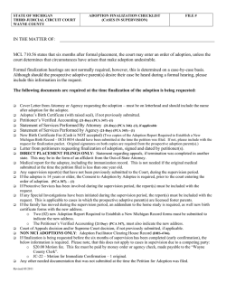

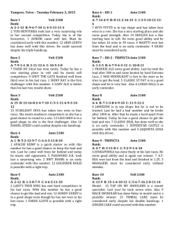

© Copyright 2026