
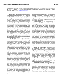
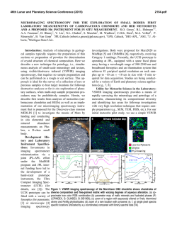
2. BIOSENSOR
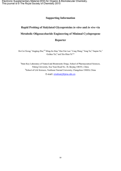
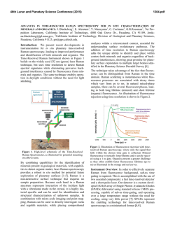
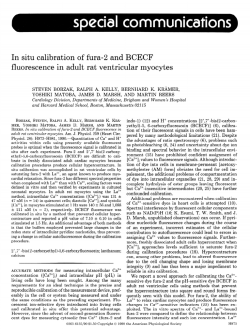
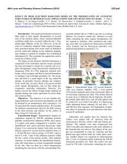
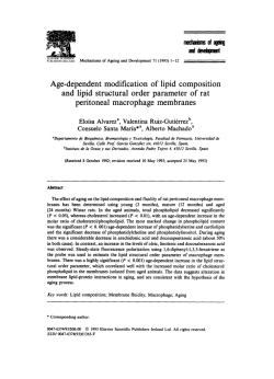
IOSENSOR
2. BSYMPOSIUM
TÜBINGEN 2001
Multi-Parameter Fluorescence Detection at the Single-Molecule Level:
Techniques and Applications
Christian Eggeling
1,2,3
1
1
1
2
2
, Jörg Schaffer , Andreas Volkmer , Claus Seidel , Leif Brand , Stefan Jäger ,
2
Karsten Gall
1
MPI biophys. Chemie, Am Fassberg 11, 37077 Göttingen
2
Evotec OAI, Schnackenburgallee 114, 22525 Hamburg
3
corresponding author ([email protected]
www.evotecoai.com)
Introduction
Fluorescence-based assays using single-molecule techniques are evolving into a very important tool
in science. These techniques include not only direct detection and analysis of single-molecule events,
but also spectroscopic analysis through fluctuation methods such as FCS (fluorescence correlation
spectroscopy) or FIDA (fluorescence intensity distribution analysis). What are the advantages of these
techniques and why is fluorescence chosen as the readout?
Scientific theories of molecular interactions and chemical reactions are mainly described on the singlemolecule level. However, our knowledge of the interactions and properties of molecules arose from
experiments on ensembles of molecules. Experiments have been performed over the past few years
to directly monitor single molecules. Do these experiments significantly improve our understanding of
this area ? According to the fundamental tenet of statistical mechanics, the ergodic theorem, the mean
of a physical value is the same regardless of whether the observation is carried out over time from a
single member of an ensemble or over all members at a single point in time. However, this theorem is
only valid in the case that the system is homogeneous, i.e., all members of the ensemble are similar.
Heterogeneity in a system can either be static or by variations in the ensemble characteristics within
the measurement time. In this case, the mean of a physical value measured for a single molecule over
time and its mean measured over the whole ensemble at a single point in time, i.e., single-molecule
and ensemble experiments, disagree. The characterization of such systems demands the direct
observation of single molecules. Therefore, experiments on the single-molecule level are providing
new comprehensive descriptions of molecular and physical properties and processes which are lost in
ensemble measurements. These include, e.g., the determination of distributions of molecular
properties of a heterogeneous system, the exposure of rare events and changes within an ensemble,
the direct identification and quantification of single molecules, or the observation of the temporal
behavior of single molecules and, thus, the direct observation of temporal fluctuations.
Remarkable progress in single-molecule detection methods has been made through the examination
of single ion channels using the patch-clamp technique [1] and also by monitoring single atoms and
molecules with scanning-tunnel-electron- or scanning-atomic-force-microscopy [2,3]. Improvements in
the field of confocal microscopy have opened up the way for the direct detection of single molecules
with optical methods [4-6]. Due to its superior sensitivity to environmental properties and also its multidimensionality, i.e., its ability to provide various simultaneous readouts of parameters such as
intensity, lifetime, anisotropy, and spectral characteristics (multi-parameter fluorescence detection,
MFD), fluorescence has gained major attraction in the field of single-molecule analysis [7-11]. A
number of fluorescent dyes have been detected and identified directly in solution using different
fluorescence parameters [12-19]. Suitable dyes can also be used as labels of biologically significant
molecules such as proteins and nucleic acids and act as reporters of molecular environment and
characteristics. Single-molecule fluorescence-spectroscopy offers new approaches for DNAsequencing [20,21] as well as the direct resolution of conformational dynamics, binding interactions,
and cleavage reactions of biological molecules [10,22,23] leading, e.g., to superior understanding of
protein functions. Optical methods of single-molecule detection are not confined solely to fluorescence
techniques. Notable successes also include Raman-spectroscopy [24], which can reveal very rare
events that are undetectable using conventional ensemble measurements [25].
Further widespread scientific methods like fluorescence correlation spectroscopy (FCS) use
fluctuations in a fluorescence signal to obtain information on the molecular level of the observed
system. The ability of confocal microscopy to observe fluctuations from single molecules resulted in
fluctuations of sufficient magnitude to make these methods more generally accessible. Thus, FCS,
which was introduced in 1972 [26,27] and temporally analyses the fluctuations by calculating the
correlation function, has evolved into a widespread analysis tool in a wide range of scientific
applications [28-31]. Recently, another powerful method, fluorescence intensity distribution analysis
(FIDA), has been introduced, which analyses the fluorescence fluctuations on the basis of the
distribution of their amplitudes [32,33]. FIDA is not only already applied to particular biological casts
but has also been further developed by using, e.g., the multi-parameter readouts of the fluorescence
(two-dimensional fluorescence intensity distribution analysis (2D-FIDA) [34] and fluorescence intensity
multiple distribution analysis (FIMDA) [35]). Due to their short acquisition times of down to one second
and their fast analysis algorithms with fundamentally solved theoretical descriptions, these fluctuation
methods have become useful in industrial applications. Therefore, FCS and FIDA have found
widespread application in pharmaceutical research and in biotechnology, particularly in drug-discovery
(high-throughput-screening (HTS)) [36-38].
This article will give an overview of fluorescence techniques and applications of single-molecule
detection and analysis. It is focused on the detection of fluorescence emitted from freely diffusing
molecules in solution. A confocal microscope is described, which uses special electronics for detection
and enables the observation of fluorescence emission from single molecules along with monitoring of
various fluorescence parameters (MFD). In the first part, procedures such as the detection and
identification of single molecules, the monitoring of rare events, the direct temporal observation of
binding events and conformational dynamics, as well as the possibility of selective spectroscopy of
molecular states are described. Industrial applications such as HTS are illustrated by a description of
using fluctuation methods such as FCS and FIDA to resolve characteristic properties of biological
assays, e.g., ligand-protein and -vesicle binding or enzymatic reactions.
Set-up: confocal fluorescence microscope
(a) Optical set-up: To study the fluorescence emission from single molecules in solution a standard
confocal epi-illuminated fluorescence microscope is used as shown in Fig.1A and previously described
in detail [34,39,40]. A pulsed or continuous-wave (cw), linearly-polarized laser is coupled into a
microscope objective and focused into the sample. The size of the focus, usually larger than about
0.5 µm, is set by a telescope in front of the microscope. The sample, a highly diluted aqueous dye or
-8
dye labeled biomolecule solution (< 10 M), is placed either on objective slides with a cover glass or in
microscope glass bottom micro- or nanotiter-plates (8- to 2080-wells). Diffusion of a fluorescent
molecule through the laser focus leads to excitation and fluorescence emission of the dye. The
fluorescence is collected by the same objective and imaged onto a pinhole (diameter > 30 µm
depending on the focal size) by the tubelense. Using polarized and/or dichroic (DB) beamsplitters with
up to four detectors (avalanche photodiodes) the detected fluorescence light can be split up into its
different polarization directions (parallel and vertical polarized with respect to the polarization of the
laser) and/or fluorescence emission bands (e.g., fluorescence light above and below 620 nm).
Interference filters (IF) in front of the detectors block unwanted background light due to, e.g., scattering
of the solvent.
signal intensity F(t) / kHz
500
400
B
300
200
100
0
0
20
40
60
80
100 120 140 160 180 200
time t / ms
signal intensity F(t) / kHz
150
C
100
50
0
0
10
20
30
40
50
time t / ms
A
Fig. 1 (A) Standard confocal epi-illuminated fluorescence microscope used for multi-parameter
fluorescence detection at the single-molecule level. (B-C) Multi-Channel-Scaler (MCS) traces
-12
of Rhodamine 6G in water measured at the set-up of (A) (dye concentrations of 10
M (B)
-9
as used in SMD experiments and 5×10 M (C) as applied in fluctuation measurements);
signal intensity F(t) (number of photons detected in time windows of 1 ms (A) and 0.1 ms(B))
against the measurement time t.
(b) Data acquisition electronics: The electronics (multi-parameter fluorescence detection, MFD, in
Fig.1A), are capable of simultaneously recording several parameters of the detected fluorescence
signal: (1) the detector number of each detected photon representing its spectral range or emission
band, λ (e.g., green (< 620 nm) and red ( > 620 nm)), or polarization with respect to the polarization of
the exciting laser light (parallel, ||, or vertical, ⊥); (2) in the case of pulsed laser excitation light the
arrival time, ∆τ, of the signal photon relative to the incident laser pulse, measured by TCSPC (time
correlated single photon counting) to determine the fluorescence lifetime, τ, in an arrival time
histogram (picosecond to nanosecond time scale) either for each detector separately or for a set of
detectors (Fig.2B); (3) the inter-photon time, ∆t, of a signal photon to the preceding signal photon
(millisecond time range) (for details see [8,22,25,39,40]); (4) a multi-channel-scaler (MCS) trace, which
is obtained by counting the number of detected photons within consecutive time windows of constant
size (e.g., 1 ms, Fig. 1B and C) either for each detector separately or for a set of detectors. This is
either done by a separate electronic PC-card [34,39,40] or by software calculation using the interphoton time, ∆t [22,25]. The MCS trace represents the time dependent fluorescence signal intensity,
F(t), on the macroscopic time scale.
Data processing for multi-parameter fluorescence detection (MFD)
The principles of two multi-parameter fluorescence methods at the single-molecule level will be
presented here;
(A) The direct observation of single molecules (single molecule detection, SMD) is only possible in
-11
samples with fluorescent molecule concentrations below 10
M. The mean number of fluorescent
molecules in the detection volume is far below one, i.e., fluorescence bursts above the
background signal level indicate single fluorescing molecules diffusing through the detection
volume. The MCS trace in Fig.1B shows the time dependent fluorescence signal of such an
experiment with the background signal due to Raman scattering from the solvent being solely
detected most of the time and some signal peaks indicating the fluorescence bursts from singlemolecule transits. An important step in analyzing a SMD experiment is to distinguish between
fluorescence and background. It is important to confine the analysis to the actual fluorescence
photons in the burst, avoiding inclusion of extraneous background photons. Burst selection can be
realized using the inter-photon time, ∆t, information as outlined in Fig.2A. The inter-photon time,
∆t, between two consecutive detected background photons is very large, whereas fluorescence
photons emitted during a dye transit cause a photon burst and thus have a small inter-photon
time, ∆t. In the case that the inter-photon times of a certain number of consecutive photons
(depending on the experiment, e.g., 150) are all below a chosen threshold value (horizontal line in
Fig.2A), this photon interval is classified as fluorescence burst and subject for further analysis. For
details see [22,25,39,40].
(B) Fluctuation methods like FCS and FIDA process an entire data stream. They require signal
fluctuations of sufficient amount. The amplitudes of these fluctuations are inversely dependent on
the concentration of fluorescent molecules and are maximum at SMD concentrations as is
apparent in the MCS traces of Fig.1B and C. However, concentrations around 1 nM are sufficient
for such measurements, i.e., the mean number of fluorescent molecules in the detection volume is
around one to ten. There is no constraint that the mean number of fluorescent molecules in the
detection volume must be far below one as in SMD experiments. For FCS, a correlation function is
calculated from the time dependent fluorescence signal, F(t), as shown in Fig.2C [26-31]. This can
either be performed by a separate electronic PC-card [15,34,39] or determined from the MCS
trace by software calculation [22,25,39,40]. In FIDA the distribution of the amplitudes of the MCS
trace (usually with a time window of 40 µs) is determined in a frequency histogram as illustrated in
Fig.2D [32,33]. This is either set up by software from the MCS trace [25] or directly by an
electronic PC-card [32]. Further extension to 2D-FIDA and FIMDA is also possible. In this case, a
joint frequency histogram of the synchronized amplitudes of the MCS traces from two detectors or
multiple frequency histograms of the amplitudes of MCS traces with different time windows are
0.01
excitation
pulse
15000
B
fluorescence
lifetime
10000
5000
0
2
4
6
8
10
arrival time ∆τ / ns
1.4
mean diffusion
time τdiff
1.3
C
1.2
1.1
concentration
1.0
10
-3
10
-2
10
-1
10
0
1
10
correlation time t / ms
logarithmic scale
A
1E-3
0
5000
10000
photon number
15000
Number of events
∆ t / ms
0.1
20000
correlation G(t)
Number of events
produced, respectively, as described in detail in [34,35].
D
10000
1000
100
10
1
0
2
4
6
8
10
12
14
number of photon events
Fig. 2 (A) Inter-photon times, ∆t, of detected photons of the Rhodamine 6G measurement of Fig.1B
together with a threshold value (horizontal line) for burst selection (for a better representation
the ∆t-values are averaged by applying a LEE-filter [39,40]). Representative example data of
(B) fluorescence lifetime analysis (FLA, arrival time histogram together with instrumentresponse function/excitation pulse), (C) fluorescence correlation spectroscopy (FCS,
correlation curve), and (D) fluorescence intensity distribution analysis (FIDA, frequency
histogram of fluorescence intensity amplitudes).
Multi-parameter fluorescence detection (MFD) in single-molecule detection (SMD)
As outlined before SMD searches for fluorescence signal (bursts) above the background signal level.
Each burst is caused by the diffusion of a single molecule through the detection volume. Therefore,
the fluorescence photons of each burst reflect the properties of the corresponding single molecule.
SMD uses various fluorescence parameters (MFD) to obtain as much information as possible in order
to characterize the different single molecules of a sample. In principle, two analysis methods are
possible. (1) Burst integrated analysis determines the fluorescence parameters from all detected
fluorescence photons of a burst. Hence, this method was formerly introduced as burst integrated
fluorescence lifetime (BIFL) [18,22,25,39,40]. This procedure enables identification and quantification
of the different molecule species in a sample and a means of directly exposing the heterogeneity of
the sample. (2) Real-time monitoring obtains the different fluorescence parameters consecutively for a
certain number of fluorescence photons detected in succession throughout the burst and, thus,
registers the time dependent variations of these parameters for one molecule [22,39,40]. This method
directly reveals molecular changes due to, e.g., conformational changes or binding events in real-time.
MFD, i.e., the determination of the fluorescence parameters of a single molecule or of a set of
detected fluorescence photons of a single molecule are determined as followed. (A) The fluorescence
intensity is given by the ratio of the number of photons and the time-interval in which they are detected
as obtained by the corresponding inter-photon times, ∆t. (B) The fluorescence lifetime, τ, is obtained
by fitting a theoretical model to the arrival time (∆τ) histogram (Fig.2B) of these photons. The
theoretical model includes the convolution of the exponential decay, exp(- τ/∆τ), with the instrumentresponse-function of the laser pulse, while fitting is done using the Maximum-Likelihood method
[15,16]. (C) The fluorescence anisotropy, rF, is calculated from the number of photons, N|| and N⊥,
registered on the two detectors monitoring the polarization directions (parallel and vertical polarized
with respect to the polarization of the laser) respectively; rF = [N|| - N⊥] / [N|| + 2 N⊥]. Further factors are
introduced, which correct for the slightly different detection efficiencies, as well as for contributions of
background scattering light and have been described in detail [19]. Through the Perrin-equation, the
anisotropy depends on the rotational correlation time, ρ, as well as the fluorescence lifetime, τ, and
reveals the rotational diffusion characteristics of the fluorescent molecule. In an advanced fit to the
arrival time (∆τ) histograms of the photons from the two detection channels the rotational correlation
time, ρ, can also be obtained directly [19]. (D) In the case that two different fluorescent labels are used
and their different fluorescence emission bands monitored simultaneously, the ratio of the numbers of
photons detected on each detector is used to check their coincident occurrence or to obtain an
efficiency of fluorescence resonance energy transfer (FRET) from one dye to the other [40-43]. This
aids investigation of inter- or intra-molecular distances and, thus, monitoring of binding events to
specific binding sites or conformational changes [23,40-43].
SMD: identifying and quantifying single molecules by burst integrated analysis
After selecting the bursts or single-molecule events as outlined above, one or several fluorescence
parameters can be used to identify a molecule. In Fig.3A-C an example is given using fluorescence
lifetime. Three different samples were investigated in a water/glycerin (60/40 weight percent) mixture;
(A) 6 pM Rhodamine B, (B) 2 pM Rhodamine 6G, and (C) a 1:3 mixture of (A) and (B) for an about
equal-molar (1.5 pM) mixture of both dyes. Fluorescence bursts containing more than 50 signal
photons were selected as single-molecule events and their fluorescence lifetime determined. Fig.3A-C
shows the distribution of the fluorescence lifetime values with their mean values and widths. In the
case of the mixture (C) two distributions are obtained, which show the ability of SMD together with the
determination of fluorescence lifetime to distinguish whether a burst has been caused by one or
another molecule. However, the overlap of both distributions reveals the uncertainty or possible error
probability of the identification, which in this case is 4.7 %. This means, 4.7 % of all bursts were
assigned to the wrong molecule. In order to decrease this error probability, an additional parameter,
like the anisotropy, rF, or the intensity, F, can be taken into account (MFD) as has been shown in
several impressive examples [19,39,40,44,45]. Furthermore, the width of the distribution of the
fluorescence parameters can directly reveal heterogeneities of the sample, since the expected
standard deviations of a fluorescence parameter determination are know beforehand [15,19,40].
These heterogenities signify the presence of different molecular species or states due to different
fluorescence characteristics.
A
0.08
C
B
15
0.06
number of events
probability density
0.10
0.06
0.04
0.04
0.05
0.02
0.02
0.00
0
1
2
3
4
5
6
τ / ns - bin width 0.1 ns
0.00
1
2
3
4
5
τ / ns - bin width 0.1 ns
6
10
5
0
1
2
3
4
5
50
100
150
200
250
50
100
150
200
250
10
5
0
0.00
D
0
0
burst size / number of photons
6
τ / ns - bin width 0.1 ns
Fig. 3 (A-C) Distribution of fluorescence lifetime values determined from single-molecules of (A)
Rhodamine B (6 pM, 394 single-molecule events), (B) Rhodamine 6G (2 pM, 375 singlemolecule events), and (C) a 1:3 mixture of (A) and (B) for an about equal-molar mixture of
both dyes (1.5 pM, 325 single-molecule events) (solvent water/glycerin mixture, 60/40 weight
percent) together with a Gaussian fit to the data ((A) τ = 2.4 ± 0.3 ns, (B) τ = 3.7 ± 0.6 ns, (C)
τ = 2.3 ± 0.4 ns and τ = 3.8 ± 0.5 ns). (D) Distribution of the burst sizes (i.e., number of
photons from one single-molecule event) from sample (C) for Rhodamine B classified
molecules (τ <2.85 ns, upper graph) and Rhodamine 6G classified molecules (τ >2.85 ns,
lower graph) (dots) together with a fit of the theoretical model (line) to the data resulting in
values of the mean number of molecules in the detection volume; Rhodamine B 0.028,
Rhodamine 6G 0.022 (for details see [18]).
The easiest way to quantify a certain molecule species is to count its associated single-molecule
events. This has been addressed elegantly using a flow system with a detection volume covering its
full width [8,20,21,44,46]. In this case, every molecule crosses the detection volume in approximately
the same time and with approximately the same fluorescence emission intensity. The burst sizes are
Poissonian distributed around a mean value. Every single-molecule transit can be assigned to a
fluorescence burst of reasonable size [46]. Such a set-up has, therefore, been taken as fundamental
standard for DNA-sequencing approaches using SMD [20,21]. However, observing free diffusing
molecules in an open detection volume leads to all kinds of bursts from single molecules as becomes
obvious from Fig.1B. The transit of a molecule can occur at the margins of the volume, where low
excitation intensity combined with a short dwell time result in low fluorescence emission. In contrast,
maximum fluorescence emission occurs by a transit through the center of the volume with the
maximum excitation intensity and a long dwell time. The burst sizes have an exponential-like
distribution as shown in Fig.3D. The previously described burst selection, with the demand of a
minimum number of detected photons per burst results in many single-molecule transits being
neglected. Quantification is therefore performed by fitting a theoretical model to the incomplete
experimental burst size distribution (Fig.3D) [18,40]. This model considers the distribution of dwell
times, the inhomogeneous excitation profile, and extrapolates to small burst sizes. In this way, the
quantification of the different species of the dye mixture in Fig.3C can be performed elegantly (Fig.3D)
and checked by FCS and corresponding dilution steps [18].
time [ms]
650
652
6
A
5
5
4
3
3
2
2
1
1
anisotropy rF
4
0
150
75 40
20
0
MCS
30
60
lifetime τ [ns]
648
6
0
648
650
652
time [ms] - time window 1 ms
Fig. 4 Real-time monitoring of single-molecule transits; Rhodamine 6G labeled DNA double-strand
(label-5’-d(CAA AGC GCC ATT CGC CAT TC) and complementary strand 5’-d(GAA TGG
CGA ATG GCG CTT TG), 5 pM in sodium-phosphate buffer, pH 7.5). (A) Fluorescence
parameter trace of a single-molecule transit determined from sets of 150 photons (lifetime, τ,
and anisotropy, rF, with projected frequency distributions, and intensity as MCS-trace). (B)
Two-dimensional parameter diagram obtained from the parameter traces of 976 singlemolecule transits with the corresponding one-dimensional frequency projections. (C-D)
Selective fluorescence lifetime analysis of photons selected from island (I) (C) and island (II)
(D) with fit to data using more than one exponential decay constant and resulting in
amplitudes and decay constants; (C) 10%-4.0 ns, 35%-1.6 ns, 37%-0.5 ns, background
18 % and (D) 84%-4.4 ns, 6%-0.6 ns, background 10 %.
SMD: real-time monitoring of a single-molecule transit
As outlined above, the time dependence of the different fluorescence parameters can be monitored by
consecutive determination from a fractional set of successively detected fluorescence photons within
the single-molecule transit [22,39,40]. This is shown in Fig.4A, where pairs of the fluorescence
parameters lifetime, τ, and anisotropy, rF, have successively been determined for sets of 150 photons
throughout a fluorescence burst caused by a Rodamine 6G labeled double-stranded oligonucleotide
(sequence and sample conditions see figure legend). The corresponding information is obtained from
the inter-photon times, ∆t, and, thus, the macroscopic time of the median fluorescence photon of each
set. In spite of noise fluctuations originating from the uncertainty of the parameter determination, a
clear jump between two levels (τ = 2 ns to τ = 5 ns) is observed for the fluorescence lifetime. To check
whether fluctuations reveal molecular changes, the time-dependent information from all singlemolecule transits have to be gathered. This is done in two-dimensional parameter diagrams, which
plot the frequency of pairs of lifetime, τ, and anisotropy, rF, and of lifetime, τ, and intensity, F, values
together for all photon sets and for all single-molecule transits. Fig.4B shows the two-dimensional
parameter diagrams of 1358 single-molecule events of the double-stranded oligonucleotide. Two
molecular species or conformational states are clearly denoted by the two “islands”; (I) a quenched
state with mean values of F = 100 kHz, rF = 0.2, and τ = 1.4 ns and (II) an unquenched state with
mean values of F = 300 kHz, rF = 0.16, and τ = 4.1 ns (for comparison, measurements of a pure
Rhodamine 6G sample reveal one species with mean values of F = 320 kHz, rF = 0.02, and τ = 4.0 ns
(data not shown) [40]). However, the direct observation of the change between the states shown in
Fig.4A succeeded in only a few single-molecule transits, since the kinetics (correlation time constant of
t = (8.2 ± 1.0) ms, determined by FCS measurements using an extremely expanded excitation volume
- data not shown [40]) are slower than the average diffusion time of the molecules (about 2 ms in the
SMD experiments). Furthermore, the widths of the distributions of the fluorescence parameters of the
two states (e.g., lifetime τ(I) = (1.41 ± 0.3) ns and τ(II) = (4.1 ± 1.1) ns) are larger than expected from
theory [15,19,40] (e.g., lifetime determination using 150 photons (1.41 ± 0.17) ns and (4.1 ± 0.45) ns).
This reveals heterogeneities due to possible sub-states within the two macroscopic states. Here, the
powerful potential of multi-parameter fluorescence SMD is highlighted, since it is the only method with
which it is possible to further analyze the two macroscopic states separately by using state-selective
spectroscopy. In state-selective spectroscopy only those sets of 150 photons, which are assigned to
one specific macroscopic state or species, i.e., whose according fluorescence parameters lie within
one of the “islands” of the two-dimensional parameter diagrams, are selected for further analysis.
Here, sets of photons with a fluorescence lifetime, τ < 2.5 ns, were assigned to the quenched state (I)
and with τ > 3.0 ns to the unquenched state (II). Possible analysis methods are state-selective FCS,
FIDA, or lifetime analysis. Fig.4C-D shows for example the frequency histograms of the arrival times,
∆τ, of the selected photons of states (I) (Fig.4C) and (II) (Fig.4D) together with the lifetime analysis.
Both decays had to be fitted using more than one exponential decay constant (see figure legend),
which reveals the lifetime values of the sub-states. Combining all results and comparing them with the
analysis of similar oligonucleotides (e.g., a labeled single-stranded oligonucleotide exhibiting only one
molecular species with mean values of F = 250 kHz, rF = 0.11, and τ = 4.5 ns (data not shown) [40])
the following model can be proposed for the double-stranded oligonucleotide. (1) Conformational
changes do occur between two macroscopic stable states with a time constant of about 8 ms. These
are due to fluctuations of the position of the labeling dye with basically two different environments;
state (I) interaction with the terminal DNA-base-pair guanine-cytosine (G-C) with specific quenching of
the Rhodamine 6G fluorescence by guanine via photo-induced proton-coupled electron transfer [47]
and state (II) proximity to the next positioned DNA-base-pair adenine-thymidine (A-T) leading to a
slightly enhanced fluorescence lifetime due to interaction with adenine (τ = 4.3 ns) [48]. (2) Both states
reveal sub-states with different interaction efficiencies due to variations in the positions of the dye. In
case of state (I) the dye seems to cover the top of the terminal base-pair, while state (II) reveals
heterogeneities due to sliding of the dye within the major groove of the DNA.
This example is only supposed to be an introduction into the possibilities of multi-parameter
fluorescence detection (MFD) using SMD and has, therefore, not been covered in detail. The full study
would overstretch this tutorial report and is described in detail elsewhere [39,40]. Furthermore, it
includes more possibilities of real-time monitoring of single-molecule transits such as the direct
resolution of reaction kinetics by correlation analysis of the individual fluorescence parameter traces
[22,25,39].
SMD: conclusion
The application of multi-dimensional fluorescence detection (MFD) to SMD enhances the accuracy of
the identification, quantification and, thus, the characterization of a sample, as well as the possibilities
of resolving molecular dynamics and states. This opens up new approaches in all scientific fields such
as analytical chemistry with the detection of rare sample components and impurities, and biophysics
due to the potential for much higher sensitivity in monitoring of molecular reactions, e.g., protein
functions. State-selective spectroscopy is particularly a powerful tool which helps to find better
understandings of molecular states and is only accessible via multi-dimensional fluorescence SMD.
Recent results of experiments applying fluorescence resonance energy transfer (FRET) to SMD have
extended the potentials of this technique [40-43]. However, some problems must still be kept in mind.
As in all fluorescence microscopy applications the maximum number of detectable fluorescence
photons is limited by the photodestruction of the dyes which has already been subject of several
studies [49,50]. The minimum and maximum time resolution of real-time monitoring is given by the
restricted minimum number of photons needed for a fluorescence parameter determination of
sufficient statistical accuracy and also by the limited dwell time of the single molecules as outlined
above, respectively. In the applications presented here, this ranges about from 0.5 µs to 5 ms. In the
field of pharmaceutical applications such as HTS the minimization of the data acquisition and analysis
time is one of the most important issues. SMD experiments like those presented here demand an
acquisition time of at least several seconds to minutes at minimum, since a reasonable amount of
single-molecule events have to be gathered to reach a sufficiently high accuracy. Therefore,
applications for HTS purposes apply other analysis methods based on fluctuation methods which
combine slightly higher molecule concentrations with much lower data acquisition times.
Fluorescence fluctuation methods: applications in biotechnology
Biotechnology fluorescence applications such as HTS necessitate special considerations for both data
acquisition and analysis. In high-performance drug discovery, HTS is used to test libraries of 10,000 to
1,000,000 potential drug candidates for biological reactivity rather than designing a special drug for a
specific biological target. Possible screening targets include the inhibition of binding events, the
activation of protein function, and the control of enzymatic reactions. In HTS as many samples as
possible are tested in the shortest possible time with the smallest possible fraction of false
classifications of the drug candidates. Therefore, besides an efficient read-out mode such as
fluorescence, that is sensitive enough to distinguish, e.g., bound from unbound molecules, HTS
requires short data acquisition times down to one second and analysis methods with the highest
possible statistical accuracy. These requirements are fulfilled by fluorescence fluctuation methods.
The analysis of fluorescence signal fluctuations opens up the possibility of resolving and quantifying
components of a sample with different fluorescence or molecular characteristics; e.g., brightly
fluorescing particles give rise to high fluorescence emission and detection rate, whilst slowly diffusing
fluorescing molecules remain in the detection volume and emit fluorescence over a long period of
time, additionally the fluorescence fluctuations from high concentrated molecules show much smaller
amplitudes than low concentrations of molecules as shown in Fig.1B+C. Thus, the highest possible
statistical accuracy for the characterization of a biological target is reached and is furthermore
increased by the simultaneous measurement of a variety of fluorescence parameters (MFD). In
contrast to SMD, these methods use the whole signal data stream to extract the information and the
necessary data acquisition times can be lowered down to below one second. However, as outlined
above, the analysis demands fluctuations of a certain amplitude, i.e., the concentration of fluorescing
molecules has to be close to the single-molecule level. Several different analysis methods have
evolved over the last few years that are capable of this molecular resolution. They are summarized
below.
A) FCS (fluorescence correlation spectroscopy) analyses the temporal characteristics of fluorescence
fluctuations. The calculated correlation function (Fig.2C) of these fluctuations decays with time
constants that are characteristic of the molecular processes causing these fluorescence changes,
e.g., diffusion into and out of the detection volume and reaction kinetics [26-31]. The amplitude of
the decay is related to the molecular concentration while the inflection point represents the mean
diffusion time, τdiff, of the fluorescing molecules through the detection volume, which is solely
dependent on the diffusion coefficient. Hence, FCS is able to resolve components of a sample
with different diffusion coefficients due to, e.g., different molecular mass. For example, the binding
of a dye labeled peptide to a larger protein is followed by an increase in the mean diffusion time,
τdiff. In this way, biological assays can easily be developed for HTS applications [36,38]. However,
for measurement times as short as one second and for an increasing background signal, the
correlation curves become severely noise limited. Thus, for these conditions, FCS loses its
accuracy. Due to this problem, further fluctuation methods have been developed for HTS.
B) FIDA (fluorescence intensity distribution analysis) relies on a collection of instantaneous values of
the fluctuating fluorescence intensity by building up a frequency histogram of the signal amplitudes
throughout a measurement (from the according MCS trace as outlined above) [32,33]. The
resulting distribution of signal intensities is then analyzed by a theory which relates specific
fluorescence brightness, q (intensity per molecule in kHz), and absolute concentration, c (mean
number of molecules in the detection volume), of the molecules under investigation as well as
possible background signal due to scattering or impurities. FIDA distinguishes species of the
sample according to their different values of specific molecular brightness, q. Reactions resulting
in the quenching of the fluorescence emission of a dye-label or in the aggregation of dye labeled
molecules can easily be monitored applying FIDA. Possible HTS applications have been
introduced by enzyme cleavage [32] as well as inhibition of ligand binding to acceptor proteins
exposed on vesicle surfaces [37]. Since FIDA is based on a solely statistical process (i.e., building
up of a histogram) rather than on a numerical operation (i.e., calculating the correlation function as
in the case of FCS), FIDA is able to maintain good statistical accuracy down to acquisition times of
one second.
C) 2D-FIDA (two-dimensional fluorescence intensity distribution analysis) and FIMDA (fluorescence
intensity multiple distribution analysis) are based on extensions of the FIDA technique resulting in
improved performance. 2D-FIDA is applied to a two-detector set-up monitoring either different
polarization or emission bands of the fluorescence signal (as described above) and in addition to
the FIDA performance achieves additional molecular resolution by the concurrent determination of
two specific brightness values of each detection channel, q1(channel1) and q2(channel2) [34]. By
observing the molecular resolved fluorescence anisotropy simple and more complex binding
events and enzymatic reactions may be followed. Alternatively, such events may be followed by
labeling with two dyes with different fluorescence emission bands and combining this with either
two-color excitation by different lasers or FRET interaction. Thus, use of a second detector can
improve the power of FIDA to distinguish between molecular components and is, therefore,
increasingly applied in high-performance drug discovery [38]. In contrast, FIMDA only demands
one detection channel (as outlined above) and extracts all characteristics of both FCS and FIDA
(diffusion time, τdiff, specific molecular brightness, q, and absolute concentration, c) from a single
measurement [35]. FIMDA increases the readout and improves likelihood of molecular resolution
of different components of the sample effectively by one dimension. Its viability and improvements
in comparison with FIDA have been supported by measurements characterizing a real proteinligand interaction [35].
D) Fluorescence lifetime analysis (FLA) is not a fluctuation method but also a method, which is
capable of distinguishing components of a sample through variation in fluorescence
characteristics. By analyzing the arrival time histogram, ∆τ (obtained by TCSPC as described
above, Fig.2B), of all detected signal photons of a measurement, a molecular species may be
characterized by its fluorescence lifetime, τ, and allows the determination of molecular signal
count rates, cq, as well as the consideration of background signal. FLA can be applied to any
biological reaction exposing a change in the fluorescence lifetime (due to environmental changes
of the dye-label, such as a quenching reaction) as shown in Fig.5A for a peptide-protein
interaction. Here, a high statistical accuracy is still obtained even though data acquisition times are
below one second. This fulfills the demands for its operational use in biotechnology techniques
such as HTS. Since FLA does not demand signal fluctuations of a particular amount, it can be
employed at any concentration range.
Fig.5B+C reveals the powerful possibilities of the fluctuation methods in the field of HTS or analytical
sciences. Here, the inhibition of a peptide-protein interaction is monitored using 2D-FIDA. The
anisotropy of the binding complex is determined with and without the presence of fluorescence
impurities. Fluorescence background is a major problem in HTS due to the possibility of intrinsic
autofluorescence of the investigated drug candidates. When the anisotropy is determined from the
overall signal as is usually the case in fluorescence experiments, its values are erroneous due to the
presence of a background signal (Fig.5B). The inclusion of an autofluorescent component and
calculation of the molecular resolved anisotropy of the binding complex by 2D-FIDA is capable of the
readout correction (Fig.5C).
0.30
A
2.8
2.6
0.26
0.24
0.22
0.20
0.18
0.16
2.4
B
0.30
0.28
2.2
2.0
1.8
10
-6
10
-5
10
-4
10
-3
10
-2
10
-1
10
0
10
concentration Calmodulin [µM]
1
10
2
anisotropy
lifetime τ / ns
3.0
0.28
anisotropy
3.2
0.26
0.24
0.22
0.20
0.18
0.16
C
0.01
0.1
1
10
100
conc inhibitor [µM]
1000
Fig. 5 (A) Binding of a small MR121-labeled peptide to the protein Calmodulin monitored by
fluorescence lifetime analysis (FLA, 0.5 s measurement time, error bars result from 10
measurements); change of the overall lifetime upon titration of the protein. Hyperbolic fit
(line) to the data results in a binding constant, KD =19.5 ± 1.4 nM. (B-C) Binding of a small
Cyanin5-labeled peptide to the SH2-domain of the Grb2-protein monitored by a change of
the fluorescence anisotropy, rF (10 s measurement time, error bars result from 10
measurements); titration of unlabeled peptide inhibitor with (open dots) and without (black
dots) addition of impurities (1 µM Rhodamine 800). Determination of the anisotropy from the
overall signal (B) and from 2D-FIDA (C) resolving the fluorescence signal from the labeled
peptide and the impurities. For more details on the assay system see [35].
As can be seen from the applications introduced above, fluctuation methods are not only useful for
HTS but may also be widely applied for monitoring all kinds of molecular interactions in the life
science, for example diagnostic purposes, SNP (single nucleotide polymorphism) analytic, chip
technologies, or even material, e.g., semiconductor surface characterization.
References
The authors thank Dr. Mary Cole for critically reading the manuscript
References
[1]
Sakmann, B. and Neher, E. (1995) Single-Channel Recording. Plenum Press, New York
[2]
Binnig, G., Rohrer, H., Gerber, C. and Weibel E. (1982) Phys.Rev.Lett., 49, 57-60
[3]
Ludwig, M., Rief, M., Schmidt, L., Li, H., Oesterhelt, F., Gautel, M. and Gaub, H.E. (1999) AFM, a tool for singlemolecule experiments. Appl.Phys.A, 68, 173-176
[4]
Hirschfeld, T. (1976) Optical microscopic observation of single small molecules. Appl.Opt., 15, 2965-2966
[5]
Moerner, W.E. and Kador, L. (1989) Optical detection and spectroscopy of single molecules in a solid. Phys.Rev.Lett.,
62, 2535-2538
[6]
Orrit, M. and Bernard, J. (1990) Single pentacene molecules detected by fluorescence excitation in a p-terphenyl
crystal. Phys.Rev.Lett., 65, 2716-2719
[7]
Eigen, M. and Rigler, R. (1994) Sorting single molecules: Application to diagnostics and evolutionary biotechnology.
Proc.Natl.Acad.Sci.U.S.A., 91, 5740-5747
[8]
Keller, R.A., W.P. Ambrose, P.M., Goodwin, J.H., Jett, J.C., Martin and Wu, M. (1996) Single-molecule fluorescence
analysis in solution. Appl.Spectrosc., 50, 12A-32A
[9]
Plakhotnik, T., E.A. Donley, and Wild, U.P. (1997) Single-molecule spectroscopy. Annu.Rev.Phys.Chem., 48, 181-212
[10]
Xie, X.S. and Trautman, J.K. (1998) Optical studies of single molecules at room temperature. Annu.Rev.Phys.Chem.,
[11]
Ambrose, W. P., Goodwin, P.M., Jett, J.H., van Orden, A., Werner, H.J. and Keller, R.A. (1999) Single Molecule
[12]
Shera, E.B., Seitzinger, N.K., Davis, L.M., Keller, R.A. and Soper, S.A. (1990) Detection of single fluorescent
49, 441-480
Fluorescence Spectroscopy at Ambient Temperature. Chem.Rev., 99, 2929-2956
molecules. Chem.Phys.Lett., 174, 553-557
[13]
Soper, S.A., Davis, L.M. and Shera, E.B. (1992) Detection and identification of single molecules in solution.
J.Opt.Soc.Am.B, 9, 1761-1769
[14]
Mertz, J., Xu, C. and Webb, W.W. (1995) Single-molecule detection by two-photon-excited fluorescence. Opt.Lett. 20,
2532-2534
[15]
Zander, C., Sauer, M., Drexhage, K.H., Ko, D.S., Schulz, A., Wolfrum, J., Brand, L., Eggeling, C. and Seidel, C.A.M.
(1996) Detection and characterization of single molecules in aqueous solution. Appl.Phys.B, 63, 517-523
[16]
Brand, L., Eggeling, C., Zander, C., Drexhage, K.H. and Seidel, C.A.M. (1997) Single-molecule identification of
coumarin-120 by time-resolved fluorescence detection - comparison of one- and two-photon excitation in solution.
J.Phys.Chem.A, 101, 4313-4321
[17]
Müller, R., Zander, C., Sauer, M., Deimel, M., Ko, D.S., Siebert, S., Arden-Jacob, J., Deltau, G., Marx, N.J., Drexhage,
K.H. and Wolfrum, J. (1996) Time-resolved identification of single molecules in solution with a pulsed semiconductor
diode laser. Chem.Phys.Lett., 262, 716-722
[18]
Fries, J.R., Brand, L., Eggeling, C., Köllner, M. and Seidel, C.A.M. (1998) Quantitative identification of different single-
[19]
Schaffer, J., Volkmer, A., Eggeling, C., Subramaniam, V., Striker, G. and Seidel, C.A.M. (1999) Identification of single
[20]
Ambrose, W.P., Goodwin, P.M., Jett, J.H., Johnson, M.E., J.C. Martin, Marrone, B.L., Schecker, J.A., Wilkerson,
molecules by selective time-resolved confocal fluorescence spectroscopy. J.Phys.Chem.A, 102, 6601-6613
molecules in aqueous solution by time-resolved fluorescence anisotropy. J.Phys.Chem.A, 103, 331-336
C.W., Keller, R.A., Haces, A., Shih, P.J. and Harding, J.D. (1993) Application of Single Molecule Detection to DNA
Sequencing and Sizing. Ber.Bunsenges.Phys.Chem., 97, 1535-1542
[21]
Dörre, K., Brakmann, S., Brinkmeier, M., Han, K.T., Riebeseel, K., Schwille, P., Stephan, J., Wetzel, T., Lapczyna, M.,
Stuke, M., Bader, R., Hinz, M., Seliger, H., Holm, J., Eigen, M. and Rigler, R. (1997) Techniques for single molecule
sequencing. Bioimaging 5, 139-152
[22]
Eggeling, C., Fries, J.R., Brand, L., Günther, R. and Seidel, C.A.M. (1998) Monitoring conformational dynamics of a
single molecule by selective fluorescence spectroscopy. Proc.Natl.Acad.Sci.U.S.A., 95, 1556-1561
[23]
Weiss, S. (1999) Fluorescence spectroscopy of single biomolecules. Science, 283, 1676-1683
[24]
Kneipp, K., Kneipp, H., Itzkan, I., Ramachandra, R.D. and Feld, M.S. (1999) Ultrasensitive Chemical Analysis by
Raman Spectroscopy. Chem.Rev., 99, 2957-2975
[25]
Eggeling, C., Schaffer, J., Seidel, C.A.M., Korte, J., Brehm, G., Schneider, S. and Schrof, W. (2001) Multidimensional
Surface Enhanced Resonance Raman Spectroscopy of Single Dye Molecules on Single Ag-Particles. J.Phys.Chem.A,
105, 3673-3679
[26]
Magde, D., Elson, E.L. and Webb, W.W. (1972) Thermodynamic fluctuations in a reacting system - measurement by
[27]
Ehrenberg, M. and Rigler, R. (1974) Rotational Brownian motion and fluorescence intensity fluctuations. Chem.Phys.,
[28]
Thompson, N.L. (1991) Fluorescence Correlation Spectroscopy. In Topics in Fluorescence Spectroscopy, Volume 1:
[29]
Widengren, J. and Rigler, R. (1998) Review - fluorescence correlation spectroscopy as a tool to investigate chemical
fluorescence correlation spectroscopy. Phys.Rev.Lett., 29, 705-708
4, 390-401
Techniques. Lakowicz. J.R., editor. Plenum Press, New York. 337-378
reactions in solutions and on cell surfaces. Cell.Mol.Biol., 44, 857-879
[30]
Visser, A.J.W.G. and Hink, M.A. (1999) New perspectives of fluorescence correlation spectroscopy. J.Fluoresc., 9, 8187
[31]
Fluorescence Correlation Spectroscopy Theory and Applications, Rigler, R. and Elson, E.s., editors, Chemical Physics
Springer (2001)
[32]
Kask, P., Palo, K., Ullman, D. and Gall, K. (1999) Fluorescence-intensity distribution analysis and its application in
biomolecular detection technology. Proc.Natl.Acad.Sci.U.S.A., 96, 13756-13761
[33]
Chen, Y., Müller, J.D., So, P.T.C. and Gratton, E. (1999) The Photon Counting Histogram in Fluorescence Fluctuation
Spectroscopy. Biophys.J., 77, 553-567
[34]
Kask, P., Palo, K., Fay, N., Brand, L., Mets, Ü., Ullman, D., Jungmann, J., Pschorr, J. and Gall, K. (2000) Two-
[35]
Palo, K., Mets, Ü., Jäger, S., Kask, P. and Gall, K. (2000) Fluorescence Intensity Multiple Distribution Analysis:
Dimensional Fluorescence Intensity Distribution Analysis: Theory and Applications. Biophys.J., 78, 1703-1713
Concurrent Determination of Diffusion Times and Molecular Brightness. Biophys.J. 79
[36]
Auer, M., Moore, K.J., Meyer-Almes, F.J., Günther, R., Pope, A.J. and Stoeckli, K.A. (1998) Fluorescence correlation
[37]
Schaertl, S., Meyer-Almes, F.J., Lopez-Calle, E., Siemers, A. and Kramer, J. (2000) A novel and robust homogeneous
spectroscopy: lead discovery by miniaturized HTS. DDT, 3, 457-465
fluorescence-based assay using nanoparticles for pharmaceutical screening and diagnostics. Journal of Biomolecular
Screening, 5, 227-237
[38]
Ullmann, D., Busch, M. and Mander, T. (1999) Fluorescence correlation spectroscopy-based screening technology.
Inn.Pharm.Tech., 30-40
[39]
Eggeling, C., Berger, S., Brand, L., Fries, J.R., Schaffer, J., Volkmer, A. and Seidel, C.A.M. (2001) Data registration
[40]
Eggeling, C. (2000) Analyse von photochemischer Kinetik und Moleküldynamik durch mehrdimensionale
[41]
Ha, T., Enderle, T., Ogletree, D.F., Chemla, D.S., Selvin, P.R. and Weiss, S. (1996) Probing the interaction between
and selective single-molecule analysis using multi-parameter detection. J.Biotechnol., 86, 163-180
Einzelmolekül-Fluoreszenzspektroskopie. Dissertation, Georg-August Universität Göttingen
two single molecules: Fluorescence resonance energy transfer between a single donor and a single acceptor.
Proc.Natl.Acad.Sci.U.S.A., 93, 6264-6268
[42]
Deniz, A.A., Dahan, M., Grunwell, J.R., Ha, T.J., Faulhaber, A.E., Chemla, D.S., Weiss, S. and Schultz, P.G. (1999)
Single-pair fluorescence resonance energy transfer on freely diffusing molecules: Observation of Förster distance
dependence and subpopulations. Proc.Natl.Acad.Sci.U.S.A., 96, 3670-3675
[43]
Ha, T.J., Ting, A.Y., Liang, J., Caldwell, W.B., Deniz, A.A., Chemla, D.S., Schultz, P.G. and Weiss. S. (1999) Singlemolecule fluorescence spectroscopy of enzyme conformational dynamics and cleavage mechanism.
Proc.Natl.Acad.Sci.U.S.A., 96, 893-898
[44]
van Orden, A., Machara, N.P., Goodwin, P.M. and Keller, R.A. (1998) Single-Molecule Identification in Flowing
[45]
Herten, D.P., Tinnefeld, P. and Sauer, M. (2000) Identification of single fluorescenctly labeled mononucleotide
Sample Streams by Fluorescence Burst Size and Intraburst Fluorescence Decay Rate. Anal.Chem. 70, 1444-1451
molecules in solution by spectrally resoved time-correlated single-photon counting. Appl.Phys.B-Lasers&Optics, 71,
765-771
[46]
Enderlein, J., Robbins, D.L., Ambrose, W.P., Goodwin, P.M. and Keller, R.A. (1997) Statistics of single-molecule
detection. J.Phys.Chem.B, 101, 3626-3632
[47]
Seidel, C.A.M., Schulz, A. and Sauer, M.H.M. (1996) Nucleobase-Specific Quenching of Fluorescent Dyes. 1.
Nucleobase One-Electron Redox Potentials and Their Correlation with Static and Dynamic Quenching Efficiencies.
J.Phys.Chem., 100, 5541-5553
[48]
Fries, J. R. (1998) Charakterisierung einzelner Moleküle in Lösung mit Rhodamin-Farbstoffen. Dissertation,
[49]
Eggeling, C., Widengren, J., Rigler, R. and Seidel, C.A.M. (1998) Photobleaching of Fluorescent Dyes under
[50]
Eggeling, C., Widengren, J., Rigler, R. and Seidel, C.A.M. (1999) Photostabilities of fluorescent dyes for single-
Universität-Gesamthochschule Siegen
Conditions used for Single-Molecule-Detection: Evidence of Two-Step Photolysis. Anal.Chem., 70, 2651-2659
molecule spectroscopy: Mechanisms and experimental methods for estimating photobleaching in aqueous solution. In
Applied fluorescence in chemistry, biology and medicine. Rettig, W., Strehmel, B., Schrader, M. and Seifert, H.,
editors, Springer, Berlin, 193-240


© Copyright 2026