
Structural reforms, macroeconomic fluctuations and income
SERIE
REFORMAS ECONÓMICAS
39
STRUCTURAL REFORMS,
MACROECONOMIC
FLUCTUATIONS AND INCOME
DISTRIBUTION IN BRAZIL
Marcelo Neri
José Márcio Camargo
LC/L.1275
November de 1999
This document was prepared by Marcelo Neri researcher of Instituto de Pesquisa Econômica Aplicada (IPEA) and José
Márcio Camargo, professor of the Economic Department PUC/Rio, for the project “Growth, Employment and Equity:
Latin America in the 1990s” (HOL/97/6034). The views expressed in this document, which has been reproduced
without formal editing, are those of the authors and do not necessarily reflect the views of the Organization.
CONTENTS
ABSTRACT................................................................................................................................................. 5
I. INTRODUCTION.................................................................................................................................. 7
PART A. PORTRAITS OF REFORMS AND INCOME DISTRIBUTION........................................ 9
II. ANALYSIS OF REFORMS................................................................................................................. 9
1. ECONOMIC BACKGROUND ................................................................................................................... 9
1.1 Stabilization .................................................................................................................................. 9
1.2 Trade opening................................................................................................................................ 10
2. DATING REFORMS ................................................................................................................................ 10
III. TEMPORAL EVOLUTION OF INCOME DISTRIBUTION ............................................................ 15
1. DESCRIPTION OF PESQUISA NACIONAL DE AMOSTRAS A DOMICILIO – PNAD.......................................... 15
2. INCOME CONCEPTS AND UNITS OF ANALYSIS .......................................................................................... 15
3. TEMPORAL EVOLUTION OF INEQUALITY............................................................................................ 16
IV. INCOME DISTRIBUTION DECOMPOSITIONS........................................................................ 19
1. THEIL INDEX DECOMPOSITION ........................................................................................................... 19
1.1 Gross rates of contribution ......................................................................................................... 22
1.2 Marginal rates of contribution.................................................................................................... 22
1.3 Gross and Marginal Contributions: Robustness Analysis................................................................... 26
V. THE IMPACT OF REFORMS ON THE RICHES......................................................................... 27
1. AGGREGATE ABSOLUTE IMPACT........................................................................................................ 27
2. PROFILE OF THE IMPACT OF THE REFORMS ON THE RICHES....................................................................... 28
3. INEQUALITY DECOMPOSITION EXERCISES ......................................................................................... 33
3.1 The top 10%.................................................................................................................................. 34
3.2 University Graduates .................................................................................................................... 35
PART B. DYNAMIC ASPECTS OF INCOME DISTRIBUTION ..................................................... 39
VI. REFORMS, STABILIZATION AND INCOME DISTRIBUTION ............................................. 39
1.
2.
3.
4.
DESCRIPTION OF PESQUISA MENSAL DO EMPREGO – PME .............................................................. 39
AN UPDATED ASSESSMENT OF INEQUALITY ...................................................................................... 39
PME LONGITUDINAL ASPECT AND INEQUALITY COMPARISONS........................................................ 40
OTHER DISTRIBUTIVE IMPACTS OF STABILIZATION ........................................................................... 42
4
VII. MACRO DETERMINANTS OF INCOME DISTRIBUTION:
A TIME SERIES APPROACH ...................................................................................................... 53
1.
2.
3.
4.
5.
INCOME DISTRIBUTION DETERMINANTS ............................................................................................ 53
UNEMPLOYMENT ............................................................................................................................... 59
INFLATION ......................................................................................................................................... 60
REAL INTEREST RATES ....................................................................................................................... 60
MINIMUM WAGES .............................................................................................................................. 61
VIII. CONCLUSIONS............................................................................................................................. 65
BIBLIOGRAPHY..................................................................................................................................... 71
STATISTICAL ANNEX .......................................................................................................................... 73
NOTES ..................................................................................................................................................... 77
5
ABSTRACT
This paper attempted to measure the evolution of income distribution and its determinants during
the period of economic reforms. The paper was divided in two parts: in the first and main part of
the paper, long-run relations between reforms and income distribution were explored. The
second part of the paper explored relations between movements of distributive variables, on the
one hand, and economic reforms and macroeconomic fluctuations, on the other.
First, we attempted to study the impact of the economic reforms on the riches. First, we
assessed absolute income changes in the top 10% of the income distribution assessing how the
composition of this group changed during the reform period. We also assessed how much of the
changes in inequality observed between pre-reform and post-reform periods comes from changes at the
10% richest. While the absolute contribution of the 10% richest to total inequality is extremely high in
Brazil, there is not much evidence to suggest that it has increased over the period of the reforms. In the
1990-93 period this contribution in the case of the economically active population has risen from 79.5
to 83.5 then fall to 81.7 in 1997. It is interesting to note that the peak of the series was found in 1976.
The second channel analyzed here is the skill-differential between the high school group
and the rest of the labor force. One of the reasons why this breakdown is of interest is the
evidence that growth is increasingly skill-intensive. The analysis of the profile of the 10% richest
stresses the importance of general human capital explanatory power: 7.83% of the population has
12 or more years of education while the share of this group among the rich corresponds to 44%
and 61% when one take into account the extension of the rich group income. This last statistic
was 53% in 1990 which indicates a sharp effect of the reforms on the composition of the riches
towards highly educated groups. In the period of reforms 1990-97, the rate of return to primary
and secondary education levels falls while the rate of return on university degree rises steeply.
The third distributive channel emphasized here is the effect of stabilization on inequality
measures, specially those operating through changes in the volatility of individual income. We
used PME the micro-longitudinal aspect of PME in two alternative ways: first, the 4 consecutive
observations of the same individuals were treated independently. The second way took earnings
average across four months before inequality measures were calculated.
The main result obtained is that the post-stabilization fall of inequality measures is 2 to 4
times higher on a monthly basis that is traditionally used in Brazil than when one uses mean
earnings across four months. Another way of looking at these effects of stabilization on
inequality measures is to note that most of the fall of the inequality measures is attributed to the
within groups component in the monthly inequality measures. Overall, the main point here is that
most of the monthly earnings inequality fall observed after stabilization may be credited to a
reduction of earnings volatility and not to a fall in permanent earnings inequality.
7
I. INTRODUCTION
Brazil is not only a late-comer in terms of structural reforms and stabilization but major institutional
changes observed during the last 11 years did not point towards the so-called New Economic Model
(NEM). In particular, while all major Latin American economies were moving towards sounder fiscal
apparatus and more flexible labor regulation schemes, the Brazilian Constitution of 1988 introduced
many obstacles to the NEM on both accounts.
On the other hand, liberalization of international trade started with the Collor administration in
1990 and were intensified with Cardoso administration in 1994. Similarly, domestic financial reforms,
liberalization of the capital account and privatization were implemented rather late in comparison with the
rest of the continent but at least they are in line with the NEM.
Complementarily, the impacts of the reforms implemented by Collor and Cardoso on income
distribution were dominated by changes in the macroeconomic environment (inflationary instability, deep
recession, stabilization boom and external crisis). It is not a trivial exercise capturing the impacts of
economic reforms. For instance, the overlapping of the post-Constitution period with the period after the
external opening of the economy does not allow us to identify which impulses drove the rather sharp
increase in labor productivity observed (i.e. increased labor costs or increased exposure to competition).
This paper attempts to measure the evolution of income distribution and its determinants during
the period of economic reforms. Our point of departure is to establish few conceptual points: first, the
movement towards reforms is not unidirectional in Brazil and many institutional changes occurred
simultaneously. This creates difficulties in the assessment of distributive effects of specific reforms.
Second, there has been a rather long lag before the idea of doing reforms gets momentum in the country.
Fernando Henrique Cardoso 1995-98 first term administrative record will be more known as a period of
consolidating stabilization rather than of reforms implementation. The peak of the first generation of
reforms is only now becoming visible in Brazil. In this sense an analysis of the effects of Brazilian
reforms on income distribution must include updated data and a prospective component. Third, the
permanent fall of inflation observed after the Real plan should be treated as an economic reform given its
effects on economic behavior and institutions. Finally, the effects of macroeconomic fluctuations in
Brazilian distributive variables is so prominent that it can not be left out of the analysis.
The paper is divided in two parts: in the first part, long-run relations between reforms and income
distribution are explored. The main empirical strategy pursued here is to establish comparisons between
reform related institutional characteristics and income distribution aspects at different points in time. The
contrasts between portraits observed before and after reforms were launched allows tentative
interpretations of casual relations between implemented reforms and distributive outcomes.
8
In order to set key days in terms of reforms implementation, we use indexes of institutional
reforms found in the literature (Morley et all (1999) and Lora (1997)) and other types of evidence (section
2). The main reforms measured are related to the following fields: trade, labor, tax, financial, capital
account and privatization. The change of inflationary regime in 1994 is perceived as a separate reform.
On the income distribution side, we use national level information extracted from PNAD
household surveys to construct aggregate inequality measures (section 3) and to apply standard
decomposition techniques (section 4). These exercises are performed for different definitions (income
concepts, population concepts and inequality measures) calculated for the following years: 76, 85, 90, 93
and 97. The 1976-90 period is used as evidence of the pre-reform period while the proposed reform period
(1990-97) occupy the central role in the analysis. The reform period is divided in two parts: the 1990-93
initial period of reforms and inflationary instability and the 1993-97 period where the effects of the new
round of reforms implemented, including stabilization, are assessed.
In the end of the first part of the paper, we attempt to study the impact of the economic reforms on
the riches (section 5). First, we analyze absolute income changes in the top 10% of the income distribution.
At this point we also assess how the composition of this group changed during the reform period. Second,
we assess the contribution of this group and the university graduates group to overall inequality.
The second part of the paper explores PME monthly household surveys to extract relations
between movements of distributive variables, on the one hand, and economic reforms and
macroeconomic fluctuations, on the other. It qualifies the effects of the 1994 stabilization on income
distribution (section 7). First, it takes advantage of the higher degrees of freedom provided PME in
comparison with PNAD to choose dates before and after stabilization income distribution comparisons
are performed. For instance, PME allows to measure the moment just before the launching of the
stabilization plan and compare it with the end of 1998, incorporating the effects of the adverse external
that hit recently the Brazilian economy. Second, the fact that PME follows the same individuals across
short periods of time allows to qualify the nature of changes of inequality observed. In particular, the
longitudinal aspect to PME allows to disentangle the effects of lower inflation rates on temporal earnings
variability from those exerted on stricto sensu inequality measures (and its between groups and within
groups components).
Given the occurrence of sharp macroeconomic fluctuations in the Brazilian case and the
possibility of measuring various aspects of income distribution in a detailed manner with PME, the final
part of the paper attempts to isolate distributive effects of macro shocks and policies. The possibility of
constructing for the 1980-99 period monthly series of specially tailored variables according to individual
and family records of PME allow us to apply standard time series techniques capturing the effects of
macro variables on labor earnings distribution variables (section 7). We analyze the correlation patterns
between macro variables (unemployment, inflation, various types of exchange rates, interest rates and
minimum wages) and distributive variables (aggregate inequality measures and mean earnings of
different groups (by years of schooling, age, household status, sector of activity and working class).
9
PART A. PORTRAITS OF REFORMS AND INCOME DISTRIBUTION
Part A assesses the long-run impacts of reforms on income distribution in Brazil. It performs
comparisons between reform related institutional characteristics and income distribution aspects
at different points in time. The contrasts between portraits observed before and after reforms were
launched allows tentative interpretations of casual relations between implemented reforms and
distributive outcomes. We start setting an economic background for the implementation of
reforms. The second step is to identify key dates in terms of reform implementation. These points
are used to study the effects of reforms on income distribution.
II. ANALYSIS OF REFORMS
1. Economic background
Amongst Latin American countries, the experience of Brazil has been quite peculiar in the sense
that reforms, and in particular trade liberalization, only started a few years ago. Whereas other
countries in the region started opening their economies in the early and mid-1980’s, in Brazil the
process started effectively in the early 1990’s. With stabilization, the story is the same. Whereas
Mexico started its stabilization process in the mid-80’s and Argentina in the early 1990’s, in
Brazil only in 1994 successful price stabilization was achieved. In the early 1990’s two major
changes have taken place. First, the opening of the economy. Second, the launching of a
successful stabilization plan in 1994. The structural changes introduced with trade liberalization
and stabilization are so significant to explain the macroeconomic environment and the dynamic
of other reforms implementation that it is inevitable to focus the present analysis on these events.
1.1 Stabilization
Since at least the early 1980’s, inflation became the central policy issue in Brazil. Three major
stabilization efforts were attempted since then: the Cruzado plan in 1986, the Collor plan in 1990
and the Real plan in 1994. The first two plans failed. The Real plan has been very successful in
bringing down inflation and the prospects in this respect are very good even after the waves of
external shocks that hit the Brazilian economy in September, 1997 (Asian crisis), September,
1998 (Russian crisis) and the January, 1999 exchange rate fluctuation.
The Real plan of 1994 had at least two major differences in comparison with previous plans.
First, a very successful process of “de-indexation” based on the establishment of a transitory unit of
account fully indexed to inflation. The second difference in relation to previous plans was that the
10
economy was considerably more open and the government was prepared to let the currency appreciate.
As a consequence, imports played the role of the adjustment variable between aggregate demand and
domestic aggregate supply and the nominal exchange rate established a ceiling for prices, at least in the
tradable sector. The opening of the economy and the appreciation of the Real are two central elements in
what is so far seen as a very successful stabilization effort. Trade liberalization helped the stabilization
and, at the same time, it is seen by the government as a key element in the new development strategy. The
enormous impact on the balance of payments is the subject of the following section.
1.2 Trade opening
Besides perhaps stabilization, the most important element of the reforms is the opening of the economy.
Until 1990 Brazil was a very closed economy. This resulted from a deliberate strategy of import
substitution and, due to the debt crisis in the 1980’s, from the pressures to produce trade surpluses. Since
the early 1990’s the environment has changed. On the one hand, the international context has changed
with the return of foreign credit. On the other, there is a widely shared view that the closeness of the
economy and the active trade and industrial policies of the 1980’s were an hindrance to price stability and
sustained growth. The debt crisis of the 1980’s imposed a severe external constraint on the Brazilian
economy. The drastic reduction of foreign credit and the increase in interest services on the external debt
required the creation of trade surpluses. The exchange rate became pegged to the rate of inflation and
imports were gradually reduced with the increase of tariff and non-tariff barriers.
Since 1985 the trade surplus varied between US$ 8 billion (1986) and US$ 19 billion (1988). On
average, between 1985 and 1994, it surpassed the mark of US$ 10 billion. Trade surpluses were roughly
enough to balance the current account until 1994. Trade liberalization starts formally in the late 1980’s but
more effectively in the early 1990’s but its most dramatic effects show up after 1994 with the expansion
of domestic demand and the appreciation of the Real. There were two episodes of currency appreciation.
The first, in 1989-90, is associated with the rapid acceleration of inflation and, to a certain extent, can be
seen as “involuntary”. The second episode, in 1994-5, however was used as an instrument of the
stabilization strategy. The government deliberately let the nominal exchange rate appreciate in order to
increase the competitive pressure on the prices of tradable.
Until mid-1994 the average monthly trade surplus was around US$ 1.1 billion. The surpluses
turned into deficits in 1994. Imports of intermediary and capital goods increased roughly 150% between
1992-3 and 1995-6 and imports of consumption goods increased 300%. In the period 1993-95 GDP grew
around 15% which gives an idea of the increase in the import coefficient.
2. Dating reforms
In terms of measuring the timing of institutional reforms we use estimates found in Morley and all (1999)
and Lora (1997). The reforms measured are related to the following fields: trade, labor, tax, financial,
capital account and privatization. Each index is normalized to be between zero and one, with one being
the most reformed or free from distortion or government intervention. Graphs 1.A. to G. present a
comparison for various indexes of reforms in Brazil with a simple average of 17 Latin America countries.
Tables 1A to E present evidence of specific reforms and some of its direct effects on economic variables.
11
Graph 1
A - General
1.0
0.8
0.6
0.4
0.2
Brazil
1994
1992
1990
1988
1986
1984
1982
1980
1978
1976
1974
1972
1970
0.0
Average
Source: Morley et all (1999)
B - Capital Account Reforms
C - Privatization
1.0
1.0
E - Tax Reforms
1990
1988
1986
1994
D - Trade Reforms
1992
Source: Morley et all (1999)
1994
Source: Morley et all (1999)
1984
1982
1980
1978
1976
1974
1970
1994
1992
1988
1990
Brazil
Average
1992
Brazil
1986
1984
1982
1980
1978
0.0
1976
0.2
0.0
1974
0.4
0.2
1972
0.6
0.4
1970
0.6
1972
0.8
0.8
Average
Brazil
Average
Brazil
Source: Morley et all (1999)
Source: Morley et all (1999)
F - Financial Reforms
G - Labor Reforms
1.0
1.0
0.8
0.8
0.6
0.6
0.4
0.4
0.2
0.2
1990
1988
1986
1984
1982
1980
1978
1976
1974
1970
1994
1992
1990
1988
1986
1984
0.0
1982
0.2
0.0
1980
0.4
0.2
1978
0.4
1976
0.6
1974
0.6
1972
0.8
1970
0.8
1972
1.0
1.0
Average
Brazil
Average
1995
1994
1993
1992
1991
1990
1989
1988
1987
1986
1994
1992
1990
1988
1986
1984
1982
1980
1978
1976
1974
1972
1970
Brazil
Source: Morley et all (1999)
1985
0.0
0.0
Average
Source: Lora (1997)
Before the analysis proceeds it should be noted that besides inevitable imperfections
included in these indexes from the view of specific countries, it presents a very good perspective
of the main relative trends observed. Graph 1.A presents the simple average across five reforms
(it excludes labor reforms). Brazil that was more liberalized than the other countries in the region
in the begin of the series, stagnated during the 70s and 80s, falling slightly behind given the
12
generalized movement towards reforms in the region then observed. The average regional reform
index rises by 50% during the 1970-90 period. In the end of the1980s, Brazil engages in a
serious reform catch-up effort. In a period of three years starting in 1988, the general Brazilian
reform index rises 40%. The analysis of individual reforms components reveals that financial
reforms, trade reform and tax reforms are the main determinants of this jump. The upward trend
continues until the end of the period of analysis and beyond. The index rises from 0.74 to 0.81 in
the last three years.
It is important now to make a few qualifications about the general reform index in Brazil.
First, it attributes equal weights to the different reforms considered while some aspects of
reforms are clearly more important than others. Trade liberalization is probably more important
for income distribution purposes than other reforms considered. The problem is that the trade
reform index only incorporates tariffs practices in the calculations (average level and dispersion)
and perhaps the most important international trade related reform observed in the Brazilian was
the abandonment of quantitative restrictions beginning in 1990. So if one incorporates these
restrictions in the analysis and a greater weight to international trade as well, Brazil would be
less liberalized before 1990 and the size of the jump observed in this year would be magnified.
A second problem of the general Brazilian index used is to attribute zero weights to labor
and social security reforms which have rather important distributive consequences. Labor and
social security went through a counter-reform with the 1988 Constitution. The labor reform
index presented in graph 1.G illustrate the in labor legislation reversal.
A final related problem is that the general index also not considered the inflationary
environment and its pervasive effects on income distribution. The 1987-94 period was
characterized by high and instable inflation rates which produced decisive influences on
economic behavior and institutions. For example, as Table1.A shows annual inflation rates that
were 475% in 1991, reached a peak of 2489% in 1993 falling to 9.1% in 1996. The coefficient of
variation follows a similar movement 3.86 in 1991, 20.03 in 1994 and 0.41 in 19961 2. Once
again, the result would be to neutralize at least in part the jump towards liberalization observed
in 1988. By the same token, the permanent fall of inflation observed in 1994 after the Real plan
should be treated as a key economic reform.
In sum, our perception is that once the end of quantitative restrictions on international
trade occurred in 1990, the labor and social security counter-reforms observed in 1988 and the
inflationary environment is considered there would remain two decisive dates in the reforms
implementation path in Brazil: 1990 and 1994.
13
Table 1
A. STABILIZATION
Annual inflation rate level
Variability of monthly inflation rates 1
Temporal real earnings variability 2
Nominal wage rigidity 3
1
Coefficient of variation within year
2
Variance of Log real earnings across 4 consecutive months
3
Percentage of fixed wages between 2 consecutive months
1991
475.10
1996
9.10
Peak Value
2,489.10
Date Peak Source
1993
CPI - IBGE
3.86
0.41
20.03
1994
CPI - IBGE
0.1206
0.1060
0.1363
1994
PME Longitudinal
24.8
30.7
32.25
1995
PME Longitudinal
B. TRADE REFORM
Weighted Average Nominal Protection Rate
1991
27.4
1996
11.5 *
Peak Value Date Peak Source
27.4
1991
H. Kume (IPEA, 1996)
Labor Productivity Index
100
144.2
144.2
1996
Mercado de Trabalho, IPEA
Exchange Rate Versus the US$
77
61*
77
1991
World Bank data files
Real Effective Exchange Rate1
83
59
91
1992
World Bank data files
C. FISCAL REFORM
Net Debt of the Public Sector - Internal (% of GDP)
1991
12.6
1996
30.3
Peak Value Date Peak Source
30.3
1996
Fabio Giambagi (BNDES, 1996)
Net Debt of the Public Sector - External (% of GDP)
24.5
4.0
24.5
1991
Public Investment (% of GDP)
2.6
2.2
3.4
1993
Boletim Conjuntural, IPEA
Public Domestic Savings - excluding enterprises (% of GDP)
3.2
-1.4
3.4
1994
Pinheiro e Giambiagi (1997)
Boletim, Central Bank
D. FINANCIAL REFORMS (DOMESTIC AND CAPITAL ACCOUNT) AND PRIVATIZATION
Private Investment (% of GDP)
1991
16.2
1996
16.8
Private Savings (% of GDP)
15.2
17.1
18.6
1995
Pinheiro e Giambiagi (1997)
External Savings (% of GDP)
0.4
3.3
---
1996
Pinheiro e Giambiagi (1997)
Net Capital Flows (in US$ millions)
897
32895.0
---
1996
BNDES
1988.1
4749.8
---
1996
Central Bank
4
11
14
1992
BNDES
Flows of Privatization Revenues (in US$ millions)
No. of Enterprises Privatized
Peak Value Date Peak Source
16.8
1996
Boletim Conjuntural, IPEA
E. TAX REFORM
Total tax burden (% of GDP)
1991
25.2
1996
28.9
Peak Value Date Peak Source
28.9
1996
SRJ, STN, MPAS, IBGE
Social security tax burden (% of GDP)
5.7
6.6
6.6
1996
Goods and services tax burden (% of GDP)
12.6
13.3
13.3
1996
SRJ, STN, MPAS, IBGE
SRJ, STN, MPAS, IBGE
Income tax burden (% of GDP)
4.2
5.2
5.2
1996
SRJ, STN, MPAS, IBGE
Property tax burden (% of GDP)
0.46
0.9
0.9
1996
SRJ, STN, MPAS, IBGE
Other types of tax burden (% of GDP)
2.2
2.9
2.9
1996
SRJ, STN, MPAS, IBGE
15
III. TEMPORAL EVOLUTION OF INCOME DISTRIBUTION
The biggest advantage of the Brazilian case in this type of study is in terms of data availability. There is a
long established tradition with household surveys. We will focus our empirical analysis in two
geographical dimensions: a) national level; b) six main metropolitan areas. As we move from the national
to the metropolitan level, the availability of updated data increases. We will use as basic data sources two
household surveys: i) PNAD 1976, 1981, 1985, 1990, 1993 and 1997. ii) PME from 1980 onwards. We
start the study using PNAD, PME will be described and used in the second part of the paper.
1. Description of Pesquisa Nacional de Amostras a Domicilio – PNAD
This is a national annual household survey performed in the third quarter that interviews 100,000
households every year. It is conducted by Instituto Brasileiro de Geografia e Estatística - IBGE
since 1967. PNAD underwent a major revision between 1990 and 1992 increasing the size of the
questionnaire from 60 to 130 questions. The new questionnaire is available for 1992, 1993, 1995, 1996
and 1997. The National coverage and the diversity of income sources is the main advantage of using
PNAD here. The change of questionnaire mentioned will impose compatibility efforts and imperfections
in the comparison across time.
2. Income concepts and units of analysis
We will work with two basic inequality measures the Gini coefficient and the Theil-T. The popularity of
the Gini coefficients and the fact that it allows to incorporate null incomes in the analysis justifies its use.
The Theil-T will be the central measure used here given its exact decomposable property. PNAD will be
our main data source in this study. We will analyze the following years: 76, 85, 90, 93, 97.
We will work with the five pairs of population-income concepts using PNAD:
Income Concept
Occupied
Population Concept
Economically
Active
Active Age
Total
Labor NH
Labor
Individuals All sources
Per Capita All sources
We use as benchmark value the Theil-T based on economically active and all income sources.
16
3. Temporal evolution of inequality
Tables 2.A and 2.B presents the Theil-T and the Gini coefficient during the 1976-97 across the
different pairs of population-income concepts. The analysis of the temporal evolution of the
inequality reveals the following features:
i) The 1976-85 period corresponds to the final years of the military regime: fall of inequality in
the 1976-85 period for all concepts used. Our benchmark measure (i.e.; Theil-T based on all
income sources for the economic active population) falls from 0.825 to 0.72 in this interval.
ii) The 1985-90 period is characterized by the absence of reforms and rises in inflationary levels
and volatility induced by the launching of successive failed stabilization attempts which
produced a rise of inequality in the 1985-90 period for all concepts analyzed. Our basic
inequality measure rises from 0.72 to 0.748 during this interval.
Looking at the period before economic reforms 1976-90 as a whole, our basic benchmark
measure falls from 0.825 to 0.748. This downward trend is closed followed by broader inequality
concepts such as those based on the active age population and on total per capita income while
narrower measures based on occupied population shows a very mild upward movement. This
contrast can be partially credited to the increase of female participation in labor markets, as next
section shows.
The 1990-97 is the period of most interest here due to the implementation of economic
reforms. Our benchmark inequality measure (i.e.; economically active and all income sources)
falls from 0.748 to 0.699. This downward movement is followed by all Theil-T measures except
the one for the per capital all income sources concepts. As posed in section 2, the period of
reforms 1990-97 can be further divided into two subperiods.
iii) the 1990-93 period is characterized by the combination of high inflation with economic
reforms: the direction of inequality changes is not robust across the different concepts used. For
example, while our basic measure rises from 0.748 to 0.793, the inequality concept based on the
occupied population-labor income concepts falls. While broader concepts present mild increases.
The difference between broader and narrower inequality concepts may be explained by the
decrease in the participation of young cohorts in labor markets in the begin of the decade which
compensates partially the effects of increased female participation observed in the previous
years.
iv) The 1993-97 period is characterized by the combination of successful stabilization and the
intensification of economic reforms. The result is a fall of inequality for all concepts used. For
example, the measure based on economically active and all income sources falls from 0.793 to 0.699.
Overall, during the 1976-97 period there is a fall of all five population-income pair of
concepts for both inequality measures used. The average Theil-T index across concepts falls
12.6%. The same statistic for the Gini coefficient presents a fall of 2.87% This result is
17
interesting because during the 1976-93 period the inequality fall is not unanimous across
population-income concepts pairs used for both inequality measures. The average Theil-T index
across concepts falls 4.83% in the 1976-93 period which is only 38.3% of the total fall observed
in the 1976-97 period. The same exercise applied to the Gini index yields similar results: a fall of
0.08% in the 1976-93 period which corresponds 28.9% of the total fall observed in the 1976-97
period. In other words, the main part of inequality measures drop observed in Brazil during the
21 years analyzed occurred in the last four years. We believe that this is mostly explained by the
effects of the 1994 stabilization on income distribution. We will return to these issues in section
6 of the paper.
Table 2
A. THEIL-T INDEX - BRAZIL
Population Concept - Income Concept
1976
1985
Occupied - Labor Income
Occupied - Labor Income Normalized b
Economically Active - All Income Source
Active Age - All Income Sources
Total - Per Capita All Income Sources
Source: PNAD
0.795
0.846
0.825
0.850
0.826
0.702
0.772
0.720
0.745
0.698
1990
1993
1997
0.800
0.854
0.748
0.782
0.748
0.771
0.831
0.793
0.791
0.756
0.686
0.809
0.699
0.710
0.715
B. GINI COEFFICIENT - BRAZIL
Population Concept - Income Concept
1976
1985
1990
1993
1997
Occupied - Labor Income
Occupied - Labor Income Normalized b
Economically Active - All Income Source
Active Age - All Income Sources
Total - Per Capita All Income Sources
Source: PNAD
0.595
0.610
0.603
0.609
0.616
0.590
0.608
0.595
0.604
0.590
0.600
0.615
0.605
0.618
0.607
0.596
0.610
0.601
0.600
0.599
0.578
0.602
0.583
0.587
0.595
19
IV. INCOME DISTRIBUTION DECOMPOSITIONS
This section attempts to identify the main structural determinants of Brazilian inequality. As we
saw in the previous section, income distribution according to the several concepts analyzed went
through various changes in the last years. Now, it is necessary to go beyond and to quantify the
close determinants of this evolution. In search of an association between inequality measures, on
the one hand, and the availability, utilization, and return of different factors of production and
personal characteristics on the other, we perform a standard inequality decomposition exercise.
1. Theil index decomposition
T = Σ αg βg Log αg + Σ αg βg Tg
where,
(1)
αg = Yg/µ - Ratio between mean income of group G (Yg) and overall mean income.
βg = ng/N - Share of group G in the total population.
Tg - Theil index of group G.
The first term of expression (1) corresponds to the between groups component while the
second term corresponds to the within groups component. Table 3.A. identifies between and
within groups components for the following subgroups arbitrarily defined: gender, age,
schooling, working class, sector of activity, population density and region.
The different classification criteria used in the table 3 can be aggregated in terms of
variables related to human capital (education and age), physical capital accumulation (sector of
activity and working class), personal characteristics subject to discrimination (sex and race) and
localization (demographic region and population density). Table 3 implements this
decomposition for the economically active population and all income sources concept used as a
benchmark. This table illustrates the different arbitrary chosen categories for each classification
criteria used.
As a specific illustrative example, take the third partition of table 3.A. with the
decomposition when groups are defined according to the educational attainment of individuals.
In terms of the static picture presented for 1997 in the three first columns of table, we see that the
between group component explains 34.7% (0.243/0.699) of the total Theil-T index of 0.699.
20
Table 3
A. THEIL-T INDEX DECOMPOSITION AND VARIATION - BRAZIL
Universe : Economically Active Population - All Income Sources
1997
Total Between Within
Gender
Male
0.602
0.099
0.503
0.097 -0.080 0.177
Female
Total
0.699
0.019
0.680
Race
Indigenous
0.000
0.000
0.000
White
0.667
0.183
0.484
Black
0.010 -0.131 0.141
Yellow
0.022
0.014
0.008
Not specified
0.000
0.000
0.000
Total
0.699
0.066
0.633
Age
Up to 24 years
-0.042 -0.079 0.038
0.130 -0.014 0.144
25 to 34 years
35 to 59 years
0.536
0.146
0.389
More than 60 years 0.076
0.005
0.071
Total
0.699
0.058
0.642
-0.030 -0.046 0.017
0 Years
Schooling
1 to 4 years
0.002 -0.096 0.098
5 to 8 years
0.032 -0.054 0.087
9 to 12 years
0.177
0.050
0.127
13 to 16 years
0.407
0.295
0.111
More than 16 years 0.112
0.094
0.018
Not specified
0.000
0.000
0.000
Total
0.699
0.243
0.456
Unemployed
Working Class
0.001 -0.003 0.003
0.160
0.065
0.095
Public Servant
Formal Employee
0.137 -0.006 0.142
Informal Employee -0.026 -0.083 0.056
Self-Employed
0.140 -0.019 0.159
Employer
0.293
0.204
0.089
Unpaid
-0.004 -0.009 0.005
Not specified
0.000
0.000
0.000
Total
0.699
0.149
0.550
Sector of Activity Agriculture
0.008 -0.056 0.063
0.103
0.007
0.096
Manufacturing
Construction
0.015 -0.012 0.027
Public Sector
0.168
0.066
0.102
Services
0.405
0.036
0.369
0.001 -0.003 0.003
Not specified
Total
0.699
0.039
0.660
Population Density Metropolitan
0.425
0.145
0.280
Urban
0.286 -0.026 0.312
Rural
-0.012 -0.064 0.053
Total
0.699
0.055
0.645
South
Region
0.115
0.009
0.106
South-east
0.463
0.111
0.352
North
0.020 -0.006 0.026
0.035 -0.081 0.116
North-east
Center-west
0.066
0.005
0.061
Total
0.699
0.038
0.661
Source: PNAD
Diff. Between 97 and 90
Total Between Within
-0.071 -0.012 -0.059
0.022
0.006
0.016
-0.049 -0.006 -0.043
0.000
0.000
0.000
-0.028 0.003 -0.031
-0.018 0.000 -0.017
-0.003 -0.002 0.000
0.000
0.000
0.000
-0.049 0.000 -0.048
-0.001 0.015 -0.016
-0.045 -0.022 -0.023
0.006
0.003
0.003
-0.008 -0.004 -0.004
-0.049 -0.008 -0.040
0.001
0.010 -0.009
-0.024 0.002 -0.026
-0.036 -0.011 -0.025
-0.013 -0.018 0.006
-0.007 -0.011 0.004
0.030
0.027
0.003
0.000
0.000
0.000
-0.049 -0.001 -0.048
0.001 -0.002 0.002
0.008
0.009 -0.002
-0.057 -0.009 -0.048
-0.001 -0.003 0.002
0.034
0.017
0.017
-0.029 -0.009 -0.021
-0.005 -0.008 0.003
0.000
0.000
0.000
-0.049 -0.005 -0.044
-0.017 -0.001 -0.016
-0.018 0.004 -0.022
-0.008 -0.002 -0.006
-0.031 -0.013 -0.018
0.025
0.014
0.011
0.001 -0.002 0.002
-0.049 0.000 -0.049
-0.032 0.002 -0.034
-0.023 -0.021 -0.002
0.006
0.014 -0.008
-0.049 -0.004 -0.044
0.006
0.006
0.000
-0.017 0.018 -0.035
-0.015 -0.012 -0.002
-0.010 -0.001 -0.009
-0.013 -0.008 -0.005
-0.049 0.003 -0.051
21
B. THEIL-T INDEX DECOMPOSITION AND VARIATION - BRAZIL
Universe : Economically Active Population - All Income Sources
Diff. Between 76 aand 97 Diff. Between 76 and 90
Total Between Within
Total Between Within
-0.201 -0.026 -0.175
Gender
Male
-0.129 -0.014 -0.116
0.075 0.006 0.069
Female
0.053 0.000 0.052
Total
-0.125 -0.019 -0.106
-0.077 -0.014 -0.063
-0.012 0.029 -0.041
Up to 24 years
Age
-0.011 0.015 -0.026
-0.130 -0.050 -0.080
25 to 34 years
-0.085 -0.028 -0.057
0.001 0.011 -0.011
35 to 59 years
-0.005 0.008 -0.013
More than 60 years 0.016 0.001 0.015
0.025 0.005 0.020
Total
-0.125 -0.009 -0.116
-0.077 -0.001 -0.076
0.011 0.039 -0.028
0 Years
Schooling
0.010 0.029 -0.019
-0.118 -0.010 -0.108
1 to 4 years
-0.094 -0.012 -0.082
-0.130 -0.066 -0.063
5 to 8 years
-0.094 -0.055 -0.039
0.001 -0.029 0.030
9 to 12 years
0.014 -0.010 0.024
0.055 0.030 0.025
13 to 16 years
0.062 0.042 0.021
More than 16 years 0.055 0.046 0.010
0.025 0.018 0.007
0.000 0.000 0.000
Not specified
0.000 0.000 0.000
Total
-0.125 0.010 -0.135
-0.077 0.011 -0.088
0.002 0.002 0.000
Unemployed
Working Class
0.001 0.004 -0.003
0.029 0.024 0.005
Public Servant
0.021 0.015 0.006
-0.163 -0.047 -0.116
Formal Employee
-0.107 -0.039 -0.068
Informal Employee -0.013 -0.008 -0.005
-0.012 -0.005 -0.007
-0.020 0.005 -0.025
-0.054 -0.012 -0.042
Self-Employed
0.045 0.035 0.010
Employer
0.074 0.044 0.030
-0.004 -0.007 0.004
Unpaid
0.001 0.000 0.001
-0.002 0.007 -0.008
Not specified
-0.002 0.007 -0.008
Total
-0.125 0.010 -0.136
-0.077 0.015 -0.092
-0.002 0.037 -0.039
Sector of Activity Agriculture
0.015 0.038 -0.023
-0.078 -0.025 -0.053
Manufacturing
-0.060 -0.029 -0.031
-0.022 -0.006 -0.015
Construction
-0.014 -0.005 -0.009
-0.037 -0.009 -0.028
Public Sector
-0.006 0.004 -0.010
0.019 -0.007 0.027
Services
-0.006 -0.021 0.016
-0.006 -0.005 -0.001
Not specified
-0.007 -0.003 -0.004
Total
-0.125 -0.016 -0.109
-0.077 -0.016 -0.060
-0.156 -0.058 -0.098
Population Density Metropolitan
-0.125 -0.061 -0.064
0.037 -0.004 0.041
Urban
0.060 0.017 0.043
-0.006 0.037 -0.043
Rural
-0.012 0.023 -0.035
Total
-0.125 -0.025 -0.101
-0.077 -0.021 -0.056
South
Region
-0.004 0.010 -0.014
-0.010 0.004 -0.014
South-east
-0.162 -0.022 -0.140
-0.145 -0.040 -0.105
North
0.006 -0.004 0.010
0.020 0.008 0.013
North-east
0.011 0.009 0.002
0.021 0.010 0.011
Center-west
0.023 -0.003 0.026
0.036 0.005 0.031
Total
-0.126 -0.010 -0.115
-0.077 -0.013 -0.064
Source: PNAD
22
The last three columns of table 3.A. presents the changes of these levels observed for
1997 when compared with the begin of the economic reform period in 1990. Most of the
inequality fall of -0.049 (0.699 minus 0.748) observed from the perspective of different
schooling categories proposed is explained by the fall of the within group component of –0.048
(0.456 –0.504). while the between groups component remained almost unchanged –0.001. Table
3.B. allows a similar analysis for the pre-reform and the whole period of analysis.
1.1 Gross rates of contribution
The gross decomposition of the Theil index synthesizes the relative importance of the between
groups term of different criteria used in total inequality. Among all the variables considered,
years of schooling and working classes related classifications are the most explicative (or
contributive) variables for total inequality. Both variables explanatory power increased
substantially during the whole period under analysis (table 3.A). Between 1976 and 1997, the
gross contribution of years of schooling and working class for total inequality increased from
28,2% to 34,7%, and from 16.9% to 21.4%, respectively.
Age, which represents a proxy of human capital accumulation due to the acquisition of
experience, presents the third highest gross contribution in total inequality in 1997 but also an
oscillating pattern across time. Between 1976 and 1990, the gross contribution increases from
8.1% to 8.8%, decreasing in the period after reaching values similar to the begin of the series
8.2% in 1997.
The gender classification presents the lower gross contribution rate for total inequality
and decreased almost monotonically between 1976 and 1997 from 4,6% to 2,7%. The variable
sector of activity also presents a low contribution for total inequality even not considering its
likely interactions with working class. The gross contribution of this variable decreased from
6,7% to 5,2% between 1976 and 1990 but it was slightly increased to 5,6% until 1997.
A behavior similar to the one presented in sector of activity classification is observed
with population density classification falling from 9,7% to 7,9% between 1976 and 1990, and
constant until in 1997 (7,8%). Finally, the classification related to the five main Brazilian regions
shows a more stable behavior with a small decrease in its explicative power between 1976 and
1997, from 5,9% to 5,4%.
1.2 Marginal rates of contribution
In order to take into account interactions between the different classifications to get the marginal
impact of each variable once the other classifications were taken into account, we choose a
smaller set of different classification criteria to be implemented simultaneously. Since the sum of
the gross contribution of the between group components of the three main variables (age,
working class and years of schooling variables) is 64.6% of total inequality while the gross
effects of the other five variables is residual amounting less than 30% of total inequality. We will
be working with the interactions between age, working class and years of schooling variables as
shown in table 3.B.
23
Table 4
A - GROSS RATES OF CONTRIBUTION THEIL-T
Universe : Economically Active Population - All Income Sources
Groups:
Gender
Age
Schooling
Working Class
Sector of Activity
Population Density
Region
Source: PNAD
1976
1985
1990
1993
1997
4.6%
8.1%
28.2%
16.9%
6.7%
9.7%
5.9%
4.9%
9.9%
32.0%
22.3%
5.2%
7.1%
4.6%
3.3%
8.8%
32.6%
20.6%
5.2%
7.9%
4.7%
3.5%
8.0%
30.3%
18.7%
3.7%
5.6%
4.0%
2.7%
8.2%
34.7%
21.4%
5.6%
7.8%
5.4%
B. MARGINAL RATES OF CONTRIBUTION THEIL-T
Universe : Economically Active Population - All Income Sources
Age
Schooling
Working Class
1976
1985
1990
1993
1997
7.1%
25.7%
9.2%
8.0%
25.3%
9.6%
6.8%
26.0%
8.7%
6.2%
23.8%
8.2%
5.9%
26.4%
8.7%
Source: PNAD
The first point to note is that the sum of the marginal contribution to overall inequality produced
by the three classifications choose that in the other four years of the series is fairly stable and do not go
below 41% reaches a rather low value of 38.2% in 1993. A similar phenomenon is also observed when
we use the sum of the gross contributions of the seven classification criteria used reaching a value of
73.8% in 1993 and values always above 80% in the other years. The specially low explanatory power of
between groups components in 1993 may be credited to the high inflationary instability observed what
would magnify the within groups components. We will return to this point in section 6. For now we will
abstract from 1993 in the analysis of table 3.B.
The marginal explanatory power of schooling which by far is the most important variable rises
from 25.7% in 1976 to 26% in 1990, increasing to 26.4 in 1997. The marginal contribution of age, that is
once years of schooling and working class effects were taken into account, decreases slightly from 7.1%
in 1976 to 6.8% in 1990 and then decreases more sharply reaching 5.9% in 1997. Finally, the marginal
working class contribution decreases from 9.2% in 1976 to 8.7% in 1990 and remain on these levels in
1997. In sum, the 1990-97 period that can be characterized by the implementation of reforms in Brazil
presents an increase of the explanatory power of education, a decrease for age while working class
remained on the same levels in the extreme points of the series.
24
Table 5
A. RATES OF CONTRIBUTION THEIL-T - 1997
GROSS RATES
Population Concept
Income Concept
Groups:
Gender
Race
Age
Schooling
Working Class
Sector
Population Density
Region
Occupied Occupied Economically A Active Age Total - Per Capita
Labor NH1
Labor
All Sources
0.6%
8.3%
6.6%
35.0%
16.8%
5.9%
6.9%
4.0%
2.7%
9.4%
7.8%
34.6%
21.0%
5.1%
7.5%
5.4%
2.7%
9.4%
8.2%
34.7%
21.4%
5.6%
7.8%
5.4%
All Sources All Sources
3.3%
8.5%
7.3%
36.0%
19.8%
6.0%
7.5%
4.9%
0.0%
12.1%
0.9%
41.3%
14.2%
10.2%
11.1%
8.3%
MARGINAL RATES
Population Concept
Income Concept
Groups:
Age
Schooling
Working Class
1/ Normalized by Hours
Occupied Occupied Economically A Active Age Total - Per Capita
Labor NH1 Labor All Sources
All Sources All Sources
3.9%
26.6%
5.6%
4.7%
25.7%
8.7%
5.9%
26.4%
8.7%
5.7%
28.0%
8.5%
2.8%
34.9%
5.3%
B. RATES OF CONTRIBUTION THEIL-T - 1993
GROSS RATES
Population Concept
Income Concept
Groups:
Gender
Race
Age
Schooling
Working Class
Sector
Population Density
Region
Occupied Occupied Economically A Active Age Total - Per Capita
Labor NH1 Labor All Sources
All Sources All Sources
1.1%
7.5%
7.0%
34.4%
16.0%
4.9%
6.0%
2.9%
3.5%
3.5%
8.3%
8.3%
7.7%
8.0%
30.0%
30.3%
18.4%
18.7%
3.4%
3.7%
5.5%
5.6%
4.2%
4.0%
MARGINAL RATES
4.2%
7.6%
7.0%
30.5%
17.6%
4.2%
5.4%
3.9%
0.0%
10.8%
0.4%
36.8%
11.9%
7.8%
9.1%
6.9%
Population Concept
Occupied Occupied Economically A Active Age Total - Per Capita
Income Concept
Labor NH1 Labor All Sources
All Sources All Sources
Groups:
Age
4.6%
5.0%
6.2%
6.1%
2.6%
Schooling
26.6%
22.8%
23.8%
24.4%
32.3%
Working Class
5.2%
7.9%
8.2%
8.3%
4.8%
1/ Normalized by Hours
25
C - RATES OF CONTRIBUTION THEIL-T - 1990
GROSS RATES
Population Concept
Income Concept
Groups:
Gender
Race
Age
Schooling
Working Class
Sector
Population Density
Region
Occupied Occupied Economically A Active Age Total - Per Capita
Labor NH1 Labor All Sources
All Sources All Sources
1.4%
7.7%
8.4%
38.1%
24.0%
10.3%
11.5%
4.7%
4.0%
3.3%
8.0%
8.8%
9.3%
8.8%
32.6%
32.6%
26.6%
20.6%
7.8%
5.2%
10.5%
7.9%
5.3%
4.7%
MARGINAL RATES
4.2%
7.9%
7.5%
34.0%
19.3%
6.1%
7.7%
4.6%
0.1%
11.2%
0.2%
40.3%
13.4%
10.3%
13.5%
8.0%
Population Concept
Occupied Occupied Economically A Active Age Total - Per Capita
Labor NH1 Labor All Sources
All Sources All Sources
Income Concept
Groups:
Age
4.7%
5.3%
6.8%
6.5%
2.4%
Schooling
27.6%
23.1%
26.0%
27.5%
34.4%
Working Class
9.4%
12.3%
8.7%
8.9%
4.9%
1/ Normalized by Hours
D. RATES OF CONTRIBUTION THEIL-T - 1985
GROSS RATES
Population Concept
Income Concept
Groups:
Gender
Age
Schooling
Working Class
Sector
Population Density
Region
Occupied Occupied Economically A Active Age Total - Per Capita
Labor NH1 Labor All Sources
All Sources All Sources
2.0%
8.4%
36.7%
20.9%
7.4%
8.2%
3.8%
5.0%
4.9%
9.3%
9.9%
30.9%
30.4%
22.0%
22.3%
5.0%
5.2%
7.0%
7.1%
4.6%
4.6%
MARGINAL RATES
5.9%
8.6%
31.6%
21.4%
6.3%
6.8%
4.4%
0.1%
0.1%
41.5%
15.1%
11.3%
13.6%
8.4%
Population Concept
Occupied Occupied Economically A Active Age Total - Per Capita
Income Concept
Labor NH1 Labor All Sources
All Sources All Sources
Groups:
Age
6.9%
7.3%
8.4%
8.3%
1.9%
Schooling
28.3%
23.9%
24.4%
25.6%
34.0%
Working Class
6.9%
9.4%
9.6%
10.0%
5.2%
1/ Normalized by Hours
26
E - RATES OF CONTRIBUTION THEIL-T - 1976
GROSS RATES
Population Concept
Income Concept
Groups:
Gender
Age
Schooling
Working Class
Sector
Population Density
Region
Occupied Occupied Economically A Active Age Total - Per Capita
Labor NH1 Labor All Sources
All Sources All Sources
2.6%
6.9%
33.9%
15.9%
8.8%
11.4%
5.1%
4.8%
4.6%
7.5%
8.1%
28.6%
28.2%
16.9%
16.9%
6.9%
6.7%
9.8%
9.7%
5.9%
5.9%
MARGINAL RATES
5.1%
7.2%
27.3%
16.0%
6.8%
8.8%
5.8%
0.0%
0.2%
36.6%
12.0%
13.7%
17.6%
10.2%
Population Concept
Occupied Occupied Economically A Active Age Total - Per Capita
Income Concept
Labor NH1 Labor All Sources
All Sources All Sources
Groups:
Age
6.2%
6.4%
7.1%
7.0%
1.6%
Schooling
29.1%
25.3%
25.7%
25.0%
30.6%
Working Class
7.1%
9.2%
9.2%
9.3%
4.9%
1/ Normalized by Hours
1.3 Gross and Marginal Contributions: Robustness Analysis
Table 5 allows to test the difference of gross contribution rates across the five population-income
concepts pairs used for 1997. The comparison of contribution rates between occupied population with
and without controls for hours shows that the explanatory power attributed to gender, race and age
reduces drastically, specially gender, once the effects of partial working hours is taken into account.
The comparison of individual based concepts, take for example the economically active
population, with family based measures, here represented by the per capita income concept classified
according to head of household characteristics shows:
i)
ii)
iii)
iv)
v)
vi)
Gender and age contribution rates falls from 2.7% to zero and 7.3% to 0.9%, respectively.
Race gross contribution rises from 9.4% to 12.1%. This is explained by the high propensity of
marriages within the same race groups.
Similarly, spatial related classifications such as population density and region are also less subject
to marriages of different sorts which reinforces the inequality contribution at family level when
compared with individual level inequality measures.
Age gross and marginal contribution rates decrease when one moves from individual to family
level concepts. Marginal rates of contribution falls from 5.9 to 2.8% when one moves from EAP
to per capita concepts.
Years of schooling gross and marginal contribution rates increase substantially when one moves
from individual to family level concepts. Marginal rates of contribution rises from 26.4 to 34.9%
when one moves from EAP to per capita concepts.
In contrast, working class gross and marginal contribution rates reduce when we move from
EAP to per capita concepts. Marginal rates of contribution falls from 8.7% to 5.3%.
27
V. THE IMPACT OF REFORMS ON THE RICHES
1. Aggregate absolute impact
In Brazil the 10% richest hold nearly half of aggregate per capita income. This subsection
evaluates how this wealthy group performed during the reform period using standard poverty
techniques applied to the analysis of the top of the income distribution.
In order to evaluate how the rich were affected during the post-reform period 1990-97,
we take the per capita income level roughly at the 90% percentile for 1997. More precisely, we
take individuals with per capita income above R$ 500 at 97 values which corresponds to the
89.39% or above richest in 1997, 91.39% in 1993 and 87.08% in 1990, according to table 6. This
data shows that there was an initial reduction on the number of riches of 33% between 1990 and
1993, this process may be credited not only to the effects of the economic reforms implemented
by the Collor Administration such as the opening of the economy that broke the monopoly power
of the industrial elite including both entrepreneurs and unionized workers and an aggressive and
short-lived administrative reform that affected public servants but also the freezing of 80% of the
M4 affected mostly the wealthy groups.
Table 6
WEALTH INDICES
Wealth Line : R$ 500,00
1997
1993
1990
P0
(%)
P1
(%)
P2
(%)
10.61
8.61
12.92
12.99
10.57
16.39
58.71
66.85
90.79
Source: PNAD - IBGE
During the second part of the reform period 1993-97, there was a 23% increase in the number of
riches (per capita income above 500 reais of 1997). Overall, the number of riches fell 17.9% in the reform
period 1990-97. The evolution of the wealthy can also be captured by the mean distance of the rich per
capita income with respect to the wealth line assumed. In other words, we calculate not only the size of
the group defined as rich but the extend of the their income flows as well, as in a standard P1 poverty
measures. During 1990, it amounts to 16.39%, which means that the rich average per capita
income corresponds to 583 Reais of 1997. It goes down sharply in 1993 to 10.57% and finally it recovers
approximately half of the loss incurred in the 1990-93 period, reaching 12.99% in 1997.
28
2. Profile of the impact of the reforms on the riches
Tables 7.A to C compute besides the share of the total population considered rich also a profile of the
wealthy. This profile allows comparisons between the rich and the whole population according to the
following characteristics.
•
Household Characteristics: Region, population density, dependency ratio, housing status, access
to water, access to sanitation, access to electricity and access to garbage collection.
•
Heads Characteristics: Gender, Race, Age, Schooling, Immigration status, working class,
employment tenure, enterprise size, sector of activity.
Table 7
A. WEALTH PROFILE - 1997
Wealth Line : R$ 500,00
Characteristics of the
Household
Total
Region
Zone
Dependency Ratio
Housing
Water
Sanitation
Eletricity
Garbage
Source: PNAD - IBGE
Sub-Groups
North
North-East
Center-East
South-East
South
Metropolitan Core
Metropolitan Periphery
Large Urban
MediumUrban
Small Urban
Rural
1
1<d=<1.5
1.5 <d=<2
2 <d=<3
3 <d=<4
d>4
Other/Not Specified
Own House already Paid with Own Land
Own House already Paid without Own Land
Own House Still Paid
Rent
Ceded
Other
Not Specified
Canalized
No Canalized
Other/Not Specified
Sewage System
Concrete Cesspit 1
Concrete Cesspit 2
Rudimental Cesspit
Drain
River or Lake
Other
Not Specified
Yes
No
Other/Not Specified
Collected Directly
Collected Indirectly
Burned
Unused Plot of Land
Other/Not Specified
Contribution to Total Wealth
Average
Total
Per Capita
Population Earnings
155,627,427
7,566,784
45,341,554
10,769,715
68,126,103
23,823,271
28,004,399
18,652,518
29,628,427
24,257,879
23,310,326
31,773,878
16,164,540
23,361,120
34,885,439
33,734,418
21,829,495
22,890,854
2,761,561
99,802,985
8,638,718
9,270,837
19,109,555
17,814,217
728,085
263,030
126,630,268
28,740,940
256,219
60,056,979
14,617,434
18,604,745
37,168,933
3,179,433
4,339,763
350,581
17,309,559
143,923,608
11,440,615
263,204
103,304,297
11,854,587
21,971,909
16,529,644
1,966,990
242.65
180.54
127.56
264.26
313.05
270.34
428.35
249.41
302.41
228.42
153.81
95.34
550.54
351.68
274.46
175.55
148.64
83.31
0.00
247.55
133.64
372.92
311.61
129.85
150.99
257.89
284.56
57.91
255.49
366.74
344.11
223.20
126.19
100.26
142.04
100.06
51.72
258.05
48.61
257.31
303.61
245.26
100.15
65.04
110.07
P0
(%)
P1
(%)
P2
(%)
Population
(%)
P0
(%)
P1
(%)
P2
(%)
10.61
6.55
4.31
11.43
14.59
12.16
22.77
9.27
15.10
9.54
4.46
1.85
29.33
17.41
12.36
5.83
4.65
1.83
0.00
10.96
3.67
19.57
14.86
3.17
3.36
8.10
12.97
0.24
7.88
18.70
17.14
8.55
2.72
0.99
2.55
1.12
0.23
11.45
0.18
8.52
14.28
10.31
1.86
0.58
1.84
12.99
7.23
4.68
15.61
18.52
13.67
34.09
9.69
16.46
9.72
4.51
1.84
48.80
19.24
13.21
5.72
4.54
1.36
0.00
13.59
5.53
24.16
17.77
2.66
2.99
18.00
15.88
0.24
17.92
23.78
21.09
8.84
2.73
0.83
2.53
0.87
0.33
14.00
0.16
18.20
17.31
14.97
1.86
0.53
3.29
58.71
30.20
14.01
96.04
87.30
54.24
163.72
68.30
59.35
35.18
18.76
7.24
289.84
71.96
48.67
19.63
16.31
2.42
0.00
64.08
37.40
85.67
74.84
6.62
8.23
268.15
71.41
0.87
274.58
108.33
87.33
35.67
15.43
1.24
9.55
0.85
4.16
62.96
0.53
267.97
78.49
64.91
7.44
1.24
38.60
100.00
4.86
29.13
6.92
43.78
15.31
17.99
11.99
19.04
15.59
14.98
20.42
10.39
15.01
22.42
21.68
14.03
14.71
1.77
64.13
5.55
5.96
12.28
11.45
0.47
0.17
81.37
18.47
0.16
38.59
9.39
11.95
23.88
2.04
2.79
0.23
11.12
92.48
7.35
0.17
66.38
7.62
14.12
10.62
1.26
100.00
3.00
11.83
7.45
60.17
17.54
38.60
10.46
27.08
14.01
6.29
3.56
28.70
24.62
26.10
11.90
6.14
2.53
0.00
66.22
1.92
10.98
17.19
3.42
0.15
0.13
99.46
0.42
0.12
67.97
15.17
9.62
6.11
0.19
0.67
0.02
0.24
99.74
0.12
0.14
89.33
7.40
2.47
0.58
0.22
100.00
2.71
10.50
8.32
62.38
16.10
47.21
8.93
24.11
11.66
5.19
2.89
39.01
22.23
22.79
9.54
4.90
1.53
0.00
67.09
2.36
11.08
16.79
2.34
0.11
0.23
99.43
0.34
0.23
70.63
15.24
8.14
5.02
0.13
0.54
0.02
0.28
99.67
0.09
0.24
88.45
8.78
2.02
0.43
0.32
100.00
2.50
6.95
11.32
65.09
14.14
50.17
13.94
19.24
9.34
4.79
2.52
51.27
18.40
18.58
7.25
3.90
0.61
0.00
69.99
3.54
8.69
15.65
1.29
0.07
0.77
98.96
0.27
0.77
71.20
13.97
7.26
6.28
0.04
0.45
0.00
0.79
99.16
0.07
0.77
88.73
8.42
1.79
0.22
0.83
29
Wealth Line : R$ 500,00
Contributionto Total Wealth
Head of the
Household
Total
Gender
Race
Age
Years of Schooling
Immigration
Working Class
Employment Tenure
Enterprise Size
Sector of Activity
Source: PNAD- IBGE
Sub-Groups
Men
Women
Indigenous
White
Black
Yellow
Not Specified
24 Years or Less
25 to 44 Years
45 to 64 Years
65 Years or More
Less than1 Year
1 to 4 Years
4 to 8 Years
8 to12 Years
More than 12 Years
No Immigrant
0 to 5 Years
6 to 9 Years
More Than10 Years
Other/Not Specified
Inactive
Unemployed
Formal Emploees
Informal Employees
Self-Employed
Employer
Public Servant
Unpaid
Other/Not Specified
0 Years
1 Years or More
1 to 3 Years
3 to 5 Years
More than 5 Years
Other/Not Specified
1
2a5
6 a 10
>11
Other/Not Specified
Agriculture
Manufacturing
Construction
Services
Public Sector
Other/Not Specified
Average
Total
Per Capita
Population Earnings
155,627,427
127,476,261
28,151,166
240,718
82,813,067
71,883,113
668,257
22,272
6,090,113
75,353,866
56,395,297
17,788,151
32,566,084
31,961,631
47,030,711
31,890,847
12,178,154
63,148,690
11,681,757
6,439,113
46,134,746
28,223,121
27,548,418
4,801,946
35,783,905
20,520,320
42,541,735
8,211,702
13,136,777
3,061,738
20,886
32,350,364
19,308,095
23,380,174
13,340,239
66,249,243
999,312
2,293,312
11,266,094
5,523,207
934,794
135,610,020
29,740,290
18,465,354
12,999,652
49,398,856
12,658,127
32,365,148
242.65
243.89
237.06
125.46
330.20
138.22
671.48
175.51
149.17
227.17
266.22
265.51
87.37
126.36
186.32
341.70
921.28
219.05
230.42
223.19
250.79
291.67
231.52
91.20
245.47
133.52
195.69
698.78
378.23
127.50
70.91
210.69
184.75
225.14
248.03
282.23
110.08
460.07
317.90
333.26
1503.79
220.34
103.64
265.42
171.71
318.54
394.69
210.61
P0
(%)
P1
(%)
10.61
10.66
10.38
2.26
16.37
3.73
41.35
6.72
3.95
9.59
12.45
11.41
0.81
2.49
5.47
17.56
59.82
9.55
10.04
8.84
11.03
12.95
10.26
2.05
9.50
3.72
7.59
40.30
21.10
3.89
4.01
9.04
6.68
8.72
9.71
13.50
2.62
26.48
16.24
15.24
72.27
9.26
2.54
11.29
4.19
15.17
21.46
9.04
12.99
13.18
12.15
1.05
21.18
3.12
65.54
1.61
3.30
11.29
15.29
16.26
0.58
1.65
3.98
16.52
101.51
11.67
11.69
11.28
12.67
17.41
10.65
1.94
10.25
3.65
8.60
70.96
24.26
3.56
0.80
9.35
6.93
10.25
12.28
17.81
2.72
32.62
20.95
23.41
211.72
10.21
3.12
13.20
4.62
19.74
27.48
9.35
P2 Population P0
(%)
(%)
(%)
58.71
61.72
45.13
0.98
100.33
8.18
360.85
0.39
7.35
43.50
76.62
84.01
2.02
4.61
9.80
70.63
510.00
42.33
44.16
50.84
58.07
104.25
33.79
4.84
34.13
10.93
32.78
522.55
78.36
7.47
0.16
29.49
21.72
45.36
52.69
90.48
6.63
112.53
92.12
157.32
2,451.17
34.52
17.97
81.16
17.84
93.24
103.71
29.48
100.00
81.91
18.09
0.15
53.21
46.19
0.43
0.01
3.91
48.42
36.24
11.43
20.93
20.54
30.22
20.49
7.83
40.58
7.51
4.14
29.64
18.14
17.70
3.09
22.99
13.19
27.34
5.28
8.44
1.97
0.01
20.79
12.41
15.02
8.57
42.57
0.64
1.47
7.24
3.55
0.60
87.14
19.11
11.87
8.35
31.74
8.13
20.80
100.00
82.30
17.70
0.03
82.06
16.23
1.67
0.01
1.46
43.75
42.51
12.28
1.60
4.82
15.57
33.91
44.10
36.51
7.10
3.45
30.82
22.13
17.12
0.59
20.59
4.62
19.55
20.03
16.78
0.72
0.01
17.71
7.81
12.35
7.84
54.13
0.16
3.68
11.08
5.10
4.09
76.06
4.56
12.62
3.29
45.36
16.45
17.71
P1
(%)
P2
(%)
100.00
83.09
16.91
0.01
86.72
11.10
2.17
0.00
0.99
42.05
42.65
14.30
0.93
2.61
9.26
26.06
61.13
36.46
6.75
3.59
28.91
24.29
14.50
0.46
18.13
3.70
18.09
28.82
15.76
0.54
0.00
14.96
6.62
11.85
8.10
58.33
0.13
3.70
11.67
6.39
9.79
68.44
4.59
12.05
2.97
48.23
17.20
14.96
100.00
86.10
13.90
0.00
90.93
6.43
2.64
0.00
0.49
35.87
47.29
16.35
0.72
1.61
5.05
24.65
67.97
29.26
5.65
3.58
29.32
32.20
10.19
0.25
13.37
2.45
15.26
46.96
11.27
0.25
0.00
10.44
4.59
11.61
7.69
65.60
0.07
2.82
11.36
9.51
25.08
51.23
5.85
16.40
2.54
50.40
14.37
10.44
30
B. WEALTH PROFILE - 1993
Wealth Line : R$ 500,00
Characteristics of the
Household
Total
Region
Zone
Dependency Ratio
Housing
Water
Sanitation
Eletricity
Garbage
Source: PNAD- IBGE
Sub-Groups
North
North-East
Center-East
South-East
South
Urban
Metropolitan
Rural
1
1<d=<1.5
1.5 <d=<2
2 <d=<3
3 <d=<4
d>4
Other/Not Specified
Own House already Paid with Own Land
Own House already Paid without Own Land
Own House Still Paid
Rent
Ceded
Other
Not Specified
Canalized
No Canalized
Other/Not Specified
Sewage System
Concrete Cesspit 1
Concrete Cesspit 2
Rudimental Cesspit
Drain
River or Lake
Other
Not Specified
Yes
No
Other/Not Specified
Collected Directly
Collected Indirectly
Burned
Unused Plot of Land
Other/Not Specified
Contribution to Total Wealth
Average
Total
Per Capita
Population Earnings
148,216,677
6,825,151
43,944,639
9,921,263
64,812,862
22,712,762
71,755,781
44,330,968
32,129,928
13,682,883
21,035,274
32,269,440
33,272,436
21,701,830
24,106,839
2,147,975
89,528,179
8,765,530
9,831,835
19,986,880
19,154,347
646,491
303,415
112,488,014
35,434,415
294,248
53,608,120
11,563,226
16,971,034
36,248,436
3,589,323
4,106,914
942,927
21,186,697
131,435,156
16,484,910
296,611
90,947,610
8,046,380
24,571,019
21,768,540
2,883,128
14095.33
11199.41
7571.44
16020.20
17575.98
16814.79
13663.42
20492.70
6233.17
31729.48
20309.19
16449.02
10964.96
9190.36
5505.61
0.00
14512.51
7404.95
21944.16
17463.75
7874.01
8798.88
12088.70
17274.74
4027.00
11102.99
22090.84
20078.09
13997.55
8210.13
6480.34
8855.25
5188.67
3448.82
15438.87
3435.18
11204.60
18585.13
13321.37
7126.00
4444.15
6890.10
P0
(%)
P1
(%)
8.61
5.97
3.63
10.31
11.43
10.23
7.83
14.58
2.09
24.64
13.51
10.49
5.27
4.38
1.89
0.00
9.02
2.41
16.17
11.61
2.71
2.98
6.10
11.20
0.40
6.20
16.11
13.50
7.67
2.75
1.10
3.33
1.74
0.31
9.64
0.39
5.34
12.47
7.73
2.25
0.85
1.83
10.57
6.57
4.12
13.77
14.23
12.38
8.70
19.64
2.20
37.90
15.60
11.93
6.03
4.46
1.53
0.00
11.17
3.89
20.68
13.52
2.82
4.40
6.50
13.80
0.37
4.24
20.67
17.04
8.49
2.58
0.70
2.96
1.76
0.32
11.87
0.29
5.44
15.42
10.64
2.34
0.68
2.09
P2 Population P0
(%)
(%)
(%)
66.85
31.14
16.29
73.17
89.06
109.28
51.13
135.10
7.80
252.76
120.31
47.65
52.96
23.47
4.58
0.00
74.79
27.43
132.32
65.93
16.99
37.58
12.01
87.68
1.25
5.95
128.60
176.84
34.57
8.98
2.20
6.40
5.65
0.86
75.28
0.61
13.21
100.74
58.88
8.70
1.69
7.80
100.00
4.60
29.65
6.69
43.73
15.32
48.41
29.91
21.68
9.23
14.19
21.77
22.45
14.64
16.26
1.45
60.40
5.91
6.63
13.48
12.92
0.44
0.20
75.89
23.91
0.20
36.17
7.80
11.45
24.46
2.42
2.77
0.64
14.29
88.68
11.12
0.20
61.36
5.43
16.58
14.69
1.95
100.00
3.19
12.50
8.02
58.08
18.21
44.05
50.69
5.26
26.43
22.27
26.54
13.73
7.45
3.57
0.00
63.31
1.65
12.47
18.20
4.07
0.15
0.14
98.75
1.10
0.14
67.70
12.24
10.21
7.82
0.31
1.07
0.13
0.52
99.37
0.51
0.12
88.93
4.87
4.33
1.45
0.41
P1
(%)
P2
(%)
100.00
2.86
11.56
8.73
58.89
17.96
39.88
55.61
4.51
33.12
20.95
24.58
12.82
6.18
2.35
0.00
63.83
2.18
12.98
17.25
3.45
0.18
0.13
99.09
0.83
0.08
70.77
12.58
9.20
5.97
0.16
0.78
0.11
0.43
99.59
0.30
0.10
89.53
5.47
3.67
0.95
0.38
100.00
2.14
7.22
7.33
58.26
25.05
37.03
60.44
2.53
34.90
25.54
15.52
17.78
5.14
1.11
0.00
67.58
2.43
13.13
13.30
3.28
0.25
0.04
99.54
0.45
0.02
69.58
20.64
5.92
3.28
0.08
0.27
0.05
0.18
99.86
0.10
0.04
92.46
4.78
2.16
0.37
0.23
31
Wealth Line : R$ 500,00
Head of the
Household
Total
Gender
Race
Age
Years of Schooling
Immigration
Working Class
Employment Tenure
Enterprise Size
Sector of Activity
Source: PNAD - IBGE
Sub-Groups
Men
Women
Indigenous
White
Black
Yellow
Not Specified
24 Years or Less
25 to 44 Years
45 to 64 Years
65 Years or More
Less than 1 Year
1 to 4 Years
4 to 8 Years
8 to12 Years
More than 12 Years
No Immigrant
0 to 5 Years
6 to 9 Years
More Than 10 Years
Other/Not Specified
Inactive
Unemployed
Formal Emploees
Informal Employees
Self-Employed
Employer
Public Servant
Unpaid
Other/Not Specified
0 Years
1 Years or More
1 to 3 Years
3 to 5 Years
More than 5 Years
Other/Not Specified
1
2a5
6 a 10
>11
Other/Not Specified
Agriculture
Manufacturing
Construction
Services
Public Sector
Other/Not Specified
Contribution to Total Wealth
Average
Total
Per Capita
Population Earnings
148,216,677
125,006,526
23,210,151
179,183
78,747,428
68,412,293
860,987
16,786
6,121,868
74,476,291
52,425,125
15,193,393
33,499,753
33,464,436
44,350,211
26,463,979
10,438,298
58,230,183
12,780,304
6,393,023
43,387,048
27,426,119
22,846,843
3,434,280
36,257,634
19,661,690
40,394,970
7,809,595
14,907,958
2,873,813
29,894
26,281,123
19,853,998
22,260,141
13,249,873
65,582,680
988,862
2,100,461
9,677,647
4,903,496
829,280
130,705,793
31,857,905
19,598,968
12,438,874
45,179,952
12,854,056
26,286,922
14095.33
14223.10
13407.18
5273.26
19017.79
8144.90
38612.32
9483.72
9750.19
13318.96
15180.12
15908.65
5477.45
7637.19
11745.17
20688.49
55726.93
12878.21
12666.40
12607.53
14468.52
17101.76
13941.20
5457.42
14712.93
7134.94
10799.51
37555.41
21482.05
9780.23
8975.70
12832.59
9771.18
12232.86
13851.06
16713.17
6053.32
27613.01
18216.44
17281.95
79829.27
13036.36
7092.51
16081.07
9334.05
17944.65
22089.45
12829.76
P0
(%)
P1
(%)
P2
(%)
8.61
8.73
7.91
1.33
13.13
3.09
34.37
3.06
4.16
8.01
9.69
9.56
0.68
1.94
5.25
15.27
52.81
7.76
7.77
7.52
8.47
11.26
8.56
1.85
8.16
2.33
5.47
31.88
16.83
3.88
5.67
7.68
4.38
6.13
8.02
11.32
1.27
23.42
12.88
11.20
63.22
7.61
2.80
9.30
3.16
12.04
17.01
7.68
10.57
10.82
9.20
1.47
16.90
2.76
53.01
9.07
3.33
9.56
12.18
12.84
0.59
1.47
4.34
14.40
88.50
9.81
8.66
7.38
10.01
14.66
8.63
2.82
9.24
3.04
5.90
51.49
20.87
4.42
2.80
7.87
5.14
7.17
8.94
14.91
1.45
28.79
16.96
15.19
156.56
8.70
3.34
12.26
4.27
15.16
21.36
7.87
66.85
72.09
38.62
2.00
112.25
10.31
421.49
26.86
7.63
56.90
77.89
101.39
2.20
6.02
15.97
100.26
600.85
70.76
29.21
21.61
68.96
83.33
32.18
22.47
66.16
24.52
23.01
439.15
117.36
37.11
1.39
30.92
29.74
28.75
32.83
113.26
2.87
150.83
91.89
77.88
2,511.18
47.73
19.37
163.53
16.76
84.04
98.72
30.91
Population P0
(%)
(%)
100.00
84.34
15.66
0.12
53.13
46.16
0.58
0.01
4.13
50.25
35.37
10.25
22.60
22.58
29.92
17.85
7.04
39.29
8.62
4.31
29.27
18.50
15.41
2.32
24.46
13.27
27.25
5.27
10.06
1.94
0.02
17.73
13.40
15.02
8.94
44.25
0.67
1.42
6.53
3.31
0.56
88.19
21.49
13.22
8.39
30.48
8.67
17.74
100.00
85.60
14.40
0.02
81.08
16.57
2.32
0.00
2.00
46.77
39.84
11.39
1.78
5.09
18.24
31.68
43.22
35.42
7.79
3.77
28.82
24.21
15.33
0.50
23.19
3.58
17.32
19.52
19.67
0.88
0.01
15.83
6.81
10.70
8.33
58.22
0.10
3.86
9.77
4.31
4.11
77.96
7.00
14.28
3.09
42.66
17.14
15.83
P1
(%)
P2
(%)
100.00
86.37
13.63
0.02
85.00
12.06
2.91
0.01
1.30
45.46
40.78
12.46
1.26
3.14
12.28
24.33
58.99
36.49
7.07
3.01
27.74
25.68
12.59
0.62
21.39
3.82
15.22
25.68
19.87
0.81
0.01
13.21
6.52
10.19
7.56
62.43
0.09
3.86
10.48
4.76
8.29
72.61
6.79
15.34
3.39
43.74
17.53
13.21
100.00
90.95
9.05
0.00
89.21
7.12
3.66
0.00
0.47
42.77
41.21
15.55
0.74
2.03
7.15
26.78
63.30
41.58
3.77
1.39
30.19
23.06
7.42
0.78
24.21
4.87
9.38
34.61
17.66
1.08
0.00
8.20
5.96
6.46
4.39
74.96
0.03
3.20
8.97
3.85
21.02
62.96
6.23
32.35
2.10
38.32
12.81
8.20
32
C – WEALTH PROFILE - 1990
Wealth Line : R$ 500,00
Characteristics of the
Household
Total
Gender
Race
Age
Years of Schooling
Region
Zone
Dependency Ratio
Working Class
Sector of Activity
Sub-Groups
Men
Women
Indigenous
White
Black
Yellow
Not Specified
24 Years or Less
25 to 44 Years
45 to 64 Years
65 Years or More
Other/Not Specified
Less than 1 Year
1 to 4 Years
4 to 8 Years
8 to12 Years
More than 12 Years
Center-East
North
South
South-East
North-East
Metropolitan
Urban
Rural
1
1<d=<1.5
1.5 <d=<2
2 <d=<3
3 <d=<4
d>4
Other/Not Specified
Inactive
Unemployed
Formal Emploees
Informal Employees
Self-Employed
Employer
Public Servant
Unpaid
Other/Not Specified
Agriculture
Manufacturing
Construction
Services
Public Sector
Other/Not Specified
Contribution to Total Wealth
Average
Total
Per Capita
Population Earnings
147,294,349
126,560,807
20,733,542
79,889,706
66,465,032
939,611
5,821,510
74,084,128
53,118,154
14,265,192
5,365
37,433,211
31,663,773
43,769,010
24,387,711
10,040,644
10,475,894
5,023,228
22,899,688
65,883,203
43,012,336
46,843,426
62,251,120
38,199,803
13,045,417
21,170,965
32,118,768
33,329,283
20,136,488
25,737,201
1,756,227
23,850,368
2,552,789
41,860,278
19,361,252
39,352,947
9,740,936
10,436,121
139,658
30,123,247
21,726,883
11,363,177
44,588,345
13,089,540
26,403,157
231.38
234.81
210.40
0.00
311.14
130.55
582.80
0.00
176.74
224.61
246.51
232.57
28.15
79.42
128.30
200.71
368.90
923.16
266.72
247.78
241.67
296.25
116.02
345.50
233.99
87.20
518.11
331.65
274.02
179.65
153.43
93.64
2.24
215.70
71.70
245.74
114.91
167.68
587.07
372.00
307.27
0.00
96.60
248.86
173.29
300.86
386.01
201.77
P0
(%)
P1
(%)
P2
(%)
12.92
13.23
11.08
0.00
19.35
4.73
45.82
0.00
8.22
12.95
13.91
11.06
0.00
0.97
3.90
9.27
26.16
69.69
15.26
12.83
13.66
17.69
4.68
21.65
12.97
2.15
33.34
20.45
15.77
8.69
7.47
3.46
0.18
11.43
2.47
13.88
4.07
7.98
40.14
24.66
17.70
0.00
3.11
14.22
5.94
18.24
26.07
10.57
16.39
16.84
13.59
0.00
25.96
4.21
63.64
0.00
8.30
15.24
18.27
18.65
0.00
0.76
2.68
7.87
27.46
128.15
21.21
17.72
15.84
22.79
5.54
30.18
15.03
1.68
58.89
24.39
19.79
8.88
6.58
2.51
0.34
13.60
1.95
14.48
4.52
8.30
71.77
34.57
29.47
0.00
4.32
15.71
7.28
23.69
36.22
12.48
90.79
97.01
52.80
0.00
151.64
15.20
264.08
0.00
28.91
63.06
83.57
286.97
0.00
4.95
7.82
77.29
96.47
717.52
111.27
138.32
62.05
137.74
23.64
159.56
89.50
8.56
383.21
87.40
154.04
33.66
15.76
5.27
0.64
51.53
4.80
42.31
15.98
36.16
726.36
147.36
107.68
0.00
88.86
93.36
69.45
103.27
155.31
47.01
Population P0
(%)
(%)
100.00
85.92
14.08
0.00
54.24
45.12
0.64
0.00
3.95
50.30
36.06
9.69
0.00
25.41
21.50
29.72
16.56
6.82
7.11
3.41
15.55
44.73
29.20
31.80
42.26
25.93
8.86
14.37
21.81
22.63
13.67
17.47
1.19
16.19
1.73
28.42
13.14
26.72
6.61
7.09
0.09
0.00
20.45
14.75
7.71
30.27
8.89
17.93
100.00
87.93
12.07
0.00
81.22
16.52
2.26
0.00
2.51
50.39
38.82
8.29
0.00
1.91
6.49
21.32
33.52
36.76
8.40
3.39
16.43
61.21
10.57
53.27
42.42
4.31
22.85
22.75
26.60
15.21
7.90
4.68
0.02
14.32
0.33
30.53
4.14
16.49
20.54
13.52
0.13
0.00
4.91
16.23
3.54
42.73
17.93
14.65
P1
(%)
P2
(%)
100.00
88.32
11.68
0.00
85.93
11.60
2.48
0.00
2.00
46.78
40.20
11.02
0.00
1.18
3.51
14.26
27.74
53.31
9.20
3.69
15.02
62.21
9.87
58.57
38.77
2.67
31.83
21.39
26.33
12.26
5.49
2.68
0.02
13.44
0.21
25.11
3.62
13.53
28.96
14.95
0.17
0.00
5.39
14.14
3.43
43.76
19.64
13.65
100.00
91.81
8.19
0.00
90.59
7.55
1.86
0.00
1.26
34.93
33.20
30.61
0.00
1.39
1.85
25.30
17.59
53.87
8.72
5.20
10.62
67.86
7.60
55.89
41.66
2.45
37.38
13.84
37.00
8.39
2.37
1.01
0.01
9.19
0.09
13.24
2.31
10.64
52.91
11.50
0.11
0.00
20.02
15.17
5.90
34.43
15.20
9.28
Source: PNAD - IBGE
The profiles of 1990 covers a more limited range of household characteristics than the 93
and 97 profiles. These profiles also compute standard FGT poverty indexes of the individuals
ABOVE the arbitrary wealth line chosen and their as well as contribution to these measures.
For 1997, the South-east region that contributes to 44% of the population, contributes to
60% of the riches and 62% if we take into account their distance to the wealth line assumed.
These statistics were quite similar in 1990 indicating that reforms did not affect the spatial
distribution of the wealth in Brazil between macroregions.
33
In terms of population density, while 18% of the population is in the core of metropolitan
regions, 39% of the rich and 47% average wealth are located in these type of areas.
As expected the rich are overepresented among those with unitary dependency ratios:
11% of total population against 29% among the rich. The rich are also overrepresented in groups
that are paying their own house and those that rent, underepresented among those living in ceded
places and on own house without land property rights and approximately represented in own
house status with land rights.
The access to public services such as water, sanitation, electricity and garbage collection
is nearly universal among the rich but not in the non-rich groups of the Brazilian society.
The gender, age and immigration status of the head of household biases among the rich
are relatively small while the race bias is quite expressive: 53% of individuals are headed by
whites, this statistic reaches 82% among the rich.
The importance of general human capital explanatory power is impressive: 7.83% of the
population has 12 or more years of education while the share of this group corresponds to 44%
among the rich and 61% when one take into account the extension of the rich group income. This
last statistic was 53% in 1990 which indicates a sharp effect of the reforms on the composition of
the riches towards highly educated groups.
In terms of specific human capital acquired through job tenure 43% of the total
population declared to be headed by an individual with five or more years of experience in the
present job while this statistic raises to 54% among the riches. In other words, most of the riches
heads indicated that did not switch jobs during the reform period preserving and enhancing their
stock of specific human capital.
Finally, the working class and sector of activity status of the heads of household status
revealed that the riches are overepresented among the public sector, services and employers in
1997. Among this group the increase of the employer group degree of overrepresentation is the
most noticeable change observed.
3. Inequality decomposition exercises
This sub-section evaluates how much of the changes in inequality observed between pre-reform
and post-reform periods comes from changes at the top of the distribution3. We do this exercise
in two ways: we use the 10% richest and the group with university degrees.
34
Table 8
A. DECOMPOSITION THEIL-T INDEX – BRAZIL
Universe : Active Age Population - All Income Sources
10+
90Total
1976
Total Between Within
1.056 0.815 0.241
-0.206 -0.300 0.094
0.850 0.516 0.334
1985
Total Between Within
0.930 0.777 0.153
-0.185 -0.295 0.110
0.745 0.482 0.263
10+
90Total
1993
Total Between Within
0.991 0.792 0.199
-0.200 -0.297 0.097
0.791 0.495 0.296
1997
Total Between Within
0.902 0.756 0.147
-0.192 -0.292 0.100
0.710 0.463 0.247
1990
Total Between Within
0.961 0.800 0.161
-0.179 -0.298 0.119
0.782 0.502 0.281
Source: PNAD.
B. DECOMPOSITION THEIL-T INDEX - BRAZIL
Universe : Economically Active Population - All Income Sources
10+
90Total
Total
1.002
-0.177
0.825
1976
Between Within
0.812
0.189
-0.297
0.120
0.515
0.309
Total
0.866
-0.146
0.720
1985
Between Within
0.752
0.114
-0.288
0.141
0.464
0.256
10+
90Total
Total
0.957
-0.164
0.793
1993
Between Within
0.794
0.162
-0.295
0.130
0.500
0.293
Total
0.858
-0.159
0.699
1997
Between Within
0.740
0.118
-0.287
0.128
0.453
0.246
Total
0.883
-0.135
0.748
1990
Between
0.763
-0.288
0.475
Within
0.119
0.153
0.273
1990
B etween
0.756
-0.286
0.470
W ithin
0.108
0.170
0.278
Source: PNAD.
C. DECOMPOSITION THEIL-T INDEX - BRAZIL
Universe : Per Capita - All Income Sources
10+
90Total
Total
0.966
-0.140
0.826
1976
B etween W ithin
0.806
0.159
-0.294
0.155
0.512
0.314
Total
0.817
-0.119
0.698
1985
B etween W ithin
0.722
0.095
-0.280
0.161
0.443
0.255
10+
90Total
Total
0.889
-0.134
0.756
1993
B etween
0.759
-0.287
0.472
Total
0.835
-0.120
0.715
1997
B etween
0.732
-0.282
0.450
W ithin
0.131
0.153
0.283
Total
0.864
-0.116
0.748
W ithin
0.103
0.162
0.265
3.1 The top 10%
Table 8.A. to C. shows the details for the top 10%/90% decomposition, with these elements one
can assess how the share of the overall Theil due to the 10% changed over time. It is defined as
the total between groups Theil plus the within group for 10% richest as a percentage of the total
Theil index. Thus for example for 1990, the percentage contribution of the top 10% is
35
(.475+.119)/0.748 = 74.9%. This evidence demonstrates that it is differences within the top
group and between it and everyone else that are mainly responsible for high levels of inequality
in Brazil. Of these two sources of inequality, differences in average income are by far the most
important component.
While the absolute contribution of the rich to total inequality is extremely high, there is
not much evidence to suggest that it has increased over the period of the reforms. In the 1990-93
period this contribution in the case of the economically active population has risen from 79.5 to
83.5 then fall to 81.7 in 1997. It is interesting to note that the peak of the series was found in
1976. The contribution of the top 10% according to the active age population concept displays a
similar movement rising from 84.8 to 87.7. between 1990 and 1993 then falling to 85.9 in 1997.
Finally, the per capita income concept displays a similar movement in the reform period, the
only difference is that the fall observed in the 1993-97 period more than compensates the rise
observed in the 1990-93 period. The top 10% contribution to inequality rises from 59.5 to 66.2
between 1990 and 1993 then falls to 57.2 in 1997.
3.2 University Graduates
The decomposition for university graduates is shown in table 9. One of the reasons why this
breakdown is of interest is the evidence that growth is increasingly skill-intensive and that there
has been a rise in the skill-differential between the university group and the rest of the labor
force. The idea here is to evaluate how much this increased differential has contributed to
changes in inequality over the period. In addition we can look at changes within the university
group to see whether the new economic model has created a subgroup of winners within those
with the university group. If that has occurred we will see it reflected in a rise in the within
groups Theils.
Table 9
PERCENT OF TOTAL VARIANCE EXPLAINED BY UNIVERSITY GRADS - BRAZIL
Universe:Occupied - Labor Income Normalized By Hours
Pop Share
Y Share
1976
Univ. Grad
0.0032
0.0272
Rest
0.9968
0.9728
Total
1.0000
1.0000
1990
Univ. Grad
0.0071
0.0485
Rest
0.9929
0.9515
Total
1.0000
1.0000
1997
Univ. Grad
0.0083
0.0567
Rest
0.9917
0.9433
Total
1.0000
1.0000
Source: PNAD and Morley (1999).
Theil
0.3600
0.7840
0.4326
0.7932
0.4100
0.7645
Within
Between
Total
Percent of
Contrib. Univ.
Skill Diff.
0.00979
0.76268
0.77247
0.05848
-0.02373
0.03475
0.80722
5.52%
8.8
0.02100
0.75467
0.77567
0.09332
-0.04057
0.05275
0.82842
8.90%
7.13
0.02323
0.72114
0.74437
0.10857
-0.04713
0.06144
0.80581
10.51%
7.14
The rise in the university group contribution to overall inequality was so great that it
completely offsets favorable trends in the remainder of the population. If one looks at the within
36
group Theils for the non-university group, one can see what inequality would look like and how
it would have changed over the period.
Morley (1999) determined how much of the rise in the university contribution comes
from the increase in the skill differential, how much comes from the change in the size of the
university group, and how much comes from increased variance within the university group
itself. Is the rising university component of inequality because growth is raising the return of all
university graduates relative to everyone else, or is it because the new economic model is
creating a sub-group of big winners among the university group, or is it mainly because the size
of the group is getting bigger? Brazil offers a curious contrast to the other countries in the
sample. In Brazil the contribution of university graduates to total inequality is far lower than
elsewhere in spite of the fact that its skill differential is by far the highest in the region. Looking
at the table, the reason is that the fraction of the labor force with university education is so small,
that it simply does not carry much weight in any inequality computations.
This illustrates an important point, and a serious problem for those wishing for a
reduction in observed inequality. As Morley (1999) put, “As Brazil gradually improves its
education profile, the percentage of university graduates in its labor force is going to rise. If
nothing else changes, that improvement is going to increase inequality. Look again at the
calculations for occupied labor for 1976 for Brazil. The total Theil was .81, university graduates
made up only.3% of the adult population, and they earned 8.8 times as much as the nonuniversity group. To show how this works, suppose that over time the university groups expands
until it accounts for 5% of the labor force. If the wage differential stays at 8.8, the group will
have about 31.5% of total income. Holding the within group Theils constant at their 1976 levels,
we can calculate the hypothetical distribution with this better educated labor force. It turns out to
be a full twenty points higher than the 1976 distribution. For countries with very small university
educated population, raising the share of the university graduates in the labor force is regressive
over a large range or for a very long time unless it is accompanied by a significant decline in the
skill differential. In the Brazil case, to hold the overall Theil constant at its 1976 level when the
university population share grows to 5%, one would have to cut the skill differential in half.
(from 8.8 to 4.2). The reason that countries have this problem is that a small favored group (the
university graduates) expands relative to the rest of the population. That is regressive, until the
group gets big enough to be representative of the population as a whole.”
Rates of return to schooling: This sub-section complements the previous one assessing the
changes observed in the rates of return to schooling during the reform period. The continuous
movement of active age individuals towards higher years of schooling brackets combined with
the trend towards technological progress based on high skilled workers generate ambiguous
effects on the rates of returns to education (table 10.A. and B.).
In the period of reforms 1990-97 the rate of return to primary and secondary education
levels falls while the rate of return on university degree rises steeply. Overall, calculations based
on more desegregated categories show that the average rate of return to each additional years of
schooling falls from 18% to 17%.
37
Table 10
A. RETURNS TO SCHOOLING (BASIS: 0 YEARS OF EDUCATION)
Universe : Economically Active Population - All Income Sources
Years of
Schooling
0
1-4
4-8
8-12
12-16
16+
1976
1.00
1.88
2.59
4.01
10.11
17.67
1985
1.00
1.77
2.26
3.80
9.79
17.35
1990
1.00
1.80
2.24
3.75
9.26
14.99
1993
1.00
1.65
1.91
3.24
8.35
14.75
1997
1.00
1.70
2.05
3.35
8.48
16.12
Source: PNAD
B. POPULATION COMPOSITION (%)
Universe : Economically Active Population - All Income Sources
Years of
Schooling
0
1-4
4-8
8-12
12-16
16+
Source: PNAD
1976
24.4
43.7
18.5
9.0
4.1
0.3
1985
18.2
38.6
22.1
14.3
6.3
0.4
1990
15.5
35.2
24.2
17.1
7.3
0.7
1993
14.9
37.4
23.3
17.0
6.8
0.7
1997
12.9
33.0
25.4
20.3
7.6
0.8
39
PART B. DYNAMIC ASPECTS OF INCOME DISTRIBUTION
The second part of the paper explores PME monthly household surveys to extract relations
between movements of distributive variables, on the one hand, and economic reforms and
macroeconomic fluctuations, on the other. It first provides a description of PME data used. We
argue that PME allows higher degrees of freedom to choose pre and post stabilization dates. At
the same time, PME longitudinal aspect allows us to refine the inequality decomposition
exercises performed in section 4 with PNAD. Then it qualifies the effects of the 1994
stabilization on income distribution. The remaining of this part attempts to isolate distributive
effects of macro shocks and policies using standard time-series techniques.
VI. REFORMS, STABILIZATION AND INCOME DISTRIBUTION
We start providing a brief description of PME that will also be used in the section 7.
1. Description of Pesquisa Mensal do Emprego – PME
This monthly employment survey was performed in the six main Brazilian metropolitan regions
by IBGE. It covered an average of 40000 monthly households since 1980. PME presents detailed
characteristics on personal and occupational characteristics of all household members. This
allows to perform standard inequality decomposition analysis. PME large sample size combined
with its high frequency also allow us to construct monthly time series on earnings distribution at
a reasonably detailed level of desegregation.
Finally, PME replicates the US Current Population Survey (CPS) sampling scheme
attempting to collect information on the same dwelling eight times during a period of 16 months.
More specifically, PME attempts to collect information on the same dwelling during months t,
t+1, t+2, t+3, t+12, t+13, t+14, t+15. This short-run panel characteristic of PME will allow us to
infer a few dynamic aspects of reforms on income distribution.
2. An updated assessment of inequality
Despite of its geographical and income concepts limitations, PME is more suitable than PNAD
to provide a detailed picture of the effects of macroeconomic shocks and in particular
stabilization on income inequality in Brazil. First, the peak of inflation was reached in mid-1994
just before the launching of the Real plan. Unfortunately, PNAD did not go to the field in 1994
so the PNAD-93 (it went to the field in September) analyzed in sections 3 and 4 is not the ideal
40
proxy for the inequality level just before stabilization was implemented in Brazil. PME can be
more suitably used for this purpose. For example, the first line of table 11.A. shows that labor
earnings Theil-T for the population that were always occupied during four observations in 1994
was 11% above the corresponding one for 1993 (0.79 against 0.71). Similar comparisons using
Ginis found on the first line of table 6.1.B. shows that the values found for 1994 were 4.3%
above the values found for 1993 (0.62 against 0.59).
Second, the various external shocks that hit the Brazilian economy in September 97
(Asian crisis), August 98 (Russian Crisis) and January 99 (Real Devaluation Crisis) should be
incorporated in the analysis. Otherwise, we would have a too optimistic view of the behavior of
the trends of Brazilian income distribution and its relation with economic reforms (in particular,
the opening of the economy). In this sense, PNAD-97 (September) the last national level survey
available can be perceived only as a (broad) picture just before the new waves of external shocks
hit the Brazilian economy.
The comparison between PME data gathered in 1998, 1997 and 1996 provides evidence
on the effects of Asian Crisis on Brazilian income distribution. The first line of table 11.A shows
that labor earnings Theil-T for the population that were always occupied during four
observations went from 0.533 in 1996 to 0.545 in 1997 and to 0.547 in 1998. That is the upward
inequality movement occurred before the bulk of the effects of the Asian Crisis were felt. At the
same time, the upward trend observed between 1996 and 1998 is not confirmed by the Gini
coefficient series presented on table 11.B.
One could argue that given the rise of unemployment rates observed after January 1998,
most of the effects of the 1997 Asian Crisis were not exerted on the occupied population.
Nevertheless, the first line of table 11.C shows the Gini for the group of active age individuals
were almost constant between 1997 and 1998.
Finally, one could extrapolate this exercise to make inferences about the possible effects
of the Russian crisis on income distribution not yet fully incorporated in the data. The effects of
the latest Devaluation Crisis are harder to predict given the exchange rate regime shift observed4.
3. PME longitudinal aspect and inequality comparisons
We also decided to incorporate PME data because its longitudinal aspects provide relevant
insights of what happen to inequality in Brazil during the recent years, specially the pre and post
stabilization inequality comparisons. We used PME the micro-longitudinal aspect of PME in two
alternative ways: first, the 4 consecutive observations of the same individuals were treated
independently before inequality measures were assessed. The second way took earnings average
across four months before inequality measures were calculated. In the case of the Theil-T the
following decomposition is exact: Month by Month Theil-T equals to Mean Earnings Theil-T
plus Individual Earnings Across Time Theil-T. In other words, the difference in levels between
month by month and average across four months inequality measures is explained by the
variability component of individual earnings across the four month period.
41
Table 11
A.-
Population Concept - Income Concept
Always Occupied - Month by Month
Always Occupied - Mean Earnings
1985
0.504
0.448
1990
0.651
0.580
THEIL-T INDEX
1993
1994
1996
0.709
0.787
0.533
0.551
0.646
0.497
1997
0.545
0.508
1998
0.547
0.512
1985
0.520
0.496
1990
0.566
0.541
GINI COEFFICIENT
1993
1994
1996
0.592
0.618
0.527
0.529
0.566
0.510
1997
0.530
0.514
1998
0.527
0.512
B.-
Population Concept - Income Concept
Always Occupied - Month by Month
Always Occupied - Mean Earnings
C.-
Population Concept - Income Concept
Once Occupied - Month by Month
Once Occupied - Mean Earnings
THEIL-T INDEX
1993
1997
1998
0.915
0.703
0.746
0.653
0.753
0.660
GINI COEFFICIENT
1993
1997
1998
0.6666
0.5955
0.6142
0.5810
0.6137
0.5806
Source : PME
D.-
Population Concept - Income Concept
Active Age Individuals - M onth by M onth
Active Age Individuals- M ean Earnings
G INI CO EFFICIENT
1993
1997
1998
0.8021
0.7599
0.7634
0.7431
0.7688
0.7490
Source : PM E
The main result here is that the fall of month to month inequality measures observed after
the fall of inflation in 94 drastically overestimates the fall of inequality when one compares it
with mean earnings across four months. The comparison of the first two lines of table 11.A
shows that among the always occupied population the month by month Theil-T indices fall from
0.709 in 1993 to 0.545 in 1997. The same concept of Gini coefficient time series presented on
the third line of table 1.A. present a fall from 0.592 to 0.530. The fall of inequality measures
based on mean individual earnings across four months is much smaller than in the case of
monthly earnings. Theil-T falls from 0.551 to 0.508 between 1993 and 1997 while Ginis fell
from 0.529 to 0.514. Similar results were obtained for two other population concepts such as the
active age population and individuals at least once occupied in four consecutive observations
shown in tables 11 C. and 11.D, respectively.
The greater fall of traditional monthly inequality measures in comparison to four month
based measures is explained by the fall of the individual volatility measures observed produced
by the sharp fall of inflation rates observed in this period. In sum, stabilization produced more
stable earnings trajectories (i.e., lower temporal inequality (in fact, volatility) of individual
earnings). On the other hand, the observed fall of stricto sensu inequality was much smaller than
monthly earnings based inequality measures suggest.
42
In sum, the post-stabilization inequality fall for the group of always occupied population
inequality measures is much higher on a monthly basis that is traditionally used in Brazil than
when one uses mean earnings across four months. The fall of Theils and Ginis is between 2 and
4 times higher when one uses the former concept.
Another way of looking at the effects of inflation and stabilization mentioned above on
inequality measures is to note that most of the fall of the inequality measures is attributed to the
within groups component, specially in the month by month inequality measures. Tables 12.A to
D present a desegregated view of these components for the population always occupied in four
consecutive observations for 1997 and their changes observed between 1993 and 1997, 1994 and
1997 and 1997 and 1998. Tables 13. synthesizes this information in terms of the gross and the
marginal contribution of different groups characteristics5. For example, in 1993 the sum of the
marginal contributions of the three main characteristics between groups component explains only
31.5% of total inequality, this statistic rises to 42.3% in 1997 which correspond to a 34.3%
increase of relative contributive power to total inequality. In the case of the corresponding
measures based on mean earnings across 4 months, the relative rise of explanatory power is 12%.
These results seems to corroborate the idea that the explained part of the inequality fall tends to
increase as we approximate the permanent income concept.
Overall, the main point of this section is that most of the monthly earnings inequality fall
observed after stabilization may be credited to a reduction of earnings volatility and not to a fall
in permanent income inequality that may be denominated stricto senso inequality.
4. Other distributive impacts of stabilization6
Besides the volatility reduction effects of stabilization on earnings inequality measures discussed
in the previous subsection stabilization produces true redistributive impacts of stabilization.
Reduction of the inflation tax:. The inflation tax results from the fact that some agents are not
able to protect part of their financial wealth from inflation. During the period of high inflation in
Brazil government bonds were indexed to inflation and very liquid. Agents who kept bank
accounts were able to protect their financial wealth from inflation by using government bonds as
a store of value. The low income group did not have bank accounts and therefore could not
protect their cash balances from inflation. There were other forms of protection which the low
income group could use: anticipating consumption and buying construction material for example.
As inflation increased over the 1980’s, these forms of protection were developed. However,
since these forms of protection were partial, low income group families kept paying the inflation
tax. When inflation fell from an average monthly rate of 45% to 2% in 1994, there was an
income gain due to the reduction in the inflation tax. This gain was significantly more important
to the low income families (10% gain) than to the middle and high income families (1% gain).
Changes in relative prices: The Real plan is part of the family of “exchange-rate based
stabilization” plans in which the exchange rate plays an important part in imposing a ceiling for the
prices of tradable goods. The prices of the non-tradable goods do not suffer from the opening of the
43
economy and the appreciation of the exchange rate. Hence there is a change in relative prices against
the tradable sectors and in favor of the non-tradable sectors (see figure below). Low income workers
are concentrated in some of the non-tradable sectors notably personal and social services. In the labor
market, they are concentrated among the informal wage earners and the self-employed. In the
educational scale, they are concentrated among the less educated. Hence, there are reasons to believe
that the change in relative prices has important redistributive effects.
Tables 12
A. DECOMPOSITION THEIL-T INDEX 1997- BRAZIL
Universe : Longitudinal Data - 4 Observations - Always Occupied
Gender
Total
Age
Total
Schooling
Total
Working Class*
Male
Female
Up to 24 years
25 to 34 years
35 to 59 years
More than 60 years
0 Years
1 to 4 years
5 to 8 years
9 to 12 years
13 to 16 years
More than 16 years
Public Servant
Formal Employee
Informal Employee
Self-Employed
Employer
Not specified
Mean Earnings
Total Between Within
0.443
0.097
0.346
0.065
-0.079
0.144
0.508
0.018
0.490
-0.044
-0.067
0.023
0.078
-0.025
0.103
0.455
0.135
0.320
0.019
0.004
0.016
0.508
0.047
0.461
-0.011
-0.015
0.004
-0.039
-0.072
0.033
-0.029
-0.088
0.059
0.101
0.001
0.100
0.411
0.307
0.104
0.074
0.063
0.011
0.508
0.196
0.311
0.107
0.045
0.063
0.131
-0.032
0.162
-0.007
-0.023
0.016
0.036
-0.020
0.056
0.120
0.097
0.023
0.120
-0.007
0.128
0.508
0.060
0.448
0.002
-0.001
0.003
0.071
0.007
0.064
0.008
-0.008
0.016
0.123
0.053
0.071
0.220
-0.038
0.257
0.083
-0.002
0.086
0.508
0.010
0.497
0.079
-0.006
0.085
0.203
0.078
0.125
0.082
0.001
0.081
0.125
0.001
0.124
0.009
-0.025
0.034
0.009
-0.027
0.036
0.508
0.022
0.486
Total
Sector of Activity* Agriculture
Manufacturing
Construction
Public Sector
Services
Not specified
Total
Region
Rio de Janeiro
São Paulo
Porto Alegre
Belo Horizonte
Recife
Salvador
Total
Source: PME
* Individuals that changed status are classified as Not Specified
Month by Month
Total Between Within
0.470
0.097
0.373
0.075
-0.079
0.154
0.545
0.018
0.527
-0.041
-0.067
0.026
0.087
-0.025
0.112
0.478
0.135
0.342
0.021
0.004
0.017
0.545
0.047
0.498
-0.010
-0.015
0.005
-0.034
-0.072
0.039
-0.020
-0.088
0.067
0.112
0.001
0.111
0.422
0.307
0.114
0.076
0.063
0.012
0.545
0.196
0.348
0.111
0.045
0.067
0.140
-0.032
0.172
-0.006
-0.023
0.017
0.042
-0.020
0.062
0.124
0.097
0.027
0.133
-0.007
0.140
0.545
0.060
0.485
0.003
-0.001
0.004
0.076
0.007
0.069
0.009
-0.008
0.017
0.128
0.053
0.075
0.238
-0.038
0.276
0.091
-0.002
0.093
0.545
0.010
0.534
0.085
-0.006
0.091
0.214
0.078
0.136
0.087
0.001
0.087
0.135
0.001
0.134
0.012
-0.025
0.037
0.012
-0.027
0.039
0.545
0.022
0.523
44
B. VARIATION OF THEIL-T INDEX. BETWEEN 93 AND 97
Universe : Longitudinal Data - 4 Observations - Always Occupied
Gender
Total
Age
Total
Schooling
Total
Working Class*
Total
Sector of Activity*
Total
Region
Male
Female
Up to 24 years
25 to 34 years
35 to 59 years
More than 60 years
0 Years
1 to 4 years
5 to 8 years
9 to 12 years
13 to 16 years
More than 16 years
Public Servant
Formal Employee
Informal Employee
Self-Employed
Employer
Not specified
Agriculture
Manufacturing
Construction
Public Sector
Services
Not specified
Rio de Janeiro
São Paulo
Porto Alegre
Belo Horizonte
Recife
Salvador
Mean Earnings
Total
Between Within
-0.043
-0.006
-0.037
0.000
0.003
-0.003
-0.043
-0.003
-0.040
-0.006
0.003
-0.009
-0.049
-0.019
-0.030
0.011
0.021
-0.010
0.001
0.002
-0.001
-0.043
0.007
-0.050
0.004
0.006
-0.002
-0.014
0.010
-0.024
-0.017
-0.009
-0.008
-0.053
-0.038
-0.015
0.015
0.028
-0.013
0.022
0.021
0.000
-0.043
0.019
-0.062
0.014
0.010
0.003
-0.130
-0.071
-0.059
0.003
-0.002
0.005
0.026
0.007
0.019
0.026
0.031
-0.005
0.018
0.033
-0.015
-0.043
0.009
-0.052
0.003
0.001
0.002
-0.068
-0.029
-0.039
0.002
0.002
0.000
0.022
0.018
0.003
0.012
0.011
0.001
-0.014
-0.005
-0.009
-0.043
-0.002
-0.041
0.018
0.018
0.000
-0.005
0.012
-0.017
0.037
0.013
0.023
-0.058
-0.022
-0.036
-0.036
-0.018
-0.018
0.001
0.001
0.001
-0.043
0.004
-0.047
Total
Source: PME
* Individuals that changed status are classified as Not Specified
Month by Month
Total
Between Within
-0.131
-0.006
-0.125
-0.033
0.003
-0.037
-0.164
-0.003
-0.161
-0.019
0.003
-0.023
-0.085
-0.019
-0.066
-0.057
0.021
-0.078
-0.002
0.002
-0.005
-0.164
0.007
-0.171
0.001
0.006
-0.005
-0.034
0.010
-0.044
-0.041
-0.009
-0.033
-0.087
-0.038
-0.049
-0.021
0.028
-0.049
0.019
0.021
-0.003
-0.164
0.019
-0.183
-0.003
0.010
-0.013
-0.184
-0.071
-0.113
0.000
-0.002
0.003
0.017
0.007
0.010
0.016
0.031
-0.015
-0.011
0.033
-0.045
-0.164
0.009
-0.173
0.003
0.001
0.002
-0.094
-0.029
-0.065
-0.002
0.002
-0.005
0.003
0.018
-0.015
-0.040
0.011
-0.051
-0.034
-0.005
-0.029
-0.164
-0.002
-0.162
0.004
0.018
-0.014
-0.041
0.012
-0.053
0.016
0.013
0.002
-0.090
-0.022
-0.068
-0.049
-0.018
-0.031
-0.005
0.001
-0.005
-0.164
0.004
-0.168
45
C. VARIATION OF THEIL-T INDEX - BETWEEN 94 AND 97
Universe : Longitudinal Data - 4 Observations - Always Occupied
Gender
Total
Age
Total
Schooling
Total
Working Class*
Total
Sector of Activity*
Total
Region
Male
Female
Up to 24 years
25 to 34 years
35 to 59 years
More than 60 years
0 Years
1 to 4 years
5 to 8 years
9 to 12 years
13 to 16 years
More than 16 years
Public Servant
Formal Employee
Informal Employee
Self-Employed
Employer
Not specified
Agriculture
Manufacturing
Construction
Public Sector
Services
Not specified
Rio de Janeiro
São Paulo
Porto Alegre
Belo Horizonte
Recife
Salvador
Mean Earnings
Total
Between Within
-0.121
-0.010
-0.111
-0.017
0.006
-0.023
-0.138
-0.004
-0.134
-0.014
0.003
-0.017
-0.073
-0.013
-0.059
-0.054
0.011
-0.065
0.003
0.003
0.000
-0.138
0.003
-0.141
0.005
0.008
-0.003
-0.021
0.014
-0.036
-0.037
-0.011
-0.026
-0.087
-0.039
-0.048
-0.020
0.006
-0.026
0.022
0.020
0.002
-0.138
-0.002
-0.136
-0.009
0.005
-0.014
-0.124
-0.046
-0.077
0.003
0.005
-0.002
0.012
0.013
-0.001
-0.006
0.002
-0.008
-0.014
0.011
-0.025
-0.138
-0.011
-0.127
0.003
0.001
0.002
-0.075
-0.031
-0.044
-0.002
0.002
-0.004
-0.004
0.008
-0.011
-0.032
0.016
-0.048
-0.028
0.000
-0.027
-0.138
-0.005
-0.133
0.002
0.018
-0.016
-0.127
-0.050
-0.077
0.081
0.034
0.047
-0.070
-0.019
-0.051
-0.024
-0.011
-0.013
-0.001
0.004
-0.005
-0.138
-0.024
-0.115
Total
Source: PME
* Individuals that changed status are classified as Not Specified
Month by Month
Total
Between Within
-0.199
-0.010
-0.190
-0.043
0.006
-0.049
-0.243
-0.004
-0.239
-0.026
0.003
-0.029
-0.104
-0.013
-0.091
-0.113
0.011
-0.124
0.001
0.003
-0.002
-0.243
0.003
-0.246
0.003
0.008
-0.006
-0.039
0.014
-0.054
-0.058
-0.011
-0.047
-0.119
-0.039
-0.080
-0.049
0.006
-0.055
0.020
0.020
-0.001
-0.243
-0.002
-0.241
-0.025
0.005
-0.030
-0.170
-0.046
-0.123
-0.001
0.005
-0.005
0.003
0.013
-0.009
-0.015
0.002
-0.017
-0.036
0.011
-0.047
-0.243
-0.011
-0.231
0.003
0.001
0.002
-0.094
-0.031
-0.063
-0.006
0.002
-0.008
-0.020
0.008
-0.028
-0.078
0.016
-0.094
-0.048
0.000
-0.047
-0.243
-0.005
-0.238
-0.013
0.018
-0.031
-0.166
-0.050
-0.116
0.077
0.034
0.043
-0.099
-0.019
-0.080
-0.033
-0.011
-0.023
-0.008
0.004
-0.012
-0.243
-0.024
-0.219
46
D. VARIATION OF THEIL-T INDEX - BETWEEN 97 AND 98
Universe : Longitudinal Data - 4 Observations - Always Occupied
Gender
Total
Age
Total
Schooling
Total
Working Class*
Total
Sector of Activity*
Total
Region
Male
Female
Up to 24 years
25 to 34 years
35 to 59 years
More than 60 years
0 Years
1 to 4 years
5 to 8 years
9 to 12 years
13 to 16 years
More than 16 years
Public Servant
Formal Employee
Informal Employee
Self-Employed
Employer
Not specified
Agriculture
Manufacturing
Construction
Public Sector
Services
Not specified
Rio de Janeiro
São Paulo
Porto Alegre
Belo Horizonte
Recife
Salvador
Mean Earnings
Total
Between Within
0.007
0.000
0.007
-0.002
0.000
-0.003
0.004
0.000
0.004
-0.001
-0.001
0.000
-0.003
0.001
-0.004
0.003
-0.003
0.006
0.005
0.003
0.003
0.004
0.000
0.004
0.002
0.002
0.000
0.001
0.006
-0.005
-0.012
-0.004
-0.007
0.002
-0.005
0.007
0.016
0.002
0.014
-0.005
-0.004
-0.001
0.004
-0.003
0.007
-0.009
-0.003
-0.006
-0.013
-0.007
-0.006
-0.001
-0.002
0.001
-0.009
-0.005
-0.004
0.008
0.004
0.004
0.028
0.015
0.013
0.004
0.003
0.001
0.000
0.000
0.000
-0.001
-0.003
0.002
-0.003
-0.002
-0.001
-0.002
0.000
-0.002
0.001
-0.004
0.005
0.009
0.009
0.001
0.004
0.001
0.004
0.009
0.004
0.004
-0.024
-0.013
-0.010
0.028
0.006
0.022
-0.026
-0.004
-0.022
0.010
-0.001
0.011
0.007
0.002
0.005
0.004
-0.005
0.009
Total
Source: PME
* Individuals that changed status are classified as Not Specified
Month by Month
Total
Between Within
0.006
0.000
0.006
-0.003
0.000
-0.003
0.002
0.000
0.003
-0.001
-0.001
0.000
-0.005
0.001
-0.005
0.003
-0.003
0.005
0.005
0.003
0.003
0.002
0.000
0.003
0.001
0.002
-0.001
0.000
0.006
-0.006
-0.013
-0.004
-0.009
0.002
-0.005
0.007
0.016
0.002
0.014
-0.005
-0.004
-0.001
0.002
-0.003
0.005
-0.009
-0.003
-0.006
-0.014
-0.007
-0.007
-0.001
-0.002
0.001
-0.009
-0.005
-0.005
0.008
0.004
0.004
0.028
0.015
0.012
0.002
0.003
0.000
0.000
0.000
-0.001
-0.002
-0.003
0.001
-0.003
-0.002
-0.001
-0.003
0.000
-0.002
0.001
-0.004
0.004
0.010
0.009
0.001
0.002
0.001
0.002
0.008
0.004
0.004
-0.025
-0.013
-0.011
0.029
0.006
0.023
-0.029
-0.004
-0.025
0.011
-0.001
0.012
0.008
0.002
0.005
0.002
-0.005
0.007
47
Tables 13
A. GROSS AND MARGINAL RATES OF CONTRIBUTION THEIL-T
Universe : Longitudinal Data - 4 Observations - Always Occupied
Mean Earnings Across 4 Months
1985
1990
1993
GROSS
1994
1996
Groups:
6.5%
4.4%
3.7%
3.4%
3.6%
Gender
9.7%
8.7%
7.1%
6.7%
9.1%
Age
Schooling
34.5% 35.8% 32.2% 30.7% 37.5%
10.7% 10.5% 9.2% 11.0% 11.8%
Working Class*
3.4%
2.7%
2.2%
2.3%
1.7%
Sector of Activity*
1.6%
2.0%
3.2%
7.0%
4.9%
Region
Source: PME
* Individuals that changed status are classified as Not Specified
1997
1998
3.5%
9.2%
38.7%
11.8%
2.0%
4.3%
3.4%
9.0%
37.8%
12.2%
2.1%
3.3%
1985
1990
1993
10.4%
31.5%
5.2%
7.0%
30.7%
4.5%
6.3%
28.8%
5.4%
MARGINAL
1994
1996
5.7%
26.8%
6.3%
6.9%
32.5%
5.7%
1997
1998
7.1%
33.2%
5.2%
7.6%
33.1%
5.8%
1997
1998
6.6%
30.9%
4.8%
7.1%
31.0%
5.4%
B. GROSS AND MARGINAL RATES OF CONTRIBUTION THEIL-T
Universe : Longitudinal Data - 4 Observations - Always Occupied
Month by Month Labor Earnings
1985
1990
1993
GROSS
1994
1996
Groups:
5.8%
4.0%
2.9%
2.8%
3.4%
Gender
Age
8.6%
7.8%
5.5%
5.5%
8.4%
30.6% 31.9% 25.0% 25.2% 34.9%
Schooling
Working Class*
9.5%
9.3%
7.2%
9.0% 11.0%
3.0%
2.4%
1.7%
1.9%
1.6%
Sector of Activity*
1.4%
1.8%
2.5%
5.8%
4.5%
Region
Source: PME
* Individuals that changed status are classified as Not Specified
1997
1998
3.3%
8.6%
36.1%
11.0%
1.9%
4.0%
3.2%
8.5%
35.4%
11.5%
2.0%
3.1%
1985
1990
1993
9.3%
27.9%
4.6%
6.2%
27.4%
4.0%
4.9%
22.4%
4.2%
MARGINAL
1994
1996
4.7%
22.0%
5.2%
6.4%
30.2%
5.3%
48
Tables 14
A. DECOMPOSITION THEIL-T INDEX 1997- BRAZIL
Universe : Longitudinal Data - Once Occupied in 4 Observations
Gender
Total
Age
Total
Schooling
Total
Working Class*
Male
Female
Up to 24 years
25 to 34 years
35 to 59 years
More than 60 years
0 Years
1 to 4 years
5 to 8 years
9 to 12 years
13 to 16 years
More than 16 years
Unemployed
Inactive
Public Servant
Formal Employee
Informal Employee
Self-Employed
Employer
Unpaid
Not specified
Mean Earnings
Total Between Within
0.553
0.131
0.422
0.100
-0.101
0.201
0.653
0.030
0.623
-0.044
-0.088
0.044
0.124
-0.008
0.131
0.550
0.164
0.387
0.023
0.001
0.023
0.653
0.069
0.585
-0.011
-0.018
0.007
-0.025
-0.079
0.054
-0.003
-0.093
0.090
0.152
0.018
0.134
0.462
0.338
0.124
0.078
0.066
0.011
0.653
0.232
0.421
-0.019
-0.033
0.014
-0.007
-0.009
0.003
0.148
0.076
0.071
0.236
0.045
0.191
0.007
-0.046
0.053
0.103
-0.017
0.119
0.187
0.143
0.044
-0.001
-0.002
0.001
0.000
0.000
0.000
0.653
0.201
0.478
0.003
-0.001
0.004
0.122
0.034
0.088
0.018
-0.010
0.027
0.190
0.096
0.094
0.347
0.010
0.336
-0.026
-0.042
0.016
0.653
0.087
0.566
0.106
0.005
0.101
0.250
0.090
0.160
0.108
0.008
0.100
0.162
0.002
0.160
0.015
-0.031
0.046
0.013
-0.039
0.052
0.653
0.035
0.618
Total
Sector of Activity* Agriculture
Manufacturing
Construction
Public Sector
Services
Not specified
Total
Region
Rio de Janeiro
São Paulo
Porto Alegre
Belo Horizonte
Recife
Salvador
Total
Source: PME
* Refers to the status observed at the second observation
Month by Month
Total Between Within
0.610
0.131
0.479
0.135
-0.101
0.236
0.746
0.030
0.715
-0.026
-0.088
0.062
0.146
-0.008
0.154
0.599
0.164
0.435
0.027
0.001
0.026
0.746
0.069
0.677
-0.008
-0.018
0.010
-0.008
-0.079
0.071
0.022
-0.093
0.115
0.179
0.018
0.162
0.481
0.338
0.143
0.079
0.066
0.013
0.746
0.232
0.514
-0.002
-0.033
0.031
-0.001
-0.009
0.008
0.154
0.076
0.078
0.255
0.045
0.210
0.018
-0.046
0.065
0.125
-0.017
0.142
0.196
0.143
0.053
0.000
-0.002
0.002
0.000
0.000
0.000
0.746
0.201
0.548
0.004
-0.001
0.005
0.133
0.034
0.099
0.023
-0.010
0.033
0.199
0.096
0.103
0.390
0.010
0.380
-0.003
-0.042
0.039
0.746
0.087
0.658
0.120
0.005
0.115
0.274
0.090
0.184
0.121
0.008
0.112
0.185
0.002
0.183
0.023
-0.031
0.054
0.023
-0.039
0.062
0.746
0.035
0.711
49
B. VARIATION OF THEIL-T INDEX BRAZIL- BETWEEN 93 AND 97
Universe : Longitudinal Data - Once Occupied in 4 Observations
Gender
Total
Age
Total
Schooling
Total
Working Class*
Total
Sector of Activity*
Total
Region
Male
Female
Up to 24 years
25 to 34 years
35 to 59 years
More than 60 years
0 Years
1 to 4 years
5 to 8 years
9 to 12 years
13 to 16 years
More than 16 years
Unemployed
Inactive
Public Servant
Formal Employee
Informal Employee
Self-Employed
Employer
Unpaid
Not specified
Agriculture
Manufacturing
Construction
Public Sector
Services
Not specified
Rio de Janeiro
São Paulo
Porto Alegre
Belo Horizonte
Recife
Salvador
Mean Earnings
Total
Between Within
-0.052
-0.015
-0.037
0.002
0.008
-0.005
-0.050
-0.007
-0.043
-0.011
0.003
-0.015
-0.056
-0.019
-0.037
0.020
0.023
-0.004
-0.002
0.001
-0.003
-0.050
0.009
-0.059
0.003
0.007
-0.004
-0.025
0.009
-0.035
-0.023
-0.010
-0.013
-0.051
-0.039
-0.012
0.025
0.031
-0.006
0.022
0.022
0.000
-0.050
0.020
-0.070
-0.001
0.001
-0.002
-0.001
0.000
-0.001
0.018
0.012
0.006
-0.138
-0.079
-0.059
0.005
-0.005
0.010
0.042
0.013
0.029
0.035
0.038
-0.003
0.000
0.000
0.000
-0.008
0.022
-0.030
-0.050
0.000
-0.048
0.002
0.001
0.001
-0.085
-0.039
-0.046
0.001
0.002
0.000
0.024
0.019
0.005
0.010
0.014
-0.005
-0.002
0.001
-0.003
-0.050
-0.003
-0.047
0.022
0.021
0.001
-0.018
0.003
-0.020
0.044
0.018
0.025
-0.058
-0.022
-0.036
-0.040
-0.012
-0.028
0.000
-0.002
0.002
-0.050
0.006
-0.056
Total
Source: PME
* Refers to the status observed at the second observation
Month by Month
Total
Between Within
-0.138
-0.015
-0.124
-0.031
0.008
-0.039
-0.170
-0.007
-0.163
-0.027
0.003
-0.031
-0.094
-0.019
-0.075
-0.042
0.023
-0.065
-0.006
0.001
-0.008
-0.170
0.009
-0.179
-0.001
0.007
-0.008
-0.049
0.009
-0.058
-0.049
-0.010
-0.039
-0.083
-0.039
-0.044
-0.008
0.031
-0.039
0.019
0.022
-0.003
-0.170
0.020
-0.190
-0.003
0.001
-0.004
-0.002
0.000
-0.002
0.000
0.012
-0.011
-0.197
-0.079
-0.118
-0.003
-0.005
0.002
0.030
0.013
0.017
0.023
0.038
-0.015
0.000
0.000
0.000
-0.018
0.022
-0.040
-0.170
0.000
-0.165
0.001
0.001
0.000
-0.114
-0.039
-0.075
-0.005
0.002
-0.006
0.002
0.019
-0.017
-0.049
0.014
-0.063
-0.005
0.001
-0.006
-0.170
-0.003
-0.167
0.009
0.021
-0.012
-0.055
0.003
-0.058
0.025
0.018
0.006
-0.088
-0.022
-0.066
-0.056
-0.012
-0.044
-0.004
-0.002
-0.002
-0.170
0.006
-0.176
50
C. VARIATION OF THEIL-T INDEX – BRAZIL BETWEEN 97 AND 98
Universe : Longitudinal Data - Once Occupied in 4 Observations
Gender
Total
Age
Total
Schooling
Total
Working Class*
Total
Sector of Activity*
Total
Region
Male
Female
Up to 24 years
25 to 34 years
35 to 59 years
More than 60 years
0 Years
1 to 4 years
5 to 8 years
9 to 12 years
13 to 16 years
More than 16 years
Unemployed
Inactive
Public Servant
Formal Employee
Informal Employee
Self-Employed
Employer
Unpaid
Not specified
Agriculture
Manufacturing
Construction
Public Sector
Services
Not specified
Rio de Janeiro
São Paulo
Porto Alegre
Belo Horizonte
Recife
Salvador
Mean Earnings
Total
Between Within
0.005
-0.005
0.010
0.001
0.003
-0.002
0.006
-0.002
0.008
0.001
0.001
0.000
-0.004
-0.002
-0.002
0.004
-0.004
0.008
0.005
0.002
0.003
0.006
-0.002
0.009
0.001
0.002
0.000
-0.001
0.006
-0.007
-0.010
-0.003
-0.006
0.003
-0.007
0.010
0.019
0.006
0.013
-0.006
-0.005
-0.001
0.006
-0.002
0.008
0.001
0.001
0.000
-0.002
-0.002
0.001
0.004
0.005
-0.001
-0.010
-0.002
-0.009
0.004
0.000
0.004
-0.014
-0.006
-0.009
0.023
0.014
0.009
0.000
0.000
0.000
0.000
0.000
0.000
0.006
0.011
-0.005
0.001
0.001
0.001
0.000
-0.002
0.002
-0.005
-0.003
-0.003
0.004
0.005
0.000
0.006
0.004
0.003
0.000
-0.002
0.001
0.006
0.002
0.004
0.010
0.006
0.005
-0.027
-0.015
-0.013
0.035
0.009
0.026
-0.034
-0.006
-0.028
0.013
-0.002
0.015
0.009
0.001
0.008
0.006
-0.006
0.012
Total
Source: PME
* Refers to the status observed at the second observation
Month by Month
Total
Between Within
0.007
-0.005
0.012
0.001
0.003
-0.002
0.007
-0.002
0.009
0.000
0.001
-0.001
-0.004
-0.002
-0.002
0.006
-0.004
0.010
0.005
0.002
0.003
0.007
-0.002
0.010
0.001
0.002
-0.001
-0.003
0.006
-0.009
-0.010
-0.003
-0.007
0.005
-0.007
0.012
0.020
0.006
0.014
-0.006
-0.005
0.000
0.007
-0.002
0.009
0.001
0.001
0.001
0.000
-0.002
0.002
0.004
0.005
-0.001
-0.011
-0.002
-0.009
0.003
0.000
0.004
-0.016
-0.006
-0.010
0.025
0.014
0.011
0.000
0.000
0.000
0.000
0.000
0.000
0.007
0.011
-0.005
0.002
0.001
0.001
-0.001
-0.002
0.002
-0.005
-0.003
-0.003
0.004
0.005
0.000
0.006
0.004
0.003
0.001
-0.002
0.003
0.007
0.002
0.005
0.011
0.006
0.005
-0.028
-0.015
-0.014
0.037
0.009
0.028
-0.038
-0.006
-0.033
0.015
-0.002
0.017
0.011
0.001
0.010
0.007
-0.006
0.013
51
Tables 15
A. GROSS AND MARGINAL RATES OF CONTRIBUTION THEIL-T
Universe : Longitudinal Data - Once Occupied in 4 Observations
Month by Month Labor Earnings
1993
GROSS
1997
1998
1993
Groups:
Gender
4.1%
4.1%
3.7%
Age
6.5%
9.2%
8.8%
4.3%
Schooling
23.1% 31.1% 30.5%
17.1%
Working Class*
22.0% 26.8% 28.1%
9.6%
Sector of Activity*
9.8% 11.7% 11.9%
Region
3.2%
4.7%
3.9%
Source: PME
* Refers to the status observed at the second observation
MARGINAL
1997
1998
5.4%
22.5%
10.1%
5.4%
21.9%
10.7%
B. GROSS AND MARGINAL RATES OF CONTRIBUTION THEIL-T
Universe : Longitudinal Data - Once Occupied in 4 Observations
Mean Earnings Across 4 Months
1993
GROSS
1997
1998
1993
Groups:
Gender
5.3%
4.6%
4.3%
Age
8.5% 10.5% 10.0%
5.6%
Schooling
30.1% 35.5% 34.8%
22.2%
Working Class*
27.6% 29.6% 30.9%
12.6%
Sector of Activity*
12.8% 13.3% 13.5%
Region
4.1%
5.4%
4.4%
Source: PME
* Refers to the status observed at the second observation
MARGINAL
1997
1998
6.2%
25.7%
11.5%
6.2%
25.0%
12.3%
53
VII. MACRO DETERMINANTS OF INCOME DISTRIBUTION: A TIME SERIES
APPROACH
The possibility of constructing for the 1980-99 period monthly series of specially tailored
variables according to individual and family records of PME allow us to apply standard time
series techniques capturing the effects of macro variables on labor earnings distribution
variables. All the variables included in the regression are expressed in logs, so the coefficients
can be read directly as elasticities. We analyze below the partial correlation patterns between
macro variables (unemployment, inflation , various types of exchange rates, interest rates and
minimum wages) and the following endogenous variables:
a) Gini coefficient of labor earnings.
b) Mean earnings.
c) Mean earnings of different groups by Years of Schooling, Age, Household Status,
Sector of Activity and Working Class.
The series discussed above are presented in Graphs 2 A to H.
1. Income distribution determinants
The option adopted here was to center the analysis on the whole active age population (including
individuals with null incomes) during the 1982-96 period. The fact that some relevant variables
related to the exchange rate regime are only available for this period explains this choice. In
terms of inequality measure, we choose the Gini coefficient since, as opposed to the Theil-T, it
can incorporate null incomes into the analysis. Table 16. presents the central equation to be
analyzed here where the Gini is the dependent variable7. We also analyze the effect of each
macro variable in isolation on mean earnings (also on table 16) and on mean earnings of different
socio-economic groups (Tables 18.A. to E.)8. The idea of this last exercise is to identify the main
winners and losers of specific macroeconomic innovations, meaning both exogenous shocks and
policies adopted. Graphs 3 A to G present the relative earnings of these groups in 1982, 1997 and
in the whole 1982-97 period, so we can assess how well off were these groups at different
intervals. Heuristically, this part can be perceived as the time series counterpart of the inequality
decomposition analysis developed in section 4.
Jun/80
G - Real Exchange Rate
0.030
0.025
0.010
0.005
Jun/91
Jun/91
1500.00
1000.00
500.00
Dez/96
Jan/96
Fev/95
Mar/94
Abr/93
Out/98
2000.00
Out/98
0.015
Out/98
2500.00
Nov/97
0.020
Nov/97
3000.00
Nov/97
3500.00
Dez/96
H - Minimum Wages
Dez/96
100.00
Jan/96
110.00
Fev/95
0.58
Jan/96
120.00
Fev/95
150.00
Mar/94
160.00
Mar/94
0.64
Abr/93
F - GDP
Abr/93
Mai/92
Jun/91
Jul/90
Ago/89
Set/88
Out/87
D - Gini Coefficient
(Universe : Active Age Population - Only Positive Labor Earnings)
Mai/92
80.00
Nov/86
C - Theil-T Index
(Universe : Active Age Population -Only Positive Labor Earnings)
Mai/92
90.00
0.55
Jul/90
0.56
Jul/90
0.57
Ago/89
0.59
Ago/89
130.00
Set/88
0.60
Out/87
140.00
0.61
Set/88
0.62
Out/87
0.63
Nov/86
E - Gini Coefficient
Dez/85
(Universe : Active Age Population - Total Labor Earnings)
Nov/86
0.50
Dez/85
0.55
Dez/85
0.54
Jan/85
0.60
Fev/84
0.55
0.65
Jan/85
0.56
0.70
Fev/84
0.75
Jan/85
0.80
Fev/84
0.85
Mar/83
0.90
Abr/82
-0.10
Mar/83
0.00
0.02
Abr/82
0.03
Mar/83
Abr/82
Out/98
Nov/97
Dez/96
Jan/96
Fev/95
Mar/94
Abr/93
Mai/92
Jun/91
Jul/90
Ago/89
Set/88
Out/87
Nov/86
Dez/85
Jan/85
Fev/84
Mar/83
0.04
Jun/80
0.40
Mai/81
0.50
0.06
Mai/81
0.07
Mai/81
Out/98
Nov/97
Dez/96
Jan/96
Fev/95
Mar/94
Abr/93
Mai/92
Jun/91
Jul/90
Ago/89
Set/88
Out/87
Nov/86
Dez/85
Jan/85
Fev/84
0.05
Jun/80
Out/98
Nov/97
Dez/96
Jan/96
Fev/95
Mar/94
Abr/93
Mai/92
Jun/91
Jul/90
Ago/89
Set/88
Out/87
Nov/86
Dez/85
Jan/85
Fev/84
Abr/82
Mar/83
0.08
Jun/80
Out/98
Nov/97
Dez/96
Jan/96
Fev/95
Mar/94
Abr/93
Mai/92
Jun/91
Jul/90
Ago/89
Set/88
Out/87
Nov/86
Dez/85
Jan/85
Fev/84
Abr/82
Mar/83
Jun/80
Mai/81
0.09
Abr/82
Abr/82
Mar/83
Jun/80
Mai/81
0.10
Mai/81
Jun/80
Mai/81
A - Unemployment Rates
Jun/80
Out/98
Nov/97
Dez/96
Jan/96
Fev/95
Mar/94
Abr/93
Mai/92
Jun/91
Jul/90
Ago/89
Set/88
Out/87
Nov/86
Dez/85
Jan/85
Fev/84
Mar/83
Abr/82
Mai/81
54
Graph 2
B - Inflation Rates
0.90
0.80
0.70
0.60
0.30
0.20
0.10
0.60
0.59
0.58
0.57
0.53
0.52
0.51
0.50
55
Table 16
Unemployment
Inflation
Rate
Rate
Real Exchange
Rate I
Real Interest
Rate
Minimum
Wages
R^2
Gini
0.025
2.88
0.004
2.45
-0.064
-6.53
0.072
1.02
-0.003
-0.19
37%
Mean Earnings
-0.416
-11.38
-0.045
-6.51
-0.038
-0.89
-0.824
-2.78
0.323
6.57
68%
Table 17
Partial Correlation Signs Between Macro Variables and Inequality Measures
Concept : Active Age Population - Labor Earnings
(Data in Logs )
Unemployment
Inflation
Rate
Rate
0.025
0.004
2.88
0.051
0.002
2.41
Only PositiveEarnings
Theil (1982 a 1996) Only PositiveEarnings
Theil (1982 a 1998) Only PositiveEarnings
Source : PME
Gini (1982 a 1996)
All Earnings
Only PositiveEarnings
Gini (1982 a 1998)
All Earnings
0.004
0.004
2.45
0.011
0.003
4.46
0.23
0.014
0.58
0.025
1.09
0.49
Real Exchange
Rate I
-0.064
-0.029
-6.53
-0.168
-0.026
-6.64
3.45
0.015
3.31
0.010
3.80
3.17
Real Interest
Rate
Minimum
Wages
0.072
0.040
1.02
0.093
0.035
0.49
-2.81
-0.130
-4.70
-0.131
-4.78
-2.96
R^2
-0.003
-0.001
-0.19
0.087
0.030
3.22
0.50
2.95
28%
16%
0.037
0.18
0.087
2.88
21%
-0.005
-0.03
0.126
4.26
20%
0.57
-0.38
37%
15%
Table 18
A - Partial Correlation Signs Between Macro Variables and Mean Earnings
By Years of Schooling
Universe : Active Age Population - Labor Earnings
Unemployment
Rate
(Period : 1983 to 96 - Data in Logs )
Inflation
Rate
Real Exchange
Rate
Real Interest
Rate
Minimum
Wages
R^2
0 Years
-0.45
-12.32
-0.04
-6.10
0.06
1.36
-0.81
-2.73
0.23
4.62
68%
0 to 4 Years
-0.45
-12.14
-0.06
-7.89
0.10
2.31
-1.10
-3.64
0.27
5.33
72%
4 to 8 Years
-0.45
-11.11
-0.05
-7.12
0.19
3.98
-0.91
-2.77
0.28
5.20
73%
8 to 12 Years
-0.46
-11.87
-0.05
-7.27
0.15
3.31
-0.83
-2.66
0.34
6.55
75%
More Than 12 Years
-0.42
-10.67
-0.05
-6.19
0.00
0.09
-0.75
-2.35
0.33
6.21
66%
OBS.: a)Small numbers correspond to t-statistics b) Constant and seasonal dummies ommited
56
B - Partial Correlation Signs Between Macro Variables and Mean Earnings
By Age Brackets
Universe : Active Age Population - Labor Earnings
(Period : 1983 to 96 - Data in Logs )
Unemployment
Inflation
Real Exchange
Real Interest
Minimum
Rate
Rate
Rate
Rate
Wages
R^2
15 to 25 Years
-0.56
-15.63
-0.05
-7.95
0.14
3.44
-0.42
-1.43
0.36
7.33
80%
25 to 45 Years
-0.43
-13.26
-0.06
-9.84
0.02
0.49
-0.46
-1.76
0.35
7.93
76%
45 to 60 Years
-0.45
-11.94
-0.07
-9.25
-0.16
-3.69
-0.55
-1.81
0.35
7.03
69%
More than 60 Years
-0.49
-9.29
-0.07
-7.44
-0.03
-0.42
-0.98
-2.31
0.41
5.77
62%
OBS.: a)Small numbers correspond to t-statistics b) Constant and seasonal dummies ommited
C - Partial Correlation Signs Between Macro Variables and Mean Earnings
By Household Status
Universe : Active Age Population - Labor Earnings
Unemployment
Rate
(Period : 1983 to 96 - Data in Logs )
Inflation
Rate
Real Exchange
Rate
Real Interest
Rate
Minimum
Wages
R^2
Head
-0.44
-11.65
-0.05
-7.52
0.03
0.69
-0.85
-2.77
0.32
6.39
71%
Spouse
-0.43
-12.62
-0.06
-8.94
-0.30
-7.73
-0.54
-1.98
0.27
5.91
74%
Son or Daughter
-0.52
-13.72
-0.05
-6.97
0.06
1.30
-0.74
-2.41
0.32
6.33
74%
Other Relatives
-0.49
-12.17
-0.05
-6.18
0.02
0.44
-0.74
-2.29
0.32
5.88
70%
Non Family Member
-0.47
-6.96
-0.02
-1.82
-0.03
-0.39
-0.10
-0.17
0.16
1.76
36%
Domestic Servant
-0.34
-7.31
-0.07
-7.44
0.01
0.20
-1.19
-3.10
0.07
1.17
47%
Collective Dwelling Res -0.47
-6.96
-0.09
-6.84
-0.09
-1.20
-0.97
-1.77
0.52
5.75
55%
OBS.: a)Small numbers correspond to t-statistics b) Constant and seasonal dummies ommited
D - Partial Correlation Signs Between Macro Variables and Mean Earnings
By Sectors of Activity
Universe : Occupied - Labor Earnings
(Period : 1983 to 96 - Data in Logs )
Unemployment
Inflation
Real Exchange
Real Interest
Minimum
Rate
Rate
Rate
Rate
Wages
R^2
Services
-0.37
-10.99
-0.05
-7.62
-0.10
-2.62
-0.75
-2.75
0.29
6.40
66%
Commerce
-0.46
-12.61
-0.05
-7.89
-0.07
-1.56
-1.06
-3.59
0.28
5.80
70%
Public Sector
-0.42
-9.63
-0.06
-6.98
0.06
1.22
-1.05
-2.99
0.22
3.82
59%
Construction
-0.51
-13.04
-0.05
-6.52
0.04
0.78
-0.93
-2.95
0.24
4.59
69%
Manufacturing
-0.25
-7.69
-0.04
-7.01
0.01
0.26
-0.62
-2.39
0.32
7.40
67%
Mining
-0.30
-5.58
-0.03
-2.76
0.01
0.23
-0.35
-0.81
0.23
3.29
43%
Other
-0.30
-5.95
-0.03
-2.78
-0.06
-1.04
-1.27
-3.11
0.31
4.53
46%
OBS.: a)Small numbers correspond to t-statistics
b) Constant and seasonal dummies ommited
57
E - Partial Correlation Signs Between Macro Variables and Mean Earnings
By Working Class
Universe : Occupied - Labor Earnings
(Period : 1983 to 96 - Data in Logs )
Unemployment
Inflation
Real Exchange
Real Interest
Minimum
Rate
Rate
Rate
Rate
Wages
R^2
Formal Employees
-0.24
-7.56
-0.05
-7.64
0.06
1.58
-0.73
-2.87
0.30
7.03
69%
Informal Employees
-0.42
-11.71
-0.05
-7.84
-0.04
-0.95
-0.99
-3.44
0.16
3.40
64%
Self-Employed
-0.62
-16.56
-0.05
-7.05
-0.24
-5.51
-0.98
-3.27
0.23
4.68
77%
Employer
-0.59
-13.63
-0.05
-6.04
-0.31
-6.21
-0.72
-2.07
0.35
6.13
72%
OBS.: a)Small numbers correspond to t-statistics b) Constant and seasonal dummies ommited
Graph 3
A. LEVEL OF VARIABLES OF INTEREST IN DIFFERENT POINTS OF TIME
0.8
0.7
0.6
0.5
0.4
0.3
0.2
0.1
0
1982
THEIL_IndBR
1997
GINI_IndBR
Total
THEIL_IndBR_Pos
B. LEVEL OF VARIABLES OF INTEREST IN DIFFERENT POINTS OF TIME
0.16
0.14
0.12
0.1
0.08
0.06
0.04
0.02
0
1982
Exchange Rate
1997
Unemployment
Total
Inflation
58
C. LEVEL OF VARIABLES OF INTEREST IN DIFFERENT POINTS OF TIME
0.7
0.6
0.5
0.4
0.3
0.2
0.1
0
1982
P0_Low Line
1997
P0_High Line
Total
P1_Low Line
P2_Low Line
D. RELATIVE EARNINGS BY SECTOR OF ACTIVITY
2.5
2.0
1.5
1.0
0.5
0.0
Commerce
Construction
Mining
Manufacturing
83
97
Other
Services
Public Sector
Total
E. RELATIVE EARNINGS BY AGE GROUP
1.8
1.6
1.4
1.2
1.0
0.8
0.6
0.4
0.2
0.0
15 to 25years
25 to 45years
83
97
45 to 60years
Total
+60years
59
F. RELATIVE EARNINGS BY YEARS OF SCHOOLING
3.5
3.0
2.5
2.0
1.5
1.0
0.5
0.0
0 years
0 to 4 years
83
4 to 8 years
97
8 to 12 years
Total
more than 12
years
G. RELATIVE EARNINGS BY WORKING CLASS
2.5
2.0
1.5
1.0
0.5
0.0
LEGALLY
EMPLOYED
SELFEMPLOYED
83
97
EMPLOYER
WITHOUT CARD
Total
2. Unemployment
The unemployment rate variable attempts to capture the effects of the level of activity on
earnings inequality. The effect is positive. In order to simplify exposition we will omit from the
analysis mentions that the variable is statistically significant from zero. We will instead point
variables that are not significant at conventional confidence levels. Table 16 shows that the
coefficient on the Gini equals to 0.025. Table shows that the effects on mean earnings is equal to
-0.42. This means that, as expected, higher unemployment are correlated with both a worsening
of the level and inequality measures.
Table 18. also allows to analyze the unemployment effects on mean earnings of different
labor market segments. As the economy slows down less skilled workers are strongly affected,
these can be perceived in all categories analyzed:
Years of education: The unemployment elasticity is -0.45 for illiterate active age individuals
and -0.42 for workers with more than 12 years of education. The intermediary skill groups are
much alike this former group but overall the elasticity’s are well estimated (t ratios above 11) but
not statistically different one from another.
60
Age: The elasticity for less experienced workers (between 15 and 25 years) is -0.56 against -0.49
for workers above 60 years of age. The intermediary age groups are much alike this latter group.
Household Status: The elasticities for sons (-0.52) is greater than the ones found for Heads (0.44) and Spouses (-0.43).
Sector of Activity: The elasticity for manufacturing workers (-0.25) is smaller than the ones
found for construction (-0.51) and services (-0.37) workers.
Working class: Similarly, formal employees unemployment elasticity (-0.24) is smaller than the
ones found for informal workers (illegal employees (-0.42) and the self-employed (-0.62)).
It is interesting to note that when one uses the sample of occupied workers the results
related to schooling, age and household status pointed above are reversed. This may be explained
by the fact that low wage workers are more easily displaced during recessions (and/or conversely
more easily hired during booms).
3. Inflation
Higher inflation implies in general a worsening of the income distribution either in terms of
levels or inequality. However, inflation rate elasticities found are in general much smaller than
the ones found for unemployment. The Gini coefficient inflation elasticity is 0.004 while the
mean earnings inflation elasticity is –0.05. Graph 4.B. shows that the simple Gini inflation
elasticity is zero. This exercise can be understood by means of a simple Phillips curve rationale:
if higher inflation buys lower unemployment then the induced effect of the fall of unemployment
on inequality can offset the direct inequality effect of higher inflation.
One interpretation for the positive inflation partial elasticity of the Gini coefficients found
is that earnings at the bottom of the distribution are less perfectly indexed. This interpretation is
not confirmed by the analysis of the elasticities of the different groups portioned by schooling,
age, working class and sector of activity. Low income groups such uneducated, young, spouses
or sons, service sector or civil construction workers and informal employees elasticities are not
statistically significant from the ones estimated for the whole population.
An alternative explanation for the partial positive effects of inflation on earnings
dispersion is through earnings temporal volatility and inflation related measurement problems.
This result is consistent with the evidence presented in section 6 where we show that
stabilization reduces inequality through the within groups component and not the between groups
component that is affected by relative earnings levels.
4. Real interest rates
Higher interest rates do not imply higher inequality (the coefficients are positive but not
statistically different from zero). One interpretation is that once the contractionary effects of
61
higher interest rates are taken into account through the unemployment variable, there is no
residual to be explained. A complementary explanation is that since PME does not capture
financial income the positive effect of higher interest on high income individuals that have
access to financial applications are not taken into account (Neri (1990)). As Graphs show the
pure Gini interest rate elasticity is positive while the other Graph 4.C. with the partial regression
exercise demonstrate that this correlation goes away when we take into account the other
variables belonging to the basic regression estimated. However, higher interest rates do imply
lower mean aggregate incomes with an elasticity equals to –0.82, even when one control for
unemployment.
5. Minimum Wages
The partial elasticity of the Gini with respect to the minimum wage is null. This result is
somewhat surprising given that the pure elasticity of the Gini with respect to the minimum is
negative. According to standard economic theory a rise in the minimum should increase
unemployment that is positively related with the Gini9. One possible solution to this puzzle is
that higher minimum wages decreases unemployment. The effect of the minimum wage on mean
earnings is positive. The partial elasticity corresponds to 0.32.
Graph 4
A. CORRELATION PATTERNS BETWEEN UNEMPLOYMENT RATE AND GINI
Unemployment Rate X GINI
Unemployment Rate X Non-Explained GINI
.06
-.46
.04
-.48
.02
-.5
0
-.52
-.54
-.02
-.56
-.04
.8
.9
1
1.1
1.2
1.3
1.4
1.5
1.6
1.7
1.8
1.9
2
2.1
.8
.9
1
1.1
1.2
1.3
1.4
1.5
1.6
1.7
1.8
1.9
2
2.1
B. CORRELATION PATTERNS BETWEEN INFLATION RATE AND GINI
Inflation Rate X GINI
Inflation Rate X Non-Explained GINI
.05
-.46
.04
.03
-.48
.02
-.5
.01
0
-.52
-.01
-.02
-.54
-.03
-.04
-.56
-8
-7
-6
-5
-4
-3
-2
-1
0
-8
-7
-6
-5
-4
-3
-2
-1
0
62
C. CORRELATION PATTERNS BETWEEN REAL INTEREST RATE AND GINI
Real Interest Rate X GINI
Real Interest Rate X Non-Explained GINI
.05
-.46
.04
.03
-.48
.02
.01
-.5
0
-.52
-.01
-.02
-.54
-.03
-.04
-.56
-.125
-.1
-.075
-.05
-.025
0
.025
.05
.075
.1
.125
.15
-.125
-.1
-.075
-.05
-.025
0
.025
.05
.075
.1
.125
.15
D. CORRELATION PATTERNS BETWEEN MINIMUM WAGES AND GINI
Minimum Wages X GINI
Minimum Wages X Non-Explained GINI
.05
-.46
.04
.03
-.48
.02
-.5
.01
0
-.52
-.01
-.02
-.54
-.03
-.56
-.04
6.9
7
7.1
7.2
7.3
7.4
7.5
7.6
7.7
7.8
7.9
6.9
8
7
7.1
7.2
7.3
7.4
7.5
7.6
7.7
7.8
7.9
8
-3.7
-3.6
E. CORRELATION PATTERNS BETWEEN REAL EXCHANGE RATE AND GINI
Real Exchange Rate X GINI
Real Exchange Rate X Non-Explained GINI
.05
-.46
.04
-.48
.03
.02
-.5
.01
0
-.52
-.01
-.54
-.02
-.03
-.56
-.04
-4.6
-4.5
-4.4
-4.3
-4.2
-4.1
-4
-3.9
-3.8
-3.7
-3.6
-4.6
-4.5
-4.4
-4.3
-4.2
-4.1
-4
-3.9
-3.8
Graph 5
A. CORRELATION PATTERNS BETWEEN UNEMPLOYMENT RATE AND AVERAGE EARNINGS
Unemployment Rate X Average Earnings
Unemployment Rate X Non-Explained Average Earnings
8.5
.3
8.4
.2
8.3
8.2
.1
8.1
0
8
-.1
7.9
-.2
7.8
-.3
.8
.9
1
1.1
1.2
1.3
1.4
1.5
1.6
1.7
1.8
1.9
2
2.1
.8
.9
1
1.1
1.2
1.3
1.4
1.5
1.6
1.7
1.8
1.9
2
2.1
63
B. CORRELATION PATTERNS BETWEEN INFLATION RATE AND AVERAGE EARNINGS
Inflation Rate X Average Earnings
Inflation Rate X Non-Explained Average Earnings
8.5
.4
8.4
.3
8.3
.2
8.2
.1
8.1
0
8
-.1
7.9
-.2
7.8
-8
-7
-6
-5
-4
-3
-2
-1
0
-8
-7
-6
-5
-4
-3
-2
-1
0
C. CORRELATION PATTERNS BETWEEN REAL INTEREST RATE AND AVERAGE EARNINGS
Real Interest Rate X Average Earnings
Real Interest Rate X Non-Explained Average Earnings
8.5
8.4
.3
8.3
.2
8.2
.1
8.1
0
8
-.1
7.9
-.2
7.8
-.125
-.1
-.075
-.05
-.025
0
.025
.05
.075
.1
.125
.15
-.1
-.075
-.05
-.025
0
.025
.05
.075
.1
.125
.15
D. CORRELATION PATTERNS BETWEEN MINIMUM WAGES AND AVERAGE EARNINGS
Minimum Wages X Average Earnings
Minimum Wages X Non-Explained Average Earnings
8.5
.4
8.4
8.3
.3
8.2
.2
8.1
.1
8
0
7.9
-.1
7.8
-.2
6.9
7
7.1
7.2
7.3
7.4
7.5
7.6
7.7
7.8
7.9
8
6.9
7
7.1
7.2
7.3
7.4
7.5
7.6
7.7
7.8
7.9
8
E. CORRELATION PATTERNS BETWEEN REAL EXCHANGE RATE AND AVERAGE EARNINGS
Real Exchange Rate X Average Earnings
Real Exchange Rate X Non-Explained Average Earnings
8.5
8.4
.3
8.3
.2
8.2
.1
8.1
0
8
-.1
7.9
-.2
7.8
-4.6
-4.5
-4.4
-4.3
-4.2
-4.1
-4
-3.9
-3.8
-3.7
-3.6
-4.6
-4.5
-4.4
-4.3
-4.2
-4.1
-4
-3.9
-3.8
-3.7
-3.6
65
VIII. CONCLUSIONS
This paper attempted to measure the evolution of income distribution and its determinants during
the period of economic reforms. The paper was divided in two parts: in the first and main part of
the paper, long-run relations between reforms and income distribution were explored. The
second part of the paper explored relations between movements of distributive variables, on the
one hand, and economic reforms and macroeconomic fluctuations, on the other.
The main empirical strategy pursued in the long-run part of the paper was to establish
comparisons between reform related institutional characteristics and income distribution aspects
at different points in time. The contrasts between portraits observed before and after reforms
were launched allowed tentative interpretations of casual relations between implemented reforms
and distributive outcomes.
In order to set key days in terms of reforms implementation, indexes of institutional
reforms found were used. The two main institutional changes observed in the Brazilian case were
the opening of the economy and stabilization. The two turning points identified in the reforms
implementation paths in Brazil were 1990 and 1994.
On the inequality side, the period before economic reforms 1976-90, the basic benchmark
measure used based on the economically active population falls from 0.825 to 0.748. This
downward trend is close followed by broader inequality concepts such as those based on the
active age population and on total per capita income while narrower measures based on occupied
population shows a slight upward movement.
The 1990-97 is the period of most interest here due to the implementation of economic
reforms. Our benchmark inequality measure falls from 0.748 to 0.699. This downward
movement is followed by almost all inequality measures
The period of reforms 1990-97 can be further divided into two subperiods. the 1990-93
period is characterized by the combination of high inflation with economic reforms: i) the
direction of inequality changes is not robust across the different concepts used. For example,
while our basic measure rises from 0.748 to 0.793, the inequality concept based on the occupied
population-labor income concepts falls. ii) The 1993-97 period is characterized by the
combination of successful stabilization and the intensification of economic reforms. The result is
a fall of inequality for all concepts used. For example, the benchmark measure falls from 0.793
to 0.699.
66
Overall, the average Theil-T index across concepts falls 4.83% in the 1976-93 period
which is only 38.3% of the total fall observed in the 1976-97 period. The same exercise applied
to the Gini index yields similar results: a fall of 0.08% in the 1976-93 period which corresponds
28.9% of the total fall observed in the 1976-97 period. In other words, the main part of inequality
measures drop observed in Brazil during the 21 years analyzed occurred in the last four years,
the post stabilization phase.
The following step was to identify the main structural determinants of the evolution of
Brazilian income using standard inequality decomposition exercises with respect to variables
related to human capital (education and age), physical capital accumulation (sector of activity
and working class), personal characteristics subject to discrimination (sex and race) and
localization (demographic region and population density).
The gross decomposition of the Theil index synthesizes the relative importance of the
between groups term of different criteria used in total inequality. Among all the variables
considered, years of schooling and working classes related classifications are the most
contributive variables for total inequality. Both variables explanatory power increased
substantially during the whole period under analysis. Between 1976 and 1997, the gross
contribution of years of schooling and working class for total inequality increased from 28,2% to
34,7%, and from 16.9% to 21.4%, respectively.
In order to take into account interactions between the different classifications to get an
idea of the marginal impact of each variable once the other classifications were taken into
account, we choose a smaller set of different classification criteria to be implemented
simultaneously. Since the sum of the gross contribution of the between group components of the
three main variables (age, working class and years of schooling variables) is 64.6% of total
inequality while the gross effects of the other five variables is residual amounting less than 30%
of total inequality we worked with the interactions between the former group of variables.
The marginal explanatory power of schooling which by far is the most important variable
rises from 25.7% in 1976 to 26% in 1990, increasing to 26.4 in 1997. The marginal contribution
of age, that is once years of schooling and working class were taken into account, decreases
slightly from 7.1% in 1976 to 6.8% in 1990 and then decreases more sharply reaching 5.9% in
1997. Finally, the marginal working class contribution decreases from 9.2% to 8.7% in 1990 and
remain on these levels in 1997.
In sum, the 1990-97 period that can be characterized by the implementation of reforms in
Brazil presents an increase of the explanatory power of education, a decrease for age while
working class remained on the same levels in the extreme points of the series.
The paper stresses three channels which reforms affected income inequality as shown in
the illustration below:
67
Figure 1
DISTRIBUTIVE EFFECTS OF REFORMS
THE TOP 10%
- Absolute Changes
- Relative Changes
HIGH SKILLS GROUP
- Returns of Schooling
- University Graduates Share
STABILIZATION
- Volatily Vs. True
Inequality Changes
- Other Effects
First, we attempted to study the impact of the economic reforms on the riches. First, we
assessed absolute income changes in the top 10% of the income distribution assessing how the
composition of this group changed during the reform period. The share of individuals with per
capita incomes above the one need to be among the 10% richest in 97 fell 17.9% in the reform
period 1990-97 as a combination of a 33% fall in the 1990-93 period and a 23.9% rise in the
1993-97 period.
We also assessed how much of the changes in inequality observed between pre-reform
and post-reform periods comes from changes at the 10% richest. While the absolute contribution
of the 10% richest to total inequality is extremely high in Brazil, there is not much evidence to
suggest that it has increased over the period of the reforms. In the 1990-93 period this
contribution in the case of the economically active population has risen from 79.5 to 83.5 then
fall to 81.7 in 1997. It is interesting to note that the peak of the series was found in 1976.
The second channel analyzed here is the skill-differential between the high school group
and the rest of the labor force. One of the reasons why this breakdown is of interest is the
evidence that growth is increasingly skill-intensive. The analysis of the profile of the 10% richest
stresses the importance of general human capital explanatory power: 7.83% of the population has
12 or more years of education while the share of this group among the rich corresponds to 44%
and 61% when one take into account the extension of the rich group income. This last statistic
was 53% in 1990 which indicates a sharp effect of the reforms on the composition of the riches
towards highly educated groups. In the period of reforms 1990-97, the rate of return to primary
and secondary education levels falls while the rate of return on university degree rises steeply.
The third distributive channel emphasized here is the effect of stabilization on inequality
measures, specially those operating through changes in the volatility of individual income. We
used PME the micro-longitudinal aspect of PME in two alternative ways: first, the 4 consecutive
observations of the same individuals were treated independently. The second way took earnings
average across four months before inequality measures were calculated. In the case of the TheilT the following decomposition is exact: Month by Month Theil-T equals to Mean Earnings
68
Theil-T plus Individual Earnings Across Time Theil-T. In other words, the difference in levels
between month by month and average across four months inequality measures is explained by
the variability component of individual earnings across the four month period.
The main result obtained is that the fall of monthly inequality measures observed after the
fall of inflation in 94 drastically overestimates the fall of inequality based on mean earnings
across four months: monthly based Theil-T indices fall from 0.709 in 1993 to 0.545 in 1997
while four month based Theil-T falls from 0.551 to 0.508in the same period. The greater fall of
traditional monthly inequality measures in comparison to four month based measures is
explained by the fall of the individual volatility measures observed produced by the sharp fall of
inflation rates observed in this period.
In sum, the post-stabilization fall of inequality measures is 2 to 4 times higher on a
monthly basis that is traditionally used in Brazil than when one uses mean earnings across four
months. Another way of looking at these effects of stabilization on inequality measures is to note
that most of the fall of the inequality measures is attributed to the within groups component in
the monthly inequality measures. Overall, the main point here is that most of the monthly
earnings inequality fall observed after stabilization may be credited to a reduction of earnings
volatility and not to a fall in permanent earnings inequality.
Finally, section 7 took advantage of the possibility of constructing monthly series of
specially tailored variables according to individual and family records of PME and applied
standard time series techniques capturing the effects of macro variables on distribution variables.
We analyzed the correlation patterns between macro variables (unemployment, inflation,
exchange rates, interest rates and minimum wages) and distributive variables (aggregate
inequality measures and mean earnings of different groups (by years of schooling, age,
household status, sector of activity and working class). The idea of this exercise is to identify the
main winners and losers of specific macroeconomic changes. In general, the correlations
between macro variables and income distribution variables observed follows standard text book
predictions. The main lesson here is to stress the close association between macroeconomic
fluctuations and income distribution variables in Brazil. Without taking into account such factors
one may not succed in assessing the distributive impacts of structural reforms.
71
BIBLIOGRAPHY
Abowd, John M. and Arnold Zellner (1995), “Estimating Gross Labor-Force Flows”, Journal of
Business & Economic Statistics, Vol. 3 No. 3.
Amadeo, E. J. et alli. (1993), “Ajuste estrutural e flexibilidade do mercado de trabalho no
Brasil”, Perspectiva da Economia Brasileira, IPEA, Rio de Janeiro.
Barros, Ricardo Paes de and Camargo, José Márcio, (1993),“Em Busca das Razões da Pobreza
na América Latinal”, Seminars Series N.08/93, IPEA, Rio de Janeiro.
Barros, Ricardo Paes de and Rosane Mendonca, (1995), “Uma avaliação da qualidade do
emprego no Brasil", Seminars Series N.1/95, IPEA, Rio de Janeiro.
(1992), “A Evolucao do Bem-Estar e da Desigualdade no Brasil desde 1960”, Discussion
Papers 286, IPEA, Rio de Janeiro.
, “Geração e Reprodução da Desigualdade de Renda no Brasil”. Chapter 22.
IBGE (1985-1995), Monthly Employment Survey, National Institute of Geography and Statistic,
São Paulo.
IBGE (1989-1995), Monthly Industrial Survey, National Institute of Geography and Statistic,
São Paulo.
Hoffman, R. (1989), "A Evolução da Distribuição de Renda no Brasil, Entre Pessoas e Entre
Familias, 1979-1986", Mercado deTrabalho e Distribuição de Renda: Uma Coletânea,
Guilherme Luís Sedlacek, Ricardo Paes de Barros editores, IPEA/INPES, Rio de Janeiro.
Jean, Anne C. and K. McArthur (1987), “Tracking Persons Over Time”, SIPP, mimeo.
Lam, D. (1989), “Declining Inequality in Schooling in Brazil and Its Effect on Inequality in
Earnings”,October, mimeo.
Lora, Eduardo (1997), “Uma decada de reforms estructurales em America Latina: Qhe se há
reformado e como medirlo”, Inter-American Development Bank, mimeo.
72
Lora, Eduardo and Felipe Barrera (1997), “Uma decada de reforms estructurales em America
Latina: el crescimiento, la productividad y la inversion ya no son como antes”, InterAmerican Development Bank, mimeo.
Mesquita, M. and P. Correa (1996), “Abertura comercial e indústria: o que se pode esperar e o
que se vem obtendo”, Texto para Discussão N. 49, BNDES/AP/DEPEC.
Morley, S. (1999), “The Income Distribution Problem in Latin America”, CEPAL, mimeo.
Morley, S., R. Machado and S. Pettinato (1999), “Indexes of structural reforms in Latin
America”, Serie Reformas Económicas No.12, CEPAL, LC/L.1166, enero.
Neri, Marcelo (1990), “Inflação e Consumo:Modelos Teoricos Aplicados ao Imediato PosCruzado”, BNDES, Rio de Janeiro.
Pero, V, (1995), “Terciarização e qualidade do emprego no Brail no início dos anos 90”, Master
Dissertation, IEI/UFRJ, Rio de Janeiro.
Szkurnik, I. (1996), “Impacto da abertura sobre o nível de emprego na indústria de
transformação 1990-1995”, undergraduate monograph.
73
STATISTICAL ANNEX
EVOLUTION OF THE LEVEL OF INCOME
Year
Per Capita
GDP
Per Capita
Family Income
Family
Income
EAP Average
Wages
1985
1990
1992
1993
1995
1996
1997
3841.50
3874.99
3736.20
3837.04
4116.51
4172.09
4267.21
224.80
230.77
163.88
175.06
246.02
246.24
241.83
991.09
946.50
632.90
624.24
952.68
940.41
916.45
496.68
527.30
356.68
280.12
536.94
541.16
526.69
Source: PNAD
INCOME INEQUALITY IN BRAZIL
Individuals by Per Capita Income
All Incomes
Year
1985
1990
1992
1993
1995
1996
1997
EAP by Individual Income
Only Positive Income
All Incomes
Only Positive Income
10+
10-
10+
40-
10+
10-
10+
40-
10+
10-
10+
40-
10+
10-
10+
40-
54.77
74.41
73.20
71.74
72.82
83.99
77.58
5.58
6.51
5.21
5.70
6.00
6.19
6.10
50.27
62.09
54.12
57.83
55.67
57.66
57.72
5.47
6.26
4.91
5.46
5.67
5.73
5.74
---------------
5.58
6.51
5.21
5.70
6.00
6.19
6.10
58.98
54.91
54.22
67.52
43.45
41.80
44.03
5.46
5.99
4.65
5.69
5.25
5.18
5.17
Sources: PNAD
LORENZ CURVE - ALL INCOMES
1985
10
20
30
40
50
60
70
80
90
100
EAP by Individual Income
1990 1992 1993 1995
1996
1997
1985
1990
0.0
0.0
0.0
0.0
0.0
0.0
0.0
0.9
1.1
0.1
0.1
1.0
0.3
0.2
3.2
3.3
1.8
1.7
3.4
2.4
2.3
6.4
6.0
5.3
5.0
6.4
5.2
5.1
10.4
9.9
9.6
8.8 10.5
9.3
9.1
15.8 15.2 15.2 13.9 15.9 14.7 14.6
23.1 22.5 22.8 21.0 23.1 22.0 21.9
33.3 32.9 33.7 30.9 33.4 32.2 32.2
50.0 49.5 50.6 46.7 49.8 48.9 48.9
100.0 100.0 100.0 100.0 100.0 100.0 100.0
0.8
2.5
5.0
8.3
12.7
18.4
26.1
36.7
53.2
100.0
0.6
2.1
4.3
7.4
11.5
17.0
24.5
35.0
51.7
100.0
Source: PNAD.
Individuals by Per Capita Income
1992
1993
1995
1996
0.6
2.3
4.9
8.6
13.4
19.6
27.7
38.6
55.0
100.0
0.6
2.3
4.9
8.3
12.8
18.6
26.1
36.3
52.2
100.0
0.6
2.2
4.6
7.9
12.3
17.9
25.4
35.9
52.3
100.0
0.5
2.0
4.4
7.6
12.0
17.6
25.2
35.9
52.5
100.0
1997
0.6
2.1
4.5
7.7
12.1
17.8
25.3
36.0
52.5
100.0
74
LORENZ CURVE - ONLY POSITIVE INCOME
1985
10
20
30
40
50
60
70
80
90
100
EAP by Individual Income
1990 1992 1993 1995
1997
1985
1990
1992
1993
1995
1996
0.8
0.8
0.8
0.7
1.0
1.1
1.0
2.6
2.7
2.8
2.6
3.1
3.1
3.1
5.4
4.9
6.1
5.5
5.6
5.6
5.6
8.7
8.0
9.7
8.7
9.0
9.1
9.1
12.9 12.2 14.3 12.9 13.3 13.5 13.5
18.4 17.7 20.2 18.4 18.9 19.1 19.2
25.7 25.1 27.9 25.3 26.2 26.4 26.5
36.0 35.4 38.5 35.1 36.3 36.6 36.7
52.3 51.6 54.6 50.5 52.4 52.7 52.8
100.0 100.0 100.0 100.0 100.0 100.0 100.0
1996
0.9
2.6
5.1
8.5
12.8
18.6
26.2
36.8
53.3
100.0
0.7
2.2
4.5
7.6
11.8
17.3
24.8
35.3
52.0
100.0
0.8
2.6
5.3
9.0
13.9
20.1
28.2
39.0
55.4
100.0
0.8
2.5
5.2
8.6
13.2
19.0
26.4
36.6
52.5
100.0
0.8
2.5
4.9
8.3
12.7
18.4
25.9
36.3
52.7
100.0
0.8
2.4
4.8
8.1
12.5
18.2
25.8
36.5
53.0
100.0
1997
0.8
2.4
4.8
8.2
12.6
18.2
25.8
36.4
52.9
100.0
Source: PNAD.
ANALYSIS BY INCOME SOURCES
Desegregated Income - 1997
Only Positive Income
Desegregated Income
% of Zero Earnings Average Earnings
Theil
54.40
511.25
0.72
All Sources of Income
62.20
513.55
0.60
Earnings from All Occupations
Earnings from Main Occupation
62.30
493.84
0.59
97.00
277.76
0.91
Income from Other Sources
62.40
495.25
0.59
Monthly Income in Cash
99.80
111.03
0.13
Monthly Income in Products or Merchandise
Monthly Income in Cash - Secondary
98.30
421.95
0.52
Monthly Income in Products or Merchandise - Secondary 100.00
76.66
(0.26)
99.90
623.98
0.15
Monthly Income in Cash - Other
100.00
191.45
(0.28)
Monthly Income in Products or Merchandise - Other
Retirement
93.00
354.89
3.27
Pension
97.60
266.52
0.52
99.90
977.10
0.50
Other type of Retirement
99.30
257.28
0.58
Other type of Pension
100.00
237.03
0.45
Permanent Bonus (Abono de Permanência)
Rent
99.00
494.35
0.66
99.20
184.13
0.57
Donation received from not-resident
Interest from Savings and other applications, dividends
98.70
121.71
1.37
and other income
Gini
0.59
0.59
0.58
0.70
0.58
0.51
0.63
0.54
0.62
0.69
0.97
0.48
0.56
0.55
0.50
0.57
0.56
0.82
All Incomes
Average Earnings
233.46
191.55
184.07
7.82
183.82
0.23
6.96
0.03
0.75
0.00
26.03
6.60
0.74
1.74
0.01
5.08
1.30
1.45
Gini
0.81
0.85
0.84
0.99
0.84
1.00
0.99
1.00
1.00
1.00
0.97
0.99
1.00
1.00
1.00
1.00
1.00
1.00
Gini
0.56
0.57
0.58
0.59
0.53
0.64
0.62
0.66
0.55
0.43
0.64
0.89
All Incomes
Average Earnings
3,841.73
3,959.56
4,458.10
14,045.71
123.06
676.14
2.43
1,458.07
364.41
3.78
420.73
289.40
Gini
0.90
0.91
0.89
0.81
1.00
0.99
1.00
0.97
0.99
1.00
0.99
0.99
Desegregated Income - 1990
Only Positive Income
Desegregated Income
% of Zero Earnings Average Earnings
Theil
Monthly Income from Main Occupation
78.19
17,703.49
0.62
Monthly Income from All Occupation
78.18
18,259.13
0.63
74.56
17,622.02
0.68
Monthly Income from All Sources
53.12
30,057.16
0.73
Monthly Income in Cash
98.92
11,664.45
0.57
Monthly Income in Products or Merchandise
97.78
31,161.71
0.81
Monthly Income in Cash - Other
99.97
10,069.47
0.71
Monthly Income in Products or Merchandise - Other
91.94
18,157.56
0.96
Retirement
96.93
11,910.50
0.66
Pension
99.94
6,579.47
0.33
Permanent Bonus (Abono de Permanência)
98.02
21,264.53
0.83
Rent
88.33
2,487.41
2.33
Others
75
RETURNS TO SCHOOLING (BASIS: 0 YEARS OF EDUCATION)
Universe : Active Age Population - All Income Sources
Years of
Schooling
0
1-4
4-8
8-12
12-16
16+
Source: PNAD.
1976
1.00
1.95
2.70
4.18
10.35
17.94
1985
1.00
1.94
2.55
4.10
10.01
17.49
1990
1.00
2.01
2.63
4.40
10.77
17.03
1993
1.00
1.71
2.03
3.42
8.66
15.14
1997
1.00
1.78
2.25
3.67
9.14
17.21
RETURNS TO SCHOOLING (BASIS: 0 YEARS OF EDUCATION)
Universe : Occupied - Labor Earnings
Years of
Schooling
0
1-4
4-8
8-12
12-16
16+
1976
1.00
1.89
2.62
3.98
9.92
17.03
1985
1.00
1.82
2.32
3.73
9.00
15.65
1990
1.00
1.81
2.27
3.79
9.20
14.74
1993
1.00
1.69
2.03
3.38
8.46
14.84
1997
1.00
1.72
2.12
3.45
8.50
16.12
Source: PNAD.
POPULATION COMPOSITION (%)
Universe : Active Age Population - All Income Sources
0
1-4
4-8
8-12
12-16
16+
1976
26.9
42.6
18.9
8.4
3.0
0.2
1985
21.2
38.8
22.3
12.8
4.6
0.3
1990
18.6
36.0
24.1
15.2
5.6
0.5
1993
17.0
37.9
23.4
15.7
5.5
0.5
1997
15.4
34.0
25.5
18.5
6.1
0.6
Source: PNAD
RETURNS TO SCHOOLING (BASIS: 0 YEARS OF EDUCATION)
Universe : Occupied - Labor Earnings Normalized by Hours
Years of
Schooling
0
1-4
4-8
8-12
12-16
16+
Source: PNAD
1976
1.00
1.81
2.62
4.46
11.62
21.18
1985
1.00
1.76
2.34
4.15
10.75
12.37
1990
1.00
1.77
2.29
4.15
10.68
20.29
1993
1.00
1.59
1.94
3.45
9.26
18.32
1997
1.00
1.62
2.02
3.40
9.25
18.56
76
POPULATION COMPOSITION (%)
Universe : Occupied - Labor Earnings
Years of
Schooling
0
1-4
4-8
8-12
12-16
16+
Source: PNAD.
1976
24.58
43.77
18.24
8.92
4.17
0.32
1985
18.65
38.91
21.53
14.10
6.35
0.45
1990
15.86
35.40
23.72
16.88
7.42
0.71
1993
15.34
38.09
22.35
16.63
6.95
0.65
1997
13.39
33.65
24.45
19.78
7.89
0.83
77
Notes
1
Perhaps the most beneficial consequence of stabilization is that real earnings temporal variance of logs measured at
an individual level across four consecutive months falls from 0.1363 in 1994 to 0.106 in 1996 (table 1.A). The sharp
reduction of volatility observed had direct consequences on the level of social welfare but it creates additional
difficulties to measure inequality.
2
On the other hand, the level of nominal wage rigidity, measured by the proportion of fixed nominal wages between
two consecutive months was augmented from 24.8 in 1991 to 32.25 in 1995 (table 1.A). In this sense, inflation
greased the wheels of the labor market, in the sense that frequent (and costly) nominal adjustments induced by
inflation did not allow real wages to depart too much from equilibrium values. In this sense one consequence of
stabilization was to augment the demand of labor reforms that would reinstate the level of wage flexibility lost.
3
See also Morley (1999).
4
The PNAD/98 data will only be available by the begin of year 2000.
5
Tables 14 and 15 replicate tables 12 and 13, respectively for the universe of individuals once occupied in four
consecutive observations.
6
This sub-section synthesizes the results found in Amadeo and Neri (1997).
7
A robustness analysis of the different coefficients found using alternative periods (1982-96 versus 1982-98),
income concepts (individual versus family per capita), population concepts (all versus those with positive earnings)
and inequality measures (Gini versus Theil-T) is presented in table 17.
8
In the case of sector of activity and working class we used the universe of occupied individuals, instead of the
economically active population.
9
One could explore a similar effect through the inflationary effects of the minimum, however Graph shows that the
pure correlation between inflation and the Gini is null.


![Flyer on the event [PDF]](http://s2.esdocs.com/store/data/000461133_1-4d88ad04a2122eb11dffd05a58c0a0a8-250x500.png)


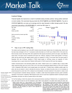
© Copyright 2026