1. Art and Diseño

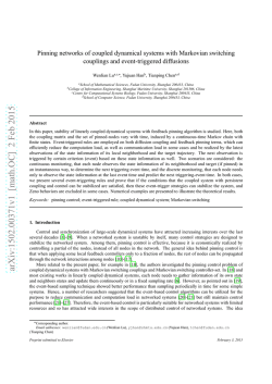
1
A community finding method for weighted dynamic
online social network based on user behavior

Dongming Chen1, Yanlin Dong1, Xinyu Huang1, Haiyan Chen2, Dongqi Wang1*
1. Software College, Northeastern University, Shenyang, 110819, China
2. East China University of Political Science and Law, Shanghai, 200000, China
Abstract—Revealing the structural features of social
networks is vitally important to both scientific research
and practice, and the explosive growth of online social
networks in recent years has brought us dramatic
advances to understand social structures. Here we
proposed a community detection approach based on user
interaction behavior in weighted dynamic online social
networks. We researched interaction behaviors of users in
online social networks and built a directed and
un-weighted network model in terms of the following
relationships between social individuals at the very
beginning. In order to refine the interaction behavior of
users, level one fuzzy comprehensive evaluation model was
employed to describe how closely individuals are
connected to each other. According to this intimate degree
description, weights are tagged to the prior un-weighted
model we built. Secondly, a heuristic community detection
algorithm for dynamic network was provided based on the
improved version of modularity called module density. As
for the heuristic rule, we chose greedy strategy and fed the
algorithms with the update part between two neighboring
time slices’ network model. A parameter β was also set to
evaluate the impacts of individuals’ joining and leaving
actions in directed networks. Experimental results show
that the proposed algorithm can obtain high accuracy and
simultaneously get comparatively lower time complexity
than some typical algorithms. More importantly, our
algorithm needs no priori conditions.
Index Terms — Complex Network, Community Structure,
Modularity, Dynamic Network, Directed and Weighted Network
I.
INTRODUCTION
Research of complex networks has a wide attraction of
scientific research. Some scholars focus on semantic network[1]
which means a form of human knowledge relationships [2][3],
and some other researchers obtain algorithms for community
detection, which is a fundamental problem in network analysis.
Detecting communities is of great importance in sociology,
biology and computer science, disciplines where systems are
often represented as graphs. This problem is so complex that
Dongming Chen (e-mail: [email protected]).
Yanlin Dong (email: [email protected])
Xinyu Huang (email: [email protected])
Haiyan Chen (email: [email protected])
*Dongqi Wang (corresponding author; phone: +86 13624039571; email:
[email protected])
we didn’t find a satisfied solution by far, despite the huge
effort of a large interdisciplinary community of scientists
working on it over the past few years [4].
Traditional methods treat community detection as graph
partitioning and clustering problems. Kernighan-Lin(KL)
algorithm[5] is an early proposed graph partitioning based
method, which uses greedy strategy to optimize the divided
structure according to the edges between communities, the
evaluation function is defined as the number of edges in the
two communities minus the number of edges connecting them.
KL algorithm can divide target network into specific size
subsets, but the number of subsets is needed as a priori. As KL
algorithm, the majority of graph partitioning methods require
too much prior knowledge, and most variants of the graph
partitioning problem are NP-hard. More importantly, the
partitioning results are usually consisted of clusters with
similar size. Taking all these shortcomings into consideration,
graph partitioning algorithms are not fully suitable for
detecting communities in big social networks [6].
Unlike graph partitioning methods, clustering do not need
much prior knowledge, so clustering based methods can be
more effective for community detection. For example,
hierarchical clustering algorithms are known as suitable
approaches to be used to detect communities in social
networks. Social networks naturally have hierarchical
structures, which mean networks with hierarchical structure
may display several levels of grouping of the nodes. Small
clusters are contained within large ones, which are in turn
included in larger ones, and so on [7]. Some clustering
algorithms try to divide a target network naturally into many
parts based on the similarity and intensity of each node, and
these works can be classified into two kinds: aggregation
algorithms and divisive algorithms. For example, the Newman
fast algorithm [8] is a typical aggregation method based on
greedy strategy, mainly focuses on the network with numerous
vertices. Typical divisive algorithm is as method [9], which
treats the network as a huge community, and then divides it
step by step. The GN algorithm proposed by Girvan and
Newman [10] is another example of divisive method. The main
idea is to remove the edges with maximal betweenness [11],
which provides a rule of edge detection for the small
community in the network.
Except for traditional methods, community detection in
weighted, directed or dynamic networks is also widely
discussed separately. Few works took these features together
into consideration, and comparing to the research on
unweighted and undirected networks, no significant
achievements had been made. Most networks in real world can
2
be seen as heterogeneous ones because the nodes have
different characteristics and the relationship between two
nodes usually means different influences to them. In fact,
heterogeneity of nodes can be represented in weighted,
directed network models. On the other hand, dynamic network
analysis had drawn a lot of attentions in the past few years. As
we know, a dynamic community detection method was firstly
proposed by Hopcroft [12], it divided the dynamic network into
several static parts, then obtained the hierarchy clustering
results with the method of cosine similarity. They selected
relatively slightly changed parts from the results as natural
communities, and dynamic network evolution was studied on
the above bases. Chakrabarti [13] tried to analyze dynamic
network via continuous iteration, the concepts called snapshot
quality and history cost were proposed in this work to satisfy
both “clustering results should keep pace with the current
network topology as far as possible” and “the results should
minimize the difference between the clustering process”. In
order to understand the dynamic of social network structure,
Shan build a mathematical model [14], and an incremental
identification method is also proposed, which analyzes the
nodes incrementally rather than just to re-divide all nodes in
the network, to improve actual operation efficiency of the
algorithm. Ning’s work is also a valuable attempt [15], they put
forward the incidence vector concept to present the dynamic
process of the network through incrementally updated
characteristic value system. Chen, Wang and Wei approach a
novel multiobjective algorithm for detecting communities in
dynamic networks, which provides a solution to keep a
balance between accuracy and efficiency [16]. In Yu’s work, a
feasible algorithm for the identification of overlapping
modules in PPI networks is proposed, which detects
communities with more flexibility [17].
As we can see, excellent research works had been done on
community structure detection, however, the existing
algorithms either need too much priori knowledge or not good
enough to handle complex network models. The research on
weighted, directed and dynamic networks may provide us
more ways to understand real networks. And designing fast
and reliable network community detection algorithms will
continue to be the attractive area for us in the future.
On the other hand, with regards to community detection
methods, quality functions are very important, because an
algorithm needs a stopping criterion. Nowadays, the most
commonly known function is called network modularity [18],
which represents one of the first attempts to achieve a first
principle understanding of the clustering problem, and it
embeds in its compact form all essential ingredients and
questions, from the definition of community, to the choice of a
null model, to the expression of the strength of communities
and partitions[4]. Because of this, we are going to employ
modularity in this paper to evaluate the division results and we
take online social network as our target network, a detailed
analysis on the dynamic process of how an online social
network evolves will be shown.
The rest of this paper is organized as follows. Section 2 we
build a weighted social network based on interaction behavior
analysis of online social network. Section 3 gives a
community detection algorithm for dynamic directed weighted
networks. Section 4 compares our method with well-known
algorithms through experiments. Finally, Section 5 makes the
conclusions.
II. SOCIAL NETWORK WEIGHTED METHOD BASED ON USER
INTERACTION BEHAVIOR RESEARCH
When studying network structure, we first focus on the
interactions between individuals and define an approach to
weight the edges to involve more online social network
information into our network model. We assume edge weights
represent the interaction intensity between nodes, which will
reflect both the existing parameters in physical world and
calculating features defined by ourselves. The calculating
features will reveal the underlying characteristics of online
social networks. For a network containing complex social
relationships such as similarity and intimacy, we try to
transform one or more of the interactive attributes to be
weights, to measure the intimacy between users. The method
employed a weight with fuzzy synthetic evaluation model
according to the interaction of followers and the frequency of
interaction over a period of time. The theoretical basis of
weighting method is fuzzy comprehensive evaluation
method[19], which transforms qualitative evaluation to
quantitative evaluation according to the fuzzy membership
degree theory. For short, it is a method to provide an overall
evaluation to objects which are restricted by multiple factors
with fuzzy comprehensive evaluation on multiple factors [20].
In dynamic online social networks, such as Facebook[21]
and microblog [22], the behaviors, for example, 'comment',
'forward', 'like', 'at' can reflect the proximity between users
during a period of time. In our comprehensive evaluation
method, we select the level one comprehensive evaluation
model [23] as the method to measure the relationship. Here we
assume B as the collection of user behaviors:
B = {comment, forward, like, at}
It is crucial to allocate the weight for the above factors.
The weights of the behaviors are confirmed by statistical
methods. The data used in the paper comes from NLP
laboratory of Beijing Institute of Technology which collects
data of Sina microblogs in recent two years [22]. The dataset
contains 1.5 million users and 50 million microblogs. There
are 86,341,256 interaction behaviors, including 21,510,466
'comments', 36,538,478 'like', 23,299,712 'forward' and
4,992,600 'at'. So we can easily figure out the proportion
shown as the following vector A and the member of A is the
proportion of each kind of interactions.
A = (0.2491, 0.4232, 0.2699, 0.0578)
Then we assume a 4  n evaluation matrix R for a single
factor, which is formulated as follows.
r1n 
 r11 r12
r r
r2 n 
Rx   21 22
 r31 r32
r3n 


r4 n 
 r41 r42
Here n represents total number of users x followed, r1n
denotes how many times user x did 'comment' action. r2n
represents how many times user x did 'forward' action, r3n
3
represents how many times user x did 'like' action, r4n denotes
how many times user x did 'at' action, n|x represents user n
was followed by user x. User x’s behavior and connection
relationship with other users are shown in Table 1.
Table 1 Evaluation of user x’s behaviors
Followed
Behaviors
followed_id1
Comment
Forward
Like
At
r11
r12
r13
r14
Matrix R for user x can be calculated as follow:
commentnum(n | x)
(1)
r1n  n
 commentnum(i | x)
forwardednum(n | x)
(2)
n
 forwardednum(i | x)
likenum(n | x)
followed_idn
r21
r22
r23
r24
…
…
…
…
r1n
r2n
r3n
r4n
 0.875
i 1
r3n 
…
We can calculate the evaluation matrix R003 of node 003,
for example, the user did ‘at’ behavior to others for eight
times during a period of time, particularly ‘at’ user 032 for
seven times. So we can get the following data.
atnum(032 | 003)
r4(032|003) 
atnum(009 | 003)  atnum(023| 003)  atnum(032 | 003)
i 1
r2 n 
followed_id2
If we calculate all the data according to the above
(3)
method, we can get the matrix as follows.
n
 likenum(i | x)
i 1
r4 n 
atnum(n | x)
(4)
R003
n
 atnum(i | x)
i 1
Where commentnum(n|x) counts how many times user x
'comment' user n, and forwardednum(n|x) counts how many
times user x 'forward' n’s articles, likenmu(n|x) counts how
many times user x set 'like' tag to user n’s articles and
atnum(n|x) counts how many times user x did 'at' actions to
user n when they post their own articles or comments.
Then we explain the evaluation model with following
Figure 1, which is generated from nodes of sina microblog.
We take user 003 as an example, detailed information can be
discovered in table 2.
0.1667 0.0714 0.1290 0.1250 
  0
0.1429 0.1613
0 
 0.8333 0.7857 0.7097 0.8750 
Finally, we can get the Level I comprehensive evaluation
model B003.
B003  A  R003'
  0.2491 0.4232 0.2699 0.0578  
0
0.8333 
0.1667
 0.0714 0.1429 0.7857 


 0.1290 0.1613 0.7097 


0
0.8750 
 0.1250
  0.1138 0.1040 0.7822 
The result represents the weight value of ‘at’ behavior
from user 003 to the three neighboring users are 0.1138,
0.1040, 0.7822.
III. COMMUNITY PARTITION ALGORITHM FOR DYNAMIC
DIRECTED WEIGHTED NETWORKS
Figure 1 The network of test example.
User_id
003
003
003
Table 2 Statistics of user 003
Comment
Transmit
Attention_id
num
num
009
1
1
025
0
2
032
5
11
Like
num
4
5
22
At
num
1
0
7
This paper proposed an algorithm which needs no priori
conditions, the algorithm firstly set up heuristic rules of the
dynamic changes of the social network based on the basic
nature of community structure, and employed an improved
module density function D combined with weighted network,
to ensure the accuracy of the algorithm [24].
We give some basic definitions which will be used in the
rest part.
For directed weighted network G w  (V , E ,W ) , where V is
the collection of nodes inside Gw, E is the collection of edges
inside Gw, eij  E is an edge from node i to node j, W is the
4
collection of weights of Gw’s edges and
edge
wij is the weight of
eij , we define:
(1) The in-weight and out-weight of nodes in the
network.
The symbol wini represents the sum of all edges weights
i
ending with node i, and wout
denotes the sum of all edges
weights starting with node i.
(2) The inside-edge weight and outside-edge weight in
the community.
Symbol Win (ci ) means the total weight of edges inside a
community, Wout (ci ) discloses the total weight of edges
outside a community, which are shown in formula (5) and
formula (6). An edge inside a community means that both of
the two ends of the edge fall into the community.
(5)
Win(c ) 
w

i
i , jci
Wout (ci ) 

ij
ici , jci
(6)
wij

2
ic1 , jc2
community
c1 and
c 2 where c1 and c 2 are two collections of
disjointed nodes or two communities who have no overlapping
parts between them.
The second function also has two variants as shown in
formula (8),
(8)
L(i, c )  w
i

jci
ij
where i represents a node. Function L counts neighbors of
node i inside community
ci or the increased number of nodes
ci when new node i is added into the
community. Furthermore, Lin (i, ci ) counts the number of
edges from node i to community ci , where Lout (i, ci )
inside community
discloses the number of edges from community
ci to node i.
wd
(4) D (ci ) formulates module density of community
ci , it can be calculated by formula (9).
Win (ci )  Wout (ci )
(9)
2n
Here n is the number of the nodes of the network.
Then we define D wd , which means the increased
D wd  ci  
module density when a node i is added into community
'
ci
to constitute a new community ci , it can be calculated by
formula (10).
D wd  Dtwd
 Dtwd
n
n1
(10)
is an out-degree edge for node i, then the importance of the
node i to the community is 1, otherwise, it is  (0  ＜1) . For
a node of a community, an in-degree edge has more influence
on the community than an out-degree edge. Now we assume
the situation of node i joining into community ci to form a
'
ij
L calculate the sum weights of edges in community
direction is from node j to node i, then only marginal influence
is impressed on the whole community and we can ignore it.
So in the paper, we use a parameter  (0  ＜1) to
represent the weight of in-degree. It means a node i waiting to
join community ci , connected with a directed edge. If the edge
new community ci . As shown in formula (11) and (12),
(3) Function L in directed weighted networks.
Function L is a polymorphism function with two variants
for directed and weighted networks. As shown in formula (7).
(7)
L(c , c ) 
w
1
In order to deal with the affection of direction factor in
the network, we can assume a node i with high out-degree and
low in-degree, while node j is on the contrary. Obviously, if
there is an edge between node i and node j, the direction of the
edge is most possibly from node i to node j. Similarly, if there
is an edge from node i to node j, the module density that of the
community will be greatly influenced, which means that node
i prefers to be a member of community ci . Instead, if the
t
Wint (ci ) calculates Win (ci ) of time t, and Wout
(ci )
calculates Wout (ci ) of time t.
Wint 1 (ci )  Wint (ci )   Ltin (i, ci )  Ltout (i, ci )
t 1
out
W
(11)
(ci )  W (ci )  (   1) L (i, ci ) 
t
out
t
in
(12)
i
(   1) Ltout (i, ci )   ( wini  wout
)
So we can calculate the module density following
formula (13). To make the structure of the new community ci'
more reasonable, we calculate the increased module density
D wd as follows.
W  Win  3 Lin  3Lout   d in  d out
(13)
D wd  out
2n
where n represents the number of nodes of the network.
Formula (13) gives the evaluation rule, which is also the key
of the algorithm in this paper. Most of the algorithms are
based on greedy strategy or approximation algorithm, to
improve the efficiency of calculation.
In our daily life, we can easily find that if a person is my
friend, he or she will most probably be my friend’s friend. So
we prefer to set the node i to be a member of the original
community. Thus, we put forward the principle combining
with heuristic greedy strategy: for any node i in the network,
we prefer to put it into community which contains the most
neighbors of node i. It has two key points: greedy selection
property and optimal substructure.
Our algorithm deals with directed and weighted networks.
However, for a real network, it is almost impossible for the
degree of all nodes to be even. Then, the structure of the
network is an undirected and unlooped graph with a
corresponding matroid. The greedy strategy is one of the
situations of the matroid, so the idea based on module density
with greedy strategy is reasonable.
There are mainly 4 kinds of reasons that will cause the
dynamic variety of real networks. We can conclude them as
follows:
5
(1) Adding a node (V+v): When a new node is joined in
the network, it is likely to connect other edges or not.
(2) Deleting a node (V-v): When a node is deleted, then
all of the edges connected with this node are also removed.
(3) Adding an edge (E+e): Connect two nodes in the
network to produce a new edge.
(4) Deleting an edge (E-e): Remove an edge between two
nodes.
A dynamic community changes its structure in
accordance with the above four situations, and in most cases
the first and the third situations are often occurred, while the
second and the fourth situations are very scarce.
A. Analysis of community structure variations
The four changing situations of a dynamic community
result in the structure of community evolving, too. In the
network we confronted in real life, there are only six cases
when a community structure changes.
(1) Community generation: new nodes are added to a
network dynamically, and these nodes may form a new
community as shown in Figure 2(a).
(2) Community extinction: nodes of a community are
removed gradually, and finally the community disappeared as
shown in Figure 2(b).
(3) Community expansion: the community will expand
when many new nodes or edges are joined as shown in Figure
2(c).
(4) Community decrease: the community will decrease
with the removing of part of nodes or edges and it makes the
community smaller and smaller as shown in Figure 2(d).
(5) Community combination: two communities are
merged into one community dynamically as shown in Figure
2(e).
(6) Community split: a community is split into two or
more communities dynamically as shown in Figure 2(f).
It can be easily proved that the changing results are
among the above six situations.
Null
Null
(a)
(b)
B. Algorithm description
We analyze the four possible dynamic behaviors and design
the algorithm as follows.
(1) Adding a node: When the new node has no connection
with any other nodes, it will be a new independent community.
If the new node has connection with other nodes, we put the
node into the community which can get the highest gain in
module density. The pseudo code of the algorithm is designed
as follows. ( c t denotes the community structure at time t)
Algorithm 1 AddNode
Input: the structure of a community at time t, and a new
node v awaiting to be added
Output: the updated structure at time t+1
// d v is the degree of node v.
If (d v  0) then
Update c t 1  c t {v}
Else
For existing communities, put v into each of them
Do
Calculate D wd
End For
c=get the maximal D wd when node v joins in the
community
Update c t 1  (ct \ c) (c {v})
(2) Deleting a node: If the degree of the removed node is
1, just delete the edge connected to the node, otherwise, delete
all the edges connected to the node and reassign the neighbor
nodes of the deleted node to the community which can achieve
a higher module density. If the connected edges are all within
the community, just keep the neighbor node in the original
community. The pseudo code of deleting a node is given as
follows.
Algorithm 2 DeleteNode
Input: the structure of a community at time t, and the
removed node v
Output: the updated structure at time t+1
k=1;
If (node v’s degree is 1)
c t 1  c t \ c
(c \ v ) {v}
Else
(c)
(e)
(d)
(f)
Figure 2 The six changes of a community
While (Node v’s neighbor is not 0) do
S  {nodes who doesn’t have connections
with nodes outside c }
End while
End if
Put the nodes in S into the considered best community
which has the maximal D wd
Update c t 1
(3) Adding an edge: when the new node i and node j
belong to the same community ( ci  c j ), the new edge from i
to j can enhance the value of function D according to the
definition of module density. So the inside edge will not break
6
up the original community. However, if the two nodes i and j
are not in the same community ( ci  c j ), then the new edge eij
calculate betweenness value for each edge. If the intermediate
value of the removed edge eij is comparatively large, we will
is an outside edge, it will decrease the module density of the
community comparatively. Thus, the new edge may not
change the structure of the community, or make one node in ci
or cj break away from the original community and join another
community so as to obtain higher module density.
When a new edge eij joined into network, we assume
re-divide the community when removing the edge, otherwise,
just keep the original community structure unchanged. The
algorithm is designed as follows:
X  ci ,Y  c j to judge if the new edge will increase the
module density for community Y. The algorithm is designed as
wd
wd
follows, where Dixy
and Dixy
are the gain of module
Algorithm 4 DeleteEdge
Input: the structure of community at time t and the removed
edge eij
Output: the updated structure at time t+1
If ( eij is a single edge) then
c t 1  ( c t \ i{ j, } ) i { } j { }
density when putting node i and j into X and Y.
Else if (the degree of either i or j is 1) then
Algorithm 3 AddEdge
Input: the structure of community at time t, and the new edge
eij.
Output: the updated structure at time t+1
If (node i and node j are new nodes) then
Update c t 1  c t {i, j}
Else if ( ci  c j ) then
wd
If ( Dixy
)
＜0 & D wd
jxy＜0
Update ct 1  ct
Else
wd
wd
Node v = Dixy ＞D jxy？i : j
Move v to the new community
For all neighbors of v
Put it into the best community
which has the maximal ∆Dwd
End for
t 1
Update c
End if
End if
End if
c t 1  ( c t \c (j ) ) i { } c i{ i( ) \ }
Else if (node i and node j don't belong to the same
community) then
ct 1  ct
Else
Int z = Get the betweenness of eij
If (z is the top n biggest betweenness of the
network)
Put other nodes into the considered best
community which holds the maximal D wd
End if
End if
Update c t 1
Then we analyze the time complexity of every step in the
algorithm.
1) Initialization. Initialize N nodes and at most N
communities, which takes the time complexity of O( N ) .
2) Iteration. Iterations are taken place for k times, and to
each iteration, the maximal L(i, ci ) are sought for all of the
N nodes. For node i, the
(4) Deleting an edge: when the nodes i and j of an edge
come from different communities (ci  c j ) , removing the edge
weakens the linkage of intercommunity. Removing an outside
edge makes a higher module density, so it will keep the
original community structure.
When the two nodes(i and j) of the removed edge belong
to the same community (ci  c j ) , if the degree of node i or
node j is 1, then one of the two nodes will be isolated node
after removing the edge. The node will separate from the
original community, and the new separate community will
contain only one node. If the node degree of both i and j are 1,
then two new isolated communities emerged.
When the two nodes (i and j) of the removed edge come
from different communities (ci  c j ) , and the node degree is
different from above, the removing of the outside edge
eij
results a lower module density. Then the original structure
either keeps unchanged or divides into two communities.
Thus, we get the idea from GN algorithm [15], which
regards the community (ci  c j ) as a small network, then
d (i) neighbors are assigned to N
N
communities, so there are at most
 d (i)
times satisfied
i 1
L(i, ci )  0 for each iteration. So it takes time complexity of
N
O(k  d (i )) for searching maximal L(i, ci ) . It must be
i 1
estimated for each iteration to make sure if the constraint
condition is satisfied or not for all of the nodes, which takes
time complexity of O(kN ) .
3) Modification. Algorithm 1 to algorithm 3(described in
section III) are simple linear calculation on given variables,
which takes time complexity O(kN ) , linear calculation on
neighbors of every variable brings complexity
N
O(k  d (i )) .
i 1
7
The total time complexity is
N
community evolution. It also conforms to the objective rule of
‘Rich get Richer’.
N
O( N  k  d (i ) kN  kN  k  d (i )) , which is
i 1
i 1
simplified as O ( kN  k
N
 d (i)) . Assume that the edge
i 1
N
number of the network is E, then
 d (i)  2E , so the final
i 1
In reality, the iteration time will be acceptable for most
networks, so the algorithm will be efficient. Especially, the
more obvious of the community structure will be, the less
iteration time will be needed, and the more efficient will the
algorithm be. However, if the community structure is not clear,
the community detection algorithm will make no sense all the
same.
time complexity is O(kN  kE ) .
From the reckon above, we can get the time complexity
of the algorithm is O(kN  kE ) , N denotes the number of
nodes and E represents edges in the network, and the k is the
number of iteration. Consequently, the value of k is vital in
running the algorithm. From the time complexity proved
above, we can conclude that the consuming time of the
algorithm will decrease with the decline of k value. So, the
smaller the k value becomes and the faster the algorithm runs.
According to the Heuristic principles of basic property in
community structure, the algorithm will need to detect a
community from the node with more neighbor nodes as
possible. Obviously, the more nodes a community contains,
the more suitable for algorithm to detecting, which enable the
main community become greater during the dynamic
Table 3

dataset size
IV. EXPERIMENT AND ANALYSIS
In this section, we carry out the experiments by using
Sina microblog dataset with 5,000 users. And we establish
four networks with 100, 500, 1000 and 5000 nodes
respectively. To show the results conveniently, we choose
some representative nodes to build a small network. Then we
compare the efforts with other algorithms.
Firstly, to confirm the value of  , we do the experiment
with different network scale(dataset size). When the
experiments end, we choose the value of  when the
community obtains the maximum value of module density.
The results are shown in Table 3.
Relation between  and module density
0.40
0.45
0.50
0.55
0.60
0.65
0.70
0.75
0.80
S100
0.399
0.420
0.442
0.459
0.467
0.471
0.456
0.433
0.384
S500
0.435
0.473
0.494
0.509
0.522
0.519
0.498
0.492
0.478
S1000
0.511
0.537
0.554
0.568
0.577
0.585
0.575
0.560
0.542
S5000
0.553
0.592
0.627
0.658
0.683
0.697
0.680
0.657
0.621
From Table 3, we can conclude that in most cases when
the value of  is 0.65, the module density will reach the
maximal value. Thus, we choose the approximate value of
  0.65 for the rest experiments.
Comparing with extremal optimization algorithm [25] and
improved CNM algorithm [26], we do experiments to get the
time overhead and the module density. The comparison results
are listed in Table 4 and Table 5.
Table 4 Time Overhead comparison of different algorithms
dataset size
S100
S500
S1000
algorithms
Our algorithm
Extremal optimization
Improved CNM algorithm
algorithms
0.285
0.317
0.279
1.962
2.231
2.195
7.450
7.983
7.964
Table 5 Modularity comparison of different algorithms
dataset size
S100
S500
S1000
Our algorithm
Extremal optimization
Improved CNM algorithm
0.369
0.362
0.347
From Table 4 and Table 5, we can conclude that the
algorithm in this paper outperforms in time consuming
compared with extreme optimization and improved CNM
algorithm as an increasing in network scale [26].
0.433
0.405
0.398
0.527
0.485
0.451
S5000
105.317
132.250
125.725
S5000
0.573
0.510
0.494
To demonstrate the high quality of the divided results,
we can evaluate the module density of the algorithms. Figure 3
shows the changing tendency of module density when network
scale increases, which discloses the larger of the network scale,
8
the bigger of the module density will be. Module density
reflects the divisive quality of network, so the proposed
algorithm is suitable for large scale network.
Module Density
Module Density
0.8
0.6
0.4
0.2
0
0
5
10
time (s) 15
value of module density S100
value of module density S500
value of module density S1000
value of module density S5000
Figure 3
Changing Tendency of Module Density
The above experiments have presented the results in
static networks. So we randomly add four behaviors of
dynamic network variations (described in section 3) to
compare with the other algorithms. The adjustment of the
community is based on increments of the network and it is
locally conducted, even in the most complex situations, the
time expenses of the algorithm can be neglected, and the
results are shown in Figure 4.
for online social networks are provided in this paper, which
are suitable for dynamic social network modeling and
community detecting, considering with the characteristics of
the social network and the shortage of the most current
community partition algorithm. According to the real-time and
dynamic characteristics of the social network, we first
weighted the network edge based on the user's behaviors, then
combined the following methods to design a new community
partition algorithm: the strategy of greedy heuristic rules,
improve module density function D in terms of the
characteristics of the weighted and directed network, which is
employed to derive the standard measure function for
estimating community detection and dynamic rules in real
social network. The algorithm can obtain very high accuracy
and low time complexity without any priori condition.
Moreover, the complexity only depends on the number of
iterations, namely the clarity of the community structure of
network, and regardless of the scale of the network, so it is
suitable for dynamic and large scale network analysis.
ACKNOWLEDGEMENT
This work is supported by the Central Universities
Fundamental Research funding of China under Grant No.
N120317003.
REFERENCES
[1]
Modularity
0.4
0.35
0.3
0.25
0.2
0.15
0.1
0.05
0
Modularity
[2]
[3]
[4]
0
Figure 4
5
10
algorithm in this paper
extremal optimization
improved CNM algorithm
15
[5]
time (s)
[6]
Changing Tendency of Modularity
We can conclude that during the process of changes, all
the module density values of the three algorithms have a bit
fluctuation, but just in a small range relatively(from 0.26 to
0.37), and the algorithm in this paper always maintains the
highest module density value after a certain time (time = 4.5s)
in dynamic network as shown in Figure 4.
In brief, the algorithm in this paper can achieve better
results compared with the extremal optimization and improved
CNM algorithm.
V. CONCLUSIONS
A weighted approach based on user interaction behavior
and module density based communities detection algorithm
[7]
[8]
[9]
[10]
[11]
[12]
[13]
[14]
Luo X, Xu Z, Yu J, et al. Building association link network for semantic
link on web resources[J]. Automation Science and Engineering, IEEE
Transactions on, 2011, 8(3): 482-494.
Xu Z, Wei X, Luo X, et al. Knowle: a semantic link network based
system for organizing large scale online news events[J]. Future
Generation Computer Systems, 2014.
Xu Z, Luo X, Wang L. Incremental building association link network[J].
International Journal of Computer Systems Science & Engineering, 2011,
26(3): 153-162.
Fortunato S. Community detection in graphs[J]. Physics Reports, 2010,
486(3): 75-174.
Kernighan B.W, Lin S. An efficient heuristic procedure for partitioning
graphs [J]. Bell System Technical Journal, 1970, 49: 291-307.
Bhattacharyya S, Bickel P J. Community detection in networks using
graph distance[J]. arXiv preprint arXiv:1401.3915, 2014.
Malliaros F D, Vazirgiannis M. Clustering and community detection in
directed networks: A survey[J]. Physics Reports, 2013, 533(4): 95-142.
Newman M.E.J. Fast algorithm for detecting community structure in
networks [J]. Phys Rev E, 2004, 69(6): 066133.
Albert R, Barabasi A.L. Statistical mechanics of complex networks [J].
Review of ModernPhysics, 2002, 74: 47–91.
Girvan M, Newman M E J. Community structure in social and biological
networks[J]. Proceedings of the National Academy of Sciences, 2002,
99(12): 7821-7826.
Newman M.E.J. Analysis of weighted networks[J]. Physical Review E
(Statistical, Nonlinear, and Soft Matter Physics), 2004, 705 Pt 2:.
Hopcroft John, Khan Omar, Kulis Brian, et al. Tracking evolving
community in large linked networks [J]. PNAS. 2004, 101(11):
5249-5253.
Chakrabarti D, Kumar R, Tomkins A. Proceedings of the 12th ACM
SIGKDD International Conference on Knowledge Discovery and Data
Mining [J]. ACM, New York, USA. 2006: 554-560.
Shanbo, Jiang Shouxu, Zhang Genshuo. IC: Dynamic social network
community structure of incremental recognition algorithm [J]. Journal of
Software. 2009, 20(Supplement): 184-192.
9
[15] Ning Huazhong, Xu Wei, Chi Yun, et al. Incremental spectral clustering
with application to monitoring of evolving blog communities [J]. SIAM
Internation Conference on Data Mining, 2007.
[16] Chen G, Wang Y, Wei J. A new multiobjective evolutionary algorithm
for community detection in dynamic complex networks[J].
Mathematical problems in engineering, 2013.
[17] Yu Q, Li G H, Huang J F. Mofinder: A novel algorithm for detecting
overlapping modules from protein-protein interaction network[J].
BioMed Research International, 2012.
[18] Newman M E J. Modularity and community structure in networks[J].
Proceedings of the National Academy of Sciences, 2006, 103(23):
8577-8582.
[19] Barabasi A.L, Bonabeau E. Scale-Free Networks [J]. Scientific
American, 2003, 288(1): 60-69．
[20] Guo Y. Comprehensive evaluation theory and method[J]. Press of
Science and Technology, Beijing, 2002: 41-46.
[21] Facebook: https://www.facebook.com/
[22] Sina microblog: http://us.weibo.com/gb
[23] F0RTUNATO S, BARTHELEMY M. Resolution 1imit in community
detection [J]. PPNAS, 2007, 104(1): 36-41.
[24] Zhenping Li, Shihua Zhang, Rui-Sheng Wang. Quantitative function for
community detection [J]. Physical Review E, 2008, 77: 036109.
[25] Duch J, Arenas A. Community detection in complex networks using
extremal optimization[J]. Physical review E, 2005, 72(2): 027104.
[26] Wakita K, Tsurumi T. Finding community structure in mega-scale social
networks:[extended abstract][C]//Proceedings of the 16th international
conference on World Wide Web. ACM, 2007: 1275-1276.
The authors declare that there is no conflict of interests
regarding the publication of this article.