1. Art and Diseño

Designing and Evaluating an Interpretable Predictive
Modeling Technique for Business Processes
Dominic Breuker1, Patrick Delfmann1, Martin Matzner1 and
Jörg Becker1
1
Department for Information Systems, Leonardo-Campus 3,
48149 Muenster, Germany
{breuker, delfmann, matzner, becker}@ercis.com
Abstract. Process mining is a field traditionally concerned with retrospective
analysis of event logs, yet interest in applying it online to running process
instances is increasing. In this paper, we design a predictive modeling technique
that can be used to quantify probabilities of how a running process instance will
behave based on the events that have been observed so far. To this end, we study
the field of grammatical inference and identify suitable probabilistic modeling
techniques for event log data. After tailoring one of these techniques to the
domain of business process management, we derive a learning algorithm. By
combining our predictive model with an established process discovery technique,
we are able to visualize the significant parts of predictive models in form of Petri
nets. A preliminary evaluation demonstrates the effectiveness of our approach.
Keywords: Data mining, process mining, grammatical inference, predictive
modeling
1 Motivation
In recent years, business analytics has emerged as one of the hottest topics in both
research and practice. With stories praising the opportunities of data analysis being
omnipresent, it is not surprising that scholars from diverse fields explore how data can
be exploited to improve business understanding and decision making. In business
process management (BPM), a research discipline called process mining has emerged
that deals with analyzing historical data about instances of business processes [1]. The
data usually comes in form of event logs, which are collections of sequences of events
that have been collected while executing a business process. Events are of different
types. The type describes the nature of an event. For instance, an event could represent
an activity that was performed or a decision that was made.
Traditionally, process mining has been used mainly for retrospective analysis. The
primary task of many process mining techniques is to discover the underlying process
given an event log, with the goal of providing analysts with an objective view on an
organization’s collective behavior [2]. Further analyses can follow. One could verify
that a process conforms to a given specification or improve the process based on the
discovered insights [1].
In recent times, interest has been expressed into applying process mining no only ex
post but also in an online setting. The idea is to apply insights gained from event logs
to currently running process instances. The goals could be to predict properties of
interest or recommend good decisions [3]. Techniques have been designed to predict
the time at which a process instance will be completed [4] or to recommend performers
for tasks such that performance is maximized [5].
In this paper, we consider a similar prediction problem. Interpreting events of an
event log as outcomes of decisions, our goal is to build a predictive analytics model
that accounts for the sequential nature of decision making in business processes.
Provided with a partial sequence of events from an unfinished process instance, the
model’s task is quantifying the likelihood of the instance ending with certain future
sequences. The model should be trained solemnly by means of event log data.
Such a predictive model could be useful in variety of situations. For instance, early
warning systems could be built. Decision makers could be provided with a list of
running process instances in which undesirable events will likely be observed in the
future. A predictive model could also be used to estimate how many running instances
will require a certain resource, again to warn decision makers if capacities will be
exceeded. Moreover, anomaly detection approaches could be built to identify highly
unlikely process instances. They could help pointing business analysts to unusual
instances. It is also conceivable to use a predictive model to support other process
mining endeavors, for instance by imputing missing values in incomplete event logs.
The first step in constructing a predictive modeling approach is defining a suitable
representation of the data and the model structure. To find one, we tap into research
from the field of grammatical inference, which is the study of learning structure from
discrete sequential data [6], often by fitting probabilistic models [7]. After identifying
a suitable model, we also discuss how to fit the model to data. Again, we draw on
grammatical inference to identify a suitable technique. Subsequently, we adapt the
probabilistic model to the BPM domain. As a consequence, we have to adapt the fitting
technique too. By applying the predictive modeling approach to real-world event logs,
we illustrate how it can be used and demonstrate its effectiveness.
The primary goal of our modifications is to define the probabilistic model such that
its structure most closely resembles the structure of business processes. An advantage
of that is that models with appropriate structure typically perform better when used in
predictive analytics. The other goal is to keep the model interpretable. Whenever nontechnical stakeholders are involved in predictive analytics endeavors, interpretability
can be crucial to get them on board. For this reason, interpretable models may be
preferred even if they perform worse than their black box counterparts [8]. By
combining a technique from process mining [9] with our predictive modeling approach,
we are able to visualize a predictive model’s structure in form of process models. This
puts domain experts in the position to judge the quality of a predictive model.
The remainder of this paper is structured as follows. In section 2, we discuss
probabilistic models and fitting techniques used in grammatical inference. Section 3 is
devoted to the BPM-specific modifications we designed. In section 4, we describe how
process mining can be applied to create visualizations. The evaluation of our approach
is documented in section 5. In section 6, we conclude and give an outlook to future
research.
2 Grammatical inference
2.1 Probabilistic models of discrete sequential data
The inductive learning problem tackled in grammatical inference [10] starts with a data
(𝑐)
(𝑐)
set 𝑋 = {𝑥 (1) , … , 𝑥 (𝐶) } with 𝐶 strings. Each string 𝑥 (𝑐) is a sequence (𝑥1 , … , 𝑥𝑡𝑐 ) of
symbols 𝑡𝑐 , all of which are part of an alphabet: 𝑥𝑡 ∈ {1, … , 𝐸}. The number of different
symbols shall be denoted 𝐸. When interpreting the data as an event log with 𝐶 process
instances, each of which consists of a sequence of events which, in turn, a part of the
alphabet of event types, grammatical inference can be readily applied to event log data.
The task is to learn a formal representation of the language from which the sample
strings in the data originate. These representations are either automata or grammars [6].
Instead of building automata and grammars that decide if strings belong to a language,
it is often more useful to build probabilistic versions of these representations [10]. This
allows further analyses such as finding the most probable string or predicting how likely
certain symbols are given partial strings.
Since it is our goal to apply grammatical inference to the domain of BPM, we focus
our discussion on automata. Automata consist of states and transitions between these
states. By contrast, grammars consist of production rules that do not directly encode
any states. A state-based representation appears most natural as modeling techniques
used in BPM follow similar principles. Most importantly, explicit state modeling is one
of the reasons for the popularity of Petri nets [11].
A‘
π
A
π
Z0
Z1
Z2
...
Z0
Z1
Z2
...
X0
X1
X2
...
X0
X1
X2
...
B
(a)
B
(b)
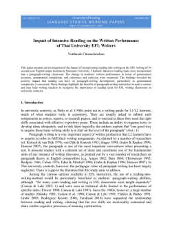
Fig. 1. Directed graphical models of an HMM (a) and a PFA (b). Circles represent
random variables and are shaded grey if observations will be available. Directed arcs
encode dependencies of random variables among each other. Conversely, missing arcs
imply conditional independencies. Parameters are represented as solid black dots and
are connected via dashed, undirected arcs to the random variables to whose
distributions they belong [12]
There are many different variants of automata studied in the literature. Two of them
are most popular [7]. One is the Hidden Markov Model (HMM), the other is the
Probabilistic Finite Automaton (PFA). HMMs [13] are generative models of string
distributions. They use an unobserved state space to explain how the strings have been
generated. To that end, discrete time steps are defined and the model’s state evolves in
time. At each step, the HMM is in one state and emits a symbol. The probability of
emitting a symbol depends only on the current state. Then, the HMM transitions to
another state which it is in in the next time step. The transition probability also depends
only on the current step’s state. Fig. 1 (a) illustrates the HMM.
Reflecting the HMM’s model structure against the backdrop of the BPM domain
unveils a problem. The process is driven mainly by the HMM’s states and the
transitions between them. The symbols however do not influence these transitions. In a
typical business process though, we would expect the next state to depend on the event
we have just observed. Consider the example of Petri nets, in which the state after firing
a transition clearly depends on which transition is chosen. As the HMM assumes
independence, we discard it is a probabilistic model for business processes.
This motivates considering the PFA [14]. We illustrated another graphical model in
Fig. 1 (b). It is similar to that of the HMM, but with an additional arc from each symbol
to the following state. Effectively, this arc removes the problematic assumption of
independence. This model can now serve as the probabilistic equivalent of automata as
applied in the BPM domain.
2.2 Learning techniques
Approaches to learn probabilistic automata can be categorized broadly into three
classes [7]. Those from the first class start with a very complex structure and iteratively
merge states until the structure is simple enough. Approaches from the second class
assume a standard structure and optimize parameters such that the likelihood of the data
is maximal. The third class of approaches consists of sampling methods that rely not on
estimating any model but on averaging over many possible models.
In a recent grammatical inference competition, different state-of-the-art learning
approaches have been benchmarked against each other on a large collection of data sets
[15]. The winning team [16] has designed a collapsed Gibbs sampler to estimate string
probabilities, i.e., they applied a method from the third class. Second best scored a team
[17] that used maximum likelihood (ML) estimation, i.e., the standard technique from
the second class. Methods from the first class have also been applied, yet they scored
worse than the others.
These results may indicate that sampling methods are the most promising learning
techniques. However, they have an important drawback. While approaches from other
categories deliver explicit representations of the analyzed processes along with
interpretable parameters, the Gibbs sampling techniques draws randomly many such
representations and averages over them when predicting. As a result, there is no way to
compactly visualize the predictive model anymore. However, one of our design goals
is to avoid creating a black box learning method. Hence, we design our approach not
based on sampling techniques but instead based on parameter optimization, i.e., a
technique from the second class.
3 PFA learning with event logs
3.1 Adapting the PFA model
In this section, we define two modifications of the PFA model of section 2.1. The first
addresses the problem of overfitting to small data sets. It is well-known that an ML
estimator is at danger of delivering results that fit well to training data but perform
badly on new data [18]. For process data, overfitting can be a severe problem. Process
miners consider incompleteness of data as one of the major challenges their discipline
has to tackle [19]. Consequently, we have to take precautions.
100x Heads
1x Heads
start
0
1.0
1.0
(a)
kill
MAP
estimate
...
end
1
ML
estimate
1
1.0
H
0
T
1
0
H
T
H
T
1
H
0
T
(b)
Fig. 2. Illustration of the modifications to the PFA model. (a) illustrates the
predefined start and end states. (b) illustrates the effect of Bayesian regularization.
For our probabilistic model, we address this problem with Bayesian regularization
[20]. This technique is best illustrated with the simple example of tossing a two-sided
coin (cf. Fig. 2 (b) for the following explanation). Consider two data sets. In the first,
heads was observed once, in the second, heads was observed 100 times. If the goal is
to estimate 𝑝, the probability of heads, then for both data sets, the ML estimate will be
𝑝 = 1. In the first scenario, we overfit to the small data set. This can be avoided by
smoothing the estimates with artificial observations. In the example of Fig. 2 (b), we
can add one artificial observation of both heads and tails, which would deliver an
estimate of 𝑝 = 2/3 in the first scenario and 𝑝 = 101/102 in the second. This is
achieved by interpreting 𝑝 not as a parameter but also as a random variable with a
distribution. When using the beta distribution in this example, the beta distribution’s
parameters can be used to specify the artificial observations [21]. Estimating 𝑝 in such
a setting is called Maximum a posteriori (MAP) estimation.
We can move to MAP estimation in our PFA model by treating the parameters as
random variables and by defining their distributions to be Dirichlet distributions, which
are conjugate priors for the discrete distributions used to define the other variables [21].
The parameters of the Dirichlet distributions can be interpreted as the artificial
observations we want to add when estimating parameters of discrete distributions. See
Fig. 3. (a) for the graphical model corresponding to the regularized PFA and Fig. 3. (b)
for a formal definition of the model.
R
ρ
S
A
Z0
Z1
Z2
...
X0
X1
X2
...
π
B
(a)
(b)
Fig. 3. (a) shows the graphical model of the modified PFA. (b) shows the definition
of the model’s discrete and Dirichlet distributions.
The second modification is motivated by the notion of workflows nets, a special
class of Petri nets well known in the BPM domain [11]. Workflow nets have designated
start and end places (the source and sink) since well-designed process models should
clearly show where the process starts and ends. We impose the same constraints on the
PFA model.
To implement these constraints, we define a special starting state by keeping the
vector 𝜋 fixed at a value that allows the process to start only in that state. In the same
way, a special ending state is defined in which only a designated termination event
“kill” can be emitted. Also, the process is forced to stay in that state. Kill shall be an
event that can only be emitted in the ending state. All other states have zero probability
of emitting it. When processing he event log, the Kill must be appended to the end of
each process instance. Fig. 2 (a) illustrates the structural assumptions described above.
They can all be enforced by keeping the corresponding parameters fixed at suitable
values while executing the learning algorithm.
3.2 Learning algorithm
MAP estimation aims at maximizing the posterior probability 𝑃(𝜃|𝑋). 𝜃 denotes all
parameters that must be estimated. This optimization can be implemented by
optimizing the following expression: 𝜃 ∗ = arg max[𝑃(𝑋|𝜃)𝑃(𝜃)] [22]. Direct
𝜃
optimization is computationally intractable in presence of unobserved variables such as
our state variables. A solution is to apply the expectation maximization (EM) procedure
[23]. Starting with (random) initial parameters, it iterates between computing the
expectation of the hidden state variables 𝑍 with respect to current parameters 𝜃 𝑜𝑙𝑑 (i.e.,
𝔼𝑍|𝑋,𝜃𝑜𝑙𝑑 ln 𝑃(𝑋, 𝑍|𝜃)) and deriving updated parameters 𝜃 𝑛𝑒𝑤 by optimizing them with
respect to this expectation over states (i.e., 𝜃 𝑛𝑒𝑤 = arg max[𝔼𝑍|𝑋,𝜃𝑜𝑙𝑑 ln 𝑃(𝑋, 𝑍|𝜃) +
𝜃
ln 𝑃(𝜃)]). The algorithm stops once a local optimum is reached [24]. This optimum
depends on the initial parameters, which is why it is advisable to run EM multiple times
with different initial values to avoid bad local optima [25].
To apply EM to our probabilistic model, we must implement the four steps initial
parameter definition, E-step, M-step, and the check for convergence. Our
implementation generates initial parameters randomly, with the exception that we
enforce a starting and ending state as described in section 3.1. The corresponding
parameters are fixed at 0 and 1 respectively. Convergence is also determined in the
standard way, i.e., by defining a threshold and stopping the algorithm if the likelihood
of the data does not improve enough after updating parameters.
To implement the E-step and M-step, we start with 𝜃 𝑛𝑒𝑤 =
arg max[𝔼𝑍|𝑋,𝜃𝑜𝑙𝑑 ln 𝑃(𝑋, 𝑍|𝜃) + ln 𝑃(𝜃)] and use Lagrangian multipliers to derive
𝜃
updating equations. These updating equations can be found in equations 1-3. They all
consist of a data-term, which is the contribution of the event log data, and a prior-term,
which is the contribution of the corresponding Dirichlet distribution. In each M-step,
these updating equations are used to compute updated parameter values.
𝑑𝑎𝑡𝑎𝑘 + 𝑝𝑟𝑖𝑜𝑟𝑘
∑𝐾
𝑗=1(𝑑𝑎𝑡𝑎𝑘 + 𝑝𝑟𝑖𝑜𝑟𝑘 )
(1)
𝑏𝑘𝑒 =
𝑑𝑎𝑡𝑎𝑘𝑒 +
𝐸
∑𝑒=1(𝑑𝑎𝑡𝑎𝑘𝑒
𝑝𝑟𝑖𝑜𝑟𝑘𝑒
+ 𝑝𝑟𝑖𝑜𝑟𝑘𝑒 )
(2)
𝑎𝑘𝑒𝑗 =
𝑑𝑎𝑡𝑎𝑘𝑒𝑗 +
𝐾
∑𝑗=1(𝑑𝑎𝑡𝑎𝑘𝑒𝑗
𝑝𝑟𝑖𝑜𝑟𝑘𝑒𝑗
𝜋𝑘 =
+ 𝑝𝑟𝑖𝑜𝑟𝑘𝑒𝑗 )
(3)
In each E-step, the data-terms are computed (the prior-terms are fixed and require
no computations). All terms are shown in equations 4-9. Within these equations,
(𝑐)
𝑇𝑒 denotes the set of points in time at which an event of type 𝑒 is observed in instance
(𝑐)
𝑥 . 𝑇 (𝑐) denotes all points in time regardless of the event types. All data-terms consist
of sums over marginal distributions over the state variables. For our probabilistic
model, they can be computed efficiently with a standard procedure called belief
propagation [26], which we have implemented in our E-step.
𝐶
(𝑐)
𝑑𝑎𝑡𝑎𝑘 =
∑ 𝑃(𝑍0 = 𝑘|𝑋 (𝑐) , 𝜃 𝑜𝑙𝑑 )
𝑝𝑟𝑖𝑜𝑟𝑘 =
𝜌𝑘 − 1
(4)
𝑐=1
(5)
𝐶
𝑑𝑎𝑡𝑎𝑘𝑒 =
(𝑐)
∑ ∑ 𝑃(𝑍𝑡
= 𝑘|𝑋 (𝑐) , 𝜃 𝑜𝑙𝑑 )
(6)
𝑐=1 𝑡∈𝑇 (𝑐)
𝑒
𝑝𝑟𝑖𝑜𝑟𝑘𝑒 =
𝑠𝑘𝑒 − 1
(7)
𝐶
𝑑𝑎𝑡𝑎𝑘𝑒𝑗 =
∑
∑
(𝑐)
(𝑐)
𝑃(𝑍𝑡−1 = 𝑘, 𝑍𝑡
= 𝑗|𝑋 (𝑐) , 𝜃 𝑜𝑙𝑑 )
(8)
𝑐=1 𝑡∈𝑇 (𝑐) ,𝑡≠0
𝑒
𝑝𝑟𝑖𝑜𝑟𝑘𝑒𝑗 =
𝑟𝑘𝑒𝑗 − 1
(9)
3.3 Model selection
The learning algorithm described in the previous section must be provided with some
input parameters. To define the dimensions of the probabilistic model, the number of
event types 𝐸 and the number of states 𝐾 must be given. The former is known, but the
latter must be chosen arbitrarily. Hence, we use grid search to determine appropriate
values for 𝐾. The same is necessary for 𝜌, 𝑆, and 𝑅, the parameters of the Dirichlet
distributions. As we do not want to bias the model towards certain decisions, we use
symmetric Dirichlet priors. However, the strength of these parameters must still be
chosen arbitrarily, which again requires grid search.
In grid search, a range of possible values is defined for all parameters not directly
optimized by EM. For each combination of values, EM is applied. The trained models
from all these runs are subsequently compared to choose one that is best. Different
criteria can be applied in this comparison. One solution is assigning a score based on
likelihood penalized by the number of parameters, which favors small models. The
Akaike Information Criterion (AIC) [27] is a popular criterion of this kind. One
disadvantage of the AIC applied to probabilistic models of processes is that we would
expect the models to be sparse, i.e., we expect that most transitions have very low
probability. Hence, we also consider a less drastic criterion which we call the Heuristic
Information Criterion (HIC). It penalizes the likelihood by the number of parameters
exceeding a given threshold.
A different solution is to split the event log into a training set used for learning and
a validation set used to score generalization performance. According to this criterion,
the model performing best on the validation set is chosen.
4 Model structure visualization and analysis
Since we carefully designed the probabilistic model to be interpretable, it is possible to
derive meaningful visualizations from a learned model. Using the parameters, we could
directly draw an automaton with 𝐾 states and 𝐸𝐾 2 transitions, i.e., a full graph. For all
but the smallest examples though, the visualization would not be useful as it would be
too complex. However, we can prune the automaton such that only sufficiently probable
transitions are kept. For each transition, we delete it if its probability 𝑏𝑘𝑒 𝑎𝑘𝑒𝑗 is smaller
than a given threshold. As there are 𝐾𝐸 transitions going out of each state, each
transition would have a probability of 1/(𝐾𝐸) if all were equally probable. If they are
not, then the probability mass will focus at the probable transitions, while probabilities
of the improbable transitions will fall below this value. Hence, we define the pruning
ratio 𝑝𝑟𝑢𝑛𝑒 relative to 1/(𝐾𝐸). Thresholds are defined as 1/(𝑝𝑟𝑢𝑛𝑒 ⋅ 𝐾𝐸), such that
a pruning ratio of 𝑝𝑟𝑢𝑛𝑒 = 1.5 means throwing away all transitions being 1.5 times as
unlikely as if all transitions had probability 1/(𝐾𝐸).
As we effectively construct an automaton from an event log with this procedure, our
technique has delivered not only a prediction approach but can also be used as a process
discovery algorithm. To this end, we combine it with a technique that was used in the
region miner algorithm [9]. In this algorithm, an automaton is constructed and then
transformed into a Petri net using a tool called Petrify [28]. Hence, we can also apply
Petrify to transform our pruned automata to Petri nets. We have implemented the entire
approach as a process mining plugin for ProM1.
While discovering processes with our approach might have merits in itself, our
primary motivation is to provide non-technical audiences with a visualization of a
predictive model. If a stakeholder must be convinced that a certain predictive model
should be implemented in his organization, the visualization approach could be used to
build trust. Stakeholders can see in form of familiar process modeling notations what
the most probable paths through the predictive model are.
5 Evaluation
Experimental setup
To evaluate our approach as a predictive modeling technique, we apply it to a real-life
event log from the business process intelligence challenge in 2012 [29]. It originates
from a Dutch financial institute and contains about 262,000 events in 13,084 process
instances. There are three subprocesses (called P_W, P_A, and P_O) and each event is
uniquely assigned to one subprocess. Apart from the complete event log, we generated
three additional event logs by splitting the complete log into these subprocesses. Each
of the four event logs is split into a training set (50%), a validation set (25%) and a test
set (25%). The training set is used to run EM, the validation set is used during model
selection, and the test set is used to assess final performance.
The EM algorithm was configured in the following way. Convergence was achieved
when the log-likelihood increased less than 0.001 after the M-step. As a grid for 𝐾, we
used [2,4,8,10,12,14,16,18,20,30,40]. The grid for the Dirichlet distributions’ strength
was defined relative to the sizes of the event logs. The overall number of artificial
observations, distributed symmetrically over all Dirichlet distributions, was optimized
over the grid [0.0, 0.1, 0.2, 0.3, 0.4, 0.5, 0.75] and is expressed as a fraction of the total
number of events in the logs. To compare different models in grid search, we separately
tried all three methods described in section 3.3, with the HIC applied with a threshold
of 0.05.
One measure to estimate the quality is H, the cross entropy (as estimated w.r.t. the
test set). We also consider a number of different prediction problems that could occur
in practice. The most straightforward one is predicting what the next symbol will be.
We report the average accuracy of our predictors. Accuracy is the fraction of
predictions in which the correct event has been predicted. The other prediction problem
is concerned with specific types of events. After selecting an event type, the task is to
predict whether or not the next event will be of this type. We measured the sensitivies
(true positives) and specitivities (true negatives) for each predictor applied to the
problem of deciding this for each event.
Note that our approach is not restricted to predicting the next event. Evaluating the
distribution over an event arbitrarily far in the future is also feasible. However, our
evaluation focusses on predicting the next event only.
1
http://goo.gl/FqzJwp
Results
In Table 1, we list the results for all four event logs (P_W, P_A, P_O, and P_Complete).
For each, we report performance statistics for the three different model selection criteria
(EM_HIC, EM_AIC, and EM_Val). The sensitivities and specificities have been
averaged over all symbols to keep the table compact.
A first observation is that accuracies do not rise up close to 1. However, accuracies
that high cannot be expected, since there is inherent uncertainty in the decisions made
in business processes. Thus, predicting the next event correctly must fail in some cases.
Predicting events completely at random would deliver the correct event with probability
1/𝐸. For the three events logs, accuracies of random prediction would be below 0.10.
Hence, our approach is significantly better than random guessing.
As for comparing the model selection criteria, the results demonstrate that using the
validation set to assess performance delivered solid results if measured by cross
entropy. For this metric, the validation set always delivered the best model, i.e., the one
with the smallest cross entropy.
This is changing though if we turn to the actual prediction problems. The HIC
performed best on P_Complete and P_A, yet bad on P_W, for which the AIC worked
better. For event log P_O, all three methods deliver nearly the same performance.
Hence, our preliminary results indicate that no model selection criterion can generally
outperform the others.
Table 1. Accuracy, average sensitivity and average specitivity for different predictive models.
Event log
P_W
P_A
P_O
P_Complete
Predictor
EM_HIC
EM_AIC
EM_Val
EM_HIC
EM_AIC
EM_Val
EM_HIC
EM_AIC
EM_Val
EM_HIC
EM_AIC
EM_Val
Accuracy
0.685
0.719
0.718
0.801
0.769
0.796
0.809
0.811
0.811
0.735
0.694
0.700
Ø Sensitivity
0.558
0.578
0.582
0.723
0.658
0.720
0.646
0.647
0.647
0.508
0.460
0.437
Ø Specitivity
0.950
0.955
0.955
0.980
0.977
0.980
0.973
0.973
0.973
0.988
0.986
0.986
H
12.810
11.183
10.385
3.093
3.393
3.014
4.588
4.513
4.513
17.273
17.726
16.078
In Fig. 4, an exemplary Petri net visualization is shown. It has been generated from
a predictor for event log P_A, chosen by the HIC. An analyst could double-check this
visualization with his domain knowledge. Alternatively, he could apply other process
discovery techniques to verify that the predictive model is indeed a good model for the
event log. Comparing this Petri net with results found during the challenge, we can see
that the visualization of the predictor is almost identical to what has been discovered
with other methods [30]. Hence, this visual comparison with other findings delivers
further evidence for the appropriateness of the predictive model.
Fig. 4. Petri net visualization of predictor fitted with the HIC criterion, generated
with the ProM plugin and a pruning ratio of 1.5.
6 Conclusion and Outlook
In this paper, we presented an approach to apply predictive modeling to event log data.
We discussed different representations used in the literature of grammatical inference
to model formal languages probabilistically. Against the backdrop of the BPM domain,
we identified probabilistic versions of finite automata to be most appropriate. We also
identified suitable learning techniques to fit these models to data. Starting with this
theoretical background, we modified the probabilistic model to tailor it to the problem
at hand. Subsequently, we derived an EM optimization algorithm, defined a grid search
procedure to also optimize its inputs, and tested the approach on real-world event logs.
Our preliminary results demonstrate the applicability of the approach. With the ProM
plugin, in which we combined the predictive approach with ProM’s Petri net synthesis
capabilities, we provide a readily applicable process discovery tool.
In future research, we plan to conduct more extensive evaluations. In particular, we
will systematically compare our model selection criteria to identify which work best
under which circumstances. Adding experiments with synthetic data may also allow us
to thoroughly investigate the performance of the predictive approach with respect to a
known gold standard. For the real-life event log we used in the preliminary evaluation,
the “true” probabilities are unknown, so that we cannot quantify the quality of the
predictors generated with our approach in absolute terms.
References
1. van der Aalst, W. M. P.: Process Mining: Discovery, Conformance and Enhancement of
Business Processes. Berlin / Heidelberg: Springer, (2011)
2. van der Aalst, W. M. P.: Process Discovery: Capturing the Invisible, IEEE Comput. Intell.
Mag., vol. 5, no. 1, pp. 28–41, (2010)
3. van der Aalst, W. M. P., Pesic, M., Song, M.: Beyond Process Mining: From the Past to
Present and Future. In: 22nd International Conference, CAiSE 2010, pp. 38–52. (2010)
4. van der Aalst, W. M. P., Schonenberg, M. H., Song, M.: Time prediction based on process
mining. Inf. Syst. J., vol. 36, no. 2, pp. 450–475, (2011)
5. Kim, A., Obregon, J., Jung, J.: Constructing Decision Trees from Process Logs for Performer
Recommendation. Bus. Process Manag. Work. Lect. Notes Bus. Inf. Process., vol. 171, pp.
224–236, (2014)
6. de la Higuera, C.: A bibliographical study of grammatical inference. Pattern Recognit., vol.
38, pp. 1332–1348, (2005)
7. Verwer, S., Eyraud, R., de la Higuera, C.: PAutomaC: a PFA/HMM Learning Competition.
Mach. Learn. J., (2013)
8. Shmuelli, G., Koppius, O. R.: Predictive Analytics in Information Systems Research. Manag.
Inf. Syst. Q., vol. 35, no. 3, pp. 553–572, (2011)
9. van der Aalst, W. M. P., Rubin, V., Verbeek, H. M. W., van Dongen, B. F., Kindler, E.,
Günther, C. W.: Process Mining: A Two-Step Approach to Balance Between Underfitting
and Overfitting. Softw. Syst. Model., vol. 9, no. 1, pp. 87–111, (2010)
10. de la Higuera, C.: Grammatical Inference. Cambridge, New York, Melbourne: Cambride
University Press, (2010)
11. van der Aalst, W. M. P.: The Application of Petri Nets to Workflow Management. J. Circuits
Syst. Comput., vol. 8, no. 1, pp. 21–66, (1998)
12. Koller, D., Friedman, N.: Probabilistic Graphical Models: Principles and Techniques. The
MIT Press, (2009)
13. Rabiner, L. R.: A Tutorial on Hidden Markov Models and Selected Applications in Speech
Recognition. Proc. IEEE, vol. 77, no. 2, pp. 257–286, (1989)
14. Vidal, E., Thollard, F., de la Higuera, C., Casacuberta, F., Carrasco, R. C.: Probabilistic
finite-state machines - part I. IEEE Trans. Pattern Anal. Mach. Intell., vol. 27, no. 7, pp.
1013–1025, (2005)
15. Verwer, S., Eyraud, R., de la Higuera, C.: Results of the PAutomaC Probabilistic Automaton
Learning Competition. In: 11th International Conference on Grammatical Inference, pp. 243–
248, (2012)
16. Shibata, C. , Yoshinaka, R.: Marginalizing out transition probabilities for several subclasses
of Pfas. J. Mach. Learn. Res. - Work. Conf. Proceedings, ICGI’12, vol. 21, pp. 259–263,
(2012)
17. Hulden, M.: Treba: Efficient Numerically Stable EM for PFA. JMLR Work. Conf. Proc., vol.
21, pp. 249–253, (2012)
18. Hastie, T., Tibshirani, R., Friedman, J.: The Elements of Statistical Learning - Data Mining,
Inference, and Prediction, 2nd ed. (2009)
19. van der Aalst, W. M. P., Adriansyah, A., Alves de Medeiros, et al.: Process mining manifesto.
Lect. notes Bus. Inf. Process., vol. 99, pp. 169–194, (2011)
20. Steck, H. , Jaakkola, T.: On the Dirichlet Prior and Bayesian Regularization. In: Neural
Information Processing Systems, vol. 15, pp. 1441–1448, (2002)
21. Barber, D.: Bayesian Reasoning and Machine Learning. Cambridge University Press, (2011)
22. Bishop, C. M.: A New Framework for Machine Learning. In: IEEE World Congress on
Computational Intelligence (WCCI 2008), pp. 1–24, (2008)
23. Dempster, A., Laird, N., Rubin, D.: Maximum Likelihood from Incomplete Data via the EM
Algorithm. J. R. Stat. Soc. Ser. B, vol. 39, no. 1, pp. 1–22, (1977)
24. Bishop, C. M.: Pattern Recognition and Machine Learning. New York: Springer, (2006)
25. Moon, T. K.: The Expectation-Maximization Algorithm. IEEE Signal Process. Mag., vol. 13,
no. 6, pp. 47–60, (1996)
26. Murphy, K.: Machine Learning: A Probabilistic Perspective. The MIT Press, (2012)
27. Akaike, H.: Information theory and an extension of the maximum likelihood principle. In:
Second International Symposium on Information Theory, pp. 267–281, (1973)
28. Cortadella, J., Kishinevsky, M., Kondratyev, A., Lavagno, L., Yakovlev, A.: Petrify: a tool
for manipulating concurrent specifications and synthesis of asynchronous controllers. IEICE
Trans. Inf. Syst., vol. E80-D, no. 3, pp. 315–325, (1997)
29. van Dongen, B. F.: BPI Challenge 2012, http://www.win.tue.nl/bpi/2012/challenge (2012)
30. Adriansyah, A. , Buijs, J.: Mining Process Performance from Event Logs: The BPI Challenge
2012 Case Study. BPM Center Report BPM-12-15, BPMcenter.org, (2012)