Download Report

CHAPTER
8
Approximation Theory
Introduction
Hooke’s law states that when a force is applied to a spring constructed of uniform material,
the length of the spring is a linear function of that force. We can write the linear function
as F(l) = k(l − E), where F(l) represents the force required to stretch the spring l units,
the constant E represents the length of the spring with no force applied, and the constant k
is the spring constant.
l
14
12
10
8
6
E
k(l E) F(l)
l
4
2
2
4
6
F
Suppose we want to determine the spring constant for a spring that has initial length
5.3 in. We apply forces of 2, 4, and 6 lb to the spring and ﬁnd that its length increases to 7.0,
9.4, and 12.3 in., respectively. A quick examination shows that the points (0, 5.3), (2, 7.0),
(4, 9.4), and (6, 12.3) do not quite lie in a straight line. Although we could use a random
pair of these data points to approximate the spring constant, it would seem more reasonable
to ﬁnd the line that best approximates all the data points to determine the constant. This
type of approximation will be considered in this chapter, and this spring application can be
found in Exercise 7 of Section 8.1.
Approximation theory involves two general types of problems. One problem arises
when a function is given explicitly, but we wish to ﬁnd a “simpler” type of function,
such as a polynomial, to approximate values of the given function. The other problem in
approximation theory is concerned with ﬁtting functions to given data and ﬁnding the “best”
function in a certain class to represent the data.
Both problems have been touched upon in Chapter 3. The nth Taylor polynomial about
the number x0 is an excellent approximation to an (n + 1)-times differentiable function f
in a small neighborhood of x0 . The Lagrange interpolating polynomials, or, more generally,
osculatory polynomials, were discussed both as approximating polynomials and as polynomials to ﬁt certain data. Cubic splines were also discussed in that chapter. In this chapter,
limitations to these techniques are considered, and other avenues of approach are discussed.
497
Copyright 2010 Cengage Learning. All Rights Reserved. May not be copied, scanned, or duplicated, in whole or in part. Due to electronic rights, some third party content may be suppressed from the eBook and/or eChapter(s).
Editorial review has deemed that any suppressed content does not materially affect the overall learning experience. Cengage Learning reserves the right to remove additional content at any time if subsequent rights restrictions require it.
498
CHAPTER 8
Approximation Theory
8.1 Discrete Least Squares Approximation
Table 8.1
xi
yi
xi
yi
1
2
3
4
5
1.3
3.5
4.2
5.0
7.0
6
7
8
9
10
8.8
10.1
12.5
13.0
15.6
Consider the problem of estimating the values of a function at nontabulated points, given
the experimental data in Table 8.1.
Figure 8.1 shows a graph of the values in Table 8.1. From this graph, it appears that the
actual relationship between x and y is linear. The likely reason that no line precisely ﬁts the
data is because of errors in the data. So it is unreasonable to require that the approximating
function agree exactly with the data. In fact, such a function would introduce oscillations
that were not originally present. For example, the graph of the ninth-degree interpolating
polynomial shown in unconstrained mode for the data in Table 8.1 is obtained in Maple
using the commands
p := interp([1, 2, 3, 4, 5, 6, 7, 8, 9, 10], [1.3, 3.5, 4.2, 5.0, 7.0, 8.8, 10.1, 12.5, 13.0, 15.6], x):
plot(p, x = 1..10)
Figure 8.1
y
16
14
12
10
8
6
4
2
2
4
6
8
x
10
The plot obtained (with the data points added) is shown in Figure 8.2.
Figure 8.2
(10, 15.6)
14
(9, 13.0)
(8, 12.5)
12
10
(7, 10.1)
(6, 8.8)
8
(5, 7.0)
6
(4, 5.0)
4
(2, 3.5)
2
(3, 4.2)
(1, 1.3)
2
4
x
6
8
10
Copyright 2010 Cengage Learning. All Rights Reserved. May not be copied, scanned, or duplicated, in whole or in part. Due to electronic rights, some third party content may be suppressed from the eBook and/or eChapter(s).
Editorial review has deemed that any suppressed content does not materially affect the overall learning experience. Cengage Learning reserves the right to remove additional content at any time if subsequent rights restrictions require it.
8.1
Discrete Least Squares Approximation
499
This polynomial is clearly a poor predictor of information between a number of the
data points. A better approach would be to ﬁnd the “best” (in some sense) approximating
line, even if it does not agree precisely with the data at any point.
Let a1 xi + a0 denote the ith value on the approximating line and yi be the ith given
y-value. We assume throughout that the independent variables, the xi , are exact, it is the
dependent variables, the yi , that are suspect. This is a reasonable assumption in most experimental situations.
The problem of ﬁnding the equation of the best linear approximation in the absolute
sense requires that values of a0 and a1 be found to minimize
E∞ (a0 , a1 ) = max {|yi − (a1 xi + a0 )|}.
1≤i≤10
This is commonly called a minimax problem and cannot be handled by elementary techniques.
Another approach to determining the best linear approximation involves ﬁnding values
of a0 and a1 to minimize
10
E1 (a0 , a1 ) =
|yi − (a1 xi + a0 )|.
i=1
This quantity is called the absolute deviation. To minimize a function of two variables, we
need to set its partial derivatives to zero and simultaneously solve the resulting equations.
In the case of the absolute deviation, we need to ﬁnd a0 and a1 with
0=
10
∂ |yi − (a1 xi + a0 )|
∂a0 i=1
0=
and
10
∂ |yi − (a1 xi + a0 )|.
∂a1 i=1
The problem is that the absolute-value function is not differentiable at zero, and we might
not be able to ﬁnd solutions to this pair of equations.
Linear Least Squares
The least squares approach to this problem involves determining the best approximating
line when the error involved is the sum of the squares of the differences between the y-values
on the approximating line and the given y-values. Hence, constants a0 and a1 must be found
that minimize the least squares error:
E2 (a0 , a1 ) =
10
2
yi − (a1 xi + a0 ) .
i=1
The least squares method is the most convenient procedure for determining best linear
approximations, but there are also important theoretical considerations that favor it. The
minimax approach generally assigns too much weight to a bit of data that is badly in
error, whereas the absolute deviation method does not give sufﬁcient weight to a point
that is considerably out of line with the approximation. The least squares approach puts
substantially more weight on a point that is out of line with the rest of the data, but will
not permit that point to completely dominate the approximation. An additional reason for
considering the least squares approach involves the study of the statistical distribution of
error. (See [Lar], pp. 463–481.)
The general problem of ﬁtting the best least squares line to a collection of data
{(xi , yi )}m
i=1 involves minimizing the total error,
E ≡ E2 (a0 , a1 ) =
m
2
yi − (a1 xi + a0 ) ,
i=1
Copyright 2010 Cengage Learning. All Rights Reserved. May not be copied, scanned, or duplicated, in whole or in part. Due to electronic rights, some third party content may be suppressed from the eBook and/or eChapter(s).
Editorial review has deemed that any suppressed content does not materially affect the overall learning experience. Cengage Learning reserves the right to remove additional content at any time if subsequent rights restrictions require it.
500
CHAPTER 8
Approximation Theory
with respect to the parameters a0 and a1 . For a minimum to occur, we need both
∂E
=0
∂a0
∂E
= 0,
∂a1
and
that is,
0=
m
m
2
∂ (yi − (a1 xi − a0 ) = 2
(yi − a1 xi − a0 )(−1)
∂a0 i=1
i=1
0=
m
m
2
∂ (yi − a1 xi − a0 )(−xi ).
yi − (a1 xi + a0 ) = 2
∂a1 i=1
i=1
and
The word normal as used here
implies perpendicular. The
normal equations are obtained by
ﬁnding perpendicular directions
to a multidimensional surface.
These equations simplify to the normal equations:
a0 · m + a1
m
xi =
m
i=1
yi
and
m
a0
i=1
xi + a 1
m
i=1
xi2 =
i=1
m
x i yi .
i=1
The solution to this system of equations is
m
a0 =
i=1
m
xi2
m
yi −
i=1
m
m
xi yi
i=1
xi2 −
i=1
m
m
xi
i=1
2
(8.1)
xi
i=1
and
m
m
xi yi −
i=1
a1 =
m
m
m
i=1
−
xi2
i=1
Example 1
xi
m
i=1
m
yi
2 .
(8.2)
xi
i=1
Find the least squares line approximating the data in Table 8.1.
Solution We ﬁrst extend the table to include xi2 and xi yi and sum the columns. This is shown
in Table 8.2.
Table 8.2
xi
yi
xi2
xi yi
P(xi ) = 1.538xi − 0.360
1
2
3
4
5
6
7
8
9
10
1.3
3.5
4.2
5.0
7.0
8.8
10.1
12.5
13.0
15.6
1
4
9
16
25
36
49
64
81
100
1.3
7.0
12.6
20.0
35.0
52.8
70.7
100.0
117.0
156.0
1.18
2.72
4.25
5.79
7.33
8.87
10.41
11.94
13.48
15.02
55
81.0
385
572.4
E=
10
i=1 (yi
− P(xi ))2 ≈ 2.34
Copyright 2010 Cengage Learning. All Rights Reserved. May not be copied, scanned, or duplicated, in whole or in part. Due to electronic rights, some third party content may be suppressed from the eBook and/or eChapter(s).
Editorial review has deemed that any suppressed content does not materially affect the overall learning experience. Cengage Learning reserves the right to remove additional content at any time if subsequent rights restrictions require it.
8.1
Discrete Least Squares Approximation
501
The normal equations (8.1) and (8.2) imply that
a0 =
385(81) − 55(572.4)
= −0.360
10(385) − (55)2
and
a1 =
10(572.4) − 55(81)
= 1.538,
10(385) − (55)2
so P(x) = 1.538x − 0.360. The graph of this line and the data points are shown in Figure 8.3. The approximate values given by the least squares technique at the data points are
in Table 8.2.
Figure 8.3
y
16
14
12
10
8
y 1.538x 0.360
6
4
2
2
4
6
8
10
x
Polynomial Least Squares
The general problem of approximating a set of data, {(xi , yi ) | i = 1, 2, . . . , m}, with an
algebraic polynomial
Pn (x) = an x n + an−1 x n−1 + · · · + a1 x + a0 ,
of degree n < m − 1, using the least squares procedure is handled similarly. We choose the
constants a0 , a1 , . . ., an to minimize the least squares error E = E2 (a0 , a1 , . . . , an ), where
E=
m
(yi − Pn (xi ))2
i=1
=
m
i=1
yi2 − 2
m
i=1
Pn (xi )yi +
m
(Pn (xi ))2
i=1
Copyright 2010 Cengage Learning. All Rights Reserved. May not be copied, scanned, or duplicated, in whole or in part. Due to electronic rights, some third party content may be suppressed from the eBook and/or eChapter(s).
Editorial review has deemed that any suppressed content does not materially affect the overall learning experience. Cengage Learning reserves the right to remove additional content at any time if subsequent rights restrictions require it.
502
CHAPTER 8
Approximation Theory
=
=
m
⎛
⎞
⎛
⎞2
m
n
m
n
j
j
⎝
⎝
yi2 − 2
aj xi ⎠ yi +
aj x i ⎠
i=1
i=1
m
n
yi2
−2
i=1
j=0
aj
j=0
i=1
m
j
yi x i
+
j=0
n n
i=1
aj ak
j=0 k=0
m
j+k
xi
.
i=1
As in the linear case, for E to be minimized it is necessary that ∂E/∂aj = 0, for each
j = 0, 1, . . . , n. Thus, for each j, we must have
j
j+k
∂E
= −2
yi x i + 2
ak
xi .
∂aj
i=1
i=1
m
0=
n
m
k=0
This gives n + 1 normal equations in the n + 1 unknowns aj . These are
n
ak
m
j+k
xi
=
i=1
k=0
m
j
yi x i ,
for each j = 0, 1, . . . , n.
(8.3)
i=1
It is helpful to write the equations as follows:
a0
m
xi0 + a1
i=1
a0
m
m
xi1 + a2
m
i=1
xi1 + a1
m
i=1
xi2 + · · · + an
i=1
xi2 + a2
i=1
m
xi3 + · · · + an
i=1
m
xin =
i=1
m
m
yi xi0 ,
i=1
xin+1 =
m
yi xi1 ,
i=1
i=1
..
.
a0
m
i=1
xin + a1
m
xin+1 + a2
i=1
m
xin+2 + · · · + an
i=1
m
xi2n =
i=1
m
yi xin .
i=1
These normal equations have a unique solution provided that the xi are distinct (see
Exercise 14).
Example 2
Fit the data in Table 8.3 with the discrete least squares polynomial of degree at most 2.
Solution For this problem, n = 2, m = 5, and the three normal equations are
2.5a1 + 1.875a2 = 8.7680,
5a0 +
2.5a0 + 1.875a1 + 1.5625a2 = 5.4514,
1.875a0 + 1.5625a1 + 1.3828a2 = 4.4015.
Table 8.3
i
xi
yi
1
2
3
4
5
0
0.25
0.50
0.75
1.00
1.0000
1.2840
1.6487
2.1170
2.7183
To solve this system using Maple, we ﬁrst deﬁne the equations
eq1 := 5a0 + 2.5a1 + 1.875a2 = 8.7680:
eq2 := 2.5a0 + 1.875a1 + 1.5625a2 = 5.4514 :
eq3 := 1.875a0 + 1.5625a1 + 1.3828a2 = 4.4015
and then solve the system with
solve({eq1, eq2, eq3}, {a0, a1, a2})
This gives
{a0 = 1.005075519,
a1 = 0.8646758482,
a2 = .8431641518}
Copyright 2010 Cengage Learning. All Rights Reserved. May not be copied, scanned, or duplicated, in whole or in part. Due to electronic rights, some third party content may be suppressed from the eBook and/or eChapter(s).
Editorial review has deemed that any suppressed content does not materially affect the overall learning experience. Cengage Learning reserves the right to remove additional content at any time if subsequent rights restrictions require it.
8.1
Discrete Least Squares Approximation
503
Thus the least squares polynomial of degree 2 ﬁtting the data in Table 8.3 is
P2 (x) = 1.0051 + 0.86468x + 0.84316x 2 ,
whose graph is shown in Figure 8.4. At the given values of xi we have the approximations
shown in Table 8.4.
Figure 8.4
y
2
y 1.0051 0.86468x 0.84316x2
1
0.25
Table 8.4
0.50
0.75
1.00
x
i
1
2
3
4
5
xi
yi
P(xi )
yi − P(xi )
0
1.0000
1.0051
−0.0051
0.25
1.2840
1.2740
0.0100
0.50
1.6487
1.6482
0.0004
0.75
2.1170
2.1279
−0.0109
1.00
2.7183
2.7129
0.0054
The total error,
E=
5
(yi − P(xi ))2 = 2.74 × 10−4 ,
i=1
is the least that can be obtained by using a polynomial of degree at most 2.
Maple has a function called LinearFit within the Statistics package which can be used
to compute the discrete least squares approximations. To compute the approximation in
Example 2 we ﬁrst load the package and deﬁne the data
with(Statistics): xvals := Vector([0, 0.25, 0.5, 0.75, 1]): yvals := Vector([1, 1.284, 1.6487,
2.117, 2.7183]):
To deﬁne the least squares polynomial for this data we enter the command
P := x → LinearFit([1, x, x 2 ], xvals, yvals, x): P(x)
Copyright 2010 Cengage Learning. All Rights Reserved. May not be copied, scanned, or duplicated, in whole or in part. Due to electronic rights, some third party content may be suppressed from the eBook and/or eChapter(s).
Editorial review has deemed that any suppressed content does not materially affect the overall learning experience. Cengage Learning reserves the right to remove additional content at any time if subsequent rights restrictions require it.
504
CHAPTER 8
Approximation Theory
Maple returns a result which rounded to 5 decimal places is
1.00514 + 0.86418x + 0.84366x 2
The approximation at a speciﬁc value, for example at x = 1.7, is found with P(1.7)
4.91242
At times it is appropriate to assume that the data are exponentially related. This requires
the approximating function to be of the form
y = beax
(8.4)
y = bx a ,
(8.5)
or
for some constants a and b. The difﬁculty with applying the least squares procedure in a
situation of this type comes from attempting to minimize
E=
m
(yi − beaxi )2 ,
in the case of Eq. (8.4),
i=1
or
E=
m
(yi − bxia )2 ,
in the case of Eq. (8.5).
i=1
The normal equations associated with these procedures are obtained from either
∂E
(yi − beaxi )(−eaxi )
=2
∂b
i=1
m
0=
and
0=
∂E
(yi − beaxi )(−bxi eaxi ),
=2
∂a
i=1
0=
∂E
=2
(yi − bxia )(−xia )
∂b
i=1
m
in the case of Eq. (8.4);
or
m
and
∂E
(yi − bxia )(−b(ln xi )xia ),
=2
∂a
i=1
m
0=
in the case of Eq. (8.5).
No exact solution to either of these systems in a and b can generally be found.
The method that is commonly used when the data are suspected to be exponentially
related is to consider the logarithm of the approximating equation:
ln y = ln b + ax,
in the case of Eq. (8.4),
and
ln y = ln b + a ln x,
in the case of Eq. (8.5).
Copyright 2010 Cengage Learning. All Rights Reserved. May not be copied, scanned, or duplicated, in whole or in part. Due to electronic rights, some third party content may be suppressed from the eBook and/or eChapter(s).
Editorial review has deemed that any suppressed content does not materially affect the overall learning experience. Cengage Learning reserves the right to remove additional content at any time if subsequent rights restrictions require it.
8.1
Discrete Least Squares Approximation
505
In either case, a linear problem now appears, and solutions for ln b and a can be obtained
by appropriately modifying the normal equations (8.1) and (8.2).
However, the approximation obtained in this manner is not the least squares approximation for the original problem, and this approximation can in some cases differ signiﬁcantly
from the least squares approximation to the original problem. The application in Exercise 13 describes such a problem. This application will be reconsidered as Exercise 11 in
Section 10.3, where the exact solution to the exponential least squares problem is approximated by using methods suitable for solving nonlinear systems of equations.
Illustration
Table 8.5
Consider the collection of data in the ﬁrst three columns of Table 8.5.
i
xi
yi
ln yi
xi2
xi ln yi
1
2
3
4
5
1.00
1.25
1.50
1.75
2.00
5.10
5.79
6.53
7.45
8.46
1.629
1.756
1.876
2.008
2.135
1.0000
1.5625
2.2500
3.0625
4.0000
1.629
2.195
2.814
3.514
4.270
9.404
11.875
14.422
7.50
If xi is graphed with ln yi , the data appear to have a linear relation, so it is reasonable to
assume an approximation of the form
y = beax ,
which implies that
ln y = ln b + ax.
Extending the table and summing the appropriate columns gives the remaining data in
Table 8.5.
Using the normal equations (8.1) and (8.2),
a=
(5)(14.422) − (7.5)(9.404)
= 0.5056
(5)(11.875) − (7.5)2
and
ln b =
(11.875)(9.404) − (14.422)(7.5)
= 1.122.
(5)(11.875) − (7.5)2
With ln b = 1.122 we have b = e1.122 = 3.071, and the approximation assumes the form
y = 3.071e0.5056x .
At the data points this gives the values in Table 8.6. (See Figure 8.5.)
Table 8.6
i
xi
yi
3.071e0.5056xi
|yi − 3.071e0.5056xi |
1
2
3
4
5
1.00
1.25
1.50
1.75
2.00
5.10
5.79
6.53
7.45
8.46
5.09
5.78
6.56
7.44
8.44
0.01
0.01
0.03
0.01
0.02
Copyright 2010 Cengage Learning. All Rights Reserved. May not be copied, scanned, or duplicated, in whole or in part. Due to electronic rights, some third party content may be suppressed from the eBook and/or eChapter(s).
Editorial review has deemed that any suppressed content does not materially affect the overall learning experience. Cengage Learning reserves the right to remove additional content at any time if subsequent rights restrictions require it.
506
CHAPTER 8
Approximation Theory
Figure 8.5
y
9
8
7
6
y 3.071e0.5056x
5
0.25 0.50 0.75 1.00 1.25 1.50 1.75 2.00
x
Exponential and other nonlinear discrete least squares approximations can be obtain in
the Statistics package by using the commands ExponentialFit and NonlinearFit.
For example, the approximation in the Illustration can be obtained by ﬁrst deﬁning the
data with
X := Vector([1, 1.25, 1.5, 1.75, 2]): Y := Vector([5.1, 5.79, 6.53, 7.45, 8.46]):
and then issuing the command
ExponentialFit(X, Y , x)
gives the result, rounded to 5 decimal places,
3.07249e0.50572x
If instead the NonlinearFit command is issued, the approximation produced uses methods
of Chapter 10 for solving a system of nonlinear equations. The approximation that Maple
gives in this case is
3.06658(1.66023)x ≈ 3.06658e0.50695 .
E X E R C I S E S E T 8.1
1.
2.
3.
Compute the linear least squares polynomial for the data of Example 2.
Compute the least squares polynomial of degree 2 for the data of Example 1, and compare the total
error E for the two polynomials.
Find the least squares polynomials of degrees 1, 2, and 3 for the data in the following table. Compute
the error E in each case. Graph the data and the polynomials.
xi
yi
1.0
1.84
1.1
1.96
1.3
2.21
1.5
2.45
1.9
2.94
2.1
3.18
Copyright 2010 Cengage Learning. All Rights Reserved. May not be copied, scanned, or duplicated, in whole or in part. Due to electronic rights, some third party content may be suppressed from the eBook and/or eChapter(s).
Editorial review has deemed that any suppressed content does not materially affect the overall learning experience. Cengage Learning reserves the right to remove additional content at any time if subsequent rights restrictions require it.
8.1
4.
Find the least squares polynomials of degrees 1, 2, and 3 for the data in the following table. Compute
the error E in each case. Graph the data and the polynomials.
xi
yi
5.
6.
0
1.0
0.15
1.004
0.31
1.031
4.5
130.11
4.7
142.05
5.1
167.53
0.5
1.117
0.6
1.223
0.75
1.422
Given the data:
xi
yi
4.0
102.56
a.
Construct the least squares polynomial of degree 1, and compute the error.
b.
Construct the least squares polynomial of degree 2, and compute the error.
c.
Construct the least squares polynomial of degree 3, and compute the error.
d.
Construct the least squares approximation of the form beax , and compute the error.
e.
Construct the least squares approximation of the form bx a , and compute the error.
4.2
113.18
5.5
195.14
5.9
224.87
6.3
256.73
6.8
299.50
7.1
326.72
Repeat Exercise 5 for the following data.
xi
yi
7.
507
Discrete Least Squares Approximation
0.2
0.050446
0.3
0.098426
0.6
0.33277
0.9
0.72660
1.1
1.0972
1.3
1.5697
1.4
1.8487
1.6
2.5015
In the lead example of this chapter, an experiment was described to determine the spring constant k
in Hooke’s law:
F(l) = k(l − E).
The function F is the force required to stretch the spring l units, where the constant E = 5.3 in. is the
length of the unstretched spring.
a.
Suppose measurements are made of the length l, in inches, for applied weights F(l), in pounds,
as given in the following table.
F(l)
l
2
4
6
7.0
9.4
12.3
Find the least squares approximation for k.
b.
Additional measurements are made, giving more data:
F(l)
l
3
5
8
10
8.3
11.3
14.4
15.9
Compute the new least squares approximation for k. Which of (a) or (b) best ﬁts the total
experimental data?
8.
The following list contains homework grades and the ﬁnal-examination grades for 30 numerical
analysis students. Find the equation of the least squares line for this data, and use this line to determine
the homework grade required to predict minimal A (90%) and D (60%) grades on the ﬁnal.
Copyright 2010 Cengage Learning. All Rights Reserved. May not be copied, scanned, or duplicated, in whole or in part. Due to electronic rights, some third party content may be suppressed from the eBook and/or eChapter(s).
Editorial review has deemed that any suppressed content does not materially affect the overall learning experience. Cengage Learning reserves the right to remove additional content at any time if subsequent rights restrictions require it.
508
CHAPTER 8
Approximation Theory
9.
10.
11.
Homework
Final
Homework
Final
302
325
285
339
334
322
331
279
316
347
343
290
326
233
254
45
72
54
54
79
65
99
63
65
99
83
74
76
57
45
323
337
337
304
319
234
337
351
339
343
314
344
185
340
316
83
99
70
62
66
51
53
100
67
83
42
79
59
75
45
The following table lists the college grade-point averages of 20 mathematics and computer science
majors, together with the scores that these students received on the mathematics portion of the ACT
(American College Testing Program) test while in high school. Plot these data, and ﬁnd the equation
of the least squares line for this data.
ACT
score
Grade-point
average
ACT
score
Grade-point
average
28
25
28
27
28
33
28
29
23
27
3.84
3.21
3.23
3.63
3.75
3.20
3.41
3.38
3.53
2.03
29
28
27
29
21
28
28
26
30
24
3.75
3.65
3.87
3.75
1.66
3.12
2.96
2.92
3.10
2.81
The following set of data, presented to the Senate Antitrust Subcommittee, shows the comparative
crash-survivability characteristics of cars in various classes. Find the least squares line that approximates these data. (The table shows the percent of accident-involved vehicles in which the most severe
injury was fatal or serious.)
Type
Average
Weight
Percent
Occurrence
1. Domestic luxury regular
2. Domestic intermediate regular
3. Domestic economy regular
4. Domestic compact
5. Foreign compact
4800 lb
3700 lb
3400 lb
2800 lb
1900 lb
3.1
4.0
5.2
6.4
9.6
To determine a relationship between the number of ﬁsh and the number of species of ﬁsh in samples
taken for a portion of the Great Barrier Reef, P. Sale and R. Dybdahl [SD] ﬁt a linear least squares
polynomial to the following collection of data, which were collected in samples over a 2-year period.
Let x be the number of ﬁsh in the sample and y be the number of species in the sample.
Copyright 2010 Cengage Learning. All Rights Reserved. May not be copied, scanned, or duplicated, in whole or in part. Due to electronic rights, some third party content may be suppressed from the eBook and/or eChapter(s).
Editorial review has deemed that any suppressed content does not materially affect the overall learning experience. Cengage Learning reserves the right to remove additional content at any time if subsequent rights restrictions require it.
12.
13.
8.1
Discrete Least Squares Approximation
x
y
x
y
x
y
13
15
16
21
22
23
25
11
10
11
12
12
13
13
29
30
31
36
40
42
55
12
14
16
17
13
14
22
60
62
64
70
72
100
130
14
21
21
24
17
23
34
509
Determine the linear least squares polynomial for these data.
To determine a functional relationship between the attenuation coefﬁcient and the thickness of a
sample of taconite, V. P. Singh [Si] ﬁts a collection of data by using a linear least squares polynomial.
The following collection of data is taken from a graph in that paper. Find the linear least squares
polynomial ﬁtting these data.
Thickness (cm)
Attenuation coefﬁcient (dB/cm)
0.040
0.041
0.055
0.056
0.062
0.071
0.071
0.078
0.082
0.090
0.092
0.100
0.105
0.120
0.123
0.130
0.140
26.5
28.1
25.2
26.0
24.0
25.0
26.4
27.2
25.6
25.0
26.8
24.8
27.0
25.0
27.3
26.9
26.2
In a paper dealing with the efﬁciency of energy utilization of the larvae of the modest sphinx moth
(Pachysphinx modesta), L. Schroeder [Schr1] used the following data to determine a relation between W , the live weight of the larvae in grams, and R, the oxygen consumption of the larvae in
milliliters/hour. For biological reasons, it is assumed that a relationship in the form of R = bW a exists
between W and R.
a. Find the logarithmic linear least squares polynomial by using
ln R = ln b + a ln W .
b.
Compute the error associated with the approximation in part (a):
E=
37
(Ri − bWia )2 .
i=1
c.
d.
Modify the logarithmic least squares equation in part (a) by adding the quadratic term c(ln Wi )2 ,
and determine the logarithmic quadratic least squares polynomial.
Determine the formula for and compute the error associated with the approximation in part (c).
Copyright 2010 Cengage Learning. All Rights Reserved. May not be copied, scanned, or duplicated, in whole or in part. Due to electronic rights, some third party content may be suppressed from the eBook and/or eChapter(s).
Editorial review has deemed that any suppressed content does not materially affect the overall learning experience. Cengage Learning reserves the right to remove additional content at any time if subsequent rights restrictions require it.
510
CHAPTER 8
Approximation Theory
14.
W
R
W
R
W
R
W
R
W
R
0.017
0.087
0.174
1.11
1.74
4.09
5.45
5.96
0.154
0.296
0.363
0.531
2.23
3.58
3.52
2.40
0.025
0.111
0.211
0.999
3.02
4.28
4.58
4.68
0.23
0.357
0.366
0.771
2.01
3.28
2.96
5.10
0.020
0.085
0.171
1.29
3.04
4.29
5.30
0.181
0.260
0.334
0.87
3.59
3.40
3.88
0.020
0.119
0.210
1.32
3.34
5.48
0.180
0.299
0.428
1.15
2.83
4.15
0.025
0.233
0.783
1.35
1.69
2.75
4.83
5.53
0.234
0.537
1.47
2.48
1.44
1.84
4.66
6.94
Show that the normal equations (8.3) resulting from discrete least squares approximation yield a
symmetric and nonsingular matrix and hence have a unique solution. [Hint: Let A = (aij ), where
aij =
m
i+j−2
xk
k=1
and x1 , x2 , . . . , xm are distinct with n < m − 1. Suppose A is singular and that c = 0 is such that
ct Ac = 0. Show that the nth-degree polynomial whose coefﬁcients are the coordinates of c has more
than n roots, and use this to establish a contradiction.]
8.2 Orthogonal Polynomials and Least Squares Approximation
The previous section considered the problem of least squares approximation to ﬁt a collection of data. The other approximation problem mentioned in the introduction concerns the
approximation of functions.
Suppose f ∈ C[a, b] and that a polynomial Pn (x) of degree at most n is required that
will minimize the error
b
[f (x) − Pn (x)]2 dx.
a
To determine a least squares approximating polynomial; that is, a polynomial to minimize this expression, let
Pn (x) = an x + an−1 x
n
n−1
+ · · · + a1 x + a 0 =
n
ak x k ,
k=0
and deﬁne, as shown in Figure 8.6,
E ≡ E2 (a0 , a1 , . . . , an ) =
a
b
f (x) −
n
2
ak x
k
dx.
k=0
The problem is to ﬁnd real coefﬁcients a0 , a1 , . . . , an that will minimize E. A necessary
condition for the numbers a0 , a1 , . . . , an to minimize E is that
∂E
= 0,
∂aj
for each j = 0, 1, . . . , n.
Copyright 2010 Cengage Learning. All Rights Reserved. May not be copied, scanned, or duplicated, in whole or in part. Due to electronic rights, some third party content may be suppressed from the eBook and/or eChapter(s).
Editorial review has deemed that any suppressed content does not materially affect the overall learning experience. Cengage Learning reserves the right to remove additional content at any time if subsequent rights restrictions require it.
8.2
511
Orthogonal Polynomials and Least Squares Approximation
Figure 8.6
y
f (x)
Pn (x) n
ax
k0
k
k
n
( f (x) a x (
k0
a
b
k
k
2
x
Since
b
E=
[f (x)] dx − 2
2
a
n
k=0
b
b
x f (x) dx +
k
ak
a
n
a
2
ak x
k
dx,
k=0
we have
∂E
= −2
∂aj
b
x f (x) dx + 2
j
a
n
k=0
b
x j+k dx.
ak
a
Hence, to ﬁnd Pn (x), the (n + 1) linear normal equations
b
b
n
ak
x j+k dx =
x j f (x) dx, for each j = 0, 1, . . . , n,
a
k=0
(8.6)
a
must be solved for the (n + 1) unknowns aj . The normal equations always have a unique
solution provided that f ∈ C[a, b]. (See Exercise 15.)
Example 1
Find the least squares approximating polynomial of degree 2 for the function f (x) = sin πx
on the interval [0, 1].
Solution The normal equations for P2 (x) = a2 x 2 + a1 x + a0 are
1
a0
0
1
a0
1
1
1
0
0
x 2 dx =
0
x 3 dx =
0
sin π x dx,
1
x sin π x dx,
0
1
x 3 dx + a2
1
0
1
x 2 dx + a2
0
x 2 dx + a1
1
x dx + a2
0
x dx + a1
0
a0
1
1 dx + a1
x 4 dx =
0
1
x 2 sin π x dx.
0
Performing the integration yields
1
1
2
a 0 + a1 + a2 = ,
2
3
π
1
1
1
1
a0 + a1 + a 2 = ,
2
3
4
π
1
1
π2 − 4
1
.
a0 + a 1 + a 2 =
3
4
5
π3
Copyright 2010 Cengage Learning. All Rights Reserved. May not be copied, scanned, or duplicated, in whole or in part. Due to electronic rights, some third party content may be suppressed from the eBook and/or eChapter(s).
Editorial review has deemed that any suppressed content does not materially affect the overall learning experience. Cengage Learning reserves the right to remove additional content at any time if subsequent rights restrictions require it.
512
CHAPTER 8
Approximation Theory
These three equations in three unknowns can be solved to obtain
12π 2 − 120
720 − 60π 2
≈
−0.050465
and
a
=
−a
=
≈ 4.12251.
1
2
π3
π3
Consequently, the least squares polynomial approximation of degree 2 for f (x) = sin π x
on [0, 1] is P2 (x) = −4.12251x 2 + 4.12251x − 0.050465. (See Figure 8.7.)
a0 =
Figure 8.7
y
y sin πx
1.0
0.8
0.6
y = P2(x)
0.4
0.2
0.2
David Hilbert (1862–1943) was
the dominant mathematician at
the turn of the 20th century. He is
best remembered for giving a talk
at the International Congress of
Mathematicians in Paris in 1900
in which he posed 23 problems
that he thought would be
important for mathematicians in
the next century.
0.4
0.6
0.8
1.0
x
Example 1 illustrates a difﬁculty in obtaining a least squares polynomial approximation.
An (n + 1) × (n + 1) linear system for the unknowns a0 , . . . , an must be solved, and the
coefﬁcients in the linear system are of the form
b
bj+k+1 − aj+k+1
x j+k dx =
,
j+k+1
a
a linear system that does not have an easily computed numerical solution. The matrix in the
linear system is known as a Hilbert matrix, which is a classic example for demonstrating
round-off error difﬁculties. (See Exercise 11 of Section 7.5.)
Another disadvantage is similar to the situation that occurred when the Lagrange polynomials were ﬁrst introduced in Section 3.1. The calculations that were performed in obtaining the best nth-degree polynomial, Pn (x), do not lessen the amount of work required
to obtain Pn+1 (x), the polynomial of next higher degree.
Linearly Independent Functions
A different technique to obtain least squares approximations will now be considered. This
turns out to be computationally efﬁcient, and once Pn (x) is known, it is easy to determine
Pn+1 (x). To facilitate the discussion, we need some new concepts.
Deﬁnition 8.1
The set of functions {φ0 , . . . , φn } is said to be linearly independent on [a, b] if, whenever
c0 φ0 (x) + c1 φ1 (x) + · · · + cn φn (x) = 0,
for all x ∈ [a, b],
we have c0 = c1 = · · · = cn = 0. Otherwise the set of functions is said to be linearly
dependent.
Copyright 2010 Cengage Learning. All Rights Reserved. May not be copied, scanned, or duplicated, in whole or in part. Due to electronic rights, some third party content may be suppressed from the eBook and/or eChapter(s).
Editorial review has deemed that any suppressed content does not materially affect the overall learning experience. Cengage Learning reserves the right to remove additional content at any time if subsequent rights restrictions require it.
8.2
Theorem 8.2
Orthogonal Polynomials and Least Squares Approximation
513
Suppose that, for each j = 0, 1, . . . , n, φj (x) is a polynomial of degree j. Then {φ0 , . . . , φn }
is linearly independent on any interval [a, b].
Proof
Let c0 , . . . , cn be real numbers for which
P(x) = c0 φ0 (x) + c1 φ1 (x) + · · · + cn φn (x) = 0,
for all x ∈ [a, b].
The polynomial P(x) vanishes on [a, b], so it must be the zero polynomial, and the coefﬁcients of all the powers of x are zero. In particular, the coefﬁcient of x n is zero. But cn φn (x)
is the only term in P(x) that contains x n , so we must have cn = 0. Hence
P(x) =
n−1
cj φj (x).
j=0
In this representation of P(x), the only term that contains a power of x n−1 is cn−1 φn−1 (x),
so this term must also be zero and
P(x) =
n−2
cj φj (x).
j=0
In like manner, the remaining constants cn−2 , cn−3 , . . . , c1 , c0 are all zero, which implies
that {φ0 , φ1 , . . . , φn } is linearly independent on [a, b].
Example 2
Let φ0 (x) = 2, φ1 (x) = x − 3, and φ2 (x) = x 2 + 2x + 7, and Q(x) = a0 + a1 x + a2 x 2 . Show
that there exist constants c0 , c1 , and c2 such that Q(x) = c0 φ0 (x) + c1 φ1 (x) + c2 φ2 (x).
Solution By Theorem 8.2, {φ0 , φ1 , φ2 } is linearly independent on any interval [a, b]. First
note that
1=
and
1
φ0 (x),
2
3
x = φ1 (x) + 3 = φ1 (x) + φ0 (x),
2
3
1
x = φ2 (x) − 2x − 7 = φ2 (x) − 2 φ1 (x) + φ0 (x) − 7 φ0 (x)
2
2
2
= φ2 (x) − 2φ1 (x) −
Hence
13
φ0 (x).
2
1
3
13
φ0 (x) + a1 φ1 (x) + φ0 (x) + a2 φ2 (x) − 2φ1 (x) − φ0 (x)
2
2
2
1
3
13
=
a0 + a1 − a2 φ0 (x) + [a1 − 2a2 ] φ1 (x) + a2 φ2 (x).
2
2
2
Q(x) = a0
The situation illustrated in Example 2 holds in a much more general setting. Let n denote the set of all polynomials of degree at most n. The following result is used extensively
in many applications of linear algebra. Its proof is considered in Exercise 13.
Theorem 8.3
, φn (x)} is a collection of linearly independent polynomials
Suppose
that {φ0 (x), φ1 (x), . . . in n . Then any polynomial in n can be written uniquely as a linear combination of φ0 (x),
φ1 (x), . . ., φn (x).
Copyright 2010 Cengage Learning. All Rights Reserved. May not be copied, scanned, or duplicated, in whole or in part. Due to electronic rights, some third party content may be suppressed from the eBook and/or eChapter(s).
Editorial review has deemed that any suppressed content does not materially affect the overall learning experience. Cengage Learning reserves the right to remove additional content at any time if subsequent rights restrictions require it.
514
CHAPTER 8
Approximation Theory
Orthogonal Functions
To discuss general function approximation requires the introduction of the notions of weight
functions and orthogonality.
Deﬁnition 8.4
An integrable function w is called a weight function on the interval I if w(x) ≥ 0, for all
x in I, but w(x) ≡ 0 on any subinterval of I.
The purpose of a weight function is to assign varying degrees of importance to approximations on certain portions of the interval. For example, the weight function
w(x) = √
1
1 − x2
places less emphasis near the center of the interval (−1, 1) and more emphasis when |x| is
near 1 (see Figure 8.8). This weight function is used in the next section.
Suppose {φ0 , φ1 , . . . , φn } is a set of linearly independent functions on [a, b] and w is a
weight function for [a, b]. Given f ∈ C[a, b], we seek a linear combination
Figure 8.8
(x)
P(x) =
n
ak φk (x)
k=0
to minimize the error
1
b
E = E(a0 , . . . , an ) =
w(x) f (x) −
a
1
1
n
2
ak φk (x)
dx.
k=0
x This problem reduces to the situation considered at the beginning of this section in the
special case when w(x) ≡ 1 and φk (x) = x k , for each k = 0, 1, . . . , n.
The normal equations associated with this problem are derived from the fact that for
each j = 0, 1, . . . , n,
b
n
∂E
0=
=2
w(x) f (x) −
ak φk (x) φj (x) dx.
∂aj
a
k=0
The system of normal equations can be written
b
b
n
w(x)f (x)φj (x) dx =
ak
w(x)φk (x)φj (x) dx,
a
k=0
for j = 0, 1, . . . , n.
a
If the functions φ0 , φ1 , . . . , φn can be chosen so that
b
0,
when j = k,
w(x)φk (x)φj (x) dx =
αj > 0, when j = k,
a
then the normal equations will reduce to
b
w(x)f (x)φj (x) dx = aj
a
The word orthogonal means
right-angled. So in a sense,
orthogonal functions are
perpendicular to one another.
b
(8.7)
w(x)[φj (x)]2 dx = aj αj ,
a
for each j = 0, 1, . . . , n. These are easily solved to give
1 b
w(x)f (x)φj (x) dx.
aj =
αj a
Hence the least squares approximation problem is greatly simpliﬁed when the functions
φ0 , φ1 , . . . , φn are chosen to satisfy the orthogonality condition in Eq. (8.7). The remainder
of this section is devoted to studying collections of this type.
Copyright 2010 Cengage Learning. All Rights Reserved. May not be copied, scanned, or duplicated, in whole or in part. Due to electronic rights, some third party content may be suppressed from the eBook and/or eChapter(s).
Editorial review has deemed that any suppressed content does not materially affect the overall learning experience. Cengage Learning reserves the right to remove additional content at any time if subsequent rights restrictions require it.
8.2
Deﬁnition 8.5
Orthogonal Polynomials and Least Squares Approximation
515
{φ0 , φ1 , . . . , φn } is said to be an orthogonal set of functions for the interval [a, b] with
respect to the weight function w if
b
0,
when j = k,
w(x)φk (x)φj (x) dx =
αj > 0, when j = k.
a
If, in addition, αj = 1 for each j = 0, 1, . . . , n, the set is said to be orthonormal.
This deﬁnition, together with the remarks preceding it, produces the following theorem.
Theorem 8.6
If {φ0 , . . . , φn } is an orthogonal set of functions on an interval [a, b] with respect to the
weight function w, then the least squares approximation to f on [a, b] with respect to w is
P(x) =
n
aj φj (x),
j=0
where, for each j = 0, 1, . . . , n,
b
w(x)φj (x)f (x) dx
1 b
aj = a b
=
w(x)φj (x)f (x) dx.
2 dx
αj a
w(x)[φ
(x)]
j
a
Although Deﬁnition 8.5 and Theorem 8.6 allow for broad classes of orthogonal functions, we will consider only orthogonal sets of polynomials. The next theorem, which is
based on the Gram-Schmidt process, describes how to construct orthogonal polynomials
on [a, b] with respect to a weight function w.
Theorem 8.7
Erhard Schmidt (1876–1959)
received his doctorate under the
supervision of David Hilbert in
1905 for a problem involving
integral equations. Schmidt
published a paper in 1907 in
which he gave what is now called
the Gram-Schmidt process for
constructing an orthonormal
basis for a set of functions. This
generalized results of Jorgen
Pedersen Gram (1850–1916) who
considered this problem when
studying least squares. Laplace,
however, presented a similar
process much earlier than either
Gram or Schmidt.
The set of polynomial functions {φ0 , φ1 , . . . , φn } deﬁned in the following way is orthogonal
on [a, b] with respect to the weight function w.
φ0 (x) ≡ 1,
φ1 (x) = x − B1 ,
for each x in [a, b],
where
b
xw(x)[φ0 (x)]2 dx
B1 = a b
,
2
a w(x)[φ0 (x)] dx
and when k ≥ 2,
φk (x) = (x − Bk )φk−1 (x) − Ck φk−2 (x),
for each x in [a, b],
where
b
xw(x)[φk−1 (x)]2 dx
Bk = a b
2
a w(x)[φk−1 (x)] dx
and
b
Ck =
a
xw(x)φk−1 (x)φk−2 (x) dx
.
b
2
a w(x)[φk−2 (x)] dx
Theorem 8.7 provides a recursive procedure for constructing a set of orthogonal polynomials. The proof of this theorem follows by applying mathematical induction to the degree
of the polynomial φn (x).
Copyright 2010 Cengage Learning. All Rights Reserved. May not be copied, scanned, or duplicated, in whole or in part. Due to electronic rights, some third party content may be suppressed from the eBook and/or eChapter(s).
Editorial review has deemed that any suppressed content does not materially affect the overall learning experience. Cengage Learning reserves the right to remove additional content at any time if subsequent rights restrictions require it.
516
CHAPTER 8
Corollary 8.8
Approximation Theory
For any n > 0, the set of polynomial functions {φ0 , . . . , φn } given in Theorem 8.7 is linearly
independent on [a, b] and
b
w(x)φn (x)Qk (x) dx = 0,
a
for any polynomial Qk (x) of degree k < n.
For each k = 0, 1, . . . , n, φk (x) is a polynomial of degree k. So Theorem 8.2 implies
that {φ0 , . . . , φn } is a linearly independent set.
Let Qk (x) be a polynomial of degree k < n. By Theorem 8.3 there exist numbers
c0 , . . . , ck such that
Proof
Qk (x) =
k
cj φj (x).
j=0
Because φn is orthogonal to φj for each j = 0, 1, . . . , k we have
b
w(x)Qk (x)φn (x) dx =
a
Illustration
k
b
cj
w(x)φj (x)φn (x) dx =
a
j=0
k
cj · 0 = 0.
j=0
The set of Legendre polynomials, {Pn (x)}, is orthogonal on [−1, 1] with respect to the
weight function w(x) ≡ 1. The classical deﬁnition of the Legendre polynomials requires
that Pn (1) = 1 for each n, and a recursive relation is used to generate the polynomials
when n ≥ 2. This normalization will not be needed in our discussion, and the least squares
approximating polynomials generated in either case are essentially the same.
Using the Gram-Schmidt process with P0 (x) ≡ 1 gives
1
B1 = −11
x dx
−1
dx
=0
and
P1 (x) = (x − B1 )P0 (x) = x.
Also,
1
B2 =
3
−1 x
1
2
−1 x
dx
dx
1
=0
and
C2 = −1
1
−1
x 2 dx
1 dx
=
1
,
3
so
P2 (x) = (x − B2 )P1 (x) − C2 P0 (x) = (x − 0)x −
1
1
· 1 = x2 − .
3
3
The higher-degree Legendre polynomials shown in Figure 8.9 are derived in the same
manner. Although the integration can be tedious, it is not difﬁcult with a Computer Algebra
System.
Copyright 2010 Cengage Learning. All Rights Reserved. May not be copied, scanned, or duplicated, in whole or in part. Due to electronic rights, some third party content may be suppressed from the eBook and/or eChapter(s).
Editorial review has deemed that any suppressed content does not materially affect the overall learning experience. Cengage Learning reserves the right to remove additional content at any time if subsequent rights restrictions require it.
8.2
Orthogonal Polynomials and Least Squares Approximation
517
Figure 8.9
y
y = P1(x)
1
y = P2(x)
0.5
y = P3(x)
y = P4(x)
y = P5(x)
1
1
x
0.5
1
For example, the Maple command int is used to compute the integrals B3 and C3 :
2
int x x 2 − 13 , x = −1..1
;
B3 :=
2
int x 2 − 13 , x = −1..1
int x x 2 − 13 , x = −1..1
C3 :=
int(x 2 , x = −1..1)
0
4
15
Thus
P3 (x) = xP2 (x) −
4
1
3
4
P1 (x) = x 3 − x − x = x 3 − x.
15
3
15
5
The next two Legendre polynomials are
6
3
P4 (x) = x 4 − x 2 +
7
35
and
P5 (x) = x 5 −
10 3
5
x + x.
9
21
The Legendre polynomials were introduced in Section 4.7, where their roots, given on
page 232, were used as the nodes in Gaussian quadrature.
Copyright 2010 Cengage Learning. All Rights Reserved. May not be copied, scanned, or duplicated, in whole or in part. Due to electronic rights, some third party content may be suppressed from the eBook and/or eChapter(s).
Editorial review has deemed that any suppressed content does not materially affect the overall learning experience. Cengage Learning reserves the right to remove additional content at any time if subsequent rights restrictions require it.
518
CHAPTER 8
Approximation Theory
E X E R C I S E S E T 8.2
1.
2.
3.
4.
5.
6.
7.
8.
9.
10.
11.
12.
13.
Find the linear least squares polynomial approximation to f (x) on the indicated interval if
b. f (x) = x 3 , [0, 2];
a. f (x) = x 2 + 3x + 2, [0, 1];
1
d. f (x) = ex , [0, 2];
c. f (x) = , [1, 3];
x
1
1
f. f (x) = x ln x, [1, 3].
e. f (x) = cos x + sin 2x, [0, 1];
2
3
Find the linear least squares polynomial approximation on the interval [−1, 1] for the following
functions.
a. f (x) = x 2 − 2x + 3
b. f (x) = x 3
1
d. f (x) = ex
c. f (x) =
x+2
1
1
f. f (x) = ln(x + 2)
e. f (x) = cos x + sin 2x
2
3
Find the least squares polynomial approximation of degree two to the functions and intervals in
Exercise 1.
Find the least squares polynomial approximation of degree 2 on the interval [−1, 1] for the functions
in Exercise 3.
Compute the error E for the approximations in Exercise 3.
Compute the error E for the approximations in Exercise 4.
Use the Gram-Schmidt process to construct φ0 (x), φ1 (x), φ2 (x), and φ3 (x) for the following intervals.
a. [0, 1]
b. [0, 2]
c. [1, 3]
Repeat Exercise 1 using the results of Exercise 7.
Obtain the least squares approximation polynomial of degree 3 for the functions in Exercise 1 using
the results of Exercise 7.
Repeat Exercise 3 using the results of Exercise 7.
Use the Gram-Schmidt procedure to calculate L1 , L2 , and L3 , where {L0 (x), L1 (x), L2 (x), L3 (x)} is
an orthogonal set of polynomials on (0, ∞) with respect to the weight functions w(x) = e−x and
L0 (x) ≡ 1. The polynomials obtained from this procedure are called the Laguerre polynomials.
Use the Laguerre polynomials calculated in Exercise 11 to compute the least squares polynomials of
degree one, two, and three on the interval (0, ∞) with respect to the weight function w(x) = e−x for
the following functions:
b. f (x) = e−x
c. f (x) = x 3
d. f (x) = e−2x
a. f (x) = x 2
Suppose {φ0 , φ1 , . . . , φn } is any linearly independent set in n . Show that for any element Q ∈ n ,
there exist unique constants c0 , c1 , . . . , cn , such that
Q(x) =
n
ck φk (x).
k=0
14.
15.
Show that if {φ0 , φ1 , . . . , φn } is an orthogonal set of functions on [a, b] with respect to the weight
function w, then {φ0 , φ1 , . . . , φn } is a linearly independent set.
Show that the normal equations (8.6) have a unique solution. [Hint: Show that the only solution for the
function f (x) ≡ 0 is aj = 0, j = 0, 1, . . . , n. Multiply Eq. (8.6) by aj , and sum over all j. Interchange
b
the integral sign and the summation sign to obtain a [P(x)]2 dx = 0. Thus, P(x) ≡ 0, so aj = 0, for
j = 0, . . . , n. Hence, the coefﬁcient matrix is nonsingular, and there is a unique solution to Eq. (8.6).]
8.3 Chebyshev Polynomials and Economization of Power Series
The Chebyshev polynomials {Tn (x)} are orthogonal on (−1, 1) with respect to the weight
function w(x) = (1 − x 2 )−1/2 . Although they can be derived by the method in the previous
Copyright 2010 Cengage Learning. All Rights Reserved. May not be copied, scanned, or duplicated, in whole or in part. Due to electronic rights, some third party content may be suppressed from the eBook and/or eChapter(s).
Editorial review has deemed that any suppressed content does not materially affect the overall learning experience. Cengage Learning reserves the right to remove additional content at any time if subsequent rights restrictions require it.
8.3
Pafnuty Lvovich Chebyshev
(1821–1894) did exceptional
mathematical work in many
areas, including applied
mathematics, number theory,
approximation theory, and
probability. In 1852 he traveled
from St. Petersburg to visit
mathematicians in France,
England, and Germany. Lagrange
and Legendre had studied
individual sets of orthogonal
polynomials, but Chebyshev was
the ﬁrst to see the important
consequences of studying the
theory in general. He developed
the Chebyshev polynomials to
study least squares
approximation and probability,
then applied his results to
interpolation, approximate
quadrature, and other areas.
Chebyshev Polynomials and Economization of Power Series
519
section, it is easier to give their deﬁnition and then show that they satisfy the required
orthogonality properties.
For x ∈ [−1, 1], deﬁne
Tn (x) = cos[n arccos x],
for each n ≥ 0.
(8.8)
It might not be obvious from this deﬁnition that for each n, Tn (x) is a polynomial in x, but
we will now show this. First note that
T0 (x) = cos 0 = 1
and
T1 (x) = cos(arccos x) = x.
For n ≥ 1, we introduce the substitution θ = arccos x to change this equation to
Tn (θ (x)) ≡ Tn (θ ) = cos(nθ),
where θ ∈ [0, π ].
A recurrence relation is derived by noting that
Tn+1 (θ ) = cos(n + 1)θ = cos θ cos(nθ) − sin θ sin(nθ)
and
Tn−1 (θ ) = cos(n − 1)θ = cos θ cos(nθ) + sin θ sin(nθ)
Adding these equations gives
Tn+1 (θ ) = 2 cos θ cos(nθ) − Tn−1 (θ ).
Returning to the variable x = cos θ, we have, for n ≥ 1,
Tn+1 (x) = 2x cos(n arccos x) − Tn−1 (x),
that is,
Tn+1 (x) = 2xTn (x) − Tn−1 (x).
(8.9)
Because T0 (x) = 1 and T1 (x) = x, the recurrence relation implies that the next three
Chebyshev polynomials are
T2 (x) = 2xT1 (x) − T0 (x) = 2x 2 − 1,
T3 (x) = 2xT2 (x) − T1 (x) = 4x 3 − 3x,
and
T4 (x) = 2xT3 (x) − T2 (x) = 8x 4 − 8x 2 + 1.
The recurrence relation also implies that when n ≥ 1, Tn (x) is a polynomial of degree n
with leading coefﬁcient 2n−1 . The graphs of T1 , T2 , T3 , and T4 are shown in Figure 8.10.
Copyright 2010 Cengage Learning. All Rights Reserved. May not be copied, scanned, or duplicated, in whole or in part. Due to electronic rights, some third party content may be suppressed from the eBook and/or eChapter(s).
Editorial review has deemed that any suppressed content does not materially affect the overall learning experience. Cengage Learning reserves the right to remove additional content at any time if subsequent rights restrictions require it.
520
CHAPTER 8
Approximation Theory
Figure 8.10
y
1
y = T3(x)
y = T1(x)
y = T4(x)
1
1
x
1 y = T2(x)
To show the orthogonality of the Chebyshev polynomials with respect to the weight
function w(x) = (1 − x 2 )−1/2 , consider
1
1
Tn (x)Tm (x)
cos(n arccos x) cos(m arccos x)
dx =
dx.
√
√
2
1−x
1 − x2
−1
−1
Reintroducing the substitution θ = arccos x gives
dθ = − √
and
1
−1
Tn (x)Tm (x)
dx = −
√
1 − x2
π
0
1
1 − x2
dx
cos(nθ) cos(mθ) dθ =
π
cos(nθ) cos(mθ) dθ.
0
Suppose n = m. Since
cos(nθ) cos(mθ) =
1
[cos(n + m)θ + cos(n − m)θ ],
2
we have
1
Tn (x)Tm (x)
1 π
1 π
dx =
cos((n + m)θ ) dθ +
cos((n − m)θ ) dθ
√
2 0
2 0
1 − x2
−1
π
1
1
sin((n + m)θ ) +
sin((n − m)θ ) = 0.
=
2(n + m)
2(n − m)
0
By a similar technique (see Exercise 9), we also have
1
[Tn (x)]2
π
dx = , for each n ≥ 1.
√
2
2
1−x
−1
(8.10)
The Chebyshev polynomials are used to minimize approximation error. We will see
how they are used to solve two problems of this type:
Copyright 2010 Cengage Learning. All Rights Reserved. May not be copied, scanned, or duplicated, in whole or in part. Due to electronic rights, some third party content may be suppressed from the eBook and/or eChapter(s).
Editorial review has deemed that any suppressed content does not materially affect the overall learning experience. Cengage Learning reserves the right to remove additional content at any time if subsequent rights restrictions require it.
8.3
Chebyshev Polynomials and Economization of Power Series
521
• an optimal placing of interpolating points to minimize the error in Lagrange interpolation;
• a means of reducing the degree of an approximating polynomial with minimal loss of
accuracy.
The next result concerns the zeros and extreme points of Tn (x).
Theorem 8.9
The Chebyshev polynomial Tn (x) of degree n ≥ 1 has n simple zeros in [−1, 1] at
2k − 1
π , for each k = 1, 2, . . . , n.
x¯ k = cos
2n
Moreover, Tn (x) assumes its absolute extrema at
kπ
with Tn (¯xk ) = (−1)k ,
x¯ k = cos
n
Proof
Let
2k − 1
π ,
x¯ k = cos
2n
for each
k = 0, 1, . . . , n.
for k = 1, 2, . . . , n.
Then
2k − 1
2k − 1
π
= cos
π = 0.
Tn (¯xk ) = cos(n arccos x¯ k ) = cos n arccos cos
2n
2
But the x¯ k are distinct (see Exercise 10) and Tn (x) is a polynomial of degree n, so all the
zeros of Tn (x) must have this form.
To show the second statement, ﬁrst note that
Tn (x) =
d
n sin(n arccos x)
,
[cos(n arccos x)] =
√
dx
1 − x2
and that, when k = 1, 2, . . . , n − 1,
kπ
n sin n arccos cos
n sin(kπ )
n
= 0.
=
Tn (¯xk ) =
2
kπ
kπ
sin
1 − cos
n
n
Since Tn (x) is a polynomial of degree n, its derivative Tn (x) is a polynomial of degree
(n − 1), and all the zeros of Tn (x) occur at these n − 1 distinct points (that they are distinct
is considered in Exercise 11). The only other possibilities for extrema of Tn (x) occur at the
endpoints of the interval [−1, 1]; that is, at x¯ 0 = 1 and at x¯ n = −1.
For any k = 0, 1, . . . , n we have
kπ
= cos(kπ ) = (−1)k .
Tn (¯xk ) = cos n arccos cos
n
So a maximum occurs at each even value of k and a minimum at each odd value.
The monic (polynomials with leading coefﬁcient 1) Chebyshev polynomials T˜ n (x) are
derived from the Chebyshev polynomials Tn (x) by dividing by the leading coefﬁcient 2n−1 .
Hence
T˜ 0 (x) = 1
and
T˜ n (x) =
1
Tn (x),
2n−1
for each n ≥ 1.
(8.11)
Copyright 2010 Cengage Learning. All Rights Reserved. May not be copied, scanned, or duplicated, in whole or in part. Due to electronic rights, some third party content may be suppressed from the eBook and/or eChapter(s).
Editorial review has deemed that any suppressed content does not materially affect the overall learning experience. Cengage Learning reserves the right to remove additional content at any time if subsequent rights restrictions require it.
522
CHAPTER 8
Approximation Theory
The recurrence relationship satisﬁed by the Chebyshev polynomials implies that
1
T˜ 2 (x) = x T˜ 1 (x) − T˜ 0 (x) and
2
1
T˜ n+1 (x) = x T˜ n (x) − T˜ n−1 (x), for each n ≥ 2.
4
(8.12)
The graphs of T˜1 , T˜2 , T˜3 , T˜4 , and T˜5 are shown in Figure 8.11.
Figure 8.11
y
y = T1(x)
1
y = T2(x)
y = T3(x)
y = T5(x)
1
y = T4(x)
1
x
1
Because T˜n (x) is just a multiple of Tn (x), Theorem 8.9 implies that the zeros of T˜n (x)
also occur at
2k − 1
π , for each k = 1, 2, . . . , n,
x¯ k = cos
2n
and the extreme values of T˜ n (x), for n ≥ 1, occur at
kπ
(−1)k
x¯ k = cos
, with T˜ n (¯xk ) = n−1 , for each k = 0, 1, 2, . . . , n.
(8.13)
n
2
Let n denote the set of all monic polynomials of degree n. The relation expressed
in Eq. (8.13) leads
to an important minimization property that distinguishes T˜ n (x) from the
other members of n .
Theorem 8.10
The polynomials of the form T˜n (x), when n ≥ 1, have the property that
1
2n−1
= max |T˜n (x)| ≤ max |Pn (x)|,
x∈[−1,1]
x∈[−1, 1]
for all Pn (x) ∈
n
.
Moreover, equality occurs only if Pn ≡ T˜n .
Copyright 2010 Cengage Learning. All Rights Reserved. May not be copied, scanned, or duplicated, in whole or in part. Due to electronic rights, some third party content may be suppressed from the eBook and/or eChapter(s).
Editorial review has deemed that any suppressed content does not materially affect the overall learning experience. Cengage Learning reserves the right to remove additional content at any time if subsequent rights restrictions require it.
8.3
Proof
Chebyshev Polynomials and Economization of Power Series
523
Suppose that Pn (x) ∈ n and that
max |Pn (x)| ≤
x∈[−1, 1]
1
= max |T˜n (x)|.
x∈[−1, 1]
2n−1
Let Q = T˜n − Pn . Then T˜n (x) and Pn (x) are both monic polynomials of degree n, so Q(x) is
a polynomial of degree at most (n − 1). Moreover, at the n + 1 extreme points x¯ k of T˜n (x),
we have
(−1)k
Q(¯xk ) = T˜n (¯xk ) − Pn (¯xk ) = n−1 − Pn (¯xk ).
2
However
|Pn (¯xk )| ≤
1
,
2n−1
for each k = 0, 1, . . . , n,
so we have
Q(¯xk ) ≤ 0,
when k is odd
and
Q(¯xk ) ≥ 0,
when k is even.
Since Q is continuous, the Intermediate Value Theorem implies that for each j =
. Thus,
0, 1, . . . , n − 1 the polynomial Q(x) has at least one zero between x¯ j and x¯ j+1
Q has at least n zeros in the interval [−1, 1]. But the degree of Q(x) is less than n, so Q ≡ 0.
This implies that Pn ≡ T˜n .
Minimizing Lagrange Interpolation Error
Theorem 8.10 can be used to answer the question of where to place interpolating nodes
to minimize the error in Lagrange interpolation. Theorem 3.3 on page 112 applied to the
interval [−1, 1] states that, if x0 , . . . , xn are distinct numbers in the interval [−1, 1] and if
f ∈ C n+1 [−1, 1], then, for each x ∈ [−1, 1], a number ξ(x) exists in (−1, 1) with
f (x) − P(x) =
f (n+1) (ξ(x))
(x − x0 )(x − x1 ) · · · (x − xn ),
(n + 1)!
where P(x) is the Lagrange interpolating polynomial. Generally, there is no control over
ξ(x), so to minimize the error by shrewd placement of the nodes x0 , . . . , xn , we choose
x0 , . . . , xn to minimize the quantity
|(x − x0 )(x − x1 ) · · · (x − xn )|
throughout the interval [−1, 1].
Since (x − x0 )(x − x1 ) · · · (x − xn ) is a monic polynomial of degree (n + 1), we have
just seen that the minimum is obtained when
(x − x0 )(x − x1 ) · · · (x − xn ) = T˜ n+1 (x).
The maximum value of |(x − x0 )(x − x1 ) · · · (x − xn )| is smallest when xk is chosen for
each k = 0, 1, . . . , n to be the (k + 1)st zero of T˜ n+1 . Hence we choose xk to be
2k + 1
π .
x¯ k+1 = cos
2(n + 1)
Because maxx∈[−1,1] |T˜ n+1 (x)| = 2−n , this also implies that
1
= max |(x − x¯ 1 ) · · · (x − x¯ n+1 )| ≤ max |(x − x0 ) · · · (x − xn )|,
x∈[−1,1]
x∈[−1,1]
2n
for any choice of x0 , x1 , . . . , xn in the interval [−1, 1]. The next corollary follows from these
observations.
Copyright 2010 Cengage Learning. All Rights Reserved. May not be copied, scanned, or duplicated, in whole or in part. Due to electronic rights, some third party content may be suppressed from the eBook and/or eChapter(s).
Editorial review has deemed that any suppressed content does not materially affect the overall learning experience. Cengage Learning reserves the right to remove additional content at any time if subsequent rights restrictions require it.
524
CHAPTER 8
Corollary 8.11
Approximation Theory
Suppose that P(x) is the interpolating polynomial of degree at most n with nodes at the
zeros of Tn+1 (x). Then
max |f (x) − P(x)| ≤
x∈[−1,1]
2n (n
1
max |f (n+1) (x)|,
+ 1)! x∈[−1,1]
for each f ∈ C n+1 [−1, 1].
Minimizing Approximation Error on Arbitrary Intervals
The technique for choosing points to minimize the interpolating error is extended to a
general closed interval [a, b] by using the change of variables
1
[(b − a)x + a + b]
2
to transform the numbers x¯ k in the interval [−1, 1] into the corresponding number x˜ k in the
interval [a, b], as shown in the next example.
x˜ =
Example 1
Let f (x) = xex on [0, 1.5]. Compare the values given by the Lagrange polynomial with
four equally-spaced nodes with those given by the Lagrange polynomial with nodes given
by zeros of the fourth Chebyshev polynomial.
Solution The equally-spaced nodes x0 = 0, x1 = 0.5, x2 = 1, and x3 = 1.5 give
L0 (x) = −1.3333x 3 + 4.0000x 2 − 3.6667x + 1,
L1 (x) = 4.0000x 3 − 10.000x 2 + 6.0000x,
L2 (x) = −4.0000x 3 + 8.0000x 2 − 3.0000x,
L3 (x) = 1.3333x 3 − 2.000x 2 + 0.66667x,
which produces the polynomial
P3 (x) = L0 (x)(0) + L1 (x)(0.5e0.5 ) + L2 (x)e1 + L3 (x)(1.5e1.5 ) = 1.3875x 3
+ 0.057570x 2 + 1.2730x.
For the second interpolating polynomial, we shift the zeros x¯ k = cos((2k + 1)/8)π ,
for k = 0, 1, 2, 3, of T˜4 from [−1, 1] to [0, 1.5], using the linear transformation
x˜ k =
1
[(1.5 − 0)¯xk + (1.5 + 0)] = 0.75 + 0.75¯xk .
2
Because
x¯ 0 = cos
x¯ 2 = cos
π
= 0.92388,
8
5π
= −0.38268,
8
3π
= 0.38268,
8
7π
and¯x4 = cos
= −0.92388,
8
x¯ 1 = cos
we have
x˜ 0 = 1.44291,
x˜ 1 = 1.03701,
x˜ 2 = 0.46299,
and
x˜ 3 = 0.05709.
The Lagrange coefﬁcient polynomials for this set of nodes are
L˜ 0 (x) = 1.8142x 3 − 2.8249x 2 + 1.0264x − 0.049728,
L˜ 1 (x) = −4.3799x 3 + 8.5977x 2 − 3.4026x + 0.16705,
L˜ 2 (x) = 4.3799x 3 − 11.112x 2 + 7.1738x − 0.37415,
L˜ 3 (x) = −1.8142x 3 + 5.3390x 2 − 4.7976x + 1.2568.
Copyright 2010 Cengage Learning. All Rights Reserved. May not be copied, scanned, or duplicated, in whole or in part. Due to electronic rights, some third party content may be suppressed from the eBook and/or eChapter(s).
Editorial review has deemed that any suppressed content does not materially affect the overall learning experience. Cengage Learning reserves the right to remove additional content at any time if subsequent rights restrictions require it.
8.3
Chebyshev Polynomials and Economization of Power Series
525
The functional values required for these polynomials are given in the last two columns
of Table 8.7. The interpolation polynomial of degree at most 3 is
P˜3 (x) = 1.3811x 3 + 0.044652x 2 + 1.3031x − 0.014352.
Table 8.7
x
x0
x1
x2
x3
= 0.0
= 0.5
= 1.0
= 1.5
f (x) = xex
0.00000
0.824361
2.71828
6.72253
x˜
x˜ 0
x˜ 1
x˜ 2
x˜ 3
f (˜x ) = xex
= 1.44291
= 1.03701
= 0.46299
= 0.05709
6.10783
2.92517
0.73560
0.060444
For comparison, Table 8.8 lists various values of x, together with the values of
f (x), P3 (x), and P˜3 (x). It can be seen from this table that, although the error using P3 (x) is
less than using P˜3 (x) near the middle of the table, the maximum error involved with using
P˜3 (x), 0.0180, is considerably less than when using P3 (x), which gives the error 0.0290.
(See Figure 8.12.)
Table 8.8
x
f (x) = xex
P3 (x)
|xex − P3 (x)|
P˜ 3 (x)
|xex − P˜ 3 (x)|
0.15
0.25
0.35
0.65
0.75
0.85
1.15
1.25
1.35
0.1743
0.3210
0.4967
1.245
1.588
1.989
3.632
4.363
5.208
0.1969
0.3435
0.5121
1.233
1.572
1.976
3.650
4.391
5.237
0.0226
0.0225
0.0154
0.012
0.016
0.013
0.018
0.028
0.029
0.1868
0.3358
0.5064
1.231
1.571
1.974
3.644
4.382
5.224
0.0125
0.0148
0.0097
0.014
0.017
0.015
0.012
0.019
0.016
Figure 8.12
y
6
y = P3(x)
5
y xe x
4
3
2
1
0.5
1.0
1.5
x
Copyright 2010 Cengage Learning. All Rights Reserved. May not be copied, scanned, or duplicated, in whole or in part. Due to electronic rights, some third party content may be suppressed from the eBook and/or eChapter(s).
Editorial review has deemed that any suppressed content does not materially affect the overall learning experience. Cengage Learning reserves the right to remove additional content at any time if subsequent rights restrictions require it.
526
CHAPTER 8
Approximation Theory
Reducing the Degree of Approximating Polynomials
Chebyshev polynomials can also be used to reduce the degree of an approximating polynomial with a minimal loss of accuracy. Because the Chebyshev polynomials have a minimum maximum-absolute value that is spread uniformly on an interval, they can be used to
reduce the degree of an approximation polynomial without exceeding the error tolerance.
Consider approximating an arbitrary nth-degree polynomial
Pn (x) = an x n + an−1 x n−1 + · · · + a1 x + a0
on
[−1, 1] with a polynomial of degree at most n − 1. The object is to choose Pn−1 (x) in
n−1 so that
max |Pn (x) − Pn−1 (x)|
x∈[−1, 1]
is as small as possible.
We ﬁrst note that (Pn (x) − Pn−1 (x))/an is a monic polynomial of degree n, so applying
Theorem 8.10 gives
1
1
max (Pn (x) − Pn−1 (x)) ≥ n−1 .
x∈[−1, 1] an
2
Equality occurs precisely when
1
(Pn (x) − Pn−1 (x)) = T˜ n (x).
an
This means that we should choose
Pn−1 (x) = Pn (x) − an T˜ n (x),
and with this choice we have the minimum value of
1
|an |
max |Pn (x) − Pn−1 (x)| = |an | max (Pn (x) − Pn−1 (x)) = n−1 .
x∈[−1, 1]
x∈[−1, 1] an
2
Illustration
The function f (x) = ex is approximated on the interval [−1, 1] by the fourth Maclaurin
polynomial
P4 (x) = 1 + x +
x2
x3
x4
+
+ ,
2
6
24
which has truncation error
|R4 (x)| =
|f (5) (ξ(x))||x 5 |
e
≤
≈ 0.023,
120
120
for − 1 ≤ x ≤ 1.
Suppose that an error of 0.05 is tolerable and that we would like to reduce the degree of the
approximating polynomial while staying within this bound.
The polynomial of degree 3 or less that best uniformly approximates P4 (x) on [−1, 1] is
x3
x4
1
x2
1
4
2
˜
P3 (x) = P4 (x) − a4 T4 (x) = 1 + x +
+
+
−
x −x +
2
6
24 24
8
=
191
1
13
+ x + x2 + x3 .
192
24
6
Copyright 2010 Cengage Learning. All Rights Reserved. May not be copied, scanned, or duplicated, in whole or in part. Due to electronic rights, some third party content may be suppressed from the eBook and/or eChapter(s).
Editorial review has deemed that any suppressed content does not materially affect the overall learning experience. Cengage Learning reserves the right to remove additional content at any time if subsequent rights restrictions require it.
8.3
Chebyshev Polynomials and Economization of Power Series
527
With this choice, we have
1 1
1
· 3 =
≤ 0.0053.
|P4 (x) − P3 (x)| = |a4 T˜ 4 (x)| ≤
24 2
192
Adding this error bound to the bound for the Maclaurin truncation error gives
0.023 + 0.0053 = 0.0283,
which is within the permissible error of 0.05.
The polynomial of degree 2 or less that best uniformly approximates P3 (x) on [−1, 1] is
1
P2 (x) = P3 (x) − T˜ 3 (x)
6
191
1
1
3
13
191 9
13
=
+ x + x 2 + x 3 − (x 3 − x) =
+ x + x2 .
192
24
6
6
4
192 8
24
However,
1
1 1 2
1
˜
|P3 (x) − P2 (x)| = T3 (x) =
=
≈ 0.042,
6
6 2
24
which—when added to the already accumulated error bound of 0.0283—exceeds the tolerance of 0.05. Consequently, the polynomial of least degree that best approximates ex on
[−1, 1] with an error bound of less than 0.05 is
P3 (x) =
191
1
13
+ x + x2 + x3 .
192
24
6
Table 8.9 lists the function and the approximating polynomials at various points in [−1, 1].
Note that the tabulated entries for P2 are well within the tolerance of 0.05, even though the
error bound for P2 (x) exceeded the tolerance.
Table 8.9
x
ex
P4 (x)
P3 (x)
P2 (x)
|ex − P2 (x)|
−0.75
−0.25
0.00
0.25
0.75
0.47237
0.77880
1.00000
1.28403
2.11700
0.47412
0.77881
1.00000
1.28402
2.11475
0.47917
0.77604
0.99479
1.28125
2.11979
0.45573
0.74740
0.99479
1.30990
2.14323
0.01664
0.03140
0.00521
0.02587
0.02623
E X E R C I S E S E T 8.3
1.
Use the zeros of T˜ 3 to construct an interpolating polynomial of degree 2 for the following functions
on the interval [−1, 1].
a.
2.
3.
4.
f (x) = ex
b.
f (x) = sin x
c.
f (x) = ln(x + 2)
d.
f (x) = x 4
Use the zeros of T˜ 4 to construct an interpolating polynomial of degree 3 for the functions in Exercise 1.
Find a bound for the maximum error of the approximation in Exercise 1 on the interval [−1, 1].
Repeat Exercise 3 for the approximations computed in Exercise 3.
Copyright 2010 Cengage Learning. All Rights Reserved. May not be copied, scanned, or duplicated, in whole or in part. Due to electronic rights, some third party content may be suppressed from the eBook and/or eChapter(s).
Editorial review has deemed that any suppressed content does not materially affect the overall learning experience. Cengage Learning reserves the right to remove additional content at any time if subsequent rights restrictions require it.
528
CHAPTER 8
Approximation Theory
5.
6.
7.
8.
9.
Use the zeros of T˜ 3 and transformations of the given interval to construct an interpolating polynomial
of degree 2 for the following functions.
1
b. f (x) = e−x , [0, 2]
a. f (x) = , [1, 3]
x
1
1
d. f (x) = x ln x, [1, 3]
c. f (x) = cos x + sin 2x, [0, 1]
2
3
Find the sixth Maclaurin polynomial for xex , and use Chebyshev economization to obtain a lesserdegree polynomial approximation while keeping the error less than 0.01 on [−1, 1].
Find the sixth Maclaurin polynomial for sin x, and use Chebyshev economization to obtain a lesserdegree polynomial approximation while keeping the error less than 0.01 on [−1, 1].
Show that for any positive integers i and j with i > j, we have Ti (x)Tj (x) = 21 [Ti+j (x) + Ti−j (x)].
Show that for each Chebyshev polynomial Tn (x), we have
1
−1
10.
11.
π
[Tn (x)]2
dx = .
√
2
1 − x2
Show that for each n, the Chebyshev polynomial Tn (x) has n distinct zeros in (−1, 1).
Show that for each n, the derivative of the Chebyshev polynomial Tn (x) has n − 1 distinct zeros
in (−1, 1).
8.4 Rational Function Approximation
The class of algebraic polynomials has some distinct advantages for use in approximation:
• There are a sufﬁcient number of polynomials to approximate any continuous function on
a closed interval to within an arbitrary tolerance;
• Polynomials are easily evaluated at arbitrary values; and
• The derivatives and integrals of polynomials exist and are easily determined.
The disadvantage of using polynomials for approximation is their tendency for oscillation. This often causes error bounds in polynomial approximation to signiﬁcantly exceed
the average approximation error, because error bounds are determined by the maximum
approximation error. We now consider methods that spread the approximation error more
evenly over the approximation interval. These techniques involve rational functions.
A rational function r of degree N has the form
r(x) =
p(x)
,
q(x)
where p(x) and q(x) are polynomials whose degrees sum to N.
Every polynomial is a rational function (simply let q(x) ≡ 1), so approximation by
rational functions gives results that are no worse than approximation by polynomials. However, rational functions whose numerator and denominator have the same or nearly the same
degree often produce approximation results superior to polynomial methods for the same
amount of computation effort. (This statement is based on the assumption that the amount
of computation effort required for division is approximately the same as for multiplication.)
Rational functions have the added advantage of permitting efﬁcient approximation
of functions with inﬁnite discontinuities near, but outside, the interval of approximation.
Polynomial approximation is generally unacceptable in this situation.
Copyright 2010 Cengage Learning. All Rights Reserved. May not be copied, scanned, or duplicated, in whole or in part. Due to electronic rights, some third party content may be suppressed from the eBook and/or eChapter(s).
Editorial review has deemed that any suppressed content does not materially affect the overall learning experience. Cengage Learning reserves the right to remove additional content at any time if subsequent rights restrictions require it.
8.4
Rational Function Approximation
529
Padé Approximation
Henri Padé (1863–1953) gave a
systematic study of what we call
today Padé approximations in his
doctoral thesis in 1892. He
proved results on their general
structure and also clearly set out
the connection between Padé
approximations and continued
fractions. These ideas, however,
had been studied by Daniel
Bernoulli (1700–1782) and
others as early as 1730. James
Stirling (1692–1770) gave a
similar method in Methodus
differentialis published in the
same year, and Euler used
Padé-type approximation to ﬁnd
the sum of a series.
Suppose r is a rational function of degree N = n + m of the form
r(x) =
p0 + p1 x + · · · + pn x n
p(x)
=
,
q(x)
q0 + q 1 x + · · · + q m x m
that is used to approximate a function f on a closed interval I containing zero. For r to be
deﬁned at zero requires that q0 = 0. In fact, we can assume that q0 = 1, for if this is not
the case we simply replace p(x) by p(x)/q0 and q(x) by q(x)/q0 . Consequently, there are
N + 1 parameters q1 , q2 , . . . , qm , p0 , p1 , . . . , pn available for the approximation of f by r.
The Padé approximation technique, is the extension of Taylor polynomial approximation to rational functions. It chooses the N + 1 parameters so that f (k) (0) = r (k) (0), for
each k = 0, 1, . . . , N. When n = N and m = 0, the Padé approximation is simply the Nth
Maclaurin polynomial.
Consider the difference
n
i
i
f (x) m
f (x)q(x) − p(x)
p(x)
i=0 qi x −
i=0 pi x
=
=
,
f (x) − r(x) = f (x) −
q(x)
q(x)
q(x)
i
and suppose f has the Maclaurin series expansion f (x) = ∞
i=0 ai x . Then
∞
m
n
i
i
i
i=0 ai x
i=0 qi x −
i=0 pi x
f (x) − r(x) =
.
(8.14)
q(x)
The object is to choose the constants q1 , q2 , . . . , qm and p0 , p1 , . . . , pn so that
f (k) (0) − r (k) (0) = 0,
for each k = 0, 1, . . . , N.
In Section 2.4 (see, in particular, Exercise 10 on page 86) we found that this is equivalent
to f − r having a zero of multiplicity N + 1 at x = 0. As a consequence, we choose
q1 , q2 , . . . , qm and p0 , p1 , . . . , pn so that the numerator on the right side of Eq. (8.14),
(a0 + a1 x + · · · )(1 + q1 x + · · · + qm x m ) − (p0 + p1 x + · · · + pn x n ),
(8.15)
has no terms of degree less than or equal to N.
To simplify notation, we deﬁne pn+1 = pn+2 = · · · = pN = 0 and qm+1 = qm+2 =
· · · = qN = 0. We can then express the coefﬁcient of x k in expression (8.15) more compactly
as
k
ai qk−i − pk .
i=0
The rational function for Padé approximation results from the solution of the N + 1 linear
equations
k
ai qk−i = pk ,
k = 0, 1, . . . , N
i=0
in the N + 1 unknowns q1 , q2 , . . . , qm , p0 , p1 , . . . , pn .
Example 1
The Maclaurin series expansion for e−x is
∞
(−1)i
i=0
i!
xi .
Copyright 2010 Cengage Learning. All Rights Reserved. May not be copied, scanned, or duplicated, in whole or in part. Due to electronic rights, some third party content may be suppressed from the eBook and/or eChapter(s).
Editorial review has deemed that any suppressed content does not materially affect the overall learning experience. Cengage Learning reserves the right to remove additional content at any time if subsequent rights restrictions require it.
530
CHAPTER 8
Approximation Theory
Find the Padé approximation to e−x of degree 5 with n = 3 and m = 2.
Solution To ﬁnd the Padé approximation we need to choose p0 , p1 , p2 , p3 , q1 , and q2 so that
the coefﬁcients of x k for k = 0, 1, . . . , 5 are 0 in the expression
x2
x3
1−x+
−
+ · · · (1 + q1 x + q2 x 2 ) − (p0 + p1 x + p2 x 2 + p3 x 3 ).
2
6
Expanding and collecting terms produces
x5 :
−
x4 :
x3 :
1
1
+ q1 −
120 24
1
1
− q1 +
24
6
1
1
− + q1 −
6
2
1
q2 = 0;
6
1
q2 = 0;
2
x2 :
x1 :
q2 = p3 ;
x0 :
1
− q1 + q2 = p2 ;
2
−1 + q1
= p1 ;
= p0 .
1
To solve the system in Maple, we use the following commands:
eq 1 := −1 + q1 = p1:
eq 2 := 21 − q1 + q2 = p2:
eq 3 := − 16 + 21 q1 − q2 = p3:
1
eq 4 := 24
− 16 q1 + 21 q2 = 0:
1
1
eq 5 := − 120
+ 24
q1 − 16 q2 = 0:
solve({eq1, eq2, eq3, eq4, eq5}, {q1, q2, p1, p2, p3})
This gives
3
3
1
2
1
, p3 = − , q1 = , q2 =
p1 = − , p2 =
5
20
60
5
20
So the Padé approximation is
r(x) =
1 − 35 x +
3 2
x
20
1 + 25 x +
−
1 3
x
60
.
1 2
x
20
Table 8.10 lists values of r(x) and P5 (x), the ﬁfth Maclaurin polynomial. The Padé approximation is clearly superior in this example.
Table 8.10
x
e−x
P5 (x)
|e−x − P5 (x)|
r(x)
|e−x − r(x)|
0.2
0.4
0.6
0.8
1.0
0.81873075
0.67032005
0.54881164
0.44932896
0.36787944
0.81873067
0.67031467
0.54875200
0.44900267
0.36666667
8.64 × 10−8
5.38 × 10−6
5.96 × 10−5
3.26 × 10−4
1.21 × 10−3
0.81873075
0.67031963
0.54880763
0.44930966
0.36781609
7.55 × 10−9
4.11 × 10−7
4.00 × 10−6
1.93 × 10−5
6.33 × 10−5
Maple can also be used directly to compute a Padé approximation. We ﬁrst compute
the Maclaurin series with the call
series(exp(−x), x)
to obtain
1
1
1 5
1
x + O(x 6 )
1 − x + x2 − x3 + x4 −
2
6
24
120
The Padé approximation r(x) with n = 3 and m = 2 is found using the command
Copyright 2010 Cengage Learning. All Rights Reserved. May not be copied, scanned, or duplicated, in whole or in part. Due to electronic rights, some third party content may be suppressed from the eBook and/or eChapter(s).
Editorial review has deemed that any suppressed content does not materially affect the overall learning experience. Cengage Learning reserves the right to remove additional content at any time if subsequent rights restrictions require it.
8.4
Rational Function Approximation
531
r := x → convert(%, ratpoly, 3, 2);
where the % refers to the result of the preceding calculation, namely, the series. The Maple
result is
x→
1 − 35 x +
3 2
x
20
1 + 25 x +
−
1 3
x
60
1 2
x
20
We can then compute, for example, r(0.8) by entering
r(0.8)
which produces the approximation 0.4493096647 to e−0.8 = 0.449328964.
Algorithm 8.1 implements the Padé approximation technique.
ALGORITHM
8.1
Padé Rational Approximation
To obtain the rational approximation
n
pi x i
p(x)
r(x) =
= mi=0 j
q(x)
j=0 qj x
for a given function f (x):
INPUT nonnegative integers m and n.
OUTPUT coefﬁcients q0 , q1 , . . . , qm and p0 , p1 , . . . , pn .
Step 1
Step 2
Set N = m + n.
f (i) (0)
.
i!
(The coefﬁcients of the Maclaurin polynomial are a0 , . . . , aN , which could be
input instead of calculated.)
For i = 0, 1, . . . , N set ai =
Step 3
Set q0 = 1;
p0 = a0 .
Step 4
For i = 1, 2, . . . , N do Steps 5–10. (Set up a linear system with matrix B.)
Step 5
For j = 1, 2, . . . , i − 1
if j ≤ n then set bi,j = 0.
Step 6
If i ≤ n then set bi,i = 1.
Step 7
For j = i + 1, i + 2, . . . , N set bi,j = 0.
Step 8
For j = 1, 2, . . . , i
if j ≤ m then set bi,n+j = −ai−j .
Step 9
For j = n + i + 1, n + i + 2, . . . , N set bi,j = 0.
Step 10
Set bi,N+1 = ai .
(Steps 11–22 solve the linear system using partial pivoting.)
Step 11 For i = n + 1, n + 2, . . . , N − 1 do Steps 12–18.
Step 12
Let k be the smallest integer with i ≤ k ≤ N and |bk,i | = maxi≤j≤N |bj,i |.
(Find pivot element.)
Copyright 2010 Cengage Learning. All Rights Reserved. May not be copied, scanned, or duplicated, in whole or in part. Due to electronic rights, some third party content may be suppressed from the eBook and/or eChapter(s).
Editorial review has deemed that any suppressed content does not materially affect the overall learning experience. Cengage Learning reserves the right to remove additional content at any time if subsequent rights restrictions require it.
532
CHAPTER 8
Approximation Theory
Step 13
If bk,i = 0 then OUTPUT (“The system is singular ”);
STOP.
Step 14
If k = i then (Interchange row i and row k.)
for j = i, i + 1, . . . , N + 1 set
bCOPY = bi,j ;
bi,j = bk,j ;
bk,j = bCOPY .
Step 15
For j = i + 1, i + 2, . . . , N do Steps 16–18.
(Perform elimination.)
bj,i
.
bi,i
Step 16
Set xm =
Step 17
For k = i + 1, i + 2, . . . , N + 1
set bj,k = bj,k − xm · bi,k .
Step 18
Set bj,i = 0.
Step 19
If bN,N = 0 then OUTPUT (“The system is singular”);
STOP.
Step 20
If m > 0 then set qm =
bN,N+1
.
bN,N
(Start backward substitution.)
bi,N+1 −
N
j=i+1
Step 21 For i = N − 1, N − 2, . . . , n + 1 set qi−n =
bi,i
Step 22 For i = n, n − 1, . . . , 1 set pi = bi,N+1 − Nj=n+1 bi,j qj−n .
Step 23
bi,j qj−n
.
OUTPUT (q0 , q1 , . . . , qm , p0 , p1 , . . . , pn );
STOP. (The procedure was successful.)
Continued Fraction Approximation
It is interesting to compare the number of arithmetic operations required for calculations of
P5 (x) and r(x) in Example 1. Using nested multiplication, P5 (x) can be expressed as
1
1
1
1
P5 (x) =
−
x+
x−
x+
x − 1 x + 1.
120
24
6
2
Assuming that the coefﬁcients of 1, x, x 2 , x 3 , x 4 , and x 5 are represented as decimals, a
single calculation of P5 (x) in nested form requires ﬁve multiplications and ﬁve additions/subtractions.
Using nested multiplication, r(x) is expressed as
1
3
x − 35 x + 1
− 60 x + 20
1
,
r(x) =
x + 25 x + 1
20
so a single calculation of r(x) requires ﬁve multiplications, ﬁve additions/subtractions, and
one division. Hence, computational effort appears to favor the polynomial approximation.
However, by reexpressing r(x) by continued division, we can write
r(x) =
=
1 − 35 x +
3 2
x
20
1 + 25 x +
−
1 3
x
60
1 2
x
20
− 13 x 3 + 3x 2 − 12x + 20
x 2 + 8x + 20
Copyright 2010 Cengage Learning. All Rights Reserved. May not be copied, scanned, or duplicated, in whole or in part. Due to electronic rights, some third party content may be suppressed from the eBook and/or eChapter(s).
Editorial review has deemed that any suppressed content does not materially affect the overall learning experience. Cengage Learning reserves the right to remove additional content at any time if subsequent rights restrictions require it.
8.4
Rational Function Approximation
533
x − 280
)
1
17 (− 152
3
=− x+
+ 2 3
3
3
x + 8x + 20
− 152
1
17
3
=− x+
+
3
3
x 2 +8x+20
x+(35/19)
or
− 152
3
1
17
r(x) = − x +
+
3
3
x+
Using continued fractions for
rational approximation is a
subject that has its roots in the
works of Christopher Clavius
(1537–1612). It was employed in
the 18th and 19th centuries by,
for example, Euler, Lagrange,
and Hermite.
117
19
+
.
(8.16)
3125/361
(x+(35/19))
Written in this form, a single calculation of r(x) requires one multiplication, ﬁve additions/subtractions, and two divisions. If the amount of computation required for division
is approximately the same as for multiplication, the computational effort required for an
evaluation of the polynomial P5 (x) signiﬁcantly exceeds that required for an evaluation of
the rational function r(x).
Expressing a rational function approximation in a form such as Eq. (8.16) is called
continued-fraction approximation. This is a classical approximation technique of current
interest because of the computational efﬁciency of this representation. It is, however, a
specialized technique that we will not discuss further. A rather extensive treatment of this
subject and of rational approximation in general can be found in [RR], pp. 285–322.
Although the rational-function approximation in Example 1 gave results superior to
the polynomial approximation of the same degree, note that the approximation has a wide
variation in accuracy. The approximation at 0.2 is accurate to within 8 × 10−9 , but at 1.0 the
approximation and the function agree only to within 7 × 10−5 . This accuracy variation is
expected because the Padé approximation is based on a Taylor polynomial representation
of e−x , and the Taylor representation has a wide variation of accuracy in [0.2, 1.0].
Chebyshev Rational Function Approximation
To obtain more uniformly accurate rational-function approximations we use Chebyshev
polynomials, a class that exhibits more uniform behavior. The general Chebyshev rationalfunction approximation method proceeds in the same manner as Padé approximation, except
that each x k term in the Padé approximation is replaced by the kth-degree Chebyshev
polynomial Tk (x).
Suppose we want to approximate the function f by an Nth-degree rational function r
written in the form
n
pk Tk (x)
r(x) = k=0
, where N = n + m and q0 = 1.
m
k=0 qk Tk (x)
Writing f (x) in a series involving Chebyshev polynomials as
f (x) =
∞
ak Tk (x),
k=0
gives
f (x) − r(x) =
∞
k=0
n
k=0 pk Tk (x)
ak Tk (x) − m
k=0 qk Tk (x)
Copyright 2010 Cengage Learning. All Rights Reserved. May not be copied, scanned, or duplicated, in whole or in part. Due to electronic rights, some third party content may be suppressed from the eBook and/or eChapter(s).
Editorial review has deemed that any suppressed content does not materially affect the overall learning experience. Cengage Learning reserves the right to remove additional content at any time if subsequent rights restrictions require it.
534
CHAPTER 8
Approximation Theory
or
f (x) − r(x) =
∞
k=0
ak Tk (x)
m
n
k=0 qk Tk (x) −
k=0 pk Tk (x)
.
m
q
T
(x)
k=0 k k
(8.17)
The coefﬁcients q1 , q2 , . . . , qm and p0 , p1 , . . . , pn are chosen so that the numerator on the
right-hand side of this equation has zero coefﬁcients for Tk (x) when k = 0, 1, . . . , N. This
implies that the series
(a0 T0 (x) + a1 T1 (x) + · · · )(T0 (x) + q1 T1 (x) + · · · + qm Tm (x))
− (p0 T0 (x) + p1 T1 (x) + · · · + pn Tn (x))
has no terms of degree less than or equal to N.
Two problems arise with the Chebyshev procedure that make it more difﬁcult to implement than the Padé method. One occurs because the product of the polynomial q(x) and
the series for f (x) involves products of Chebyshev polynomials. This problem is resolved
by making use of the relationship
Ti (x)Tj (x) =
1
Ti+j (x) + T|i−j| (x) .
2
(8.18)
(See Exercise 8 of Section 8.3.) The other problem is more difﬁcult to resolve and involves
the computation of the Chebyshev series for f (x). In theory, this is not difﬁcult for if
f (x) =
∞
ak Tk (x),
k=0
then the orthogonality of the Chebyshev polynomials implies that
1 1 f (x)
2 1 f (x)Tk (x)
dx and ak =
dx,
a0 =
√
√
π −1 1 − x 2
π −1
1 − x2
where k ≥ 1.
Practically, however, these integrals can seldom be evaluated in closed form, and a
numerical integration technique is required for each evaluation.
Example 2
The ﬁrst ﬁve terms of the Chebyshev expansion for e−x are
P˜ 5 (x) = 1.266066T0 (x) − 1.130318T1 (x) + 0.271495T2 (x) − 0.044337T3 (x)
+ 0.005474T4 (x) − 0.000543T5 (x).
Determine the Chebyshev rational approximation of degree 5 with n = 3 and m = 2.
Solution Finding this approximation requires choosing p0 , p1 , p2 , p3 , q1 , and q2 so that for
k = 0, 1, 2, 3, 4, and 5, the coefﬁcients of Tk (x) are 0 in the expansion
P˜ 5 (x)[T0 (x) + q1 T1 (x) + q2 T2 (x)] − [p0 T0 (x) + p1 T1 (x) + p2 T2 (x) + p3 T3 (x)].
Using the relation (8.18) and collecting terms gives the equations
1.266066 − 0.565159q1 + 0.1357485q2 = p0 ,
T1 : −1.130318 + 1.401814q1 − 0.587328q2 = p1 ,
T2 :
0.271495 − 0.587328q1 + 1.268803q2 = p2 ,
T0 :
T3 :
T4 :
T5 :
−0.044337 + 0.138485q1 − 0.565431q2 = p3 ,
0.005474 − 0.022440q1 + 0.135748q2 = 0,
−0.000543 + 0.002737q1 − 0.022169q2 = 0.
Copyright 2010 Cengage Learning. All Rights Reserved. May not be copied, scanned, or duplicated, in whole or in part. Due to electronic rights, some third party content may be suppressed from the eBook and/or eChapter(s).
Editorial review has deemed that any suppressed content does not materially affect the overall learning experience. Cengage Learning reserves the right to remove additional content at any time if subsequent rights restrictions require it.
8.4
Rational Function Approximation
535
The solution to this system produces the rational function
rT (x) =
1.055265T0 (x) − 0.613016T1 (x) + 0.077478T2 (x) − 0.004506T3 (x)
.
T0 (x) + 0.378331T1 (x) + 0.022216T2 (x)
We found at the beginning of Section 8.3 that
T0 (x) = 1, T1 (x) = x, T2 (x) = 2x 2 − 1, T3 (x) = 4x 3 − 3x.
Using these to convert to an expression involving powers of x gives
rT (x) =
0.977787 − 0.599499x + 0.154956x 2 − 0.018022x 3
.
0.977784 + 0.378331x + 0.044432x 2
Table 8.11 lists values of rT (x) and, for comparison purposes, the values of r(x) obtained
in Example 1. Note that the approximation given by r(x) is superior to that of rT (x) for
x = 0.2 and 0.4, but that the maximum error for r(x) is 6.33×10−5 compared to 9.13×10−6
for rT (x).
Table 8.11
x
e−x
r(x)
|e−x − r(x)|
rT (x)
|e−x − rT (x)|
0.2
0.4
0.6
0.8
1.0
0.81873075
0.67032005
0.54881164
0.44932896
0.36787944
0.81873075
0.67031963
0.54880763
0.44930966
0.36781609
7.55 × 10−9
4.11 × 10−7
4.00 × 10−6
1.93 × 10−5
6.33 × 10−5
0.81872510
0.67031310
0.54881292
0.44933809
0.36787155
5.66 × 10−6
6.95 × 10−6
1.28 × 10−6
9.13 × 10−6
7.89 × 10−6
The Chebyshev approximation can be generated using Algorithm 8.2.
ALGORITHM
8.2
Chebyshev Rational Approximation
To obtain the rational approximation
n
pk Tk (x)
rT (x) = k=0
m
k=0 qk Tk (x)
for a given function f (x):
INPUT
nonnegative integers m and n.
OUTPUT coefﬁcients q0 , q1 , . . . , qm and p0 , p1 , . . . , pn .
Step 1
Step 2
Set N = m + n.
2 π
f (cos θ) dθ ;
Set a0 =
π 0
(The coefﬁcient a0 is doubled for computational
efﬁciency.)
For k = 1, 2, . . . , N + m set
2 π
f (cos θ) cos kθ dθ.
ak =
π 0
(The integrals can be evaluated using a numerical integration procedure or the
coefﬁcients can be input directly.)
Step 3
Set q0 = 1.
Step 4
For i = 0, 1, . . . , N do Steps 5–9.
(Set up a linear system with matrix B.)
Copyright 2010 Cengage Learning. All Rights Reserved. May not be copied, scanned, or duplicated, in whole or in part. Due to electronic rights, some third party content may be suppressed from the eBook and/or eChapter(s).
Editorial review has deemed that any suppressed content does not materially affect the overall learning experience. Cengage Learning reserves the right to remove additional content at any time if subsequent rights restrictions require it.
536
CHAPTER 8
Approximation Theory
Step 5
For j = 0, 1, . . . , i
if j ≤ n then set bi, j = 0.
Step 6
If i ≤ n then set bi,i = 1.
Step 7
For j = i + 1, i + 2, . . . , n set bi, j = 0.
Step 8
For j = n + 1, n + 2, . . . , N
if i = 0 then set bi, j = − 21 (ai+j−n + a|i−j+n| )
else set bi, j = − 21 aj−n .
Step 9
If i = 0 then set bi,N+1 = ai
else set bi,N+1 = 21 ai .
(Steps 10–21 solve the linear system using partial pivoting.)
Step 10
For i = n + 1, n + 2, . . . , N − 1 do Steps 11–17.
Step 11 Let k be the smallest integer with i ≤ k ≤ N and
|bk,i | = maxi≤j≤N |bj,i |. (Find pivot element.)
Step 12
If bk,i = 0 then OUTPUT (“The system is singular”);
STOP.
Step 13
If k = i then (Interchange row i and row k.)
for j = i, i + 1, . . . , N + 1 set
bCOPY = bi, j ;
bi, j = bk,j ;
bk,j = bCOPY .
Step 14
For j = i + 1, i + 2, . . . , N do Steps 15–17.
(Perform elimination.)
bj,i
.
bi,i
Step 15
Set xm =
Step 16
For k = i + 1, i + 2, . . . , N + 1
set bj,k = bj,k − xm · bi,k .
Step 17
Set bj,i = 0.
Step 18
If bN,N = 0 then OUTPUT (“The system is singular”);
STOP.
Step 19
If m > 0 then set qm =
Step 20
bN,N+1
.
bN,N
(Start backward substitution.)
For i = N − 1, N − 2, . . . , n + 1 set qi−n =
Step 21 For i = n, n − 1, . . . , 0 set pi = bi,N+1 −
Step 22
bi,N+1 −
N
j=n+1
N
j=i+1
bi,i
bi, j qj−n
.
bi, j qj−n .
OUTPUT (q0 , q1 , . . . , qm , p0 , p1 , . . . , pn );
STOP. (The procedure was successful.)
We can obtain both the Chebyshev series expansion and the Chebyshev rational approximation using Maple using the orthopoly and numapprox packages. Load the packages
and then enter the command
g := chebyshev(e−x , x, 0.00001)
Copyright 2010 Cengage Learning. All Rights Reserved. May not be copied, scanned, or duplicated, in whole or in part. Due to electronic rights, some third party content may be suppressed from the eBook and/or eChapter(s).
Editorial review has deemed that any suppressed content does not materially affect the overall learning experience. Cengage Learning reserves the right to remove additional content at any time if subsequent rights restrictions require it.
8.4
Rational Function Approximation
537
The parameter 0.000001 tells Maple to truncate the series when the remaining coefﬁcients
divided by the largest coefﬁcient is smaller that 0.000001. Maple returns
1.266065878T (0, x) − 1.130318208T (1, x) + .2714953396T (2, x) − 0.04433684985T (3, x)
+ 0.005474240442T (4, x) − 0.0005429263119T (5, x) + 0.00004497732296T (6, x)
− 0.000003198436462T (7, x)
The approximation to e−0.8 = 0.449328964 is found with
evalf(subs(x = .8, g))
0.4493288893
To obtain the Chebyshev rational approximation enter
gg := convert(chebyshev(e−x , x, 0.00001), ratpoly, 3, 2)
resulting in
In 1930, Evgeny Remez
(1896–1975) developed general
computational methods of
Chebyshev approximation for
polynomials. He later developed a
similar algorithm for the rational
approximation of continuous
functions deﬁned on an interval
with a prescribed degree of
accuracy. His work encompassed
various areas of approximation
theory as well as the methods for
approximating the solutions of
differential equations.
gg :=
0.9763521942 − 0.5893075371x + 0.1483579430x 2 − 0.01643823341x 3
0.9763483269 + 0.3870509565x + 0.04730334625x 2
We can evaluate g(0.8) by
evalf(subs(x = 0.8, g))
which gives 0.4493317577 as an approximation to e−0.8 = 0.449328964.
The Chebyshev method does not produce the best rational function approximation
in the sense of the approximation whose maximum approximation error is minimal. The
method can, however, be used as a starting point for an iterative method known as the second
Remez’ algorithm that converges to the best approximation. A discussion of the techniques
involved with this procedure and an improvement on this algorithm can be found in [RR],
pp. 292–305, or in [Pow], pp. 90–92.
E X E R C I S E S E T 8.4
1.
Determine all degree 2 Padé approximations for f (x) = e2x . Compare the results at xi = 0.2i, for
i = 1, 2, 3, 4, 5, with the actual values f (xi ).
2.
Determine all degree 3 Padé approximations for f (x) = x ln(x + 1). Compare the results at xi = 0.2i,
for i = 1, 2, 3, 4, 5, with the actual values f (xi ).
3.
Determine the Padé approximation of degree 5 with n = 2 and m = 3 for f (x) = ex . Compare the
results at xi = 0.2i, for i = 1, 2, 3, 4, 5, with those from the ﬁfth Maclaurin polynomial.
4.
Repeat Exercise 3 using instead the Padé approximation of degree 5 with n = 3 and m = 2. Compare
the results at each xi with those computed in Exercise 3.
5.
Determine the Padé approximation of degree 6 with n = m = 3 for f (x) = sin x. Compare the results
at xi = 0.1i, for i = 0, 1, . . . , 5, with the exact results and with the results of the sixth Maclaurin
polynomial.
6.
Determine the Padé approximations of degree 6 with (a) n = 2,m = 4 and (b) n = 4, m = 2 for
f (x) = sin x. Compare the results at each xi to those obtained in Exercise 5.
7.
Table 8.10 lists results of the Padé approximation of degree 5 with n = 3 and m = 2, the ﬁfth
Maclaurin polynomial, and the exact values of f (x) = e−x when xi = 0.2i, for i = 1, 2, 3, 4,
Copyright 2010 Cengage Learning. All Rights Reserved. May not be copied, scanned, or duplicated, in whole or in part. Due to electronic rights, some third party content may be suppressed from the eBook and/or eChapter(s).
Editorial review has deemed that any suppressed content does not materially affect the overall learning experience. Cengage Learning reserves the right to remove additional content at any time if subsequent rights restrictions require it.
538
CHAPTER 8
Approximation Theory
8.
9.
10.
11.
12.
13.
and 5. Compare these results with those produced from the other Padé approximations of degree
ﬁve.
a. n = 0, m = 5
b. n = 1, m = 4
c. n = 3, m = 2
d. n = 4, m = 1
Express the following rational functions in continued-fraction form:
x2 + 3x + 2
4x 2 + 3x − 7
a.
b.
x2 − x + 1
2x 3 + x 2 − x + 5
2x 3 − 3x 2 + 4x − 5
2x 3 + x 2 − x + 3
c.
d.
2
x + 2x + 4
3x 3 + 2x 2 − x + 1
Find all the Chebyshev rational approximations of degree 2 for f (x) = e−x . Which give the best
approximations to f (x) = e−x at x = 0.25, 0.5, and 1?
Find all the Chebyshev rational approximations of degree 3 for f (x) = cos x. Which give the best
approximations to f (x) = cos x at x = π/4 and π/3?
Find the Chebyshev rational approximation of degree 4 with n = m = 2 for f (x) = sin x. Compare
the results at xi = 0.1i, for i = 0, 1, 2, 3, 4, 5, from this approximation with those obtained in Exercise
5 using a sixth-degree Padé approximation.
Find all Chebyshev rational approximations of degree 5 for f (x) = ex . Compare the results at
xi = 0.2i, for i = 1, 2, 3, 4, 5, with those obtained in Exercises 3 and 4.
To accurately approximate f (x) = ex for inclusion
√ in a mathematical library, we ﬁrst restrict the
domain of f . Given a real number x, divide by ln 10 to obtain the relation
√
x = M · ln 10 + s,
√
where M is an integer and s is a real number satisfying |s| ≤ 21 ln 10.
a. Show that ex = es · 10M/2 .
b. Construct a rational
function approximation for es using n = m = 3. Estimate the error when
√
1
0 ≤ |s| ≤ 2 ln 10.
c. Design an implementation of ex using the results of part (a) and (b) and the approximations
1
√ = 0.8685889638
ln 10
14.
and
√
10 = 3.162277660.
To accurately approximate sin x and cos x for inclusion in a mathematical library, we ﬁrst restrict their
domains. Given a real number x, divide by π to obtain the relation
|x| = Mπ + s,
a.
b.
c.
d.
where M is an integer and |s| ≤
π
.
2
Show that sin x = sgn(x) · (−1)M · sin s.
Construct a rational approximation to sin s using n = m = 4. Estimate the error when 0 ≤ |s| ≤
π/2.
Design an implementation of sin x using parts (a) and (b).
Repeat part (c) for cos x using the fact that cos x = sin(x + π/2).
8.5 Trigonometric Polynomial Approximation
The use of series of sine and cosine functions to represent arbitrary functions had its beginnings in the 1750s with the study of the motion of a vibrating string. This problem was
considered by Jean d’Alembert and then taken up by the foremost mathematician of the
time, Leonhard Euler. But it was Daniel Bernoulli who ﬁrst advocated the use of the inﬁnite
sums of sine and cosines as a solution to the problem, sums that we now know as Fourier
series. In the early part of the 19th century, Jean Baptiste Joseph Fourier used these series
to study the ﬂow of heat and developed quite a complete theory of the subject.
Copyright 2010 Cengage Learning. All Rights Reserved. May not be copied, scanned, or duplicated, in whole or in part. Due to electronic rights, some third party content may be suppressed from the eBook and/or eChapter(s).
Editorial review has deemed that any suppressed content does not materially affect the overall learning experience. Cengage Learning reserves the right to remove additional content at any time if subsequent rights restrictions require it.
8.5
During the late 17th and early
18th centuries, the Bernoulli
family produced no less than 8
important mathematicians and
physicists. Daniel Bernoulli’s
most important work involved the
pressure, density, and velocity of
ﬂuid ﬂow, which produced what
is known as the Bernoulli
principle.
Trigonometric Polynomial Approximation
539
The ﬁrst observation in the development of Fourier series is that, for each positive
integer n, the set of functions {φ0 , φ1 , . . . , φ2n−1 }, where
φ0 (x) =
1
,
2
φk (x) = cos kx,
for each k = 1, 2, . . . , n,
and
φn+k (x) = sin kx,
for each k = 1, 2, . . . , n − 1,
is an orthogonal set on [−π , π ] with respect to w(x) ≡ 1. This orthogonality follows from
the fact that for every integer j, the integrals of sin jx and cos jx over [−π , π ] are 0, and we
can rewrite products of sine and cosine functions as sums by using the three trigonometric
identities
1
[cos(t1 − t2 ) − cos(t1 + t2 )],
2
1
cos t1 cos t2 = [cos(t1 − t2 ) + cos(t1 + t2 )],
2
1
sin t1 cos t2 = [sin(t1 − t2 ) + sin(t1 + t2 )].
2
sin t1 sin t2 =
(8.19)
Orthogonal Trigonometric Polynomials
Let Tn denote the set of all linear combinations of the functions φ0 , φ1 , . . . , φ2n−1 . This set
is called the set of trigonometric polynomials of degree less than or equal to n. (Some
sources also include an additional function in the set, φ2n (x) = sin nx.)
For a function f ∈ C[−π , π ], we want to ﬁnd the continuous least squares approximation by functions in Tn in the form
a0
+ an cos nx +
(ak cos kx + bk sin kx).
2
n−1
Sn (x) =
k=1
Since the set of functions {φ0 , φ1 , . . . , φ2n−1 } is orthogonal on [−π , π ] with respect to
w(x) ≡ 1, it follows from Theorem 8.6 on page 515 and the equations in (8.19) that the
appropriate selection of coefﬁcients is
π
f (x) cos kx dx
1 π
π
ak = −π
f (x) cos kx dx, for each k = 0, 1, 2, . . . , n, (8.20)
=
2
π −π
−π (cos kx) dx
and
Joseph Fourier (1768–1830)
published his theory of
trigonometric series in Théorie
analytique de la chaleur to solve
the problem of steady state heat
distribution in a solid.
Example 1
bk =
π
−π f (x) sin kx dx
π
2
−π (sin kx) dx
1
=
π
π
−π
f (x) sin kx dx,
for each k = 1, 2, . . . , n − 1. (8.21)
The limit of Sn (x) when n → ∞ is called the Fourier series of f . Fourier series are used
to describe the solution of various ordinary and partial-differential equations that occur in
physical situations.
Determine the trigonometric polynomial from Tn that approximates
f (x) = |x|,
for − π < x < π .
Copyright 2010 Cengage Learning. All Rights Reserved. May not be copied, scanned, or duplicated, in whole or in part. Due to electronic rights, some third party content may be suppressed from the eBook and/or eChapter(s).
Editorial review has deemed that any suppressed content does not materially affect the overall learning experience. Cengage Learning reserves the right to remove additional content at any time if subsequent rights restrictions require it.
540
CHAPTER 8
Approximation Theory
Solution
We ﬁrst need to ﬁnd the coefﬁcients
1 π
1 0
1 π
2 π
|x| dx = −
x dx +
x dx =
x dx = π ,
a0 =
π −π
π −π
π 0
π 0
1 π
2 π
2 |x| cos kx dx =
x cos kx dx =
(−1)k − 1 ,
ak =
π −π
π 0
π k2
for each k = 1, 2, . . . , n, and
1
bk =
π
π
−π
|x| sin kx dx = 0,
for each k = 1, 2, . . . , n − 1.
That the bk ’s are all 0 follows from the fact that g(x) = |x| sin kx is an odd function for
each k, and the integral of a continuous odd function over an interval of the form [−a, a]
is 0. (See Exercises 13 and 14.) The trigonometric polynomial from Tn approximating f is
therefore,
Sn (x) =
n
2 (−1)k − 1
π
+
cos kx.
2
π
k2
k=1
The ﬁrst few trigonometric polynomials for f (x) = |x| are shown in Figure 8.13.
Figure 8.13
y
y x
π
π
4
4
y S 3(x) 2 π cos x 9π cos 3x
π
π
2
π
π
2
4
y S 1(x) S 2(x) 2 π cos x
y S 0(x) π2
π
2
x
π
The Fourier series for f is
S(x) = lim Sn (x) =
n→∞
∞
π
2 (−1)k − 1
cos kx.
+
2
π
k2
k=1
Since | cos kx| ≤ 1 for every k and x, the series converges, and S(x) exists for all real
numbers x.
Copyright 2010 Cengage Learning. All Rights Reserved. May not be copied, scanned, or duplicated, in whole or in part. Due to electronic rights, some third party content may be suppressed from the eBook and/or eChapter(s).
Editorial review has deemed that any suppressed content does not materially affect the overall learning experience. Cengage Learning reserves the right to remove additional content at any time if subsequent rights restrictions require it.
8.5
541
Trigonometric Polynomial Approximation
Discrete Trigonometric Approximation
There is a discrete analog that is useful for the discrete least squares approximation and the
interpolation of large amounts of data.
Suppose that a collection of 2m paired data points {(xj , yj )}2m−1
j=0 is given, with the ﬁrst
elements in the pairs equally partitioning a closed interval. For convenience, we assume
that the interval is [−π , π ], so, as shown in Figure 8.14,
j
xj = −π +
π , for each j = 0, 1, . . . , 2m − 1.
(8.22)
m
If it is not [−π , π], a simple linear transformation could be used to transform the data into
this form.
Figure 8.14
4
3
2
1
0
π x0
1
2
xm
3
4
π x 2m
The goal in the discrete case is to determine the trigonometric polynomial Sn (x) in Tn
that will minimize
E(Sn ) =
2m−1
[yj − Sn (xj )]2 .
j=0
To do this we need to choose the constants a0 , a1 , . . . , an , b1 , b2 , . . . , bn−1 to minimize
E(Sn ) =
2m−1
j=0
2
a0
yj −
(ak cos kxj + bk sin kxj )
+ an cos nxj +
2
n−1
.
(8.23)
k=1
The determination of the constants is simpliﬁed by the fact that the set {φ0 , φ1 , . . . ,
φ2n−1 } is orthogonal with respect to summation over the equally spaced points {xj }2m−1
j=0 in
[−π , π ]. By this we mean that for each k = l,
2m−1
φk (xj )φl (xj ) = 0.
(8.24)
j=0
To show this orthogonality, we use the following lemma.
Lemma 8.12
Suppose that the integer r is not a multiple of 2m. Then
•
2m−1
cos rxj = 0
and
2m−1
j=0
sin rxj = 0.
j=0
Moreover, if r is not a multiple of m, then
•
2m−1
j=0
(cos rxj )2 = m
and
2m−1
(sin rxj )2 = m.
j=0
Copyright 2010 Cengage Learning. All Rights Reserved. May not be copied, scanned, or duplicated, in whole or in part. Due to electronic rights, some third party content may be suppressed from the eBook and/or eChapter(s).
Editorial review has deemed that any suppressed content does not materially affect the overall learning experience. Cengage Learning reserves the right to remove additional content at any time if subsequent rights restrictions require it.
542
CHAPTER 8
Euler ﬁrst used the symbol i in
√
1794 to represent −1 in his
memoir De Formulis
Differentialibus Angularibus.
Approximation Theory
Proof
Euler’s Formula states that with i2 = −1, we have, for every real number z,
eiz = cos z + i sin z.
(8.25)
Applying this result gives
2m−1
2m−1
cos rxj + i
j=0
sin rxj =
j=0
2m−1
cos rxj + i sin rxj =
j=0
2m−1
eirxj .
j=0
But
eirxj = eir(−π+jπ/m) = e−irπ · eirjπ/m ,
so
2m−1
cos rxj + i
2m−1
j=0
Since
2m−1
sin rxj = e−irπ
j=0
2m−1
eirjπ/m .
j=0
eirjπ/m is a geometric series with ﬁrst term 1 and ratio eirπ/m = 1, we have
j=0
2m−1
eirjπ/m =
j=0
1 − (eirπ/m )2m
1 − e2irπ
=
.
irπ/m
1−e
1 − eirπ/m
But e2irπ = cos 2rπ + i sin 2rπ = 1, so 1 − e2irπ = 0 and
2m−1
cos rxj + i
j=0
2m−1
sin rxj = e−irπ
j=0
2m−1
eirjπ/m = 0.
j=0
This implies that both the real and imaginary parts are zero, so
2m−1
cos rxj = 0
2m−1
and
j=0
sin rxj = 0.
j=0
In addition, if r is not a multiple of m, these sums imply that
⎤
⎡
2m−1
2m−1
2m−1
1
1
1
(cos rxj )2 =
cos 2rxj ⎦ = (2m + 0) = m
1 + cos 2rxj = ⎣2m +
2
2
2
j=0
j=0
j=0
and, similarly, that
2m−1
(sin rxj )2 =
j=0
2m−1
j=0
1
1 − cos 2rxj = m.
2
We can now show the orthogonality stated in (8.24). Consider, for example, the case
2m−1
φk (xj )φn+l (xj ) =
j=0
2m−1
(cos kxj )(sin lxj ).
j=0
Since
cos kxj sin lxj =
1
[sin(l + k)xj + sin(l − k)xj ]
2
Copyright 2010 Cengage Learning. All Rights Reserved. May not be copied, scanned, or duplicated, in whole or in part. Due to electronic rights, some third party content may be suppressed from the eBook and/or eChapter(s).
Editorial review has deemed that any suppressed content does not materially affect the overall learning experience. Cengage Learning reserves the right to remove additional content at any time if subsequent rights restrictions require it.
8.5
Trigonometric Polynomial Approximation
543
and (l + k) and (l − k) are both integers that are not multiples of 2m, Lemma 8.12 implies
that
⎤
⎡
2m−1
2m−1
2m−1
1
1
(cos kxj )(sin lxj ) = ⎣
sin(l + k)xj +
sin(l − k)xj ⎦ = (0 + 0) = 0.
2
2
j=0
j=0
j=0
This technique is used to show that the orthogonality condition is satisﬁed for any pair
of the functions and to produce the following result.
Theorem 8.13
The constants in the summation
a0
(ak cos kx + bk sin kx)
+ an cos nx +
2
n−1
Sn (x) =
k=1
that minimize the least squares sum
E(a0 , . . . , an , b1 , . . . , bn−1 ) =
2m−1
(yj − Sn (xj ))2
j=0
are
•
ak =
2m−1
1 yj cos kxj ,
m j=0
for each k = 0, 1, . . . , n,
•
bk =
2m−1
1 yj sin kxj ,
m j=0
for each k = 1, 2, . . . , n − 1.
and
The theorem is proved by setting the partial derivatives of E with respect to the ak ’s
and the bk ’s to zero, as was done in Sections 8.1 and 8.2, and applying the orthogonality to
simplify the equations. For example,
0=
2m−1
∂E
=2
[yj − Sn (xj )](− sin kxj ),
∂bk
j=0
so
0=
2m−1
yj sin kxj −
j=0
=
2m−1
Sn (xj ) sin kxj
j=0
yj sin kxj −
j=0
−
2m−1
n−1
l=1
al
2m−1
2m−1
2m−1
a0 sin kxj − an
sin kxj cos nxj
2 j=0
j=0
sin kxj cos lxj −
j=0
n−1
l=1,
l=k
bl
2m−1
sin kxj sin lxj − bk
j=0
2m−1
(sin kxj )2 .
j=0
The orthogonality implies that all but the ﬁrst and last sums on the right side are zero,
and Lemma 8.12 states the ﬁnal sum is m. Hence
0=
2m−1
yj sin kxj − mbk ,
j=0
Copyright 2010 Cengage Learning. All Rights Reserved. May not be copied, scanned, or duplicated, in whole or in part. Due to electronic rights, some third party content may be suppressed from the eBook and/or eChapter(s).
Editorial review has deemed that any suppressed content does not materially affect the overall learning experience. Cengage Learning reserves the right to remove additional content at any time if subsequent rights restrictions require it.
544
CHAPTER 8
Approximation Theory
which implies that
bk =
2m−1
1 yj sin kxj .
m j=0
The result for the ak ’s is similar but need an additional step to determine a0 (See
Exercise 17.)
Example 2
Find S2 (x), the discrete least squares trigonometric polynomial of degree 2 for f (x) =
2x 2 − 9 when x is in [−π , π ].
Solution We have m = 2(2) − 1 = 3, so the nodes are
xj = π +
j
π
m
and
yj = f (xj ) = 2xj2 − 9,
for j = 0, 1, 2, 3, 4, 5.
The trigonometric polynomial is
S2 (x) =
1
a0 + a2 cos 2x + (a1 cos x + b1 sin x),
2
where
1
yj cos kxj , for k = 0, 1, 2,
3 j=0
5
ak =
1
yj sin xj .
3 j=0
5
and b1 =
The coefﬁcients are
π
π 2π
2π
1
a0 =
f (−π) + f −
+f −
f (0) + f
+f
= −4.10944566,
3
3
3
3
3
π
π
1
2π
2π
a1 =
f (−π) cos(−π ) + f −
cos −
+f −
cos −
f (0) cos 0
3
3
3
3
3
π π 2π
2π
+f
cos
+f
cos
= −8.77298169,
3
3
3
3
π
1
2π
4π
2π
a2 =
f (−π) cos(−2π ) + f −
cos −
+f −
cos −
f (0) cos 0
3
3
3
3
3
π 2π
2π
4π
+f
cos
+f
cos
= 2.92432723,
3
3
3
3
and
π
π π 2π
1
b1 =
f (−π) sin(−π ) + f −
sin −
+f −
−
f (0) sin 0
3
3
3
3
3
π π 2π
2π
+f
+f
= 0.
3
3
3
3
Thus
S2 (x) =
1
(−4.10944562) − 8.77298169 cos x + 2.92432723 cos 2x.
2
Figure 8.15 shows f (x) and the discrete least squares trigonometric polynomial S2 (x).
Copyright 2010 Cengage Learning. All Rights Reserved. May not be copied, scanned, or duplicated, in whole or in part. Due to electronic rights, some third party content may be suppressed from the eBook and/or eChapter(s).
Editorial review has deemed that any suppressed content does not materially affect the overall learning experience. Cengage Learning reserves the right to remove additional content at any time if subsequent rights restrictions require it.
8.5
Figure 8.15
Trigonometric Polynomial Approximation
545
y
10
8
6
y = f (x)
4
y = S2 (x)
2
3
1
1
2
3
x
4
6
10
The next example gives an illustration of ﬁnding a least-squares approximation for a
function that is deﬁned on a closed interval other than [−π , π].
Example 3
Find the discrete least squares approximation S3 (x) for
f (x) = x 4 − 3x 3 + 2x 2 − tan x(x − 2)
using the data {(xj , yj )}9j=0 , where xj = j/5 and yj = f (xj ).
Solution We ﬁrst need the linear transformation from [0, 2] to [−π , π] given by
zj = π(xj − 1).
Then the transformed data have the form
#
zj $9
zj , f 1 +
.
π
j=0
The least squares trigonometric polynomial is consequently,
%
&
2
a0
S3 (z) =
(ak cos kz + bk sin kz) ,
+ a3 cos 3z +
2
k=1
where
ak =
9
zj 1 f 1+
cos kzj ,
5 j=0
π
for k = 0, 1, 2, 3,
bk =
9
zj 1 f 1+
sin kzj ,
5 j=0
π
for k = 1, 2.
and
Copyright 2010 Cengage Learning. All Rights Reserved. May not be copied, scanned, or duplicated, in whole or in part. Due to electronic rights, some third party content may be suppressed from the eBook and/or eChapter(s).
Editorial review has deemed that any suppressed content does not materially affect the overall learning experience. Cengage Learning reserves the right to remove additional content at any time if subsequent rights restrictions require it.
546
CHAPTER 8
Approximation Theory
Evaluating these sums produces the approximation
S3 (z) = 0.76201 + 0.77177 cos z + 0.017423 cos 2z + 0.0065673 cos 3z
− 0.38676 sin z + 0.047806 sin 2z,
and converting back to the variable x gives
S3 (x) = 0.76201 + 0.77177 cos π(x − 1) + 0.017423 cos 2π(x − 1)
+ 0.0065673 cos 3π(x − 1) − 0.38676 sin π(x − 1) + 0.047806 sin 2π(x − 1).
Table 8.12 lists values of f (x) and S3 (x).
Table 8.12
x
f (x)
S3 (x)
|f (x) − S3 (x)|
0.125
0.375
0.625
0.875
1.125
1.375
1.625
1.875
0.26440
0.84081
1.36150
1.61282
1.36672
0.71697
0.07909
−0.14576
0.24060
0.85154
1.36248
1.60406
1.37566
0.71545
0.06929
−0.12302
2.38 × 10−2
1.07 × 10−2
9.74 × 10−4
8.75 × 10−3
8.94 × 10−3
1.52 × 10−3
9.80 × 10−3
2.27 × 10−2
E X E R C I S E S E T 8.5
1.
2.
3.
4.
5.
Find the continuous least squares trigonometric polynomial S2 (x) for f (x) = x 2 on [−π, π].
Find the continuous least squares trigonometric polynomial Sn (x) for f (x) = x on [−π, π].
Find the continuous least squares trigonometric polynomial S3 (x) for f (x) = ex on [−π, π].
Find the general continuous least squares trigonometric polynomial Sn (x) for f (x) = ex on [−π, π ].
Find the general continuous least squares trigonometric polynomial Sn (x) for
0, if − π < x ≤ 0,
f (x) =
1, if 0 < x < π .
6.
Find the general continuous least squares trigonometric polynomial Sn (x) in for
−1, if −π < x < 0.
f (x) =
1,
if 0 ≤ x ≤ π.
7.
Determine the discrete least squares trigonometric polynomial Sn (x) on the interval [−π, π] for the
following functions, using the given values of m and n:
a. f (x) = cos 2x, m = 4, n = 2
b. f (x) = cos 3x, m = 4, n = 2
c. f (x) = sin 2x + 2 cos 3x , m = 6, n = 3
d. f (x) = x 2 cos x, m = 6, n = 3
Compute the error E(Sn ) for each of the functions in Exercise 7.
Determine the discrete least squares trigonometric polynomial S3 (x), using m = 4 for f (x) = ex cos 2x
on the interval [−π , π]. Compute the error E(S3 ).
Repeat Exercise 9 using m = 8. Compare the values of the approximating polynomials with the values
of f at the points ξj = −π + 0.2jπ, for 0 ≤ j ≤ 10. Which approximation is better?
8.
9.
10.
Copyright 2010 Cengage Learning. All Rights Reserved. May not be copied, scanned, or duplicated, in whole or in part. Due to electronic rights, some third party content may be suppressed from the eBook and/or eChapter(s).
Editorial review has deemed that any suppressed content does not materially affect the overall learning experience. Cengage Learning reserves the right to remove additional content at any time if subsequent rights restrictions require it.
8.6
11.
12.
13.
14.
15.
16.
17.
Fast Fourier Transforms
547
Let f (x) = 2 tan x − sec 2x, for 2 ≤ x ≤ 4. Determine the discrete least squares trigonometric
polynomials Sn (x), using the values of n and m as follows, and compute the error in each case.
a. n = 3, m = 6
b. n = 4, m = 6
a. Determine the discrete least squares trigonometric polynomial S4 (x), using m = 16, for f (x) =
x 2 sin x on the interval [0, 1].
1
b. Compute 0 S4 (x) dx.
1
c. Compare the integral in part (b) to 0 x 2 sin x dx.
a
Show that for any continuous odd function f deﬁned on the interval [−a, a], we have −a f (x) dx = 0.
a
Show that for any continuous even function f deﬁned on the interval [−a, a], we have −a f (x) dx =
a
2 0 f (x) dx.
Show that the functions φ0 (x) = 1/2, φ1 (x) = cos x, . . . , φn (x) = cos nx, φn+1 (x) = sin x, . . . ,
φ2n−1 (x) = sin(n − 1)x are orthogonal on [−π, π ] with respect to w(x) ≡ 1.
In Example 1 the Fourier series was determined for f (x) = |x|. Use this series
and the assumption
2
that it represents f at zero to ﬁnd the value of the convergent inﬁnite series ∞
k=0 (1/(2k + 1) ).
Show that the form of the constants ak for k = 0, . . . , n in Theorem 8.13 is correct as stated.
8.6 Fast Fourier Transforms
In the latter part of Section 8.5, we determined the form of the discrete least squares polynomial of degree n on the 2m data points {(xj , yj )}2m−1
j=0 , where xj = −π + (j/m)π, for each
j = 0, 1, . . . , 2m − 1.
The interpolatory trigonometric polynomial in Tm on these 2m data points is nearly
the same as the least squares polynomial. This is because the least squares trigonometric
polynomial minimizes the error term
E(Sm ) =
2m−1
2
yj − Sm (xj ) ,
j=0
and for the interpolatory trigonometric polynomial, this error is 0, hence minimized, when
the Sm (xj ) = yj , for each j = 0, 1, . . . , 2m − 1.
A modiﬁcation is needed to the form of the polynomial, however, if we want the
coefﬁcients to assume the same form as in the least squares case. In Lemma 8.12 we found
that if r is not a multiple of m, then
2m−1
(cos rxj )2 = m.
j=0
Interpolation requires computing instead
2m−1
(cos mxj )2 ,
j=0
which (see Exercise 8) has the value 2m. This requires the interpolatory polynomial to be
written as
a0 + am cos mx (ak cos kx + bk sin kx),
+
2
m−1
Sm (x) =
(8.26)
k=1
if we want the form of the constants ak and bk to agree with those of the discrete least
squares polynomial; that is,
Copyright 2010 Cengage Learning. All Rights Reserved. May not be copied, scanned, or duplicated, in whole or in part. Due to electronic rights, some third party content may be suppressed from the eBook and/or eChapter(s).
Editorial review has deemed that any suppressed content does not materially affect the overall learning experience. Cengage Learning reserves the right to remove additional content at any time if subsequent rights restrictions require it.
548
CHAPTER 8
Approximation Theory
•
2m−1
1 ak =
yj cos kxj ,
m j=0
•
bk =
2m−1
1 yj sin kxj
m j=0
for each k = 0, 1, . . . , m, and
for each k = 1, 2, . . . , m − 1.
The interpolation of large amounts of equally-spaced data by trigonometric polynomials can produce very accurate results. It is the appropriate approximation technique in
areas involving digital ﬁlters, antenna ﬁeld patterns, quantum mechanics, optics, and in
numerous simulation problems. Until the middle of the 1960s, however, the method had
not been extensively applied due to the number of arithmetic calculations required for the
determination of the constants in the approximation.
The interpolation of 2m data points by the direct-calculation technique requires approximately (2m)2 multiplications and (2m)2 additions. The approximation of many thousands of
data points is not unusual in areas requiring trigonometric interpolation, so the direct methods for evaluating the constants require multiplication and addition operations numbering
in the millions. The roundoff error associated with this number of calculations generally
dominates the approximation.
In 1965, a paper by J. W. Cooley and J. W. Tukey in the journal Mathematics of
Computation [CT] described a different method of calculating the constants in the interpolating trigonometric polynomial. This method requires only O(m log2 m) multiplications
and O(m log2 m) additions, provided m is chosen in an appropriate manner. For a problem
with thousands of data points, this reduces the number of calculations from millions to
thousands. The method had actually been discovered a number of years before the CooleyTukey paper appeared but had gone largely unnoticed. ([Brigh], pp. 8–9, contains a short,
but interesting, historical summary of the method.)
The method described by Cooley and Tukey is known either as the Cooley-Tukey
algorithm or the fast Fourier transform (FFT) algorithm and has led to a revolution in
the use of interpolatory trigonometric polynomials. The method consists of organizing the
problem so that the number of data points being used can be easily factored, particularly
into powers of two.
Instead of directly evaluating the constants ak and bk , the fast Fourier transform procedure computes the complex coefﬁcients ck in
2m−1
1 ck eikx ,
m
(8.27)
k=0
where
Leonhard Euler ﬁrst gave this
formula in 1748 in Introductio in
analysin inﬁnitorum, which made
the ideas of Johann Bernoulli
more precise. This work bases
the calculus on the theory of
elementary functions rather than
curves.
ck =
2m−1
yj eikπj/m ,
for each k = 0, 1, . . . , 2m − 1.
(8.28)
j=0
Once the constants ck have been determined, ak and bk can be recovered by using
Euler’s Formula,
eiz = cos z + i sin z.
Copyright 2010 Cengage Learning. All Rights Reserved. May not be copied, scanned, or duplicated, in whole or in part. Due to electronic rights, some third party content may be suppressed from the eBook and/or eChapter(s).
Editorial review has deemed that any suppressed content does not materially affect the overall learning experience. Cengage Learning reserves the right to remove additional content at any time if subsequent rights restrictions require it.
8.6
549
Fast Fourier Transforms
For each k = 0, 1, . . . , m we have
2m−1
2m−1
1
1 ikπ j/m −iπ k
1 ik(−π+(πj/m))
1
ck (−1)k = ck e−iπ k =
yj e
e
=
yj e
m
m
m j=0
m j=0
2m−1 πj
1 πj
=
yj cos k −π +
+ i sin k −π +
m j=0
m
m
=
2m−1
1 yj (cos kxj + i sin kxj ).
m j=0
So, given ck we have
ak + ibk =
(−1)k
ck .
m
(8.29)
For notational convenience, b0 and bm are added to the collection, but both are 0 and do not
contribute to the resulting sum.
The operation-reduction feature of the fast Fourier transform results from calculating
the coefﬁcients ck in clusters, and uses as a basic relation the fact that for any integer n,
enπ i = cos nπ + i sin nπ = (−1)n .
Suppose m = 2p for some positive integer p. For each k = 0, 1, . . . , m − 1 we have
ck + cm+k =
2m−1
yj eikπj/m +
2m−1
j=0
yj ei(m+k)πj/m =
j=0
But
1+e
=
yj eikπj/m (1 + eπ ij ).
j=0
iπ j
2m−1
2,
0,
if j is even,
if j is odd,
so there are only m nonzero terms to be summed.
If j is replaced by 2j in the index of the sum, we can write the sum as
ck + cm+k = 2
m−1
y2j eikπ(2j)/m ;
j=0
that is,
ck + cm+k = 2
m−1
y2j eikπ j/(m/2) .
(8.30)
j=0
In a similar manner,
ck − cm+k = 2eikπ/m
m−1
y2j+1 eikπj/(m/2) .
(8.31)
j=0
Since ck and cm+k can both be recovered from Eqs. (8.30) and (8.31), these relations determine all the coefﬁcients ck . Note also that the sums in Eqs. (8.30) and (8.31) are of the
same form as the sum in Eq. (8.28), except that the index m has been replaced by m/2.
Copyright 2010 Cengage Learning. All Rights Reserved. May not be copied, scanned, or duplicated, in whole or in part. Due to electronic rights, some third party content may be suppressed from the eBook and/or eChapter(s).
Editorial review has deemed that any suppressed content does not materially affect the overall learning experience. Cengage Learning reserves the right to remove additional content at any time if subsequent rights restrictions require it.
550
CHAPTER 8
Approximation Theory
There are 2m coefﬁcients c0 , c1 , . . . , c2m−1 to be calculated. Using the basic formula
(8.28) requires 2m complex multiplications per coefﬁcient, for a total of (2m)2 operations.
Equation (8.30) requires m complex multiplications for each k = 0, 1, . . . , m − 1, and
(8.31) requires m + 1 complex multiplications for each k = 0, 1, . . . , m − 1. Using these
equations to compute c0 , c1 , . . . , c2m−1 reduces the number of complex multiplications from
(2m)2 = 4m2 to
m · m + m(m + 1) = 2m2 + m.
The sums in (8.30) and (8.31) have the same form as the original and m is a power of 2,
so the reduction technique can be reapplied to the sums in (8.30) and (8.31). Each of these
is replaced by two sums from j = 0 to j = (m/2) − 1. This reduces the 2m2 portion of the
sum to
(
'm m m m
· + ·
+ 1 = m2 + m.
2
2 2
2
2
So a total of
(m2 + m) + m = m2 + 2m
complex multiplications are now needed, instead of (2m)2 .
Applying the technique one more time gives us 4 sums each with m/4 terms and reduces
the m2 portion of this total to
m2
m 2 m m
4
+1 =
+ m,
+
4
4 4
2
for a new total of (m2 /2) + 3m complex multiplications. Repeating the process r times
reduces the total number of required complex multiplications to
m2
+ mr.
2r−2
The process is complete when r = p + 1, because we then have m = 2p and 2m =
2 . As a consequence, after r = p + 1 reductions of this type, the number of complex
multiplications is reduced from (2m)2 to
p+1
(2p )2
+ m(p + 1) = 2m + pm + m = 3m + m log2 m = O(m log2 m).
2p−1
Because of the way the calculations are arranged, the number of required complex additions
is comparable.
To illustrate the signiﬁcance of this reduction, suppose we have m = 210 = 1024. The
direct calculation of the ck , for k = 0, 1, . . . , 2m − 1, would require
(2m)2 = (2048)2 ≈ 4,200,000
calculations. The fast Fourier transform procedure reduces the number of calculations to
3(1024) + 1024 log2 1024 ≈ 13,300.
Illustration
Consider the fast Fourier transform technique applied to 8 = 23 data points {(xj , yj )}7j=0 ,
where xj = −π + jπ/4, for each j = 0, 1, . . . , 7. In this case 2m = 8, so m = 4 = 22 and
p = 2.
Copyright 2010 Cengage Learning. All Rights Reserved. May not be copied, scanned, or duplicated, in whole or in part. Due to electronic rights, some third party content may be suppressed from the eBook and/or eChapter(s).
Editorial review has deemed that any suppressed content does not materially affect the overall learning experience. Cengage Learning reserves the right to remove additional content at any time if subsequent rights restrictions require it.
8.6
Fast Fourier Transforms
551
From Eq. (8.26) we have
a0 + a4 cos 4x +
(ak cos kx + bk sin kx),
2
3
S4 (x) =
k=1
where
1
yj cos kxj
4 j=0
7
ak =
1
yj sin kxj ,
4 j=0
7
and
bk =
k = 0, 1, 2, 3, 4.
Deﬁne the Fourier transform as
1 ikx
ck e ,
4 j=0
7
where
ck =
7
yj eikπj/4 ,
for k = 0, 1, . . . , 7.
j=0
Then by Eq. (8.31), for k = 0, 1, 2, 3, 4, we have
1 −ikπ
ck e
= ak + ibk .
4
By direct calculation, the complex constants ck are given by
c0 =y0 + y1 + y2 + y3 + y4 + y5 + y6 + y7 ;
i+1
i−1
i+1
i−1
c1 =y0 + √
y1 + iy2 + √
y3 − y4 − √
y5 − iy6 − √
y7 ;
2
2
2
2
c2 =y0 + iy1 − y2 − iy3 + y4 + iy5 − y6 − iy7 ;
i−1
i+1
i−1
i+1
c3 =y0 + √
y1 − iy2 + √
y3 − y4 − √
y5 + iy6 − √
y7 ;
2
2
2
2
c4 =y0 − y1 + y2 − y3 + y4 − y5 + y6 − y7 ;
i+1
i−1
i+1
i−1
c5 =y0 − √
y1 + iy2 − √
y3 − y4 + √
y5 − iy6 + √
y7 ;
2
2
2
2
c6 =y0 − iy1 − y2 + iy3 + y4 − iy5 − y6 + iy7 ;
i−1
i+1
i−1
i+1
c7 =y0 − √
y1 − iy2 − √
y3 − y4 + √
y5 + iy6 + √
y7 .
2
2
2
2
Because of the small size of the collection of data points, many of the coefﬁcients of the yj
in these equations are 1 or −1. This frequency will decrease in a larger application, so to
count the computational operations accurately, multiplication by 1 or −1 will be included,
even though it would not be necessary in this example. With this understanding, 64 multiplications/divisions and 56 additions/subtractions are required for the direct computation
of c0 , c1 , . . . , c7 .
Copyright 2010 Cengage Learning. All Rights Reserved. May not be copied, scanned, or duplicated, in whole or in part. Due to electronic rights, some third party content may be suppressed from the eBook and/or eChapter(s).
Editorial review has deemed that any suppressed content does not materially affect the overall learning experience. Cengage Learning reserves the right to remove additional content at any time if subsequent rights restrictions require it.
552
CHAPTER 8
Approximation Theory
To apply the fast Fourier transform procedure with r = 1, we ﬁrst deﬁne
c0 + c4
= y0 + y 2 + y 4 + y 6 ;
2
c0 − c4
d1 =
= y1 + y 3 + y 5 + y 7 ;
2
c1 + c5
d2 =
= y0 + iy2 − y4 − iy6 ;
2
c1 − c5
d3 =
2
i+1
= √
(y1 + iy3 − y5 − iy7 );
2
d0 =
c2 + c6
= y0 − y 2 + y 4 − y 6 ;
2
c2 − c6
d5 =
= i(y1 − y3 + y5 − y7 );
2
c3 + c7
= y0 − iy2 − y4 + iy6 ;
d6 =
2
c3 − c7
d7 =
2
i−1
= √
(y1 − iy3 − y5 + iy7 ).
2
d4 =
We then deﬁne, for r = 2,
d0 + d 4
= y0 + y 4 ;
2
d0 − d 4
e1 =
= y2 + y 6 ;
2
id1 + d5
e2 =
= i(y1 + y5 );
2
d2 + d 6
= y0 − y 4 ;
2
d2 − d 6
e5 =
= i(y2 − y6 );
2
id3 + d7
i−1
e6 =
= √
(y1 − y5 );
2
2
i−1
id3 − d7
=i √
e7 =
(y3 − y7 ).
2
2
e0 =
e3 =
e4 =
id1 − d5
= i(y3 + y7 );
2
Finally, for r = p + 1 = 3, we deﬁne
e0 + e4
f0 =
= y0 ;
2
f4
f1 =
e0 − e4
= y4 ;
2
f5
f2 =
ie1 + e5
= iy2 ;
2
f6
f3 =
ie1 − e5
= iy6 ;
2
f7
√
((i + 1)/ 2)e2 + e6
=
2
√
((i + 1)/ 2)e2 − e6
=
2
√
((i − 1)/ 2)e3 + e7
=
2
√
((i − 1)/ 2)e3 − e7
=
2
i−1
y1 ;
√
2
i−1
= √
y5 ;
2
−i − 1
=
y3 ;
√
2
−i − 1
=
y7 .
√
2
=
The c0 , . . . , c7 , d0 , . . . , d7 , e0 , . . . , e7 , and f0 , . . . , f7 are independent of the particular data
points; they depend only on the fact that m = 4. For each m there is a unique set of
2m−1
2m−1
2m−1
constants {ck }2m−1
k=0 , {dk }k=0 , {ek }k=0 , and {fk }k=0 . This portion of the work is not needed
for a particular application, only the following calculations are required:
The fk :
f0 = y0 ; f1 = y4 ; f2 = iy2 ; f3 = iy6 ;
i−1
i−1
i+1
f4 = √
y1 ; f5 = √
y5 ; f6 = − √
y3 ;
2
2
2
i+1
f7 = − √
y7 .
2
Copyright 2010 Cengage Learning. All Rights Reserved. May not be copied, scanned, or duplicated, in whole or in part. Due to electronic rights, some third party content may be suppressed from the eBook and/or eChapter(s).
Editorial review has deemed that any suppressed content does not materially affect the overall learning experience. Cengage Learning reserves the right to remove additional content at any time if subsequent rights restrictions require it.
8.6
The ek :
Fast Fourier Transforms
553
i−1
e0 = f0 + f1 ; e1 = −i(f2 + f3 ); e2 = − √
(f4 + f5 );
2
i+1
e3 = − √
(f6 + f7 ); e4 = f0 − f1 ; e5 = f2 − f3 ; e6 = f4 − f5 ; e7 = f6 − f7 .
2
The dk :
d0 = e0 + e1 ;
d1 = −i(e2 + e3 );
d2 = e4 + e5 ;
d3 = −i(e6 + e7 );
d4 = e0 − e1 ;
d5 = e2 − e3 ;
d6 = e4 − e5 ;
d7 = e6 − e7 .
c0 = d0 + d1 ;
c1 = d2 + d3 ;
c2 = d4 + d5 ;
c3 = d6 + d7 ;
c4 = d0 − d1 ;
c5 = d2 − d3 ;
c6 = d4 − d5 ;
c7 = d6 − d7 .
The ck :
Computing the constants c0 , c1 , . . . , c7 in this manner requires the number of operations
shown in Table 8.13. Note again that multiplication by 1 or −1 has been included in the
count, even though this does not require computational effort.
Table 8.13
Step
Multiplications/divisions
Additions/subtractions
(The fk :)
(The ek :)
(The dk :)
(The ck :)
Total
8
8
8
0
24
0
8
8
8
24
The lack of multiplications/divisions when ﬁnding the ck reﬂects the fact that for any m,
2m−1
the coefﬁcients {ck }2m−1
k=0 are computed from {dk }k=0 in the same manner:
ck = d2k + d2k+1
and
ck+m = d2k − d2k+1 ,
for k = 0, 1, . . . , m − 1,
so no complex multiplication is involved.
In summary, the direct computation of the coefﬁcients c0 , c1 , . . . , c7 requires 64 multiplications/divisions and 56 additions/subtractions. The fast Fourier transform technique reduces
the computations to 24 multiplications/divisions and 24 additions/subtractions.
Algorithm 8.3 performs the fast Fourier transform when m = 2p for some positive
integer p. Modiﬁcations of the technique can be made when m takes other forms.
ALGORITHM
8.3
Fast Fourier Transform
To compute the coefﬁcients in the summation
2m−1
2m−1
√
1 1 ck eikx =
ck (cos kx + i sin kx), where i = −1,
m
m
k=0
k=0
Copyright 2010 Cengage Learning. All Rights Reserved. May not be copied, scanned, or duplicated, in whole or in part. Due to electronic rights, some third party content may be suppressed from the eBook and/or eChapter(s).
Editorial review has deemed that any suppressed content does not materially affect the overall learning experience. Cengage Learning reserves the right to remove additional content at any time if subsequent rights restrictions require it.
554
CHAPTER 8
Approximation Theory
p
for the data {(xj , yj )}2m−1
j=0 where m = 2 and xj = −π + jπ/m for j = 0, 1, . . . , 2m − 1:
INPUT m, p; y0 , y1 , . . . , y2m−1 .
OUTPUT complex numbers c0 , . . . , c2m−1 ; real numbers a0 , . . . , am ; b1 , . . . , bm−1 .
Step 1 Set M = m;
q = p;
ζ = eπ i/m .
Step 2
For j = 0, 1, . . . , 2m − 1 set cj = yj .
Step 3
For j = 1, 2, . . . , M
Step 4
Set K = 0;
ξ0 = 1.
Step 5
For L = 1, 2, . . . , p + 1 do Steps 6–12.
Step 6
set ξj = ζ j ;
ξj+M = −ξj .
While K < 2m − 1 do Steps 7–11.
Step 7 For j = 1, 2, . . . , M do Steps 8–10.
Step 8 Let K = kp · 2p + kp−1 · 2p−1 + · · · + k1 · 2 + k0 ;
(Decompose k.)
set K1 = K/2q = kp · 2p−q + · · · + kq+1 · 2 + kq ;
K2 = kq · 2p + kq+1 · 2p−1 + · · · + kp · 2q .
Step 9
Step 10
Set η = cK+M ξK2 ;
cK+M = cK − η;
cK = cK + η.
Set K = K + 1.
Step 11 Set K = K + M.
Step 12
Step 13
Example 1
Set K = 0;
M = M/2;
q = q − 1.
While K < 2m − 1 do Steps 14–16.
Step 14
Let K = kp · 2p + kp−1 · 2p−1 + · · · + k1 · 2 + k0 ;
set j = k0 · 2p + k1 · 2p−1 + · · · + kp−1 · 2 + kp .
Step 15
If j > K then interchange cj and ck .
Step 16
Set K = K + 1.
Step 17
Set a0 = c0 /m;
am = Re(e−iπ m cm /m).
Step 18
For j = 1, . . . , m − 1 set aj = Re(e−iπ j cj /m);
bj = Im(e−iπ j cj /m).
Step 19
OUTPUT (c0 , . . . , c2m−1 ; a0 , . . . , am ; b1 , . . . , bm−1 );
STOP.
(Decompose k.)
Find the interpolating trigonometric polynomial of degree 2 on [−π , π ] for the data
)
*3
(xj , f (xj )) j=0 , where
Copyright 2010 Cengage Learning. All Rights Reserved. May not be copied, scanned, or duplicated, in whole or in part. Due to electronic rights, some third party content may be suppressed from the eBook and/or eChapter(s).
Editorial review has deemed that any suppressed content does not materially affect the overall learning experience. Cengage Learning reserves the right to remove additional content at any time if subsequent rights restrictions require it.
8.6
1
f (xj ) cos(kxj )
ak =
2 j=0
3
Fast Fourier Transforms
555
1
and b1 =
f (xj ) sin(xj ).
2 j=0
3
for k = 0, 1, 2
Solution We have
π
π 1
f (−π) + f −
+ f (0) + f
= −3.19559339,
2
2
2
π
π
π π 1
a1 =
f (−π) cos(−π ) + f −
cos −
+ f (0) cos 0 + f
cos
2
2
2
2
2
a0 =
= − 9.86960441,
π
π 1
a2 =
f (−π) cos(−2π ) + f −
cos (−π ) + f (0) cos 0 + f
cos (π )
2
2
2
= 4.93480220,
and
b1 =
π
π
π π 1
f (−π) sin(−π ) + f −
sin −
+ f (0) sin 0 + f
sin
= 0.
2
2
2
2
2
So
S2 (x) =
1
(−3.19559339 + 4.93480220 cos 2x) − 9.86960441 cos x.
2
Figure 8.16 shows f (x) and the interpolating trigonometric polynomial S2 (x).
Figure 8.16
y
10
8
6
y = f (x)
y = S2 (x)
4
2
3
1
2
1
3
x
4
6
8
10
The next example gives an illustration of ﬁnding an interpolating trigonometric polynomial for a function that is deﬁned on a closed interval other than [−π , π].
Copyright 2010 Cengage Learning. All Rights Reserved. May not be copied, scanned, or duplicated, in whole or in part. Due to electronic rights, some third party content may be suppressed from the eBook and/or eChapter(s).
Editorial review has deemed that any suppressed content does not materially affect the overall learning experience. Cengage Learning reserves the right to remove additional content at any time if subsequent rights restrictions require it.
556
CHAPTER 8
Example 2
Approximation Theory
Determine the trigonometric interpolating polynomial of degree 4 on [0, 2] for the data
{(j/4, f (j/4))}7j=0 , where f (x) = x 4 − 3x 3 + 2x 2 − tan x(x − 2).
Solution We ﬁrst need to transform the interval [0, 2] to [−π , π ]. This is given by
zj = π(xj − 1),
so that the input data to Algorithm 8.3 are
#
zj $7
.
zj , f 1 +
π j=0
The interpolating polynomial in z is
S4 (z) = 0.761979 + 0.771841 cos z + 0.0173037 cos 2z + 0.00686304 cos 3z
− 0.000578545 cos 4z − 0.386374 sin z + 0.0468750 sin 2z − 0.0113738 sin 3z.
The trigonometric polynomial S4 (x) on [0, 2] is obtained by substituting z = π(x − 1)
into S4 (z). The graphs of y = f (x) and y = S4 (x) are shown in Figure 8.17. Values of f (x)
and S4 (x) are given in Table 8.14.
Figure 8.17
y
2
y f (x)
y S4(x)
1
1
Table 8.14
x
f (x)
S4 (x)
|f (x) − S4 (x)|
0.125
0.375
0.625
0.875
1.125
1.375
1.625
1.875
0.26440
0.84081
1.36150
1.61282
1.36672
0.71697
0.07909
−0.14576
0.25001
0.84647
1.35824
1.61515
1.36471
0.71931
0.07496
−0.13301
1.44 × 10−2
5.66 × 10−3
3.27 × 10−3
2.33 × 10−3
2.02 × 10−3
2.33 × 10−3
4.14 × 10−3
1.27 × 10−2
2
x
Copyright 2010 Cengage Learning. All Rights Reserved. May not be copied, scanned, or duplicated, in whole or in part. Due to electronic rights, some third party content may be suppressed from the eBook and/or eChapter(s).
Editorial review has deemed that any suppressed content does not materially affect the overall learning experience. Cengage Learning reserves the right to remove additional content at any time if subsequent rights restrictions require it.
8.6
Fast Fourier Transforms
557
More details on the veriﬁcation of the validity of the fast Fourier transform procedure
can be found in [Ham], which presents the method from a mathematical approach, or in
[Brac], where the presentation is based on methods more likely to be familiar to engineers.
[AHU], pp. 252–269, is a good reference for a discussion of the computational aspects of
the method. Modiﬁcation of the procedure for the case when m is not a power of 2 can be
found in [Win]. A presentation of the techniques and related material from the point of view
of applied abstract algebra is given in [Lau, pp. 438–465].
E X E R C I S E S E T 8.6
1.
2.
Determine the trigonometric interpolating polynomial S2 (x) of degree 2 on [−π , π] for the following
functions, and graph f (x) − S2 (x):
a.
f (x) = π(x − π)
b.
c.
f (x) = |x|
d.
Determine the trigonometric interpolating polynomial of degree 4 for f (x) = x(π − x) on the interval
[−π, π] using:
a.
3.
4.
Direct calculation;
b.
The Fast Fourier Transform Algorithm.
Use the Fast Fourier Transform Algorithm to compute the trigonometric interpolating polynomial of
degree 4 on [−π , π ] for the following functions.
a.
c.
f (x) = π(x − π)
f (x) = cos πx − 2 sin πx
a.
Determine the trigonometric interpolating polynomial S4 (x) of degree 4 for f (x) = x 2 sin x on
the interval [0, 1].
1
Compute 0 S4 (x) dx.
1
Compare the integral in part (b) to 0 x 2 sin x dx.
b.
c.
5.
f (x) = x(π − x)
−1, −π ≤ x ≤ 0
f (x) =
1,
0<x≤π
b.
d.
f (x) = |x|
f (x) = x cos x 2 + ex cos ex
Use the approximations obtained in Exercise 3 to approximate the following integrals, and compare
your results to the actual values.
π
π
a.
π(x − π ) dx
b.
|x| dx
−π
−π
π
π
c.
(cos πx − 2 sin πx) dx
d.
(x cos x 2 + ex cos ex ) dx
−π
−π
6.
Use the Fast Fourier Transform Algorithm to determine the trigonometric interpolating polynomial
of degree 16 for f (x) = x 2 cos x on [−π, π].
7.
8.
Use the Fast Fourier Transform Algorithm to determine the trigonometric interpolating polynomial
of degree 64 for f (x) = x 2 cos x on [−π, π].
2
Use a trigonometric identity to show that 2m−1
j=0 (cos mxj ) = 2m.
9.
Show that c0 , . . . , c2m−1 in Algorithm 8.3 are given by
⎡
⎤
⎡
1
⎥ ⎢1
⎢
⎥ ⎢
⎢
⎥ ⎢1
⎢
⎥=⎢
⎢
⎥ ⎢ ..
⎢
⎦ ⎣.
⎣
c2m−1
1
c0
c1
c2
..
.
1
ζ
ζ2
..
.
1
ζ2
ζ4
..
.
···
···
···
ζ 2m−1
ζ 4m−2
···
1
⎤⎡
y0
y1
y2
..
.
⎤
⎥⎢
⎥
ζ
⎥⎢
⎥
⎥
ζ 4m−2 ⎥ ⎢
⎥⎢
⎥,
⎥
.. ⎥ ⎢
⎦
. ⎦⎣
2
y2m−1
ζ (2m−1)
2m−1
where ζ = eπ i/m .
Copyright 2010 Cengage Learning. All Rights Reserved. May not be copied, scanned, or duplicated, in whole or in part. Due to electronic rights, some third party content may be suppressed from the eBook and/or eChapter(s).
Editorial review has deemed that any suppressed content does not materially affect the overall learning experience. Cengage Learning reserves the right to remove additional content at any time if subsequent rights restrictions require it.
558
CHAPTER 8
Approximation Theory
10.
In the discussion preceding Algorithm 8.3, an example for m = 4 was explained. Deﬁne vectors c, d,
e, f , and y as
c = (c0 , . . . , c7 )t , d = (d0 , . . . , d7 )t , e = (e0 , . . . , e7 )t , f = (f0 , . . . , f7 )t , y = (y0 , . . . , y7 )t .
Find matrices A, B, C, and D so that c = Ad, d = Be, e = C f, and f = Dy.
8.7 Survey of Methods and Software
In this chapter we have considered approximating data and functions with elementary functions. The elementary functions used were polynomials, rational functions, and trigonometric polynomials. We considered two types of approximations, discrete and continuous.
Discrete approximations arise when approximating a ﬁnite set of data with an elementary
function. Continuous approximations are used when the function to be approximated is
known.
Discrete least squares techniques are recommended when the function is speciﬁed by
giving a set of data that may not exactly represent the function. Least squares ﬁt of data
can take the form of a linear or other polynomial approximation or even an exponential
form. These approximations are computed by solving sets of normal equations, as given in
Section 8.1.
If the data are periodic, a trigonometric least squares ﬁt may be appropriate. Because
of the orthonormality of the trigonometric basis functions, the least squares trigonometric
approximation does not require the solution of a linear system. For large amounts of periodic data, interpolation by trigonometric polynomials is also recommended. An efﬁcient
method of computing the trigonometric interpolating polynomial is given by the fast Fourier
transform.
When the function to be approximated can be evaluated at any required argument, the
approximations seek to minimize an integral instead of a sum. The continuous least squares
polynomial approximations were considered in Section 8.2. Efﬁcient computation of least
squares polynomials lead to orthonormal sets of polynomials, such as the Legendre and
Chebyshev polynomials. Approximation by rational functions was studied in Section 8.4,
where Padé approximation as a generalization of the Maclaurin polynomial and its extension
to Chebyshev rational approximation were presented. Both methods allow a more uniform
method of approximation than polynomials. Continuous least squares approximation by
trigonometric functions was discussed in Section 8.5, especially as it relates to Fourier
series.
The IMSL Library provides a number of routines for approximation including
1.
Linear least squares ﬁt of data with statistics;
2.
Discrete least squares ﬁt of data with the user’s choice of basis functions;
3.
Cubic spline least squares approximation;
4.
Rational weighted Chebyshev approximation;
5.
Fast Fourier transform ﬁt of data.
The NAG Library provides routines that include computing
1.
Least square polynomial approximation using a technique to minimize round-off
error;
2.
Cubic spline least squares approximation;
Copyright 2010 Cengage Learning. All Rights Reserved. May not be copied, scanned, or duplicated, in whole or in part. Due to electronic rights, some third party content may be suppressed from the eBook and/or eChapter(s).
Editorial review has deemed that any suppressed content does not materially affect the overall learning experience. Cengage Learning reserves the right to remove additional content at any time if subsequent rights restrictions require it.
8.7
3.
Best ﬁt in the l1 sense;
4.
Best ﬁt in the l∞ sense;
5.
Fast Fourier transform ﬁt of data.
Survey of Methods and Software
559
The netlib library contains a routine to compute the polynomial least squares approximation to a discrete set of points, and a routine to evaluate this polynomial and any of its
derivatives at a given point.
For further information on the general theory of approximation theory see Powell [Pow],
Davis [Da], or Cheney [Ch]. A good reference for methods of least squares is Lawson and
Hanson [LH], and information about Fourier transforms can be found in Van Loan [Van]
and in Briggs and Hanson [BH].
Copyright 2010 Cengage Learning. All Rights Reserved. May not be copied, scanned, or duplicated, in whole or in part. Due to electronic rights, some third party content may be suppressed from the eBook and/or eChapter(s).
Editorial review has deemed that any suppressed content does not materially affect the overall learning experience. Cengage Learning reserves the right to remove additional content at any time if subsequent rights restrictions require it.
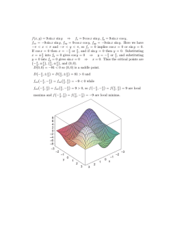
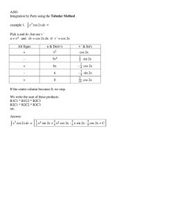
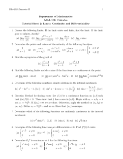
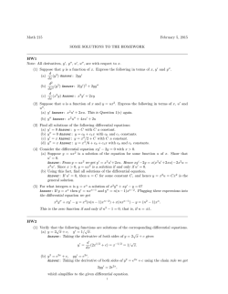
Copyright 2010 Cengage Learning. All Rights Reserved. May not be copied, scanned, or duplicated, in whole or in part. Due to electronic rights, some third party content may be suppressed from the eBook and/or eChapter(s).
Editorial review has deemed that any suppressed content does not materially affect the overall learning experience. Cengage Learning reserves the right to remove additional content at any time if subsequent rights restrictions require it.