1. Art and Diseño

Preprint Version. To appear in the Proceedings of the First Asia Pacific Bioinformatics Conference (APBC 2003)
An empirical comparison of supervised machine learning techniques in
bioinformatics
Aik Choon TAN and David GILBERT
Bioinformatics Research Centre, Department of Computing Science
12 Lilybank Gardens, University of Glasgow, Glasgow G12 8QQ, UK.
{actan, drg}@brc.dcs.gla.ac.uk
Abstract
Research in bioinformatics is driven by the experimental data.
Current biological databases are populated by vast amounts of
experimental data. Machine learning has been widely applied to
bioinformatics and has gained a lot of success in this research
area. At present, with various learning algorithms available in the
literature, researchers are facing difficulties in choosing the best
method that can apply to their data. We performed an empirical
study on 7 individual learning systems and 9 different combined
methods on 4 different biological data sets, and provide some
suggested issues to be considered when answering the following
questions: (i) How does one choose which algorithm is best
suitable for their data set? (ii) Are combined methods better than
a single approach? (iii) How does one compare the effectiveness
of a particular algorithm to the others?
Keywords: Supervised machine learning, bioinformatics,
ensemble methods, performance evaluation.
1
Introduction
In the post-genome era, research in bioinformatics has
been overwhelmed by the experimental data. The
complexity of biological data ranges from simple strings
(nucleotides and amino acids sequences) to complex
graphs (biochemical networks); from 1D (sequence data)
to 3D (protein and RNA structures). Considering the
amount and complexity of the data, it is becoming
impossible for an expert to compute and compare the
entries within the current databases. Thus, machine
learning and artificial intelligence techniques have been
widely applied in this domain to discover and mine the
knowledge in the databases. Quoting from Baldi and
Brunak (Baldi and Brunak, 2001) “As a result, the need for
computer / statistical / machine learning techniques is
today stronger rather than weaker.”
Shavlik et al. (Shavlik et al., 1995) described the field of
molecular biology as tailor-made for machine learning
approaches. This is due to the nature of machine learning
approaches that performs well in domains where there is a
vast amount of data but little theory – this is exactly the
situation in bioinformatics. Since the introduction of
machine learning to this field, various algorithms and
methods have been produced and applied to study different
data sets. Most of these studies compare a ‘new’ algorithm
Copyright © 2003, Australian Computer Society, Inc. This paper
appeared at First Asia-Pacific Bioinformatics Conference,
Adelaide, Australia. Conferences in Research and Practice in
Information Technology, Vol. 19. Yi-Ping Phoebe Chen, Ed.
Reproduction for academic, not-for profit purposes permitted
provided this text is included.
with the conventional ones, asserting the effectiveness and
efficiencies of their methods in particular data sets. The
variety of learning algorithms currently available for the
researchers are enormous and the main problems faced by
researchers are: (i) How does one choose which algorithm
is best suitable for their data set? (ii) Are combined
methods better than a single approach? (iii) How does one
compare the effectiveness of a particular algorithm to the
others?
The objective of this study is to provide some suggestions
for the community by answering the above questions. This
paper is organised as follows. Section 2 presents a brief
summary of machine learning. Section 3 outlines the
materials and methods used in this study. Section 4
presents the results and discussion, and the final section
summarises this work.
2
Machine Learning Background
A machine learning algorithm is one that can learn from
experience (observed examples) with respect to some class
of tasks and a performance measure. (Mitchell, 1997).
Machine learning methods are suitable for molecular
biology data due to the learning algorithm’s ability to
construct classifiers/hypotheses that can explain complex
relationships in the data. The classifiers or hypotheses can
then be interpreted by a domain expert who suggests some
wet-lab experiments to validate or refute the hypotheses.
This feedback loop between in silico and in vivo / in vitro
experiments accelerates the knowledge discovery process
over the biological data. This feedback is an important
characteristic of machine learning in bioinformatics.
Generally, there are two types of learning schemes in
machine learning: supervised learning where the output
has been given a priori labelled or the learner has some
prior knowledge of the data; and unsupervised learning
where no prior information is given to the learner
regarding the data or the output. The overall tasks for the
learner are to classify, characterise, and cluster the input
data. Classification is the most common task in biological
problem where given two different sets of examples,
namely positive E+ and negative E- examples (E+∩E- =∅),
the learner needs to construct a classifier to distinguish
between the positive examples and the negative set. This
classifier can then be used as the basis for classifying as
yet unseen data in the future. Usually, for a supervised
classification problem, the training examples are in the
form of a set of tuples {( x1 , y1 j ),..., ( xn , y n j )} where xi is
the class label and yij is the set of attributes for the
instances. The task of the learning algorithm is to produce
a classifier (hypothesis, function) to classify the instances
into the correct class. In this study, we only consider
supervised machine learning applied to classification.
3
3.1
Materials and Methodologies
Machine learning algorithms
We performed an empirical comparison of rule-based
learning systems (Decision trees, One Rule, Decision
rules), statistical learning system (Naïve Bayes, Instance
Based, SVM and neural networks) and ensemble methods
(Stacking, Bagging and Boosting) on the data listed in
Table 1 based on the accuracy, positive predicted value,
specificity and sensitivity of the learning algorithms. All
the learning methods used in this study were obtained from
the
WEKA
machine
learning
package
(http://www.cs.waikato.ac.nz/~ml/weka/).
3.2
Data set
In this study we used the following data sets obtained from
UCI machine learning repository (Blake and Merz, 1998).
We briefly describe the biological motivation for the data
sets; interested readers should refer to the cited papers for
details.
E.coli data set – The objective of this data set is to predict
the cellular localisation sites of E.coli proteins (Horton and
Nakai, 1996). There are 8 different cellular sites, which
are cytoplasm (cp), inner membrane without signal
sequence (im), periplasm (pp), inner membrane with
uncleavable signal sequence (imU), outer membrane (om),
outer membrane lipoprotein (omL), inner membrane
lipoprotein (imL) and inner membrane with cleavable
signal sequence (imS). The attributes are signal sequence
recognition methods (specifically those of McGeoch and
von Heijne), the presence of charge on N-terminus of
predicted lipoproteins and 3 different scoring functions on
the amino acid contents whether predicted as a outer
membrane or inner membrane, cleavable or uncleavable
sequence signal.
Yeast data set – The objective is similar to the E.coli data,
which is to determine the cellular localisation of the yeast
proteins (Horton and Nakai, 1996). There are 10 different
sites, which include: CYT (cytosolic or cytoskeletal);
NUC (nuclear); MIT (mitochondrial); ME3 (membrane
protein, no N-terminal signal); ME2 (membrane protein,
uncleaved signal); ME1 (membrane protein, cleaved
signal); EXC (extracellular); VAC (vacuolar); POX
(peroxisomal) and ERL (endoplasmic reticulum lumen).
The attributes are similar to the E.coli data set with the
addition of nuclear localisation information.
Promoter data set. The task of the classifier is to predict
whether a DNA sequence from E.coli is either a promoter
or not (Towell et al., 1990). The input data is a
57-nucleotide sequence (A, C, T or G).
HIV data set – The data set contains 362 octamer protein
sequences each of which needs to be classified as an HIV
protease cleavable site or uncleavable site (Cai and Chou,
1998).
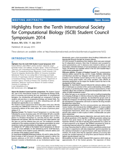
Data set
E.coli
Yeast
Promoters
HIV
Continuous Attribute
2
0
57
8
Discrete Attribute
5
8
0
0
Classes
8
10
2
2
Data Size
336
1484
106
362
Table 1: Data sets used in this study.
3.3
Evaluation
We constructed a confusion matrix (contingency table) to
evaluate the classifier’s performance. Table 2 shows a
generic contingency table for a binary class problem. True
positives (TP) denote the correct classifications of positive
examples. True negatives (TN) are the correct
classifications of negative examples. False positives (FP)
represent the incorrect classifications of negative
examples into class positive and False negatives (FN) are
the positive examples incorrectly classified into class
negative.
Predicted
Actual
Positive
Negative
Positive
TP
FN
Negative
FP
TN
Table 2: A contingency table for a binary class
problem.
Based on the contingency table, several measurements can
be carried out to evaluate the performance of the induced
classifier. The most popular performance evaluation
measure used in prediction or classification learning is
classifier accuracy which measures the proportion of
TP + TN
.
correctly classified instances; Acc =
TP + TN + FP + FN
Positive Predictive Accuracy (PPV, or the reliability of
positive predictions of the induced classifier) is computed
by PPV = TP . Sensitivity (Sn) measures the fraction of
TP+ FP
actual positive examples that are correctly classified
TP ; while specificity (Sp) measures the fraction
S =
n
TP + FN
of actual
classified S
3.4
p
negative
TN
.
=
examples
that
are
correctly
TN + FP
Cross-validation
To evaluate the robustness of the classifier, the normal
methodology is to perform cross validation on the
classifier. Ten fold cross validation has been proved to be
statistically good enough in evaluating the performance of
the classifier (Witten and Frank, 2000). In ten fold cross
validation, the training set is equally divided into 10
different subsets. Nine out of ten of the training subsets
are used to train the learner and the tenth subset is used as
the test set. The procedure is repeated ten times, with a
different subset being used as the test set.
Preprint Version. To appear in the Proceedings of the First Asia Pacific Bioinformatics Conference (APBC 2003)
4
Results and Discussion
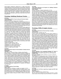
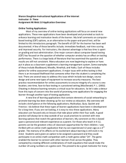
We summarise our experimental results in Figure 1 and 2.
The full analysis of this study is available in
http://www.brc.dcs.gla.ac.uk/~actan/APBC2003.
4.1
Rules-of-thumb
In this section, we address the following questions by
providing some suggested issues (rules-of-thumb) to be
considered when answering them.
(i) How does one choose which algorithm is best suitable
for their data set?
Ratio of the training data – From these experiments, we
observed that the division of the training data plays a
crucial role in determining the performance of the
algorithms. If the training TPs and TNs are almost equal in
size, the algorithms tend to construct much better
classifiers. This observation suggested that the classifier
induced from equal size of TP and TN tend to be more
robust in classifying the instances. Furthermore, the
classifiers generated consider all the discriminative
attributes that distinguish between two different classes. If
the size of the TP set is small compared to that of TN, most
probably the classifier will overfit the positive examples
and thus perform poorly in the cross validation stages.
Figure 1. Accuracy vs Positive Predictive Value
Figure 2. Specificity vs Sensitivity
From the results, we observed that most of the individual
learners tend to perform well either in accuracy or
specificity. Probably this is due to the induced classifier
being able to characterise the negative examples (most of
the training sets have large ratio of negative examples
compared to positive examples). Furthermore, the results
suggest that combination approaches are in general better
at minimising overfitting of the training data. We also
observed from this experiment that boosting performs
better than bagging. This is because attributes which are
highly important in discriminating between classes are
randomly removed by bagging; however they are
preserved in boosting and thus contribute to the final
voting scheme. The only individual learning system that
perform better than the combined methods is Naïve Bayes
learning. This may suggest that Naïve Bayes is capable of
classifying instances based on simple prior probabilistic
knowledge. In this study SVM does not perform well
compared to other methods, probably due to the fact that
training data are not separable in the vector space.
Attributes – Another factor that must be taken into
consideration when choosing a learning method is the
nature of the attributes. Generally, statistical methods (e.g.
SVM, neural networks) tend to perform much better over
multi-dimensions and continuous attributes. This is
because the learning strategy embedded in these
algorithms enables the learners to find a maximal margin
that can distinguish different classes in the vector space.
By contrast, rule-based systems (e.g. Decision trees,
PART) tend to perform better in discrete / categorical
attributes. The algorithms of these methods operate in a
top-down manner where the first step is to find the most
discriminative attribute that classifies different classes.
The process is iterated until most of the instances are
classified into their class.
Credibility vs. Comprehensibility – When choosing a
machine learning technique, users need to ask themselves
what they really want to “discover” from the data. If they
are interested in generating understandable hypotheses,
then a rule-base learning algorithm should be used instead
of statistical ones. Most machine learning algorithms
follow Occam’s principle when constructing the final
hypothesis. According to this principle, the algorithm
tends to find the simplest hypotheses by avoiding
overfitting the training data. But does this principle still
hold in bioinformatics? In bioinformatics we often wish
to explore data and explain results, and hence we are
interested in applying intelligent systems to provide an
insight to understand the relations between complex data.
The question then arises as to whether we prefer a simple
classifier or a highly comprehensible model. In general,
there is a trade off between the credibility and
comprehensibility of a model.
Domingos (1999)
suggested applying domain constraints as an alternative
for avoiding overfitting the data. We agree with
Muggleton et al. (1998) that when comparing the
performance of learning systems in a bioinformatics
context, the hypothesis with better explanatory power is
preferable when there exist more than one hypotheses with
statistical equivalent predictive accuracy.
(ii) Are combined methods better than a single approach?
From the experiments most of the combined methods
perform better than the individual learner. This is because
none of the individual methods can claim that they are
superior to the others due to statistical, computational and
representational reasons (Dietterich, 2000).
Every
learning algorithm uses a different search strategy. If the
training data is too small, the individual learner can induce
different hypotheses with similar performances from the
search space. Thus, by averaging the different hypotheses,
the combined classifier may produce a good
approximation to the true hypotheses. The computational
reason is to avoid local optima of individual search
strategy. By performing different initial searches and
combining the outputs, the final classifier may provide a
better approximation to the true hypotheses. Lastly, due to
the limited amount of training data, the individual
classifier may not represent the true hypotheses. Thus,
through considering different classifiers, it may be
possible to expand the final classifier to an approximate
representation of the true hypotheses. Ensemble learning
has been an active research topic in machine learning but
not in the bioinformatics community. Since most of the
hypotheses induced are from incomplete biological data, it
is essential to generate a good approximation by
combining individual learners.
(iii) How does one compare the effectiveness of a
particular algorithm to the others?
consistently perform well over all the data sets. The
performance of the learning techniques is highly
dependant on the nature of the training data. This study
also shows that combined methods perform better than the
individual ones in terms of their specificity, sensitivity,
positive predicted value and accuracy. We have suggested
some rules-of-thumb for the reader on choosing the best
suitable learning method for their dataset.
6
Acknowledgements
We would like to thank colleagues in the Bioinformatics
Research Centre for constructive discussions. We would
also like to thank the anonymous reviewers for their useful
comments. The University of Glasgow funded AC Tan’s
studentship.
7
References
BALDI, P. AND BRUNAK, S. (2001) Bioinformatics:
The Machine Learning Approach, 2nd Ed., MIT Press.
Blake, C.L. AND Merz, C.J. (1998) UCI Repository of
machine
learning
databases
[http://www.ics.uci.edu/~mlearn/MLRepository.html]
CAI, Y.-D. AND CHOU, K.-C. (1998) Artificial neural
network model for predicting HIV protease cleavage
sites in protein. Advances in Engineering Software, 29:
119-128.
DIETTERICH, T.G. (2000) Ensemble methods in
machine learning. In Proceedings of the First
International Workshop on MCS, LNCS 1857: 1-15.
Predictive accuracy – Most of the time, we can find in the
literature reports that a learning scheme performs better
than another in term of one model’s accuracy when
applied to a particular data set. From this study, we found
that accuracy is not the ultimate measurement when
comparing the learner’s credibility. Accuracy is just the
measurement of the total correctly classified instances.
This measurement is the overall error rate, but there can be
other measures of the accuracy of a classifier rule. If the
training data set has 95 TNs and 5 TPs, by classifying all
the instances into a negative class, the classifier still can
achieve a 95% accuracy. But the sensitivity and the
positive predicted value is 0% (both measurements
evaluate the performance in classifying TPs). This means
that although the accuracy of the classifier is 95% it still
cannot discriminate between the positive examples and the
negatives. Thus, when comparing the performance of
different classifiers, accuracy as a measure is not enough.
Different measures should be evaluated depending on
what type of question that the user seeks to answer. See
Salzberg (Salzberg, 1999) for a tutorial on comparing
classifiers.
SALZBERG, S. (1999). On comparing classifiers: a
critique of current research and methods. Data mining
and knowledge discovery, 1: 1-12.
5
SHAVLIK, J., HUNTER, L. & SEARLS, D. (1995).
Introduction. Machine Learning, 21: 5-10.
Conclusions
Machine learning has increasingly gained attention in
bioinformatics research. With the availability of different
types of learning methods, it has become common for the
researchers to apply the off-shelf systems to classify and
mine their databases. In the research reported in this paper,
we have performed a comparison of different supervised
machine learning techniques in classifying biological data.
We have shown that none of the single methods could
DOMINGOS, P. (1999) The role of Occam’s razor in
knowledge discovery. Data Mining and Knowledge
Discovery, 3: 409-425.
HORTON, P. AND NAKAI, K. (1996) A probabilistic
classification system for predicting the cellular
localization sites of proteins. In Proceedings of Fourth
International Conference on ISMB, p.109-115. AAAI /
MIT Press.
MITCHELL, T. (1997) Machine Learning. McGraw-Hill.
MUGGLETON, S., SRINIVASAN, A., KING, R.D. AND
STERNBERG, M.J.E. (1998) Biochemical knowledge
discovery using inductive logic programming. In H.
Motoda (Ed.) Proceedings of the First Conference on
Discovery Science, Springer-Verlag.
TOWELL, G.G., SHAVLIK, J.W. AND NOORDEWIER,
M.O. (1990) Refinement of approximate domain
theories by knowledge-based neural networks. In
Proceedings of the Eighth National Conference on
Artificial Intelligence, p. 861-866. AAAI Press.
WITTEN, I.H. AND FRANK, E. (2000) Data Mining:
Practical machine learning tools and techniques with
java implementations. Morgan Kaufmann.