1. Art and Diseño

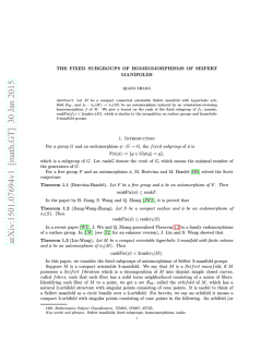
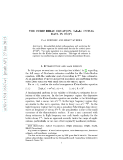
1
Structure-Based Self-Triggered Consensus in
Networks of Multiagents with Switching
arXiv:1501.07349v1 [math.OC] 29 Jan 2015
Topologies
Bo Liu Member, IEEE, Wenlian Lu Member, IEEE, Licheng Jiao Senior
Member, IEEE, and Tianping Chen Senior Member, IEEE
Abstract
In this paper, we propose a new self-triggered consensus algorithm in networks of multi-agents.
Different from existing works, which are based on the observation of states, here, each agent determines
its next update time based on its coupling structure. Both centralized and distributed approaches of the
algorithms have been discussed. By transforming the algorithm to a proper discrete-time systems without
self delays, we established a new analysis framework to prove the convergence of the algorithm. Then
we extended the algorithm to networks with switching topologies, especially stochastically switching
topologies. Compared to existing works, our algorithm is easier to understand and implement. It explicitly
provides positive lower and upper bounds for the update time interval of each agent based on its coupling
This work is jointly supported by the National Basic Research Program (973 Program) of China (No. 2013CB329402),
the National Natural Science Foundation of China(No.61473215), The Fund for Foreign Scholars in University Research
and Teaching Programs (the 111 Project) (No. B07048), National Science Foundation of China under Grant No. 91438103,
91438201, the Program for Cheung Kong Scholars and Innovative Research Team in University (No. IRT1170), the Fundamental
Research Funds for the Central Universities under Grant No. XJS14035. Marie Curie International Incoming Fellowship from the
European Commission (FP7-PEOPLE-2011-IIF-302421), the National Natural Sciences Foundation of China (Nos. 61273211
and 61273309), and the Program for New Century Excellent Talents in University (NCET-13-0139)
B. Liu and L. Jiao are with Key Laboratory of Intelligent Perception and Image Understanding of Ministry of Education,
International Research Center for Intelligent Perception and Computation, Xidian University, Xi’an, Shaanxi Province 710071,
China (email: [email protected], [email protected]); W. Lu is with the Centre for Computational Systems Biology
and School of Mathematical Sciences, Fudan University, Shanghai, 200433, China(email: [email protected]); T. Chen is
with the School of Computer Science and School of Mathematical Sciences, Fudan University, Shanghai 200433, China(Email:
[email protected]).
January 30, 2015
DRAFT
structure, which can also be independently adjusted by each agent according to its own situation. Our
work reveals that the event/self triggered algorithms are essentially discrete and more suitable to a
discrete analysis framework. Numerical simulations are also provided to illustrate the theoretical results.
Key words: self-triggered, distributed, consensus, switching topology.
I. I NTRODUCTION
Distributed control of networked cooperative multiagent systems has received much attention in
recent years due to the rapid advances in computing and communication technologies. Examples
include agreement or consensus problems [1]–[3], in which a group of agents seek to agree upon
certain quantities of interest, formation control of robots and vehicles [4], [5], and distributed
estimation [6], [7], etc.
In these applications, an important aspect is to determine the controller actuation schemes.
Although continuous feedback of states have always been used in early implementations of
distributed control, it is not suitable for agents equipped with embedded microprocessors that
have very limited resources to transmit and gather information. To overcome this difficulty,
event-triggered control scheme [8]–[16] was proposed to reduce the controller updates. In fact,
event-driven strategies for multi-agent systems can be viewed as a linearization and discretization
process, which was considered and investigated in early papers [17], [18]. For example, in the
paper [17], following algorithm was investigated
xi (t + 1) = f (xi (t)) + ci
m
X
aij (f (xj (t)))
(1)
j=1
which can be considered as nonlinear consensus algorithm. In particular, let f (x(t)) = x(t) and
ci = (tik+1 − tik ). Then (1) becomes
i
x
(tik+1 )
i
=x
(tik )
+
(tik+1
−
tik )
m
X
aij xj (tik ),
(2)
j=1
which is some variant of the event triggering (distributed, self triggered) model for consensus
problem. In centralized control, the bound for (tik+1 − tik ) = (tk+1 − tk ) to reach synchronization
was given in the paper [17] when the coupling graph is indirected and in [18] for the directed
coupling graph. The key point in event-triggered algorithm is the design of a decision maker that
2
determines when the next actuator update should occur. The existing event-triggered algorithms
are all based on the observation of states. For example, in a typical event-triggered algorithm
proposed in [8], an update is triggered when a certain error of the states becomes large enough
with respect to the norm of the state, which requires a continuous observation of the states.
In addition, self-triggered control [19]–[23] has been proposed as a natural extension of eventtriggered control, in which each agent predicts its next update time based on discontinuous state
observation to further reduce resource usage for the control systems.
Both the event-triggered and self-triggered control algorithms that have been proposed till
now have some drawbacks in common. First, the resulting system in event-triggered control is
one that with system delays, especially with self delays, which generally is difficult to handle.
And the existing analysis for such algorithms are always based on some quadratic Lyapunov
function, which has very strict restrictions on the network structure. For example, to the best
of our knowledge, the latest analysis is still restricted to static networks. Second, since these
algorithms are based on the observation of states, which are generally much complicated and
untraceable, making it difficult to predict and exclude some unexpected possibilities such as the
occurrence of zero inter-execution times.
To overcome such difficulties, we proposed a new kind of self-triggered consensus algorithms
that are structure-based. That is, each agent predicts its next update time based on its coupling
structure with its neighbours instead of the observation of their states. This can bring several
advantages. First, since the coupling structure is relatively simpler and more traceable than the
states, it is relatively easier to handle. Actually, in our algorithm, the occurrence of zero interexecution time has been excluded by directly providing a positive lower bound on the update
intervals.
Second, although the resulting system of the self-triggered algorithm is one with self delays,
by some proper transformation, we showed that the system can corresponding to a discrete-time
system without self-delays. We have proposed the algorithm in both centralized and distributed
approaches. In the centralized approach, the system can be directly related to a discrete-time
system without delays, which can be seen as a discrete version of the nominal system. However,
in the distributed approach, the situation is much more complicated and the system can not
be directly transformed into its discretized version. However, by some proper indirect transformation, we showed that the convergence of the nominal system can be reduced to that of a
3
discrete-time consensus algorithm with off-diagonal delays but without self delays. Thus, other
than using a quadratic Lyapunov function, the convergence of the original algorithm can be
solved by the analysis of a discrete-time consensus algorithm. This brings another possibility
that is also considered as a big advantage and a major contribution of this work. That is, we can
analyze networks with switching topologies, especially stochastically switching topologies.
The rest of the paper is organized as follows: Section II provides some preliminaries on
matrix and graph theory that will be used in the main text. Section III provides the self-triggered
consensus algorithm in both centralized and distributed approach with convergence analysis.
Section IV provide an example with numerical simulation to illustrate the theoretical results
obtained in the previous section. The paper is concluded in Section V.
II. P RELIMINARIES
In this section, we present some definitions and results in matrix and graph theories and
probability theories that will be used later.
For a matrix A = [aij ], aij represents the entry of A on the ith row and jth column, which is
sometimes also denoted as [A]ij . A matrix A = [aij ] is called a nonnegative matrix if aij ≥ 0
P
for all i, j. And A is called a stochastic matrix if A is square and j aij = 1 for each i. Given
a nonnegative matrix A and δ > 0, the δ-matrix of A is a matrix that has nonzero entries only
in the place that A has entries equal to or greater than δ. For two matrix A, B of the same
dimension, we write A ≥ B if A − B is a nonnegative matrix. Throughout this paper, we use
Qk
i=1 Ai = Ak Ak−1 · · · A1 to denote the left product of matrices.
A directed graph G is defined by its vertex set V(G) = {v1 , · · · , vn } and edge set E(G) ⊆
{(vi , vj ) : vi , vj ∈ V(G)}, where an edge is an ordered pair of vertices in V(G). If (vi , vj ) ∈
E(G), then vi is called the (in-)neighbour of vj . Ni = {j : (vj , vi ) ∈ E(G)} is the set of
neighbours of agent i. A directed path in G is an ordered sequence of vertices v1 , · · · , vs such
that (vi , vi+1 ) ∈ E(G) for i = 1, · · · , s − 1. A directed tree is a directed graph where every
vertex has exactly one in-neighbour except one ,called the root, without any in-neighbour. And
there exists a directed path from the root to any other vertex of the graph. A subgraph of G is
a directed graph GS satisfying V(GS ) ⊆ V(G), and E(G) ⊆ E(G). A spanning subgraph of G is
a subgraph of G that has the same vertex set with G. We say G has a spanning tree if G has a
spanning subgraph that is a tree.
4
A weighted directed graph is a directed graph where each edge is equipped with a weight.
Thus, a graph G of n vertices corresponds to an n × n nonnegative matrix A = [aij ], called
the weight matrix in such way that (vj , vi ) ∈ E(G) if and only if aij > 0. On the other hand,
given an n × n nonnegative matrix A, it corresponds to a weighted directed graph G(A) such
that G(A) has A as its weight matrix. Using this correspondence, we can introduce the concept
of δ-graph. The δ-graph of G is a weighted directed graph that has the δ-matrix of G’s weight
matrix as its weight matrix. A graph G has a δ spanning tree if its δ-graph has a spanning tree.
From the weight matrix A = [aij ] of a graph G, we define its graph Laplacian L = [lij ] as
follows:
lij =

 P
k6=i

aik , i = j;
−aij ,
i 6= j.
Thus L has zero row sum with lii > 0 while lij ≤ 0 for i, j = 1, 2, · · · , n and i 6= j. And
the nonnegative linear combination of several graph Laplacians is also a graph Laplacian of
some graph. There is a one-to-one correspondence between a graph and its weight matrix or its
Laplacian matrix. In the following, for the sake of simplicity in presentation, sometimes we don’t
explicitly distinguish a graph from its weight matrix or Laplacian matrix, i.e., when we say a
matrix has some property that is usually associated with a graph, what we mean is that property
is held by the graph corresponding to this matrix. For example, when we say a nonnegative
matrix A has a spanning tree, what we mean is that the graph of A has a spanning tree. And
it is of similar meaning when we say that a graph has some property that is usually associated
with a matrix.
Let {Ω, F , P} be a probability space, where Ω is the sample space, F is σ-algebra on Ω, and
P is the probability on F . We use E{·} to denote the mathematical expectation and E{·|F } the
conditional expectation with respect to F , i.e., E{·|F } is a random variable that is measurable
with respect to F .
Definition 1 (adapted process/sequence): Let {Ak } be a stochastic process defined on the
basic probability space {Ω, F , P}, and let {Fk } be a filtration, i.e., a sequence of nondecreasing
sub-σ-algebras of F . If Ak is measurable with respect to Fk , then the sequence {Ak , Fk } is
called an adapted process/sequence.
Remark 1: For example, let X(ω) be a random variable defined on Ω, then {E{X(ω)|Fk }, Fk }
is an adapted sequence.
5
III. S ELF -T RIGGERED C ONSENSUS A LGORITHM
In a network of n agents, with xi ∈ R being the state of agent i, we assume that each agent’s
dynamics obey a single integrator model
x˙ i (t) = ui (t), i = 1, 2, · · · , n,
(3)
where ui (t) is the control law for agent i at time t. In consensus algorithm, the control law is
usually given by( [1], [29], [30])
ui (t) = −
X
lij [xj (t) − xi (t)] = −
n
X
lij [xj (t) − xi (t)].
(4)
j=1
j∈Ni
Thus the consensus algorithm can be written as
x˙ i (t) = −
n
X
lij [xj (t) − xi (t)],
(5)
j=1
or in matrix form as
x(t)
˙
= −Lx(t),
(6)
where x(t) = [x1 (t), · · · , xn (t)]⊤ ∈ Rn is the stack vector of the agents’ states. In event/selftriggered control, the control law u(t) is piecewise constant, i.e.,
u(t) = u(tk ), t ∈ [tk , tk+1 ),
(7)
where {tk } is the time sequence that an update of u(·) occurs. The central point of such algorithm
is the choice of appropriate {tk } such that some desired properties of the algorithm such as
stability and convergence can be preserved. This can be done in a centralized approach or a
distributed approach, both of which will be discussed in the following.
A. Centralized Approach
In this subsection, we first consider centralized self-triggered consensus algorithm. The sequence of the update time is denoted by: t0 , t1 , t2 , · · · , then the self-triggered algorithm has the
form:
x(t)
˙
= −Lx(tk ), t ∈ [tk , tk+1 ).
Denote ∆tk = tk+1 − tk for k = 0, 1, · · · . We have the following Theorem.
6
(8)
Theorem 1: If the graph G(L) has a spanning tree and there exists δ ∈ (0, 1/2) such that
δ/lmax ≤ ∆tk ≤ (1 − δ)/lmax for each k, where lmax = maxi {lii }, then the algorithm will
achieve consensus asymptotically.
Proof: From the algorithm, for each t ∈ (tk , tk+1], since
x(t)
˙
= −Lx(tk ),
we have
x(t) = x(tk ) − (t − tk )Lx(tk ) = [I − (t − tk )L]x(tk ).
Particularly, let t = tk+1 , we have
x(tk+1 ) = (I − ∆tk L)x(tk ) = Ak x(tk ),
where Ak = I − ∆tk L. It is easy to verify that Ak is a stochastic matrix for each k. In fact,
since δ/lmax ≤ ∆tk ≤ (1 − δ)/lmax ,
[Ak ]ii = 1 − ∆tk lii ≥ 1 − ∆tk lmax ≥ 1 −
1−δ
lmax = δ.
lmax
For i 6= j,
[Ak ]ij = −∆tk lij ≥ 0.
It implies that [Ak ]ij is positive if and only if −lij is positive, and the positive elements of [Ak ]
is uniformly lower bounded by a positive scalar since both ∆tk and −lij is uniformly lower
P
P
bounded by a positive scalar. Furthermore, nj=1[Ak ]ij = 1 − ∆tk nj=1 lij = 1. By a standard
argument from the theory of products of stochastic matrices, there exists x∗ ∈ R such that
lim xi (tk ) = x∗ .
k→+∞
On the other hand, it is not difficult to verify that the function maxi {xi (t)} is nonincreasing and
mini {xi (t)} is nondecreasing. Thus,
lim xi (t) = x∗ .
t→+∞
Using a similar argument as that in Theorem 1, it is not difficult to propose a centralized eventtriggered algorithm on networks with stochastic switching topologies. For example, consider the
following consensus algorithm:
x(t)
˙
= −Lk x(tk ), t ∈ [tk , tk+1),
7
(9)
k
k
where Lk = [lij
] is uniformly bounded in k and lmax
= maxi {liik } ∈ [lmin , lmax ] for some
0 < lmin < lmax . Before provide the next theorem, we first summarize the following assumption.
Assumption 1:
k
k
(i) There exists δ ∈ (0, 1/2) such that ∆tk ∈ [δ/lmax
, (1 − δ)/lmax
];
(ii) {Lk , Fk } is an adapted random sequence, and there exists h > 0, δ ′ > 0 such that the
Pk+h
Lm |Fk } has a δ ′ -spanning
graph corresponding to the conditional expectation E{ m=k+1
tree;
Now we have
Theorem 2: Under assumption1, the self-triggered consensus algorithm (9) will reach consensus almost surely.
Proof: Similar as in the proof of Theorem 1, we have x(tk+1 ) = Ak x(tk ) with Ak =
I − ∆tk Lk . Since {∆tk } is a deterministic sequence, {Ak , Fk } is also an adapted sequence, and
E{
k+h
X
k+h
X
Am |Fk } = hI − E{
m=k+1
∆tm Lm |Fk }
m=k+1
≥ hδI −
δ
lmax
E{
k+h
X
Lm
0 |Fk },
m=k+1
m
m
where [Lm
0 ]ij = [L ]ij for i 6= j and [L0 ]ii = 0 for all i. Thus, E{
Pk+h
m=k+1
Am |Fk } has a
δ ′′ -spanning tree with δ ′′ = δ ′ δ/lmax > 0. From Theorem 3.1 of [28], the sequence {x(tk )} will
reach consensus almost surely, thus x(t) will also reach consensus almost surely.
As corollaries in special cases, it can be shown that almost sure consensus still holds if we
replace item (ii) in Assumption 1 with one of the following more special ones.
(ii’) {Lk } is an independent and identically distributed sequence, and there exists δ ′ > 0 such
that the graph corresponding to the expectation E Lk has a δ ′ -spanning tree;
(ii”) {Lk } is a homogenous Markov chain with a stationary distribution π, and there exists
δ ′ > 0 such that the graph corresponding to the expectation with respect to π, Eπ Lk , has
a δ ′ -spanning tree;
B. Distributed Approach
In this section, we discuss the distributed event-triggered consensus algorithm.
k
Let {tki }+∞
k=0 be the time sequence such that ti is the kth time that agent i updates its control
8
law. Then the distributed self-triggered algorithm has the following form:
xi (t) = −
n
X
k (t)
lij xj (tj j ), i = 1, · · · , n,
(10)
j=1
where kj (t) = max{k : tkj ≤ t}.
− tki . Then we have the following Theorem.
Denote ∆tki = tk+1
i
Theorem 3: If the graph G(L) has a spanning tree and there exists δi ∈ (0, 1/2) for i =
1, 2, · · · , n such that ∆tki ∈ [δi /lii , (1 − δi )/lii ], then the distributed event triggered algorithm
can reach a consensus as t → ∞.
The proof will be divided into two steps corresponding to two lemmas. Now we give and
prove the first lemma.
Lemma 1: If there exists x∗ ∈ R such that
lim x(tki ) = x∗ , i = 1, 2, · · · , n,
k→∞
then the distributed event-triggered algorithm will reach a consensus, i.e.,
lim xi (t) = x∗ , i = 1, 2, · · · , n.
t→∞
Proof: By the definition of the algorithm, for agent i,
x˙ i (t) = −
n
X
k (t)
lij x(tj j )
n
X
=−
k (t)
k (t)
lij [xj (tj j ) − xi (ti i )].
j=1,j6=i
j=1
Since limt→∞ kj (t) = +∞,
lim x˙ i (t) = −
t→∞
n
X
lij (x∗ − x∗ ) = 0.
j=1,j6=i
Thus,
k (t)
k (t)
lim |xi (t) − x∗ | ≤ lim |xi (t) − xi (ti i )| + lim |xi (ti i ) − x∗ |
t→∞
t→∞
t→∞
k (t)
≤ lim ∆ti i
t→∞
≤
k (t)
max |x˙ i (s)| + lim |xi (ti i ) − x∗ |
k (t)
s∈[ti i ,t]
t→∞
1 − δi
k (t)
lim max |x˙ i (s)| + lim |xi (ti i ) − x∗ |
t→∞
lii t→∞ s∈[tki i (t) ,t]
= 0.
Now we are to provide and prove the second lemma.
9
Lemma 2: Under the assumption in Theorem 3, there exists x∗ such that
lim xi (tki ) = x∗ .
k→∞
Proof: Let {tk } be the time sequence that the kth update occurred in the network, i.e.,
{tk } = ∪ni=1 {tki }, and ∆tk = tk+1 − tk . In case for that tk = tki = tkj for some some k, k ′ ,
′
′
′′
k ′′ and i 6= j, we consider the update of agent i and j at time tk as one update of the network.
Now, construct an auxiliary sequence {y(k)}, where y(k) = [y1 (k), y2 (k), · · · , yn (k)]⊤ ∈ Rn
k (tk )
with yi (k) = xi (ti i
), i.e., yi (k) is the latest state that agent i uses in its control law at time
tk . Now consider the evolution of {y(k)}.
Case 1. Agent i does not update at time tk+1 : In this case, by definition,
yi (k + 1) = yi (k);
k (tk+1 )
Case 2. Agent i does update at time tk+1 : In this case, ti i
k (tk )
= tk+1 , assume ti i
= tk−dik be
the last update of agent i before tk+1 , with dik ≥ 0 being the number of updates occur at all
other agents xj , j 6= i, between the two successive updates of agent i, i.e., in the interval
P
)
k (t ) k (t
(ti i k , ti i k+1 ). By definition yi (k) = · · · = yi (k − dik ), and x˙ i (t) = − nj=1 lij yj (k ′ ) for
k (tk )
t ∈ (tk′ , tk′+1 ) for all k ′ . Since [ti i
k (tk+1 )
, ti i
10
) = ∪km=k−dik [tm , tm+1 ),
yi (k + 1) = xi (tk+1 ) =
k (t )
xi (ti i k )
= xi (tk−dik ) +
dik Z
X
= xi (tk−dik ) −
k (tk+1 )
ti i
k−dik +m+1
x˙ i (t)dt
∆tk−dik +m
m=0
= yi (k − dik ) −
x˙ i (t)dt
k (tk )
ti i
tk−dik +m
m=0
dik
X
+
Z
n
X
lij yj (k − dik + m)
j=1
dik
X
∆tk−dik +m lii yi (k − dik + m)
m=0
−
dik
X
∆tk−dik +m
m=0
n
X
lij yj (k − dik + m)
j=1,j6=i
dik
X
= yi (k) −
∆tk−dik +m lii yi (k) −
m=0
= (1 − lii
dik
X
∆tk−dik +m
m=0
∆tk−dik +m )yi (k) −
dik
X
n
X
lij yj (k − dik + m)
j=1,j6=i
n
X
∆tk−dik +m lij yj (k − dik + m)
m=0 j=1,j6=i
m=0
= (1 −
dik
X
k (t )
∆ti i k lii )yi (k)
−
dik
n
X
X
∆tk−dik +m lij yj (k − dik + m)
m=0 j=1,j6=i
=
dik X
n
X
am
ij (k)yj (k − m),
m=0 j=1
k (tk )
where a0ii (k) = 1 − ∆ti i
m
lii , am
ii (k) = 0 for m = 1, 2, · · · , dik and aij (k) = −∆tk−m lij .
k (tk )
It is easy to verify that a0ii (k) = 1 − ∆ti i
and
dik X
n
X
lii ≥ 1 − (1 − δi ) = δi , am
ij = −∆tk−m lij ≥ 0,
am
ij (k) = 1.
m=0 j=1
Besides, by the assumption δi /lii ≤ ∆tki ≤ (1 − δi )/lii for each i, k, it is clear that
in the interval [tki , tk+1
], only finite updates occur for agents xj with j 6= i, and the
i
number of updates is uniformly upper bounded, i.e., there exists τ > 0 independent of
i, k, such that dik ≤ τ . For example, let δmin = mini {δi /lii }, and δmax = maxi {δi /lii },
then δmin ≤ ∆tki ≤ δmax for all i, k, and on each time interval of length mδmin , at most
m + 1 updates occur for each agent. Let h′ be the smallest positive integer satisfying
11
h′ δmin ≥ δmax , then on each time interval of length δmax , at most h′ + 1 updates occur for
each agent. Thus on the interval (tki , tk+1
), at most (n − 1)(h′ + 1) updates occur for all
i
agents j with i 6= j. Pick τ = (n − 1)(h′ + 1), then dik ≤ τ for all i, k.
If agent i does not update at time tk+1 , i.e., case 1, we define am
ij (k) = 0 for all m = 0, 1, · · · , τ
and i, j = 1, 2, · · · , n except for a0ii (k) = 1,
If agent i updates at time tk+1 , i.e., case 2, we define am
ij (k) = 0 for all i, j = 1, 2, · · · , n and
m = dik + 1, · · · , τ when dik < τ .
For both cases, we can give a uniform iterative formula for y(k) as:
y(k + 1) =
τ X
n
X
alij (k)yj (k − l),
(11)
l=0 j=1
where alij (k) ≥ 0 for all i, j, l, k, and
τ X
n
X
alij (k) = 1,
l=0 j=1
for all i, k. Denote δ = mini {δi } > 0, we have a0ii (k) ≥ δ for all i, k.
Construct a new matrix B(k) = [bij (k)], where
bii (k) = a0ii (k)
(12)
and
bij (k) =
τ
X
alij (k), if i 6= j
(13)
l=0
k (tk )
Obviously, B(k) ≥ δI, and bij (k) = ∆ti i
lij ≥ δmin lij if agent i updates at time tk+1 .
If there exists h > 0 such that on each interval [tk , tk+h ] all agents update at least once, then
Pk+h
′
m=k B(m) ≥ −δmin L for each k. Since G(L) has a spanning tree, there exists δ > 0 such that
Pk+h
′
m=k B(m) has a δ -spanning tree for each k. From Corollary 2 in the appendix, the sequence
{y(k)} will reach a consensus, i.e., there exists x∗ ∈ R such that
lim yi (k) = x∗ .
k→∞
This is equivalent to
lim xi (tki ) = x∗ .
k→∞
At last, we give some hint on how to calculate the quantity h mentioned above. It is easy to see
that each agent updates at least once on each time interval of length δmax , since ∆tki ≤ δmax for
12
all i, k. And in each time interval of length δmax , there are at most n(h′ + 1) updates of all the
agents, where h′ is defined as before. Pick h = n(h′ + 1), then for each k, each agent updates
at least once in the time interval [tk , tk+h ].
Remark 2: It is not difficult to see that this algorithm is applicable to leader-follower networks,
in which the leader receives no information from others. For example, if agent i is the leader,
then lii = 0 and the update time interval ∆t0i = +∞ by definition, which mean the leader i does
not need to update its state. Generally, if agent i wants a long update time interval, all it needs
to do is to choose small coupling weights so that lii is small, and this can be done independent
of all other agents.
From the above analysis, it is not difficult to see that the distributed event-triggered algorithm
can also be applied to networks with switching topologies. For example, at each update time tki ,
agent i may reset its coupling weights lij such that the algorithm can be written in the form:
n
X
k (t)
k
x˙ i (t) = −
lij
xj (tj j ), t ∈ [tki , tk+1
), i = 1, 2, · · · , n,
(14)
i
j=1
where
δi /liik
≤
∆tki
≤ (1 − δi )/liik . One of the great advantage of this algorithm is that each
agent can adjust its update time interval independently based on its own need. If agent i wants
a longer update time interval, then it may decrease the coupling weight, otherwise, increase the
coupling weight. For example, each agent i may store a scaling factor ǫki such that
k
lij
= ǫki lij .
(15)
By a similar analysis as in the case of fixed topology, we can prove
Theorem 4: Suppose that ǫmin and ǫmax are two positive number satisfying 0 < ǫmin < ǫmax
and for all i, k, ǫmin ≤ ǫki ≤ ǫmax . If the graph G(L) has a spanning tree, then the distributed
event-triggered consensus algorithm with switching topology (14) and weight updating rule (15)
can reach consensus as t → ∞.
Finally, we investigate event-triggered consensus algorithm in networks with stochastically
switching topologies in which each agent i updates its coupling weights independently at the
same time it updates its state.
Given 0 < a < b, and let Si (a, b) = {s = [s1 , · · · , sn ] : si ∈ [a, b], sj ≤ 0, j 6= i,
0}. The event-triggered algorithm can be formulated as follows:
n
X
˜lk xj (tkj (t) ), t ∈ [tk , tk+1 ),
x˙ i (t) = −
ij
i i
j
j=1
13
Pn
j=1 sj
=
(16)
˜ k = [˜lk , · · · , ˜lk ] ∈ Si (ai , bi ) for some given 0 < ai < bi , and {L
˜ k } is an independent
where L
i
i1
in
i
and identically distributed sequence. Before stating the convergence result, we summarize the
following assumption.
(i) There exist δi ∈ (0, 1/2) such that ∆tki ∈ [δi /˜liik , (1 − δi )/˜liik ];
˜ k has a δ-spanning tree,
(ii) There exists δ > 0 such that the graph with Laplacian being E L
˜ k = [L
˜ k⊤
˜ k⊤ ⊤
˜k
where L
1 , · · · , Ln ] is a matrix with its ith row being Li ;
Assumption 2:
Theorem 5: Under Assumption 2, the event-triggered consensus algorithm (16) will reach a
consensus almost surely.
Proof: The algorithm (16) can be reformulated as:
x˙ i (t) = −
n
X
k (t)
k
lij
xj (tj j ), t ∈ [tk , tk+1 ),
(17)
j=1
k
where lij
=
˜lki (tk ) .
ij
k
Let Lk = [lij
], then generally the sequence {Lk } is not an independent
k+1
k
sequence since for each k, lij
= lij
if no update of agent i occurs at time tk+1 . However,
similar to the analysis given above, it can be seen that Lk is independent of Lk for k ′ ≥ k + N,
′
where N = n(h′ +1) and h′ is the smallest positive integer satisfying h′ mini {δi /bi } ≥ maxi {(1−
δi )/ai }.
Similarly, we have
y(k + 1) =
N X
n
X
alij (k)yj (k − l),
(18)
l=0 j=1
where
alij (k)
≥ 0 for all i, j, l, k, and
N X
n
X
alij (k) = 1,
l=0 j=1
for all i, k. Since
alij (k)
=
k−l
−∆tk−l lij
,
we can see that A0 (k), · · · , AN (k) are independent of
A0 (k ′ ), · · · , AN (k ′ ), when k ′ ≥ k + 2N. On the other hand, in each time interval (tk , tk+N ),
each agent there at least updates once. Thus we have
k+N
X
˜0,
E B(k) ≥ δ ′ L
m=k+1
˜ 0 ]ij =
where B(k) is defined as before and δ ′ = mini,k {∆tki } = mini {δi /bi } > 0, and [L
P
˜ k ]ij for i 6= j and [L
˜ 0 ]ii = 0 for all i. This implies that k+N E B(k) has a δ ′′ -spanning
−[E L
m=k+1
tree with δ ′′ = δδ ′ > 0. The conclusion follows from Corollary 3 in the Appendix.
14
IV. N UMERICAL S IMULATION
In this section, we provide an example to illustrate the theoretical results in the previous section. We use the distributed event-triggered algorithm in networks with stochastically switching
topologies as considered in Theorem 5.
Consider a network of four agents with
˜ k1 ∈ {[1, −1, 0, 0], [1, 0, 0, −1]},
L
˜ k = {[−1, 1, 0, 0], [0, 1, −1, 0]},
L
2
˜ k ∈ {[0, −1, 1, 0], [0, 0, 1, −1]},
L
3
˜ k4 ∈ {[0, −1, 0, 1], [0, 0, −1, 1]},
L
and each agent selects its coupling weights using a uniform distribution. We choose δi = 0.1
for all the agents. The next update time is randomly chosen from the permissible range. It is
not difficult to verify that the conditions in Theorem 5 are satisfied. The simulation results are
provided in Fig. 1 with the initial value of the four agents being randomly chosen. It can be
seen that the agents actually reached consensus.
V. C ONCLUSION
In this paper, we proposed a new structure-based self-triggered consensus algorithm in both
centralized approach and distributed approach. Different from existing works that used a quadratic
Lyapunov function as the analysis tool, we reduce the self-triggered consensus algorithm to a
discrete-time consensus algorithm by some proper transformation, which enables the application
of the product theory of stochastic matrices to the convergence analysis. Compared to existing
work, our method provides several advantages. First, each agent does not need to calculate
the system error to determine its update time. Second, it provides explicit positive lower and
upper bounds for the update interval of each agent based on its coupling weights, which can
be adjusted by each agent independent of other agents. We also used our method to investigate
networks with switching topologies, especially networks with stochastically switching topologies.
Our work reveals that the event/self-triggered algorithms are essentially discrete and thus more
15
20
15
xi(t)
10
5
0
−5
0
5
10
15
20
25
time (t)
Fig. 1.
Self-triggered consensus in networks of four agents with stochastically switching topologies.
suitable to a discrete analysis framework. And it is predictable that more results can be obtained
for self-triggered algorithms under our new analysis framework in the future.
A PPENDIX : D ISCRETE - TIME
CONSENSUS ANALYSIS
The appendix is devoted to the discussion of discrete-time consensus algorithms in networks
of multi-agents with time delays based on the product theory of stochastic matrices and provide
some results that is used in the main text.
A. Preliminaries
This subsection will provide some preliminaries on stochastic matrices that will be used in
the proof of Theorem 6 in the next subsection.
A nonnegative matrix A is called a stochastic indecomposable and aperiodic (SIA) if it is a
stochastic matrix and there exists a column vector v such that limk→∞ Ak = en v ⊤ , where en is
an n-dimensional column vector with all entries 1. A sequence of stochastic matrices {Ak } is
16
ergodic if there exists a column vector v such that limk→∞
Q∞
k=1
Ak = en v ⊤ . A is called δ-SIA
if its δ-matrix is SIA. A stochastic matrix A is called scrambling if for any pair (i, j), there
exists an index k such that both aik > 0 and ajk > 0. Similarly, A is called δ-scrambling if its
δ-matrix is scrambling. For a matrix A, diag(A) refers to the diagonal matrix formed by the
diagonal elements of A, i.e., [diag(A)]ii = [A]ii for all i and [diag(A)]ij = 0 for i 6= j. And we
define diag(A) = A − diag(A).
We use P{·|F } to denote the conditional probability with respect to F on a probability space
{Ω, P, F }, which can also be expressed into the conditional expectation of an indicator function,
i.e., P{·|F } = E{1{·} |F }, where 1{·} is an indicator function which is defined as

 1, x ∈ S,
1S (x) =
 0, x 6∈ S.
Thus, P{·|F } is also a random variable that is measurable with respect to F .
In the following, we will introduce some lemmas that will be used in the proof of the main
results.
Let A = [aij ] be an n × n stochastic matrix. Define
∆(A) = max max |ai1 j − ai2 j |.
j
i1 ,i2
It can be seen that ∆(A) measures how different the rows of A are. ∆(A) = 0 if and only if
the rows of A are identical. Define
λ(A) = 1 − min
i1 ,i2
X
min{ai1 j , ai2 j }.
j
Remark 3: It can be seen that if A is scrambling, then λ < 1, if A is δ-scrambling for some
δ > 0, then λ(A) ≤ 1 − δ.
Lemma 3: [24] For any stochastic matrices A1 , A2 , · · · , Ak , k > 0,
∆(A1 A2 · · · Ak ) ≤
k
Y
λ(Ai ).
i=1
Remark 4: From Lemma 3, it can be seen that for a sequence of stochastic matrices {Ak }, if
Qki+1
Q
there exists a sequence {ki } such that ki < ki+1 , limi→∞ ki = ∞, and ∞
i=1 λ( m=ki +1 Am ) = 0,
Q
then limk→∞ ∆( km=1 Am ) = 0, i.e., {Ak } is ergodic. Particularly, from the property of scrablingQki+1
ness, if there exists δ > 0 such that there are infinite matrices in the sequence { m=k
Am }
i +1
that are δ-scrambling, then {Ak } is ergodic.
17
Lemma 4: [24], [26] Let A1 , A2 , · · · , Ak (repetitions permitted) be r × r SIA matrices with
Q2
Q
the property that for any 1 < k1 < k2 ≤ k, ki=k
Ai is SIA. If k > n(r), then ki=1 Ai is a
1
scrambling matrix. Here n(r) is the number of different types of all r × r stochastic matrices.
Lemma 5: [26] Let A1 , · · · , Am be

A1

 0

D=
 ···

0
n × n nonnegative matrices, let

A2 · · · Am

0 ··· 0 

,

..
. ··· 
···

0 ··· 0
mn×mn
let





M0 = 




I 0 ··· 0 0


I 0 ··· 0 0 


0 I ··· 0 0 


.. .. . .
. 0 0 
. .

0 0 ··· I 0
,
mn×mn
and let Mk = D + M0k for any k ∈ {1, 2, · · · , m − 1}. Then if G(
Pm
i=1
Ai ) contains a spanning
tree, then G(Mk ) contains a spanning tree with the property that the root vertex of the spanning
tree has a self-loop in G(Mk ).

I 0 ··· 0



=





I
0
·
·
·
0

Remark 5: Actually, since M0k = M0m−1
for all k ≥ m − 1, thus Lemma
.. .. . . .. 
. . 
. .

I 0 ··· 0
5 holds for all k ∈ N. This is important for our further results based on this lemma.
P
Remark 6: If the condition is G( m
i=1 Ai ) has a δ-spanning tree for some δ > 0, then the
conclusion becomes that G(Mk ) has a δ ′ -spanning tree whose root vertex has a self-loop, where
δ ′ ≥ δ/m.
Lemma 6: [25] Let A be a stochastic matrix. If G(A) contains a spanning tree with the
property that the root vertex of the spanning tree has a self-loop in G(A), then A is SIA.
From Lemma 5 and 6, we can have the following Lemma.
18
Lemma 7: Let Ai1 , · · · , Aim , i = 1, · · · , k

Ai1 Ai2

 0
0

Di = 
 ··· ···

0
0
be n × n nonnegative matrices. Let

· · · Aim

··· 0 

,

..
. ··· 

··· 0
mn×mn
Pk Pm
and M0 being defined as in Lemma 5. Then if G( i=1 j=1 Aij ) has a δ-spanning tree for some
Q
δ > 0, then the product ki=1 (Di + M0 ) has a δ ′ -spanning tree for some 0 < δ ′ < δ. And the
Q
root of the spanning tree has a self-loop, thus ki=1 (Di + M0 ) is δ ′ -SIA.
Remark 7: It is obvious from Lemma 5 that if there exists ǫ > 0 such that Di′ ≥ ǫ(M0 + Di ),
Q
then ki=1 Di′ is δ ′ -SIA for some 0 < δ ′ < δ. This is the case that will appear in the proof of
Theorem 6.
Proof: First, we have
k
k
k
Y
X
X
k
k−i
i−1
k
(M0 + Di ) ≥ M0 +
M0 Di M0 ≥ M0 +
Di M0i−1 ,
i=1
i=1
(19)
i=1
where the second inequality is due to the fact that
M0j Di
≥ Di for any j ≥ 0. And it is not
difficult to verify that the first block row sum of Di is preserved in Di M0i−1 for i = 1, · · · , k.
P
P
P P
i
Thus the first block row sum of ki=1 Di M0i−1 equals that of ki=1 Di , i.e., ki=1 m
j=1 Aj . This
P
P
means G( ki=1 Di M0i−1 ) has a δ-spanning tree. From Lemma 5, G(M0k + ki=1 Di M0i−1 ) has a
δ ′ -spanning tree for some 0 < δ ′ < δ, and the root has a self-loop. This is also true for the
Q
Q
product ki=1 (M0 + Di ) due to (19). Thus, ki=1 (M0 + Di ) is δ ′ -SIA from Lemma 6. The proof
is completed.
From Lemma 7, we can easily obtain the following corollary.
Corollary 1: Let Ai1 , · · · , Aim , i = 1, 2, · · · , be uniformly bounded n×n nonnegative matrices.
P P
i
Let Di and M0 be defined as in Lemma 7. If there exists k such that G( ki=1 m
j=1 Aj ) has a
Q′
δ-spanning tree for some δ > 0, then for each k ′ > k, the product ki=1 (Di + M0 ) is δ ′ (k ′ )-SIA,
where 0 < δ ′ (k ′ ) < δ depends on k ′ .
P P
i
Proof: Since Aij ≥ 0, if G( ki=1 m
j=1 Aj ) has a δ-spanning tree for some δ > 0, then
P ′ P
i
for each k ′ > k, G( ki=1 m
j=1 Aj ) also has a δ-spanning tree. The conclusion is obvious from
Lemma 7.
19
Remark 8: If Ai1 , · · · , Aim , i = 1, 2, · · · , is a random sequence, then it is obvious from
P P
i
Corollary 1 that the event G( ki=1 m
j=1 Aj ) has a δ-spanning tree is contained in the event
Qk′
′ ′
i=1 (Di + M0 ) is δ (k )-SIA.
Lemma 8 (second Borel–Cantelli lemma [27]): Let {Fn , n ≥ 0} be a filtration with F0 =
{∅, Ω} and {Xn , n ≥ 1} a sequence of events with Xn ∈ Fn . Then
{Xn occurs infinitely often } =
+∞
nX
n=1
o
P{Xn |Fn−1} = +∞ ,
with a probability 1, where “infinitely often” means that an infinite number of events from
{Xn }∞
n=1 occur.
Lemma 9: Let {Ak , Fk } be an adapted random sequence. If for a sequence {Xk } defined as
Xk = {Ak ∈ Sk } for some given set Sk there exists δ > 0 such that the conditional probability
P{Xm+1 |Fm } > δ, then for each m, h > 0,
P{Xm+1 , · · · , Xm+h |Fm } > δ h .
Proof: By the definition of conditional probability, we have
P{Xm+1 , · · · , Xm+h |Fm }
= E{1Xm+1 · · · 1Xm+h |Fm }
= E{1Xm+1 · · · E{1Xm+h |Fm+h−1 }|Fm}
≥ δ E{1Xm+1 · · · 1Xm+h−1 |Fm }
≥ δ 2 E{1Xm+1 · · · 1Xm+h−2 |Fm }
≥ ···
≥ δh.
Lemma 10: (Lemma 5.4 in [28]) Let {Ω, F , P} be a probability space, and f be a random
variable with 0 ≤ f ≤ 1. If for a σ-algebra F ′ ⊆ F , a set S ∈ F ′ with P{S} > 0, E{f |F ′} ≥ δ
holds on S for some δ > 0, then we have
δ
δ
P{f ≥ |F ′} ≥ ,
2
2
20
on S and particularly,
E{f 1{f ≥ δ } |F ′ } ≥
2
δ2
4
on S.
B. Discrete-time delayed consensus analysis
In this section, we will discuss discrete-time consensus algorithms in networks with switching
topologies and time delays. We first consider general stochastic processes described by an adapted
sequence and establish a most general result. Then we use it to obtain two corollaries under two
special cases that will appear in the main text.
Consider the following discrete time dynamical systems with switching topologies:
xi (k + 1) =
τ X
n
X
alij (k)xj (k − l), i = 1, · · · , n,
(20)
l=0 j=1
where k is the time index, x(k) = [x1 (k), · · · , xn (k)]⊤ ∈ Rn is the state variable of the system
at time k, τ ≥ 0 is the bound of the time delay, where τ = 0 corresponds to the case of no time
delay. In the following, we always assume that a0ii (k) > 0, alii (k) = 0 for l 6= 0, alij (k) ≥ 0 for
each i, j, l, k, and
τ X
n
X
alij (k) = 1
l=0 j=1
holds for each k and i.
Define Al (k) = [alij (k)], and B(k) = [bij (k)] =
We have the following Theorem.
Pτ
l
l=0 A (k).
Theorem 6: Let {A0 (k), · · · , Aτ (k), Fk } be an adapted process. If there exists δ > 0, h > 0
P
such that B(k) ≥ δI and the conditional expectation E{ m+h
k=m+1 B(k)|Fm } has a δ-spanning
tree, then the system (20) will reach consensus almost surely.
Remark 9: When τ = 0, the system has no time delays,and Theorem 6 reduces to Theorem
3.1 of [28]. From this point of view, this result can be seen as an extension of that in [28].
The proof of this theorem will be divided into several steps.
First, we will prove the following lemma, which shows that the conditional expectation of
a spanning tree implies a positive conditional probability of existence of a spanning tree for a
longer length of the summation.
21
Lemma 11: Let {Ak , Fk } be an adapted random sequence of n × n stochastic matrices, if
there exists δ > 0 such that for each m, E{Am+1 |Fm } has a δ -spanning tree, then there exist
h > 0, 0 < δ ′ < δ such that
m+h
X
Ak has a δ ′ -spanning tree |Fm } > δ ′ .
P{
(21)
k=m+1
Proof: Denote Sp(n) the number of different types of spanning trees composed of n vertices.
(i )
For some fixed m, we decompose the probability space Ω with respect to Fm , i.e., Sm1 ∈ Fm ,
(i )
(i)
(j)
Ω = ∪Sm1 , i1 = 1, 2, · · · , s1 where s1 ≤ Sp(n), and Sm ∩ Sm = ∅ for i 6= j such that on
(i)
each Sm , E{Am+1 | Fm } has a (fixed) specified spanning tree. Denote E{Am+1 | Fm }S (i1 ) the
m
restriction of E{Am | Fm } on
(i )
Sm1 ,
i.e.,
E{Am+1 | Fm }S (i1 ) = E{Am+1 | Fm } × 1S (i1 ) .
m
m
Let STδ (E{Am+1 | Fm }S (i1 ) ) be a δ-spanning tree contained in E{Am+1 | Fm }S (i1 ) , which
m
m
is arbitrarily selected when more than one choices are available. For each
(i )
Sm1 ,
(i )
we pick an
(i )
1
edge (j, i) ∈ E(STδ (E{Am+1 | Fm }S (i1 ) )), and let Sm+1
= {[Am+1 ]ij ≥ δ/2} ∩ Sm1 . Then
m
(i )
1
Sm+1
∈ Fm+1 , and from Lemma 10,
(i )
1
P{Sm+1
| Fm } ≥
δ
2
(i )
holds on Sm1 .
(i )
(i )
(i i )
(i i )
1
1
1 2
1 2
Similarly, we decompose each Sm+1
with respect to Fm+1 , i.e., Sm+1
= ∪i2 Sm+1
with Sm+1
∈
(i i )
(i i′ )
1 2
1 2
Fm+1 and Sm+1
∩ Sm+1
for i2 , i′2 = 1, 2, · · · , s2 , i2 6= i′2 , where s2 ≤ Sp(n) depends on the
(i i )
1 2
index i1 such that E{Am+2 | Fm+1 }S (i1 i2 ) has a specified δ-spanning tree on each Sm+1
.
m+1
(i i )
(i i )
1 2
1 2
For each Sm+1
, we pick an edge (j, i) ∈ E(STδ (E{Am+2 | Fm+1 }S (i1 i2 ) )) and let Sm+2
=
m+1
(i i )
(i i )
1 2
1 2
{[Am+2 ]ij ≥ δ/2} ∩ Sm+1
, then Sm+2
∈ Fm+2 and from Lemma 10,
(i i )
1 2
P{Sm+2
| Fm+1 } ≥
δ
2
(i i )
1 2
holds on Sm+1
.
Continuing this process, we can get a sequence:
(i )
(i i )
(i i ···i )
(i i )
(i i ···ik )
1
1 2
1 2
1 2
1 2
(i1 )
k
Sm
, Sm+1
, Sm+1
, Sm+2
, · · · , Sm+k−1
, Sm+k
(i i ···il )
1 2
such that for l = 1, 2, · · · , k, Sm+l
(i i ···i
)
(i i ···i )
1 2
1 2
l−1
l
∈ Fm+l , Sm+l−1
= ∪il Sm+l−1
, E{Am+l | Fm+l−1 }S (i1 i2 ···il )
m+l−1
has a (fixed) spanning tree, and
(i i ···il )
1 2
Sm+l
i1 i2 ···il
= {[Am+l ]ij > δ/2} ∩ Sm+l−1
,
22
(22)
where the edge (j, i) ∈ E(STδ (E{Am+l | Fm+l−1 }S (i1 i2 ···il ) )).
(i i ···ik )
1 2
For any fixed sequence i1 , i2 , · · · , ik , Sm+k
(i i ···il )
1 2
choose the edge (j, i) in (22) for each Sm+l
m+l−1
(i i ···i )
(i i ···i
)
(i )
1 2
1
1 2
k−1
k
⊆ · · · ⊆ Sm+1
. We
⊆ Sm+k−1
⊆ Sm+k−1
in such way that if STδ (E{Am+1 | Fm+l−1 }S (i1 i2 ···il ) )
m+l−1
hasn’t appeared in the sequence, STδ (E{Am+1 | Fm }S (i1 ) ), · · · , STδ (E{Am+1−1 | Fm+l−2 }
m
(i i ···i
1 2
l−1
Sm+l−2
then we choose (j, i) ∈ E(STδ (E{Am+1 | Fm+l−1 }S (i1 i2 ···il ) )) arbitrarily. Otherwise, we choose
m+l−1
(j, i) ∈ E(STδ (E{Am+1 | Fm+l−1 }S (i1 i2 ···il ) )) which hasn’t been chosen before when
m+l−1
STδ (E{Am+1 | Fm+l−1 }S (i1 i2 ···il ) ) appears in the sequence
m+l−1
STδ (E{Am+1 | Fm }S (i1 ) ), · · · , STδ (E{Am+1−1 | Fm+l−2 }
m
(i i ···il−1 )
1 2
Sm+l−2
) if there still exists such an
edge.
Since there at most Sp(n) different types of spanning trees, and each spanning tree has n − 1
edges, it is obvious when k = (n − 1) Sp(n), the sets
(i i ···ik )
1 2
Sm+k
⊆{
k
X
Am+l has δ/2-spanning tree}.
l=1
This is because for each fixed sequence i1 , · · · , ik , at least one type of spanning trees has
appeared at least n − 1 times, thus by the edge chosen strategy, each of its edges has been
chosen at least once.
23
)
),
So we have
P{
k
X
Am+l has δ/2-spanning tree | Fm }
(23)
l=1
(i i ···i )
1 2
k
≥ P{∪i1 ,i2 ,··· ,ik Sm+k
| Fm }
X
= E{
1S (i1 i2 ···ik ) | Fm }
m+k
i1 ,i2 ,··· ,ik
= E{E{
X
1S (i1 i2 ···ik ) | Fm+k−1} | Fm }
≥
X
δ
1 (i1 i2 ···i ) | Fm }
E{
2 i ,i ,··· ,i Sm+k−1 k
(25)
δ
E{
2 i
(26)
1 2
=
(24)
m+k
i1 ,i2 ,··· ,ik
k
X
1
1 ,i2 ,··· ,ik−1
(i i ···i
1 2
k−1
Sm+k−1
)
| Fm }
≥ ···
X
δ
≥ ( )k−1 E{
1S (i1 ) | Fm }
m+1
2
i
1
X
δ
1S (i1 ) | Fm }
≥ ( )k E{
m
2
i
1
δ
= ( )k ,
2
The inequality from (24) to (25) is due to the fact
(i i ···ik )
1 2
P{Sm+k
| Fm+k−1 } ≥ δ/2
(i i ···i )
1 2
k
on Sm+k−1
∈ Fm+k−1 , which implies
δ
E{1S (i1 i2 ···ik ) | Fm+k−1} ≥ 1S (i1 i2 ···ik ) .
m+k
2 m+k−1
(i i ···i
)
(i i ···i )
(i i ···i
j)
1 2
1 2
1 2
k−1
k−1
k
∩
= ∪ik Sm+k−1
, and Sm+k−1
The equality from (25) to (26) is due to the fact that Sm+k−1
(i i ···i
1 2
k−1
Sm+k−1
j′)
= ∅ for j 6= j ′ , which implies
1
(i1 i2 ···ik−1 )
Sm+k−1
=
X
1
ik
(i i ···i
1 2
k−1
Sm+k−1
ik )
for each fixed sequence i1 , i2 , · · · , ik−1 .
Let h = (n − 1) Sp(n), and δ ′ = (δ/2)h , then (21) holds. The proof is completed.
Now we come to the proof of Theorem 6.
Proof of Theorem 6
24
Denote yk = [x(k), x(k − 1), · · · , x(k − τ )]⊤ , then we have:
yk+1 = Ck yk ,
(27)
where

A0 (k) A1 (k) · · · Aτ −1 (k) Aτ (k)




Ck = 




Let Bk′ ′ =
Pk′ h
k=(k ′ −1)h+1
I
0
···
0
0
0
..
.
I
..
.
···
..
.
0
..
.
0
..
.
0
0
···
I
0





.




Bk , and Fk′ ′ = Fk′ h . Then {Bk′ , Fk′ } also forms an adapted sequence,
′
′
and E{Bm+1
| Fm
} has a δ-spanning tree. From Lemma 11, there exists δ ′ > 0 such that
P
n m+(n−1)
XSp(n)
Bk′
′
has a δ -spanning tree|
′
Fm
k=m+1
o
> δ′.
Since

Ck
diag(A0 (k)) 0 · · · 0 0




= 






diag(A0 (k)) A1 (k) · · · Aτ −1 (k) Aτ (k)
 

0 ··· 0 0 
 
 

I ··· 0 0 
+


.. . .
. .

. .. .. 
.
 
0 ··· I 0
I
0
..
.
0
0
0
···
0
0
0
..
.
0
..
.
···
..
.
0
..
.
0
..
.
0
0
···
0
0
≥ δM0 + Dk ≥ δ(M0 + Dk ),










where Dk refers to the second matrix on the righthand side of the first line. From Lemma 7,
Corollary 1, and Remark 7, Remark 8, there exist δ ′′ (p) ∈ (0, δ ′ ), p ≥ 1 such that
m+p(n−1)
Y Sp(n)
′′
′
Ck is δ (p)-SIA, p = 1, 2, · · · | Fm > δ ′ .
P
k=m+1
Let Ck′ ′ =
Qk′ (n−1) Sp(n)
k=(k ′ −1)(n−1) Sp(n)+1
Ck , Fk′′′ = Fk′ ′ (n−1) Sp(n) , then {Ck′ , Fk′′ } forms an adapted
sequence and
P
p
nY
k=1
o
′
′′
Cm+k
is δ ′′ (p)-SIA , p = 1, 2, · · · | Fm
> δ′.
25
Let kn = n(n) + 1, then from Lemma 4 and Lemma 9,
P
kn
nY
′
′′
Cm+i
is δ ′′ (1)kn -scrambling| Fm
≥ P
p
nY
′
′′
′
′′
Cm
′ +k is δ (p)-SIA, m = m, · · · , m + kn − 1, p = 1, 2, · · · .| Fm
i=1
o
k=1
> δ
′′
Let Cm
=
′kn
Qmkn
o
.
k=(m−1)kn +1
′′′
′′
. Then {Ck′′ , Fk′′′ } forms an adapted sequence, and
Ck′ , and Fm
= Fmk
n
′′
′′′
P{Cm+1
is δ ′′ (1)kn -scrambling | Fm
} > δ ′kn .
From the Second Borel-Cantelli Lemma (Lemma 8), this implies
P{Ck′′ is δ ′′ (1)kn -scrambling infinitely often} = 1.
From Lemma 3 and Remark 4, we have
P
n
k
Y
o
lim ∆
Cm = 0 = 1.
k→+∞
m=1
This implies the system (27) reaches consensus almost surely. On the other hand it is not difficult
to show that consensus of (27) can imply consensus of (20). And the proof is completed.
From Theorem 6, we can have the following two corollaries. The first one is for deterministic
case.
Corollary 2: Let {A0 (k), · · · , Aτ (k)} be a deterministic sequence with A0 (k) ≥ δI for some
δ > 0, and [Ai (k)]jj = 0 for i = 1, 2, · · · , τ , j = 1, · · · , n. If there exists h > 0 such that
Pm+h
k=m+1 B(k) has a δ-spanning tree, then the system (20) will reach consensus.
The second one is for a random sequence that will become independent after a fixed length
of time.
Corollary 3: Let {A0 (k), · · · , Aτ (k)} be a random sequence with A0 (k) ≥ δI for some
δ > 0, and [Ai (k)]jj = 0 for i = 1, 2, · · · , τ , j = 1, · · · , n. And there exists N > 0 such that
A0 (k), · · · , Aτ (k) is independent of A0 (k ′ ), · · · , Aτ (k ′ ) whenever k ′ ≥ k + N. If there exists
P
h > 0 such that m+h
k=m+1 E B(k) has a δ-spanning tree, then the system (20) will reach consensus
almost surely.
Proof: Let Fk = σ{A0 (m), · · · , Aτ (m), m ≤ k} be the σ-algebra formed by A0 (m), · · · , Aτ (m),
m ≤ k. Then {A0 (k), · · · , Aτ (k), Fk } forms an adapted process. From the assumption on
26
{A0 (k), · · · , Aτ (k)}, A0 (k ′ ), · · · , Aτ (k ′ ) is independent of Fk whenever k ′ ≥ k + N. Since
B(k) ≥ 0, we have
E{
k+N
X+h
B(m)|Fk } ≥ E{
m=k+1
Thus, E{
6.
Pk+N +h
m=k+1
k+N
X+h
B(m)|Fk } = E{
k+N
X+h
B(m)} =
m=k+N +1
m=k+N +1
k+N
X+h
E B(m).
m=k+N +1
B(m)|Fk } has a δ-spanning tree and the conclusion follows from Theorem
R EFERENCES
[1] R. Olfati-Saber, and R.M. Murray, “Consensus problems in networks of agents with switching topology and time-delays,”
IEEE Transactions on Automatic Control, vol. 49, no. 9, pp. 1520-1533, Sep. 2004.
[2] M. Ji and M. Egerstedt, “Distributed coordination control of multiagent systems while preserving connectedness”, IEEE
Transactions on Robotics, vol. 23, no. 4, pp. 693-703, Aug. 2007.
[3] W. Ren and E.M. Atkins, “Distributed multi-vehicle coordinated control via local information exchange”, International
Journal of Robust and Nonlinear Control, vol. 17, no. 1011, pp. 1002-1033, 2007.
[4] M. Cao, B.D.O. Anderson, A.S. Morse, and C. Yu, “Control of acyclic formations of mobile autonomous agents,” in
Proceedings of the 47th IEEE Conference on Decision and Control, 2008, 1187-1192.
[5] L. Consolini, F. Morbidi, D. Prattichizzo, and M. Tosques, “Leader-follower formation control of nonholonomic mobile
robots with input constraints,” Automatica, vol. 44, no. 5, pp. 1343-1349, 2008.
[6] R. Olfati-Saber and J.S. Shamma, “Consensus filters for sensor networks and distributed sensor fusion,” in Proceedings of
the 44th IEEE Conference on Decision and Control, 2005, pp. 6698-6703.
[7] A. Speranzon, C. Fischione, and K.H. Johansson, “Distributed and collaborative estimation over wireless sensor networks,”
in Proceedings of the 45th IEEE Conference and Control, 2006, pp. 1025-1030.
[8] P. Tabuada, “Event-triggered real-time scheduling of stablizing control tasks,” IEEE Transactions on Automatic Control,
vol. 52, no. 9, pp. 1680-1685, Sep. 2007
[9] W.P.M.H. Heemels, J.H. Sandee, and P.P.J. Van Den Bosch, “Analysis of event-driven controllers for linear systems,”
International Journal of Control, vol. 81, no. 4, pp. 571-590, 2007.
[10] X. Wang and M.D. Lemmon, “Event design in event-triggered feedback control systems,” in Proceedings of the 47th IEEE
Conference on Decision and Control, pp. 2105-2110, 2008.
[11] X. Wang and M.D. Lemmon, “Event-triggering distributed networked control systems,” IEEE Transactions on Automatic
Control, vol. 56, no. 3, pp. 586-601, Mar. 2011.
[12] M.J. Manuel and P. Tabuada, “Decentralized event-triggered control over wireless sensor/actuator networks,” IEEE
Transactions on Automatic Control, vol. 56, no. 10, pp. 2456-2461, Oct. 2011.
[13] D.V. Dimarogonas, E. Frazzoli, and K.H. Johansson, “Distributed event-triggered control for multi-agent systems,” IEEE
Transactions on Automatic Control, vol. 57, no. 5, pp. 1291-1297, May 2012.
[14] Z. Liu, Z. Chen, and Z. Yuan, “Event-triggered average consensus of multi-agent systems with weighted and directed
topology,” Journal of Systems Science and Complexity, vol. 25, no. 5, pp. 845-855, 2012.
[15] G.S. Seyboth, D.V. Dimarogonas, and K.H. Johansson, “Event-based broadcasting for multi-agent average consensus,”
Automatica, vol. 49, pp. 245-252, 2013.
27
[16] Y. Fan, G. Feng, Y. Wang, and C. Song, “Distributed event-triggered control of multi-agent systems with combinational
measurements,” Automatica, vol. 49, pp. 671-675, 2013.
[17] W. L. Lu and T. Chen. “Synchronization analysis of linearly coupled networks of discrete time systems”, Physica D, vol.
198, pp. 148-168, 2004.
[18] W. L. Lu and T. Chen. “Global Synchronization of Discrete-Time Dynamical Network With a Directed Graph”, IEEE
Transactions on Circuits and Systems-II: Express Briefs, vol. 54, no. 2, pp. 136-140, 2007.
[19] A. Anta, and P. Tabuada, “Self-triggered stabilization of homogeneous control systems,” in Proceedings of the American
Control Conference, 2008, pp. 4129-4134.
[20] M. Mazo, and P. Tabuada, “On event-triggered and self-triggered control over sensor/actuator networks,” in Proceedings
of the 47th IEEE Conference on Decision and Control, 2008, 435-440.
[21] X. Wang and M.D. Lemmon, “Self-triggered feedback control systems with finite-gain L2 stability,” IEEE Transactions
on Automatic Control, vol. 45, no. 3, pp. 452-467, Mar. 2009.
[22] M.J. Manuel, A. Anta, and P. Tabuada, “An ISS self-triggered iplementation of linear controllers,” Automatica, vol. 46,
no. 8, pp. 1310-1314, 2014.
[23] A. Anta and P. Tabuada, “To sample or not to sample: self-triggered control for nonlinear systems,” IEEE Transactions
on Automatic Control, vol. 55, no. 9, pp. 2030-2042, Sep. 2010.
[24] J. Wolfowitz, “Products of indecomposable, aperiodic, stochastic matrices”, Proceedings of the American Mathematical
Society, vol. 14 pp. 733-737, 1963.
[25] F. Xiao, and L. Wang, “State consensus for multi-agent systems with switching topologies and time-varying delays”,
International Journal of Control, vol. 79, pp. 1277-1284, 2006.
[26] F. Xiao, and L. Wang, “Asynchronous consensus in continuous-time multi-agent systems with switching topology and
time-varying delays”, IEEE Transactions on Automatic Control, vol. 53, no. 8, pp. 1804-1816, Sep 2008.
[27] R. Durrett, Probability: Theory and Examples, 3rd ed., Duxbury Press, Belmont, CA, 2005.
[28] B. Liu, W.L. Lu, and T.P. Chen, “Consensus in networks of multiagents with switching topologies modeled as adapted
stochastic processes”, SIAM Journal on Control and Optimization, vol. 49, no. 1, pp. 227-253, 2011.
[29] D.V. Dimarogonas, and K.J. Kyriakopoulos, “A connection between formation infeasibility and velocity alignment kinematic
multi-agent systems,” Automatica, vol. 44, no. 10, pp. 2648-2654, 2008.
[30] J.A. Fax, and R.M. Murray, “Graph Laplacians and stablization of vehicle formations”, in Proceedings of the 15th IFAC
World Congress, 2002, [CD ROM].
28