
fdelmodc Manual - Jan Thorbecke
2D Finite-Difference Wavefield Modelling
Jan Thorbecke
January 29, 2015
Contents
0 Getting Started
0.1 Installation . . . . . . . . . . . . . . . . . . . . . . . . . . . . . . . . . . . . . . . . . . . . . .
0.2 Compilation and Linking . . . . . . . . . . . . . . . . . . . . . . . . . . . . . . . . . . . . . . .
0.3 Running examples . . . . . . . . . . . . . . . . . . . . . . . . . . . . . . . . . . . . . . . . . .
2
2
2
3
1 Introduction to Finite-Difference
1.1 Finite-difference algorithm . . . . . . . . . . . . . . . . . . . . . . . . . . . . . . . . . . . . . .
1.2 Stability and Dispersion . . . . . . . . . . . . . . . . . . . . . . . . . . . . . . . . . . . . . . . .
3
5
7
2 Acoustic
2.1 Staggered scheme . . . . . . . . . . . . . . . . . . . . . . . . . . . . . . . . . . . . . . . . . . .
8
9
3 Visco-Acoustic
10
4 Elastic
12
5 Visco-Elastic
14
6 Parameters in program fdelmodc
6.1 Modelling parameters . . . . . . . . . . .
6.2 Medium parameters . . . . . . . . . . . .
6.3 Boundaries . . . . . . . . . . . . . . . .
6.4 Source signature parameters . . . . . . .
6.5 Source type and position parameters . . .
6.5.1 Source type . . . . . . . . . . . .
6.5.2 Source positions . . . . . . . . .
6.6 Receiver, Snapshot and Beam parameters
6.6.1 Receiver, Snapshot and Beam type
6.6.2 Receiver positions . . . . . . . .
6.6.3 Interpolation of receiver positions
6.6.4 Snapshots and Beams . . . . . . .
6.7 Verbose . . . . . . . . . . . . . . . . . .
.
.
.
.
.
.
.
.
.
.
.
.
.
.
.
.
.
.
.
.
.
.
.
.
.
.
.
.
.
.
.
.
.
.
.
.
.
.
.
.
.
.
.
.
.
.
.
.
.
.
.
.
.
.
.
.
.
.
.
.
.
.
.
.
.
.
.
.
.
.
.
.
.
.
.
.
.
.
.
.
.
.
.
.
.
.
.
.
.
.
.
.
.
.
.
.
.
.
.
.
.
.
.
.
.
.
.
.
.
.
.
.
.
.
.
.
.
15
17
18
18
22
26
27
28
30
30
31
32
33
33
7 Examples to run the code
7.1 Example for plane waves: fdelmodc plane.scr . . . . . . . . . . . . . . . .
7.2 Example for viscoelastic media: fdelmodc visco.scr . . . . . . . . . . . . .
7.3 Example for different source distributions: fdelmodc sourcepos.scr . . . .
7.4 Example with receivers on a circle: fdelmodc circ.scr . . . . . . . . . . . .
7.5 Example with topography: fdelmodc topgraphy.scr . . . . . . . . . . . . .
7.6 Example verification with analytical results: FigureGreenDxAppendixA.scr
7.6.1 Acoustic . . . . . . . . . . . . . . . . . . . . . . . . . . . . . . . . . . .
7.6.2 Elastic . . . . . . . . . . . . . . . . . . . . . . . . . . . . . . . . . . . . .
.
.
.
.
.
.
.
.
.
.
.
.
.
.
.
.
.
.
.
.
.
.
.
.
.
.
.
.
.
.
.
.
.
.
.
.
.
.
.
.
.
.
.
.
.
.
.
.
.
.
.
.
.
.
.
.
.
.
.
.
.
.
.
.
34
34
36
36
37
37
40
40
43
.
.
.
.
.
.
.
.
.
.
.
.
.
.
.
.
.
.
.
.
.
.
.
.
.
.
.
.
.
.
.
.
.
.
.
.
.
.
.
A Source and directory structure
.
.
.
.
.
.
.
.
.
.
.
.
.
.
.
.
.
.
.
.
.
.
.
.
.
.
.
.
.
.
.
.
.
.
.
.
.
.
.
.
.
.
.
.
.
.
.
.
.
.
.
.
.
.
.
.
.
.
.
.
.
.
.
.
.
.
.
.
.
.
.
.
.
.
.
.
.
.
.
.
.
.
.
.
.
.
.
.
.
.
.
.
.
.
.
.
.
.
.
.
.
.
.
.
.
.
.
.
.
.
.
.
.
.
.
.
.
.
.
.
.
.
.
.
.
.
.
.
.
.
.
.
.
.
.
.
.
.
.
.
.
.
.
.
.
.
.
.
.
.
.
.
.
.
.
.
.
.
.
.
.
.
.
.
.
.
.
.
.
.
.
.
.
.
.
.
.
.
.
.
.
.
.
.
.
.
.
.
.
.
.
.
.
.
.
.
.
.
.
.
.
.
.
.
.
.
.
.
.
.
.
.
.
.
.
.
.
.
.
.
.
.
.
.
.
.
.
.
.
.
.
.
.
.
44
1
B Differences in parameter use compared with DELPHI’s fdacmod
47
C Makewave
47
0 Getting Started
0.1 Installation
The software, downloaded as a gzipped tar archive, can be extracted in a directory of your choice, e.g., by typing
> tar -xvfz OpenSource.tgz
at the terminal command line of any current Unix-like or Apple OS-X system.
The code is designed to run on current Unix-based or Unix-like system, such as Linux, Sun’s Solaris, Apple’s
OS-X or IBM’s AIX. However, the code has not been tested on any version of Windows. It is certainly possible
to make it run on a Windows platform using the appropriate tools, but do not expect it to work simply out-of-thebox. For running the code in a Windows environment one could make use of Cygwin. Cygwin is a Linux-like
environment running in a Windows environment.
The package extracts itself into a directory OpenSource, with the following sub-directories:
• bin
• lib
• doc
• include
• fdelmodc
• utils
• FFTlib
The README file in that directory contains some of the quick-start information given here in condensed format. The
FFTlib directory does not contain a main program and contains source code to build a library (libgenfft.a)
with Fourier transformation functions. The fdelmodc and utils directories include all files needed to compile and
link the executables build in that directory. This means that some of the source files in the fdelmodc and utils
directory are the same. This has been done to make the compilation procedure less complicated. Section A of this
manual contains a brief (one-sentence) explanation of the meaning of all the files in the source tree of this package.
The source code is in continuous development to add new features and solve bugs. The latest version of the source
code and manual can always be found at:
http://www.xs4all.nl/ janth/Software/Software.html.
The code is used by many different people and when somebody requests a new option for the code (for example
place receivers in a circle) then I will try to implement and test the new functionality and put the updated source
(and manual) on the website as soon as it is ready and tested.
0.2 Compilation and Linking
1. To compile and link the code you first have to set the ROOT variable in the Make include file which can be
found in the directory where you have found this README.
2. Check the compiler and CFLAGS options in the file Make include and adapt to the system you are using.
The default options are set for a the GNU C compiler on a Linux system. A Fortran or g++ compiler is not
needed to compile the code. The compilation of the source code has been tested with several versions of
GNU and Intel compilers.
3. If the compiler options are set in the Make include file you can type
> make
2
and the Makefile will compile and link the source code in the directories:
• FFT library
• fdelmodc
• utils
The compiled FFT library will be placed in the lib/ directory, the executables in the bin/ directory and the
include file of the FFT library in the include/ directory.
To use the executables don’t forget to include the pathname in your PATH:
bash:
export PATH=’path_to_this_directory’/bin:$PATH:
csh:
setenv PATH ’path_to_this_directory’/bin:$PATH:
On Linux systems using the bash shell you can put the export PATH=’path to this directory’/bin:$PATH:
setting in $HOME/.bashrc, to set it every time you login.
Other useful make commands are:
• make clean: removes all object files, but leaves libraries and executables
• make realclean: removes also object files, libraries and executables.
0.3 Running examples
Important note: The examples and demo scripts make use programs of Seismic Unix (SU). Please make sure
that SU is compiled without XDR: the XDR flag (-DSUXDR) in $CWPROOT/Makefile.config must NOT be set
in compiling SU. The SU output files of fdelmodc are all base on local IEEE data. When the XDR flag is set
in SU you have to convert the output files of fdelmodc (and all the programs in the utils directory: basop, fconv,
extendmodel, makemod, makewave) with suoldtonew, before using SU programs.
If the compilation has finished without errors and produced an executable called fdelmodc you can run the demo
programs by running. For example the script
> ./fdelmodc_plane.scr
in the directory fdelmodc/demo/. The results of this script are discussed in section 7.1. The fdelmodc/demo/
directory contains scripts to demonstrate the different possibilities of the modeling program. Most of the scripts in
the demo directory can re-produce the figures used in this manual. The examples section 7 contains also detailed
explanations of the other demo scripts.
To reproduce the Figures shown in the GEOPHYICS manuscript ”Finite-difference modeling experiments for
seismic interferometry” (Thorbecke and Draganov, 2011) the scripts in fdelmodc/FiguresPaper/ directory
can be used. Please read the README in the FiguresPaper directory for more instructions and guidelines.
To clean-up all the produced output files in the fdelmodc/demo/ and fdelmodc/FiguresPaper/ directory you can run the clean script in those directories.
1 Introduction to Finite-Difference
The program fdelmodc can be used to model waves conforming the 2D wave equation in different media. This
manual does not give a detailed overview about finite-difference modelling and only briefly explains the four
different Finite-Difference (FD) schemes implemented in the program fdelmodc. More important are the (im)possibilities of the program, and a detailed explanation is given how to use the parameters together with certain
specific implementation issues a user must be aware of. There are already many programs available to model the
2D wave equation, and one might ask why write another one? The program fdelmodc is open source, makes use
of the Seismic Unix (SU) parameter interface and output files, and specially aims at the modelling of measurements
used for Seismic Interferometry. This means that noisy source signals at random source positions can be modeled
for very long recording times using only one program.
3
The first four sections after the introduction describe the four implemented schemes; acoustic, visco acoustic,
elastic, and visco elastic. In section 6 the program parameters are described and in section 7 examples are given how
the program can be applied and demonstrates the possibilities of the program. The remainder of this introduction
explains the finite-difference approximations for the derivatives used in the first-order systems governing the wave
equation, and how the discretization must be chosen for stable and dispersion-free modelling results.
The program fdelmodc computes a solution of the 2D wave equation by approximating the derivatives in the
wave equation by finite-differences. The wave equation is defined through the first-order linearized systems of
Newton’s and Hooke’s law. For an acoustic medium the equations are given by;
1 ∂P
∂Vx
=−
,
∂t
ρ ∂x
∂Vz
1 ∂P
=−
,
∂t
ρ ∂z
1 ∂Vx
∂Vz
∂P
=− {
+
},
∂t
κ ∂x
∂z
(1)
where Vx , Vz are the particle velocity components in the x and z-direction, respectively, P the acoustic pressure,
ρ is the density of the medium and κ the compressibility.
The first-order derivatives in the spatial coordinates (lateral position x and depth position z) are approximated by
a so-called centralized 4’th order Crank-Nicolson approximation,
−P ((i + 23 )∆x) + 27P ((i + 12 )∆x) − 27P ((i − 12 )∆x) + P ((i − 32 )∆x)
∂P
≈
∂x
24∆x
(2)
the first order derivative in time is approximated by a 2th order scheme:
P ((i + 12 )∆t) − P ((i − 12 )∆t)
∂P
≈
.
∂t
∆t
(3)
These approximations can be derived from linear combination of different Taylor expansions (Fornberg, 1988):
P (x + ∆x) ≈ P (x) +
∆x ∂P
∆x2 ∂ 2 P
∆x3 ∂ 3 P
+
+
+ O∆x4
1! ∂x
2! ∂x2
3! ∂x3
(4)
For example, a 4th order approximation of a first-order derivative, used in the implemented staggered grid, can be
derived from four Taylor expansions on 4 points centered around x = 0:
∆x
) ≈ P (x) +
2
∆x
P (x −
) ≈ P (x) −
2
3∆x
P (x +
) ≈ P (x) +
2
3∆x
P (x −
) ≈ P (x) −
2
P (x +
∆x ∂P
∆x2 ∂ 2 P
∆x3 ∂ 3 P
∆x4 ∂ 4 P
+
+
+
+ O∆x5
2 ∂x
8 ∂x2
24 ∂x3
96 ∂x4
∆x ∂P
∆x2 ∂ 2 P
∆x3 ∂ 3 P
∆x4 ∂ 4 P
+
−
+
+ O∆x5
2
3
2 ∂x
8 ∂x
24 ∂x
96 ∂x4
3∆x ∂P
9∆x2 ∂ 2 P
27∆x3 ∂ 3 P
81∆x4 ∂ 4 P
+
+
+
+ O∆x5
2 ∂x
8 ∂x2
24 ∂x3
96 ∂x4
3∆x ∂P
9∆x2 ∂ 2 P
27∆x3 ∂ 3 P
81∆x4 ∂ 4 P
+
−
+
+ O∆x5
2
3
2 ∂x
8 ∂x
24 ∂x
96 ∂x4
∆x
Subtracting the expansions of x − ∆x
2 from x + 2 and subtracting x −
second and fourth order terms (or more general all even-power terms) :
3∆x
2
from x +
3∆x
2
already eliminates the
∆x
∆x
∂P
2∆x3 ∂ 3 P
) − P (x −
) ≈ ∆x
+
+ O∆x5
2
2
∂x
24 ∂x3
3∆x
∂P
54∆x3 ∂ 3 P
3∆x
) − P (x −
) ≈ 3∆x
+
+ O∆x5
D2 = P (x +
2
2
∂x
24 ∂x3
D1 = P (x +
Using a linear combination of D1 and D2 , to eliminate the third order term, gives the 4th order approximation:
27(P (x +
27D1 − D2
∂P
≈
+ O∆x4 ≈
24∆x
∂x
∆x
2 )
− P (x −
4
− P (x +
24∆x
∆x
2 ))
3∆x
2 )
+ P (x −
3∆x
2 )
+ O∆x4 . (5)
The implemented Finite-Difference codes make use of a staggered grid and is following the grid layout as described in Virieux (1986). In the sections for the specific solutions the staggered grid is explained in detail. The
implementation of equation 1 is also called a stencil, since it forms a pattern of four grid point needed to compute
the partial derivative at one grid point. To compute the spatial derivative on all grid points the stencil is ’shifted’
through the grid.
The medium parameters used in the FD program are
(λ + 2µ) = c2p ρ =
µ = c2s ρ
1
κ
(6)
(7)
where ρ is the density of the medium, cp the P-wave velocity, cs the S-wave velocity, λ and µ the Lame parameters
and κ the compressibility. The program reads the P (and S-wave for elastic modelling) velocity and medium
density as gridded input model files. From these files the program calculates the Lame parameters used in the first
order equations 1 to calculate the wavefield at next time steps.
1.1 Finite-difference algorithm
To simulate passive seismic measurements we have chosen to use a two-dimensional finite-difference (FD) approach based on the work of Virieux (1986) and Robertsson et al. (1994). The main reason for choosing the
finite-difference method is that it runs well on standard X86 and multi-core hardware (including graphical cards)
and is easy to implement. For the moment, only the two-dimensional case is implemented to gain experience and
be able to run many experiments within a short computation time. For reading input parameters and access files on
disk, use is made of the Seismic Unix (SU) parameter interface and SU-segy header format with local IEEE floating point representation for the data. Four different schemes are implemented : acoustic, visco-acoustic, elastic,
and visco-elastic. We will not go into all the implementation details and only explain the specific aspects related
to the modeling of measurements that can be used to study seismic interferometry (SI). The main difference with
other finite-difference codes is the possibility to use band-limited noise signatures positioned at random source
positions in the subsurface and model the combined effect of all those sources in only one modeling step. Existing modeling codes are able to model the same result, but are less efficient or less user friendly (more than one
program is required to do the modeling off al the passive sources). More details about the used algorithm and the
other options within the program can be found in the manual distributed with the code. There are not that many
good FD codes available as open source, and we hope that by making the code freely available we would receive
requests from users to add new options and keep on expansing and improving the functionality of the code.
Following the flow chart of Figure 1 the algorithm is explained step by step. The program starts by reading in the
given parameters and together with default values sets up a modeling experiment. The velocity and density models
are read in together with the grid spacing. Using the model grid spacing and the defined time sampling a check is
made for the stability and dispersion criteria. The random source positions and signature lengths are computed and
all arrays are allocated. The source signatures are calculated in advance and is explained in more detail in section
6.4.
The algorithm contains two loops: the outer loop is for the number of shots and the inner loop for the number of
time steps to be modeled for each shot. For seismic interferometry modeling with random source positions the
number of shots in the outer loop is set to one, all sources will become active within the inner time loop.
Every time step, the FD kernel is called to update the wavefields and inject source amplitudes, followed by storing
of wavefield components on the defined receiver positions and, if requested, a snapshot of the wavefield components is written to disk. The last task within one time step is suppressing reflections from the sides of the model by
tapering the edges of the wavefields with an exponentially decaying function. After all time steps are calculated,
the stored wavefield components at the receiver positions are written to disk.
In summary FD modeling computes a wavefield (at all gridded x,z positions) at time step T = t + ∆t given the
wavefield at the current time step T = t. If during the time stepping of the algorithm a start time of a source is
encountered the source amplitude is added to the wavefield at the position of the source.
In the inset of Figure 1 the acoustic FD kernel is sketched in more detail. Inside the kernel, the particle-velocity
fields Vx and Vz are updated first. If there are sources active on the particle-velocity fields, these source amplitudes
are added to the Vx and Vz fields after the update. This is done for all the defined source positions. Free or rigid
boundary conditions are then handled. The pressure field P is updated next and after the update pressure-source
amplitudes are added to the pressure field. This last step completes the FD kernel.
5
FD kernel acoustic
get parameters
update Vx and Vz
allocate arrays
apply source to Vx, Vz
source signatures
boundary conditions
shot loop
update P
time loop
apply source to P
FD kernel
store receivers points
t=snaptime
yes
write snapshot
arrays
no
taper edges
no
write receivers
arrays
Disk
no
free memory
Figure 1: Flow chart of the finite-difference (FD) algorithm. The FD kernel of the acoustic scheme is explained in
the onset in more detail. The two decision loops are for the number of shot positions and the number of time steps
to be modeled. In the chart, t represents time, Vx and Vz the horizontal and vertical particle-velocity, respectively,
and P the acoustic pressure.
The kernel operators (stencils) are shown in Figure 2. They are the implementation of the finite-difference approximation of a first order derivative as represented in equation 1. A staggered grid implementation has been used.
This means that the grids of the Vx and Vz wavefields are positioned in between the P grid.
6
P
Vx
Vz
P
Vx
Vz
a) Kernels to compute update to Vx and Vz
b) Kernel to compute update to P
Figure 2: The compute kernels showing the grid points needed to update the Vx and Vz (a) and P (b) wavefields.
The wavefields all have a unique grid position. A staggered grid implementation has been used. This means that
the grids of the Vx and Vz wavefields are positioned in between the P grid.
1.2 Stability and Dispersion
The first order differential equations are approximated by the finite-difference operators of equations 2 and 3. When
explicit time-marching schemes are used for the numerical solution the Courant (Courant et al., 1967) number
gives a condition for convergence. The Courant number is used to restrict the time-step in explicit time-marching
computer simulations. For example, if a wave is crossing a discrete grid distance (∆x), then the time-step must
be less than the time needed for the wave to travel to an adjacent grid point, otherwise the simulation will produce
incorrect results. As a corollary, when the grid point separation is reduced, the upper limit for the time step must
also decreases. For 4’th order spatial derivatives the Courant number is 0.606 (Sei, 1995) and for stability the
discretization must satisfy:
√
λ + 2µ ∆t
(8)
≤ 0.606
ρ
h
(9)
This approximation requires that
∆t <
0.606∆h
cmax
(10)
with ∆h = ∆x = ∆z being the discretization step in the spatial dimensions. If equation 10 is not satisfied unstable
results will be calculated if, within a time step ∆t, the wavefront has travelled a distance larger than 0.606∆x. This
will typically occur at high velocities when ∆tcmax is large. The unstable solution will propagate though the whole
model and can end up with large numbers and the out-of-range representation NaN (Not a Number).
Besides unstable solutions wavefield dispersion can also occur. Unfortunately, finite-difference schemes are intrinsically dispersive and there is no fixed grid points per wavelength rule that can be given to avoid dispersion. The
widespread rule of thumb ”5 points per wavelength” for a (2,4) scheme (Alford et al., 1974) has to be understood
in the sense ”5 points per wavelength for an average geophysical medium,” and for the propagation of a 100 wavelengths through the medium(Sei, 1995). Dispersion for the 2D wave-equation will occur more strongly and clearly
visible if the following relation is not obeyed,
cmin
,
5fmax
λmin
∆h <
5
∆h <
(11)
and will occur at small wavelengths (λmin , low velocities and/or high frequencies). In the case of dispersion,
the program will keep on running but will give dispersive waves. Do not confuse numerical dispersion with the
physical dispersion of visco-elastic waves discussed later.
7
0
x [m]
1000
500
1500
2000
0
500
500
1000
1000
z [m]
z [m]
0
1500
1500
2000
2000
0
a) No dispersion cp = 1500, h = 1,
∆t = 0.0002 fmax = 260
700
1400
800
900
x [m]
1000
1100
1200
500
x [m]
1000
1500
2000
b) Dispersion cp = 1500, h = 3,
∆t = 0.0001 fmax = 260
1300
0
0
500
x [m]
1000
1500
2000
1500
500
z [m]
z [m]
1600
1700
1000
1800
1500
1900
2000
2000
c) Dispersion cp = 300, h = 1,
∆t = 0.0002 fmax = 260
d) Stability cp = 1500, h = 1,
∆t = 0.0008 fmax = 260
Figure 3: Snapshots of dispersion (b and c) and unstable (d) schemes. The script fdelmodc stab.scr in the
demo directory reproduces the pictures.
Figure 3 shows different snapshots with no dispersion (a), dispersion (b and c) and the results for an unstable
scheme (d). Note that before starting the calculating the program checks if the stability and dispersion equations
10 and 11 are satisfied. If they are not satisfied the programs stops with an error message and suggestion how
to change the discretization interval or maximum frequency, to get a stable scheme.The dispersion check can be
overruled by using the fmax= parameter smaller than the actual maximum frequency found in the source wavelet.
For a more detailed discussion about stability in finite-difference schemes see Sei (1995), Sei and Symes (1995)
Bauer et al. (2008).
Unfortunately, the stability and dispersion criteria shown in equation 10 is not valid for visco-elastic media. See
the end of section 5 for some guidelines.
2 Acoustic
The linearized equation of motion (Newton’s second law) and equation of deformation (Hook’s law) are given by:
∂Vx
1 ∂P
=−
,
∂t
ρ ∂x
∂Vz
1 ∂P
=−
,
∂t
ρ ∂z
∂P
1 ∂Vx
∂Vz
=− {
+
},
∂t
κ ∂x
∂z
(12)
(13)
(14)
where Vx , Vz are the particle velocity components in the x and z-direction, respectively, and P the acoustic pressure. In the staggered-grid implementation, ρx and Vx , ρz and Vz , and ρc2p = κ1 and P are put on the same
calculation grid. The model grid (represented by ρ and cp ) is placed at an offset (one or two grid points) in the
8
↓
Vz
↓
(0, 0)
Vx
P
→ (0, 0)•
(0, 0)
↓
Vx
→
Vx
→
Vz
•P
↓
Vx
→
Vz
•P
•P
↓
Vx
→
Vx
→
Vx
→
Vz
•P
↓
Vx
→
Vz
•P
↓
Vz
•P
↓
↓
Vz
•P
↓
Vx
→
Vz
Vx
→
Vx → ρx
Vz → ρz
•P
P →κ
Vz
•P
Vz
•P
Figure 4: Acoustic staggered calculation grid for a fourth-order scheme in space. Vz , Vx represent the particle
velocity of the wavefield in the z and x direction, respectively, and P represent the acoustic pressure. The blue
fields are auxiliary points used to calculate the black field values. Those blue points are not updated and initialized
to zero. On all sides of the model a virtual Vx or Vz layer has been added for proper handling of the edges of the
model.
calculation grid for efficient handling of the boundaries. Note that compared to equations 1 we have removed the
minus sign in the right hand side of 12. This is how the equations are actually implemented in the code. The minus
sign is added again in the implementation of the source (so, −S(t) is used). In the other schemes, presented below,
the same notation without the minus sign is used.
For the staggered-grid implementation, shown in Figure 4, every field quantity has a different origin. The origins
of the field are chosen in such a way that interpolation of one field grid to another field grid can be done in a
straightforward way (see also section 6.6.3). The derivative operators need two points on each sides of their centre
to calculate the derivative at the centre. By offsetting the grid, the extra points needed to calculate the derivative
at the boundaries of the model are added. These extra layers, needed at the edges of the model, are also taken into
account in the choice of the origin. The origins of the medium parameters (and the different fields) are defined
according to the following mapping:
[z, x]
ρx [1, 2] ← 0.5 ∗ (ρ[0, 0] + ρ[0, 1])
ρz [2, 1] ← 0.5 ∗ (ρ[0, 0] + ρ[1, 0])
κ[1, 1] ← c2p [0, 0]ρ[0, 0].
(15)
Note that the choice for the origin is just a choice for convenience and nothing else.
In the code section below the io** variables define the offsets used in the calculations.
2.1 Staggered scheme
c1 = 9.0/8.0;
c2 = -1.0/24.0;
/* Vx: rox */
ioXx=2;
ioXz=ioXx-1;
/* Vz: roz */
9
ioZz=2;
ioZx=ioZz-1;
/* P, Txx, Tzz: lam, l2m */
ioPx=1;
ioPz=ioPx;
/* Txz: muu */
ioTx=2;
ioTz=ioTx;
rox = 1/rho_x * dt/dx
roz = 1/rho_z * dt/dx
l2m = cp*cp*rho * dt/dx
/* calculate vx for all grid points except on the virtual boundary*/
for (ix=ioXx; ix<nx+1; ix++) {
for (iz=ioXz; iz<nz+1; iz++) {
vx[ix*n1+iz] -= rox[ix*n1+iz]*(
c1*(p[ix*n1+iz]
- p[(ix-1)*n1+iz]) +
c2*(p[(ix+1)*n1+iz] - p[(ix-2)*n1+iz]));
}
}
/* calculate vz for all grid points except on the virtual boundary */
for (ix=ioZx; ix<nx+1; ix++) {
for (iz=ioZz; iz<nz+1; iz++) {
vz[ix*n1+iz] -= roz[ix*n1+iz]*(
c1*(p[ix*n1+iz]
- p[ix*n1+iz-1]) +
c2*(p[ix*n1+iz+1] - p[ix*n1+iz-2]));
}
}
/* calculate p/tzz for all grid points except on the virtual boundary */
for (ix=ioPx; ix<nx+1; ix++) {
for (iz=ioPz; iz<nz+1; iz++) {
p[ix*n1+iz] -= l2m[ix*n1+iz]*(
c1*(vx[(ix+1)*n1+iz] - vx[ix*n1+iz]) +
c2*(vx[(ix+2)*n1+iz] - vx[(ix-1)*n1+iz]) +
c1*(vz[ix*n1+iz+1]
- vz[ix*n1+iz]) +
c2*(vz[ix*n1+iz+2]
- vz[ix*n1+iz-1]));
}
}
3 Visco-Acoustic
For a visco-acoustic medium the linearized equation of motion (Newton’s second law) and equation of deformation
(Hook’s law) are :
∂Vx
∂t
∂Vz
∂t
∂P
∂t
∂rp
∂t
1 ∂P
ρ ∂x
1 ∂P
=−
ρ ∂z
1 τ p ∂Vx
∂Vz
=− ε{
+
} + rp
κ τσ ∂x
∂z
(
)
1
τp
1 ∂Vx
∂Vz
=−
rp + ( ε − 1)( ){
+
}
τσ
τσ
κ ∂x
∂z
=−
10
(16)
(17)
(18)
(19)
For the attenuation implementation a leap-frog scheme in time is used and shown in the implementation below.
The so-called memory variable rp (Robertsson et al., 1994) are introduced for the relaxation mechanism.
/* calculate p/tzz for all grid points except on the virtual boundary */
for (ix=ioPx; ix<nx+1; ix++) {
for (iz=ioPz; iz<nz+1; iz++) {
dxvx[iz] = c1*(vx[(ix+1)*n1+iz] - vx[ix*n1+iz]) +
c2*(vx[(ix+2)*n1+iz] - vx[(ix-1)*n1+iz]);
}
for (iz=ioPz; iz<nz+1; iz++) {
dzvz[iz] = c1*(vz[ix*n1+iz+1]
- vz[ix*n1+iz]) +
c2*(vz[ix*n1+iz+2]
- vz[ix*n1+iz-1]);
}
/* help variables to let the compiler vectorize the loops */
for (iz=ioPz; iz<nz+1; iz++) {
Tpp
= tep[ix*n1+iz]*tss[ix*n1+iz];
Tlm[iz] = (1.0-Tpp)*tss[ix*n1+iz]*l2m[ix*n1+iz]*0.5;
Tlp[iz] = l2m[ix*n1+iz]*Tpp;
}
for (iz=ioPz; iz<nz+1; iz++) {
Tt1[iz] = 1.0/(ddt+0.5*tss[ix*n1+iz]);
Tt2[iz] = ddt-0.5*tss[ix*n1+iz];
}
/* the update with the relaxation correction */
for (iz=ioPz; iz<nz+1; iz++) {
p[ix*n1+iz] -= Tlp[iz]*(dzvz[iz]+dxvx[iz]) + q[ix*n1+iz];
}
for (iz=ioPz; iz<nz+1; iz++) {
q[ix*n1+iz] = (Tt2[iz]*q[ix*n1+iz] + Tlm[iz]*(dxvx[iz]+dzvz[iz]))*Tt1[iz];
p[ix*n1+iz] += q[ix*n1+iz];
}
}
The relaxation parameters τεp , τσ are defined in the program indirectly by defining the Quality factor (Q). This Qfactor can be defined in the program by setting the parameter Qp= for a constant-Q medium,or by using a gridded
file file qp=, which defines a different Q-factor for every grid point. The Q-factors are transformed inside the
program to the relaxation parameters (used in the numerical scheme) by using (Robertsson et al., 1994):
(
)
ts 1 + w2 ts te
Q=
(20)
(te − ts ) wt s
√
1.0
1.0
1.0 + Q
2 − Q
p
p
τσ =
(21)
fw
1.0
τεp = 2
(22)
fw τ σ
1.0 + fw Qs τσ
(23)
τεs =
fw Qs − fw2 τσ
where fw is the central frequency (of the used wavelet) given by parameter fw=.
The relaxation parameters are defined by the following damping model:
(
M (ω) = k0
1−L
L
∑
1 + jωte,l
l=1
Q=
ℜ{M (ω)}
ℑ{M (ω)}
11
1 + jωts,l
)
(24)
(25)
σxz
V
↘ (0, 0)↓ z
σxz
↘
↓
Vz
σxz
↘
↓
Vz
σxz
↘
↓
σp
Vx
→ (0, 0)•
Vx
→
σp
•
Vx
→
σp
•
Vx
→
σp
•
σxz
↘
↓
σxz
↘
↓
Vz
σxz
↘
↓
Vz
σxz
↘
↓
Vx
→
σp
•
Vx
→
σp
•
Vx
→
σp
•
Vx
→
σp
•
σxz
↘
↓
Vz
σxz
↘
↓
Vz
σxz
↘
↓
Vz
σxz
↘
Vx
→
σp
•
Vx
→
σp
•
Vx
→
σp
•
σxz
↘
↓
Vz
σxz
↘
↓
Vz
σxz
↘
Vx
→
σp
•
Vx
→
σp
•
(0, 0)
(0, 0)
Vz
Vz
Vz
Vx → ρx
Vz → ρz
σp → λ + 2µ, λ
σxz → µ
Figure 5: Elastic staggered calculation grid for a fourth-order scheme in space. Vz , Vx represent the particle
velocity of the wavefield in the z and x direction, respectively, and σp (σxx or σzz ), σxz represent the stress fields.
The blue fields are auxiliary points used to calculate the black field values. Those blue points are not updated and
initialized to zero. On all sides of the model a virtual Vx , σxz or Vz , σxz layer has been added for proper handling
of the edges of the model.
TODO: explain the physical mechanism of the used damping model (mass-spring configuration).
4 Elastic
Linearized equation of motion (Newton’s second law) and equation of deformation (Hook’s law) are used:
∂Vx
∂t
∂Vz
∂t
∂σxx
∂t
∂σzz
∂t
∂σxz
∂t
1 ∂σxx
∂σxz
=− {
+
}
ρ ∂x
∂z
1 ∂σxz
∂σzz
=− {
+
}
ρ ∂x
∂z
1 ∂Vx
∂Vz
= −{
+λ
}
κ ∂x
∂z
1 ∂Vz
∂Vx
= −{
+λ
}
κ ∂z
∂x
∂Vx
∂Vz
= −µ{
+
}
∂z
∂x
(26)
(27)
(28)
(29)
(30)
where σij denotes the ijth component of the symmetric stress tensor Virieux (1986).
The derivative operators need two points on each side of their centre to calculate the derivative at the centre. By
offsetting the grid, the extra points needed to calculate the derivative at the boundaries of the model are added.
These extra layers needed at the edges of the model are also taken into account in the choice of the origin. The
origins are defined according to the following mapping:
[z, x]
ρx [1, 2] ← 0.5 ∗ (ρ[0, 0] + ρ[0, 1])
ρz [2, 1] ← 0.5 ∗ (ρ[0, 0] + ρ[1, 0])
κ[1, 1] ← c2p [0, 0]ρ[0, 0]
µ[2, 2] ← c2s [0, 0]ρ[0, 0]
λ[1, 1] ← c2p [0, 0]ρ[0, 0] − 2c2p [0, 0]ρ[0, 0].
12
/* Vx: rox */
ioXx=mod.iorder/2;
ioXz=ioXx-1;
/* Vz: roz */
ioZz=mod.iorder/2;
ioZx=ioZz-1;
/* P, Txx, Tzz: lam, l2m */
ioPx=mod.iorder/2-1;
ioPz=ioPx;
/* Txz: muu */
ioTx=mod.iorder/2;
ioTz=ioTx;
/* calculate vx for all grid points except on the virtual boundary*/
for (ix=ioXx; ix<nx+1; ix++) {
for (iz=ioXz; iz<nz+1; iz++) {
vx[ix*n1+iz] -= rox[ix*n1+iz]*(
c1*(txx[ix*n1+iz]
- txx[(ix-1)*n1+iz] +
txz[ix*n1+iz+1]
- txz[ix*n1+iz])
+
c2*(txx[(ix+1)*n1+iz] - txx[(ix-2)*n1+iz] +
txz[ix*n1+iz+2]
- txz[ix*n1+iz-1]) );
}
}
/* calculate vz for all grid points except on the virtual boundary */
for (ix=ioZx; ix<nx+1; ix++) {
for (iz=ioZz; iz<nz+1; iz++) {
vz[ix*n1+iz] -= roz[ix*n1+iz]*(
c1*(tzz[ix*n1+iz]
- tzz[ix*n1+iz-1] +
txz[(ix+1)*n1+iz] - txz[ix*n1+iz]) +
c2*(tzz[ix*n1+iz+1]
- tzz[ix*n1+iz-2] +
txz[(ix+2)*n1+iz] - txz[(ix-1)*n1+iz]) );
}
}
/* calculate Txx/tzz for all grid points except on the virtual boundary */
for (ix=ioPx; ix<nx+1; ix++) {
for (iz=ioPz; iz<nz+1; iz++) {
dvvx[iz] = c1*(vx[(ix+1)*n1+iz] - vx[ix*n1+iz]) +
c2*(vx[(ix+2)*n1+iz] - vx[(ix-1)*n1+iz]);
}
for (iz=ioPz; iz<nz+1; iz++) {
dvvz[iz] = c1*(vz[ix*n1+iz+1]
- vz[ix*n1+iz]) +
c2*(vz[ix*n1+iz+2]
- vz[ix*n1+iz-1]);
}
for (iz=ioPz; iz<nz+1; iz++) {
txx[ix*n1+iz] -= l2m[ix*n1+iz]*dvvx[iz] + lam[ix*n1+iz]*dvvz[iz];
tzz[ix*n1+iz] -= l2m[ix*n1+iz]*dvvz[iz] + lam[ix*n1+iz]*dvvx[iz];
}
}
/* calculate Txz for all grid points except on the virtual boundary */
for (ix=ioTx; ix<nx+1; ix++) {
for (iz=ioTz; iz<nz+1; iz++) {
txz[ix*n1+iz] -= mul[ix*n1+iz]*(
c1*(vx[ix*n1+iz]
- vx[ix*n1+iz-1] +
13
vz[ix*n1+iz]
- vz[(ix-1)*n1+iz]) +
c2*(vx[ix*n1+iz+1]
- vx[ix*n1+iz-2] +
vz[(ix+1)*n1+iz] - vz[(ix-2)*n1+iz]) );
}
}
To handle a solid fluid interface an extra layer is introduced between the interfaces. This technique is described by
van Vossen et al. (2002).
5 Visco-Elastic
Linearized equation of motion (Newton’s second law) and equation of deformation (Hook’s law) used are:
∂Vx
∂t
∂Vz
∂t
∂σxx
∂t
∂σzz
∂t
∂σxz
∂t
∂rxx
∂t
∂rzz
∂t
∂rxz
∂t
1 ∂σxx
∂σxz
=− {
+
}
ρ ∂x
∂z
1 ∂σxz
∂σzz
=− {
+
}
ρ ∂x
∂z
1 τ p ∂Vx
∂Vz
τ s ∂Vz
=− ε{
+
} − 2µ ε
+ rxx
κ τσ ∂x
∂z
τσ ∂z
1 τ p ∂Vx
∂Vz
τ s ∂Vx
=− ε{
+
} − 2µ ε
+ rzz
κ τσ ∂x
∂z
τσ ∂x
τ s ∂Vx
∂Vz
= −µ ε {
+
} + rxz
τσ ∂z
∂x
(
)
1
τp
1 ∂Vx
∂Vz
τs
∂Vz
=−
rxx + ( ε − 1)( ){
+
} − ( ε − 1)2µ
τσ
τσ
κ ∂x
∂z
τσ
∂z
(
)
p
s
1
τ
1 ∂Vx
∂Vz
τ
∂Vx
=−
rzz + ( ε − 1)( ){
+
} − ( ε − 1)2µ
τσ
τσ
κ ∂x
∂z
τσ
∂x
(
)
s
1
τ
∂Vx
∂Vx
=−
rxz + ( ε − 1)µ{
+
}
τσ
τσ
∂z
∂z
(31)
(32)
(33)
(34)
(35)
(36)
(37)
(38)
More details about visco-elastic FD modelling can be found in Robertsson et al. (1994), Saenger and Bohlen
(2004), and Bohlen (2002).
The relaxation parameters τεp , τεs , τσ are defined in the program indirectly by defining the Quality factor (Q). This
Q-factor can be defined in the program by setting the parameter Qp= Qs= for a constant-Q medium, or by using
a gridded file file qp= file qs= which defines a different Q-factor for every grid point. The Q-factors are in
the program transformed into the relaxation parameters (used in the numerical scheme) by using Robertsson et al.
(1994):
(
)
ts 1 + w2 ts te
Q=
(39)
(te − ts ) wt s
√
1.0
1.0
1.0 + Q
2 − Q
p
p
τσ =
(40)
fw
1.0
τεp = 2
(41)
fw τ σ
1.0 + fw Qs τσ
τεs =
(42)
fw Qs − fw2 τσ
where fw is the central frequency (of the used wavelet) given by parameter fw=.
The relaxation parameters are defined by the following damping model:
(
M (ω) = k0
1−L
L
∑
1 + jωte,l
l=1
Q=
ℜ{M (ω)}
ℑ{M (ω)}
14
1 + jωts,l
)
(43)
(44)
Unfortunately, the stability calculations within the program are not always valid for visco-elastic media. There is
no general rule of thumb for visco-elastic media to calculate a stability criterion. If in a modeling experiment, with
a chosen Qp and Qs, the program is not stable, the advise is to increase the smallest Q-factor (for example from 20
to 30), or use ischeme=3, and see if that gives a stable modeling result. If you get a stable result by increasing
Q (or ischeme=3) and you want to use the lower Q, value you have to make the dx (and possibly dt) smaller to
get stable answers for that Q value as well.
6 Parameters in program fdelmodc
The self-doc of the program is shown by typing fdelmodc on the command line without any arguments. You
will then see the following exhaustive list of parameters:
fdelmodc - elastic acoustic finite difference wavefield modeling
IO PARAMETERS:
file_cp= ..........
file_cs= ..........
file_den= .........
file_src= .........
file_rcv=recv.su ..
file_snap=snap.su .
file_beam=beam.su .
dx= ...............
dz= ...............
dt= ...............
P (cp) velocity file
S (cs) velocity file
density (ro) file
file with source signature
base name for receiver files
base name for snapshot files
base name for beam fields
read from model file: if dx==0 then dx= can be used to set it
read from model file: if dz==0 then dz= can be used to set it
read from file_src: if dt==0 then dt= can be used to set it
OPTIONAL PARAMETERS:
ischeme=3 ......... 1=acoustic, 2=visco-acoustic 3=elastic, 4=visco-elastic
tmod=(nt-1)*dt .... total registration time (nt from file_src)
ntaper=0 .......... length of taper at edges of model
tapfact=0.30 ...... taper strength: larger value gets stronger taper
For the 4 boundaries the options are: 1=free 2=pml 3=rigid 4=taper
top=1 ............ type of boundary on top edge of model
left=4 ........... type of boundary on left edge of model
right=4 .......... type of boundary on right edge of model
bottom=4 ......... type of boundary on bottom edge of model
Qp=15 ............. global Q-value for P-waves in visco-elastic (ischeme=2,4)
file_qp= .......... model file Qp values as function of depth
Qs=Qp ............. global Q-value for S-waves in visco-elastic (ischeme=4)
file_qs= .......... model file Qs values as function of depth
fw=0.5*fmax ....... central frequency for which the Q’s are used
sinkdepth=0 ....... receiver grid points below topography (defined bij cp=0.0)
sinkdepth_src=0 ... source grid points below topography (defined bij cp=0.0)
sinkvel=0 ......... use velocity of first receiver to sink through to next layer
beam=0 ............ calculate energy beam of wavefield in model
verbose=0 ......... silent mode; =1: display info
SHOT AND GENERAL SOURCE DEFINITION:
src_type=1 ........ 1=P 2=Txz 3=Tzz 4=Txx 5=S-pot 6=Fx 7=Fz 8=P-pot
src_orient=1 ...... orientation of the source
- 1=monopole
- 2=dipole +/- vertical oriented
- 3=dipole - + horizontal oriented
xsrc=middle ....... x-position of (first) shot
zsrc=zmin ......... z-position of (first) shot
nshot=1 ........... number of shots to model
15
dxshot=dx .........
dzshot=0 ..........
xsrca= ............
zsrca= ............
wav_random=1 ......
fmax=from_src .....
src_multiwav=0 ....
src_injectionrate=0
if nshot > 1: x-shift in shot locations
if nshot > 1: z-shift in shot locations
defines source array x-positions
defines source array z-positions
1 generates (band limited by fmax) noise signatures
maximum frequency in wavelet
use traces in file_src as areal source
set to 1 to use injection rate source
PLANE WAVE SOURCE DEFINITION:
plane_wave=0 ...... model plane wave with nsrc= sources
nsrc=1 ............ number of sources per (plane-wave) shot
src_angle=0 ....... angle of plane source array
src_velo=1500 ..... velocity to use in src_angle definition
src_window=0 ...... length of taper at edges of source array
RANDOM SOURCE DEFINITION FOR SEISMIC INTERFEROMTERY:
src_random=0 ...... 1 enables nsrc random sources positions in one modeling
nsrc=1 ............ number of sources to use for one shot
xsrc1=0 ........... left bound for x-position of sources
xsrc2=0 ........... right bound for x-position of sources
zsrc1=0 ........... left bound for z-position of sources
zsrc2=0 ........... right bound for z-position of sources
tsrc1=0.0 ......... begin time interval for random sources being triggered
tsrc2=tmod ........ end time interval for random sources being triggered
tactive=tsrc2 ..... end time for random sources being active
tlength=tsrc2-tsrc1 average duration of random source signal
length_random=1 ... duration of source is rand*tlength
amplitude=0 ....... distribution of source amplitudes
distribution=0 .... random function for amplitude and tlength 0=flat 1=Gaussian
seed=10 ........... seed for start of random sequence
SNAP SHOT SELECTION:
tsnap1=0.1 ........
tsnap2=0.0 ........
dtsnap=0.1 ........
dxsnap=dx .........
xsnap1=0 ..........
xsnap2=0 ..........
dzsnap=dz .........
zsnap1=0 ..........
zsnap2=0 ..........
sna_type_p=1 ......
sna_type_vz=1 .....
sna_type_vx=0 .....
sna_type_txx=0 ....
sna_type_tzz=0 ....
sna_type_txz=0 ....
sna_type_pp=0 .....
sna_type_ss=0 .....
sna_vxvztime=0 ....
first snapshot time (s)
last snapshot time (s)
snapshot time interval (s)
sampling in snapshot in x-direction
first x-position for snapshots area
last x-position for snapshot area
sampling in snapshot in z-direction
first z-position for snapshots area
last z-position for snapshot area
p registration _sp
Vz registration _svz
Vx registration _svx
Txx registration _stxx
Tzz registration _stzz
Txz registration _stxz
P (divergence) registration _sP
S (curl) registration _sS
registration of vx/vx times
The fd scheme is also staggered in time.
Time at which vx/vz snapshots are written:
- 0=previous vx/vz relative to txx/tzz/txz at time t
- 1=next
vx/vz relative to txx/tzz/txz at time t
RECEIVER SELECTION:
16
xrcv1=xmin ........
xrcv2=xmax ........
dxrcv=dx ..........
zrcv1=zmin ........
zrcv2=zrcv1 .......
dzrcv=0.0 .........
dtrcv=.004 ........
max_nrec=10000 ....
xrcva= ............
zrcva= ............
rrcv= .............
oxrcv=0.0 .........
ozrcv=0.0 .........
dphi=2 ............
rec_ntsam=nt ......
rec_delay=0 .......
rec_type_p=1 ......
rec_type_vz=1 .....
rec_type_vx=0 .....
rec_type_txx=0 ....
rec_type_tzz=0 ....
rec_type_txz=0 ....
rec_type_pp=0 .....
rec_type_ss=0 .....
rec_int_vx=0 .....
rec_int_vz=0 ......
-
first x-position of linear receiver array(s)
last x-position of linear receiver array(s)
x-position increment of receivers in linear array(s)
first z-position of linear receiver array(s)
last z-position of linear receiver array(s)
z-position increment of receivers in linear array(s)
desired sampling in receiver data (seconds)
maximum number of receivers
defines receiver array x-positions
defines receiver array z-positions
radius for receivers on a circle
x-center position of circle
z-center position of circle
angle between receivers on circle
desired number of time samples
time in seconds to start recording
p registration _rp
Vz registration _rvz
Vx registration _rvx
Txx registration _rtxx
Tzz registration _rtzz
Txz registration _rtxz
P (divergence) registration _rP
S (curl) registration _rS
interpolation of Vx receivers
0=Vx->Vx (no interpolation)
1=Vx->Vz
2=Vx->Txx/Tzz(P)
3=Vx->receiver position
interpolation of Vz receivers
0=Vz->Vz (no interpolation)
1=Vz->Vx
2=Vz->Txx/Tzz(P)
3=Vz->receiver position
NOTES: For viscoelastic media dispersion and stability are not always
guaranteed by the calculated criteria, especially for Q values smaller than 13
If you are not considering doing special things, the default values are most of the times sufficient and only a few
parameters have to be changed from their default values. For all types of FD modeling experiments, the medium
parameters must be given. The medium parameters describe the discretized medium through which the modelling
is carried out. The source wavelet must also be given. Besides that no other parameters are needed and the program
will start modelling with a source positioned at the top middle of the model (z), with receivers placed at the top
with a distance equal to the grid distance. This minimum parameter set is:
fdelmodc file_cp=filecp.su file_cs=filecs.su file_den=filero.su \
file_src=wavelet.su
In the next subsection all the parameters will be described in more detail and guidelines will be given how to use
them.
6.1 Modelling parameters
The ischeme= selects the kind of finite-difference scheme to be used. Currently there are four options:
1. acoustic, see section 2
2. visco-acoustic, see section 3
17
3. elastic, see section 4
4. visco-elastic, see section 5
For visco-acoustic (elastic) media extra options are: Qp= (and Qs=) for selecting an overall Q factor for all layers.
This Q value is defined for a frequency at fw=, other frequencies will have slightly different Q values. It is also
possible to define a Q value for every grid point in the medium. These arrays must be stored in files, have the
same dimensions as the files of the medium parameters, and can be used by the program using the parameters
file qp= (and file qs= for elastic media).
6.2 Medium parameters
The parameters file cp, file cs, file den represent the filenames of the gridded model files in SU
format. The fastest dimension (n1 , number of samples per trace, z) in the file represents depth and the second
dimension (n2 , number of traces, x) represents the lateral position. The distance between the grid points has to
be the same in the z and x position. The grid distance is read from the headers d1,d2 in the model files. The
origin of the model is read from the headers f1,f2 , where f1 is the depth of the first sample and f2 is the lateral
position of the first trace. If those headers are not set then the user can define the sampling distance by using the
parameters dx= dz=. The output files (receivers and snapshots) will also contains the lateral coordinates in the
gx headers. The gridded model files can be generated by the, also provided, program makemod in the utils
directory.
Together with the minimum and maximum velocities in the model files, the spatial- and time-sampling the stability
of the solution can be calculated (see section 1.2).
The dimension of the velocity files is [m/s] and for the density it is [kg/m3 ]. The unit for the length direction
can also be feet (or any other length measurement), as long as the same length unit is used on the distance and the
velocity of the medium.
If you want to make a region where no waves propagate; define the (P and or S) velocity to zero, but not the density.
Otherwise fdelmodc will give an error message:
Warning in fdelmodc: Zero density for trace=0 sample=10;
Error in fdelmodc: ERROR zero density is not a valid value, program exit
In the algorithms the reciprocal value of the density is used. To avoid checking zero densities for each loop (and
therefore make the code perform slower) zero densities are not allowed.
6.3 Boundaries
There are four boundary types used in the FD schemes. The boundary type is selected with the parameters left=
right= top= bottom= and are identified with a number . The default values of these parameters are; free
surface for the top (1) and tapered (4) for the other three boundaries. The different boundary types are:
• ’Absorbing’ tapered boundaries (4)
One of the most important boundary type is the absorbing boundary. This type of boundary is used to
avoid reflections from the sides of the model. The boundaries in a numerical model are in most cases
not physical boundaries, but artificial boundaries introduced to limit the size of the model. Reflections
coming from these boundaries are artificial and must therefore be suppressed. There are many possible
implementations to absorb these artificial reflections. In the program, the most simple absorbing boundary
condition is implemented: a taper on the Vx and Vz fields. It is difficult to give guidelines how many
grid points the taper length should be to suppress the side reflections. The wave field is gradually tapered
over a specified range of grid points (window length ntaper). The default setting for the taper length is:
4 ∗ ((cpm ax/f max)/dx), 4 wavelengths. Depending on the size of the grid a window length of 40,80 grid
points might be sufficient. You may alter these, if you like, in order to increase or decrease the amount of
tapering. The larger the window length, the better the absorption, but the longer the modeling will take.
Using the parameters and ntaper=n enables the tapered boundaries with a taper length of n points. Besides
those parameters specific boundaries must be put ’on’ for tapering by using left=4 right=4 top=4
bottom=4 . All enabled boundaries are using the same taper length and it is not possible to use different
taper lengths for different boundaries. The number of taper points should be chosen such 1-2 times the main
18
0
0
200
lateral position [m]
400
600
800
1000
0
400
400
200
lateral position [m]
400
600
800
1000
depth [m]
200
depth [m]
200
0
600
600
800
800
1000
1000
0
lateral position [m]
500
1000
0
0.4
0.4
1000
time [s]
0.2
time [s]
0.2
lateral position [m]
500
0.6
0.6
0.8
0.8
1.0
1.0
a) no taper
b) 200 points taper
Figure 6: Snapshots and receiver recording in homogeneous medium with and without taper. The receivers are
placed at 300 m depth and the source is positioned in the middle of the model at (500,500). The grid distance is 1
meter. The script fdelmodc taper.scr in the demo directory reproduces the pictures.
wavelength in the modeled data. The program calculates the number of taper points to be five times the
max(c )
wavelength 5λtap = 5 fmaxp ;
taper[ix] = exp −(0.30 ∗
ix
)2 ,
ntaper
(45)
where ix is an integer ranging from 0 to ntaper − 1 and 0.30 is the taper factor. This taper factor can be
changed with the parameter tapfact=. A larger taper factor will make the taper go steeper to 0.0. In
Figure 7 different tapfact= choices are shown. Note that if the taper is chosen too steep (larger than 0.5)
the wavelet will already start reflecting from the beginning of the tapered boundary.
Figure 6 shows the effects of the taper in a homogenous medium. It effectively suppresses the reflections
from the sides of the model. The chosen taper length in this example is 200 points long. This is a large
number of ;pints and used for illustration purposes. Using a taper is not a very efficient way of suppressing
side reflections and there are plans to implement a better absorbing boundary method such as the Perfectly
Matched Layer (PML) approach.
• Free surface (1)
The free surface implementation for the acoustic scheme is straightforward and just sets the pressure field
to zero on the free surface. For the elastic scheme the implementation is more involved and the free surface
conditions (for the upper boundary) are :
1. σzz = 0 is set
2. σxz = 0 is implemented by defining an odd symmetry σxz [iz] = −σxz [iz + 1].
19
amplitude
1.0
0.5
0
10
20
30
grid points
40
50
Figure 7: The boundary taper as function of the tapfact= parameter is shown. The red line with the highest
amplitude has tapfact=0.1, each line with a lower amplitude has a tap fact 0.1 larger (e.g. the green line has
0.2, the yellow line 0.3).
∂Vx
z
3. σxx : removed term with ∂V
∂z , and add extra term with ∂x , corresponding to free-surface condition for
σxx . Other boundaries (left, right and bottom) are treated in a similar way.
The linearized equation of motion (Newton’s second law) and equation of deformation (Hook’s law) for the
free surface become:
∂Vx
1 ∂Vz
+λ
κ ∂z
∂x
∂Vx
∂Vz
= 0 = µ{
+
}
∂z
∂x
σzz = 0 =
(46)
σxz
(47)
In the FD code σzz is set to 0 at the free surface position z = 0. σxz is constructed in such a way that the
difference around the free surface ends up to be zero:
σxz (0 − 21 ∆z) = −σxz (0 + 21 ∆z)
σxz (0 − 1 12 ∆z) = −σxz (0 + 1 21 ∆z)
Note that the location in the equations above are with respect to the grid for σzz . The trick for σxz is only
needed for staggered grids to make the free surface of σxz on the same level as σzz .
For an expression of σxx on the free surface:
σxx =
we substitute equation (46)
∂Vz
∂z
1 ∂Vx
∂Vz
+λ
κ ∂x
∂z
(48)
x
= −λκ ∂V
∂x into and gives:
σxx =
1 ∂Vx
∂Vx
− λ2 κ
κ ∂x
∂x
(49)
Using the parameters left=1 right=1 top=1 bottom=1 enables a free surface boundary for all 4
sides.
if (bnd.top==1) { /* free surface at top */
izp = bnd.surface[ixo];
for (ix=ixo; ix<ixe; ix++) {
iz = bnd.surface[ix-1];
if ( izp==iz ) {
/* clear normal pressure */
tzz[ix*n1+iz] = 0.0;
}
20
izp=iz;
}
izp = bnd.surface[ixo];
for (ix=ixo+1; ix<ixe+1; ix++) {
iz = bnd.surface[ix-1];
if ( izp==iz ) {
/* assure that txz=0 on boundary by filling virtual boundary */
txz[ix*n1+iz] = -txz[ix*n1+iz+1];
/* extra line of txz has to be copied */
txz[ix*n1+iz-1] = -txz[ix*n1+iz+2];
}
izp=iz;
}
/* calculate txx on top stress-free boundary */
izp = bnd.surface[ixo];
for (ix=ixo; ix<ixe; ix++) {
iz = bnd.surface[ix-1];
if ( izp==iz ) {
dp = l2m[ix*n1+iz]-lam[ix*n1+iz]*lam[ix*n1+iz]/l2m[ix*n1+iz];
dvx = c1*(vx[(ix+1)*n1+iz] - vx[(ix)*n1+iz]) +
c2*(vx[(ix+2)*n1+iz] - vx[(ix-1)*n1+iz]);
txx[ix*n1+iz] = -dvx*dp;
}
izp=iz;
}
}
Placing a pressure source exactly on the free surface will not eject any energy into the medium and the
resulting wavefield will contain only zero’s. To overcome that you can use a Fz source (src type=7) or
place the pressure source one grid-point below the free-surface.
Note that you will always get a reflection from the free-surface. To summarise the effects:
– a P-source on a free surface can not put energy into the medium, and gives gathers with all zeros
– a Fz source (src type=7) on the free-surface can put energy into the medium and is a good alternative for a P-source
– placing a P-source one-grid point below the surface, will simulate a dipole source. The − part of the
dipole coming from the reflection from the free surface.
– placing receivers, just one grid-point below the free surface, also gives a dipole receiver response.
– Vz receivers on a free suface measure an wavefield, P-receivers will not measure anything on a free
surface.
To correct for the ghost of the source it is possible to de-ghost the measured response. This can be done with
the program basop option=ghost. There is also a lot of literature about ”source de-ghosting” (google
search). The basop implementation is the most simple one.
• Rigid surface (3)
The rigid boundary condition sets the velocities on the boundaries to zero. For the top surface these conditions are met by setting:
– Vx [iz] = 0.0
– Vz [iz] = −Vz [iz + 1]
Setting the boundary parameters left= right= top= bottom= to 3 enables a rigid surface boundary
for the selected boundary.
21
• PML (2)
Not yet implemented.
• Topography
On the top of the model an irregular topography can be used. The density and velocity model must have
zero-values above the defined topography. To place a source or receiver on the topography it is sufficient to
place it at the correct lateral position above the topography. In the code the depth is searched for the first nonzero medium parameter and at that depth the source or receiver is placed. The parameter sinkdepth=n
places the receiver position n grid-points below the found depth point on the topography. For the source
position the parameter sinkdepth src=n places the source position n grid-points below the found depth
point on the topography. When the parameter sinkvel=1 is used the receiver (not the source position) can
also sink through a layer with a non-zero velocity. The velocity of the first receiver is used as the velocity to
sink through to the next layer.
For the elastic scheme the topography is implemented as described in Robertsson (1996) and P´erez-Ruiz
et al. (2005). In those schemes the points at the topography layer are treated differently (depending on which
side of the topography the free-surface is), such that the free surface is taken into account in the best possible
way.
6.4 Source signature parameters
The parameter file src= is used to define the filename of a SU file containing the source signature. This source
signature should not have a large value at time t = 0, since this will represent a spike a t = 0, introduce high
frequencies, and can make the modelling dispersive. If file src= is not given the source sampling can be
defined by setting dt=. To avoid numerical dispersion the maximum frequency content of the source wavelet must
be limited (see section 1.2). The program tries to estimate the maximum amplitude in the frequency domain of the
source signal, and based on this maximum determines if the modelling will be stable. The maximum frequency
can also be given by the user with fmax= and will overrule the estimated maximum frequency. This overruling
of the maximum frequency can be useful when the amplitude of the source signal is complex and the program
can not make a good estimate of the maximum frequency. The parameter fmax= can also be used to overrule
the programs error message (which stops the program) for dispersive modeling. By setting fmax= lower than the
actual maximum frequency in the wavelet (estimated by the program) dispersion can be introduced. In some cases
dispersion can be allowed, or dispersion is not relevant for the purpose of the modelling.
Let us now go to an example. A wavelet is created by :
makewave w=g2 fmax=45 t0=0.10 dt=0.001 nt=4096 db=-40 file out=G2.su
verbose=1
This wavelet has a spectrum and time signal shown in Figure 8a and the maximum frequency estimated by the
program is 48.8 Hz. To calculate the maximum frequency the program searches the peak frequency in the amplitude
spectrum of the wavelet and then looks for the first frequency, larger than the peak frequency, where the amplitude
is smaller than 0.0025 times the peak amplitude.
Note that the peak in the time domain of the wavelet in Figure 8a is time shifted with 0.1 seconds. Starting from
t = 0 the amplitude of the wavelet is increased smoothly to its peak value and in this way avoids high frequencies.
A spike at t=0 (or any other time), or a truncated wavelet as shown in Figure 8b introduces high frequencies and
will cause dispersion in the solution. So it is always recommended to check the wavelet on spikes and truncation
before the modelling is started.
If the modelling is finished, and one has for example modeled a shot record with reflections, and would like to pick
travel times on the peak of the wavelet, the 0.1 s, time shift of the wavelet should be taken into account! Good
practice after modelling is to shift the peak of the wavelet back to t = 0 by using the parameter rec delay=0.1.
After the modeling one can also use other program, like basop choice=shift shift=-0.1, to shift the
peak back to t = 0.
Noise signals are created (wav random=1) by setting random values to the amplitude and phase of the source
signal up to the given maximum frequency (fmax=). This signal is transformed back to the time domain and
truncated in time to the desired source duration. Figure 9 shows 20 random signals in the time domain with
varying source duration (average duration of 2.5 s tlength=2.5). Without any tapering this truncation in the
time domain will introduce high frequencies. To suppress these high frequencies, the beginning and the end of the
source signal are smoothly extrapolated (using cubic splines) to an amplitude value of 0.0. The bottom pictures in
Figure 10 show a noise signal and its amplitude spectrum. This signal was constructed with a maximum frequency
of 30 Hz. The start and beginning of the noise signal are smoothly starting and ending at amplitude zero. The
22
amplitude
40
amplitude
1
20
0
fmax
0
0.05
0.10
time
0.15
0
10
20
30
40
50
60
frequency
70
80
90
100
70
80
90
100
a) Ricker wavelet (left) and its amplitude spectrum (right).
amplitude
40
amplitude
1
20
0
fmax
0
0.05
0.10
time
0.15
0
0.20
0
10
20
30
40
50
60
frequency
b) Truncated Ricker wavelet (left) and its amplitude spectrum (right).
Figure 8: Wavelet and its amplitude spectrum. The maximum frequency in the wavelet is found by searching
from the maximum amplitude to the first frequency amplitude ≤ 0.0025 ∗ Amax (indicated with an arrow). Note
that due to the truncation at t = 0 in b) high frequencies are introduced and can cause dispersion. The script
fdelmodc rand.scr in the demo directory calculates the data and eps for manual.scr reproduces the
pictures.
red circles and lines shows how this signal is constructed. Despite the smooth start and ending of the signal the
spectrum of the noise signal does continue after 30 Hz, but the amplitude after 30 Hz is so low that it does not
give rise to severe dispersion in the modelling. The calculated noise source signatures are written to an SU file
if the parameter verbose>3 (see also Table 1). Note that if file src is defined then wav random=0 is
default set off. However, if src random=1 is used wav random=1 is default set on. The length (duration) of
the random signal is chosen to be a random number (between 0.0 and 1.0 multiplied) by tlength. By setting
length random=0 all random signals will have the same length given by tlength.
23
source duration in seconds
3
2
1
0
0
0
1
1
2
3
4
2
3
start time in seconds
5
6
7
4
5
source number
9 10 11 12 13 14 15 16 17 18 19 20
8
1
time
2
3
4
5
amplitude
amplitude
Figure 9: Random source signatures with varying source duration (top picture). Note that the sources start at
random times in the interval tsrc1= : tsrc2=. The script fdelmodc rand.scr in the demo directory
calculates the data and eps for manual.scr reproduces the pictures.
0
0
0.01
0.02
0.03
0.04
0.05
0
3.65
3.66
3.67
time
3.68
3.69
time
amplitude
amplitude
4000
0
0
1
2
3
4
5
2000
0
time
10
20
30
40
50
60
frequency
70
80
90
100
Figure 10: Random source signature and its amplitude spectrum. The start and beginning of the source signature are smoothly (cubic spline) starting from and ending at amplitude 0. Despite this smooth transition the
frequency spectrum of the signature still contains some energy after the defined maximum frequency. The script
fdelmodc rand.scr in the demo directory calculates the data and eps for manual.scr reproduces the
pictures.
24
1
2
3
4
5
6
7
8
source number
9 10 11 12 13 14 15 16 17 18 19 20
time
-0.5
0
0.5
1.0
Figure 11: Auto-correlated random source signatures with varying source duration normalized to the maximum
amplitude per trace. The longest signals (source numbers 11 and 15) have the highest auto-correlation peak
and best S/N ratio. The script Figure17 19AppendixA.scr in the FiguresPaper directory reproduces the
pictures.
25
The autocorrelation of the source signal gives an indication of the contribution of the individual sources to a
Seismic Interferometry result. In Figure 11 the normalized auto-correlation of the signals in Figure 9 is shown.
The longest signals will give a contribution, and has the highest signal (peak at t = 0) to noise ratio. The longer
the source is active the more energy it will bring into the medium and the better the S/N ratio will be.
The cross-correlation of the source signals with each other gives how the different source signatures interfere
with each other. Ideally the signatures should not interfere. Figure 12 show 100 source signatures and the crosscorrelation. The diagonal is the auto correlation, and dominates the cross-correlation picture, indicating that the
source are not correlated to each other.
source number
0
20
40
60
80
100
20
source number
40
60
80
100
20
1.0
0.8
0.6
0.4
40
0.2
source number
time in seconds
20
40
60
0
80
60
100
Figure 12: The 100 source signatures on the left side have been cross-correlated with each other and the result is
shown on the right side. The script cross.scr in the FiguresPaper directory reproduces these pictures.
6.5 Source type and position parameters
The source amplitudes are added directly on the grid at the source position(s). The FD scheme solves the first
order equations in(1) and the source amplitudes are added into these first order equations on the P, Vx or Vz grid.
For example for a pressure source in an acoustic scheme (in a homogenous medium, to make the equations easier
to read) the amplitudes are added at the P field only:
∂P (x, z, t)
1 ∂Vx (x, z, t) ∂Vz (x, z, t)
1
=− {
+
} + δ(x − x′ , z − z ′ )S(t),
∂t
κ
∂x
∂z
κ
∂Vx (x, z, t)
1 ∂P (x, z, t)
=−
,
∂t
ρ
∂x
∂Vz (x, z, t)
1 ∂P (x, z, t)
=−
,
∂t
ρ
∂z
(50)
(51)
(52)
where S(t) represents the source signature injected at position x′ . Substituting Hooke’s Law in Newton’s law gives
the second order wave equation. Adding an amplitude on a grid point (representing a delta pulse δ(x − x′ , z − z ′ ))
in the first order equations, results in a source term of ∂t δ(x − x′ , z − z ′ ) in the right-hand side in the (second
order) wave equation
2
∂ 2 P (x, z, t)
∂ 2 P (x, z, t)
∂S(t)
2 ∂ P (x, z, t)
)
−
c
{
+
} = δ(x − x′ , z − z ′ )
.
(53)
p
2
2
2
∂t
∂x
∂z
∂t
To end up with a source injection in the wave equation, and not injection rates as in equation 53, the source
1
signature is adjusted (in the frequency domain by −jω
: integrating over time) before it is applied to the grid. The
input parameter src injectionrate can be set to choose between injection rate (set to 1) or injection (set to
0, which is the default).
For example when src injectionrate=0 a measured P response of a P source will measure the same source
signature. A Vz measurement is the depth derivative of the P measurement (see equations (1)) and the time
derivative of the file src= wavelet is expected. The output file src nwav.su contains the wavelet as it is
being added to the grids in the FD code. Meaning that with src injectionrate=0 (default) it will be a time
integrated version of file src=.
26
TODO. The general source function can be described as Wapenaar 1989 page 13:
S(t) =
∂δ(t) ∂Fz
−
∂t
∂z
(54)
Monopole source ( ∂δ(t)
∂t )has same wavelet shape as Force source (dipole
∂Fz
∂z )
6.5.1 Source type
The type of source and orientation is chosen with the parameters src type= and src orient= . The source
type options are:
• 1=P for acoustic scheme placed on P grid and for elastic scheme on σzz and σxx grid with amplitude s
• 2=Txz for elastic scheme placed on σxz grid with amplitude s
• 3=Tzz for elastic scheme placed on σzz grid with amplitude s
• 4=Txx for elastic scheme placed on σxx grid with amplitude s
• 5=S-potential for elastic scheme placed on Vx and Vz grid with amplitude s (experimental)
• 6=Fx placed on Vx grid with amplitude
s∆x
ρ
• 7=Fz placed on Vz grid with amplitude
s∆z
ρ
• 8=P-potential for elastic scheme placed on Vx and Vz grid with amplitude s (experimental)
where s represents the amplitude of the source signal (from file src= or a generated random signature).
The source orientation can be changed from monopole to dipole, where the orientation of the dipole can also be
changed. The implementation of the source orientation options are shown in Figure 13. The source orientation is
only implemented for three types of sources: compressional (src type=1), Txz (src type=2), and pure shear
source (src type=5). For the other source types the src orient= parameter has no effects and a monopole
source is always used.
+ ix5 ix5 + 1
ix3 − 1 ix3
•
iz − 1
iz
1 •+
+
•
2
iz + 1
−
•
−
•
3
+
• 4
+
•
5
−
•
−
•
Figure 13: Implementation of different source orientations on the grid. The different numbers (colors) show the
options of parameter src orient=. The + and − symbol represent the sign of the source amplitude added to
the computational grid.
Note, to check source-receiver reciprocity the dipole/monopole character of the source and receiver has to be taken
into account as well. For example a dipole source with a Vz receiver (rvz) will be reciprocal with each other. The
same for a monopole source and P receiver (rp). For a monopole source and Vz receiver this is reciprocal with a
dipole source and and P receiver. For example run the code with: src orient=1 and select Vz receivers and
after changing source and receiver x,z positions, set src orient=2 and use P receivers. Those measurements
are source-receiver reciprocal with each other.
Pressure source
1 ∂Vx (x, z, t) ∂Vz (x, z, t)
1
∂P (x, z, t)
=− {
+
} + δ(x − x′ , z − z ′ )( S(t)),
(55)
∂t
κ
∂x
∂z
κ
∂Vx (x, z, t)
1 ∂P (x, z, t)
=−
,
(56)
∂t
ρ
∂x
∂Vz (x, z, t)
1 ∂P (x, z, t)
=−
,
(57)
∂t
ρ
∂z
27
Force source
∂P (x, z, t)
1 ∂Vx (x, z, t)
=−
,
∂t
κ
∂x
∂Vx (x, z, t)
1 ∂P (x, z, t)
1
=−
+ δ(x − x′ , z − z ′ )( S(t)),
∂t
ρ
∂x
ρ
∂Vz (x, z, t)
1 ∂P (x, z, t)
=−
,
∂t
ρ
∂z
(58)
(59)
(60)
Potential S source (stype=5)
Ss (x, z, t) =
∂Vz (x, z, t) ∂Vx (x, z, t)
−
,
∂x
∂z
(61)
(62)
vx[ix*n1+iz] += src_ampl*sdx;
vx[ix*n1+iz-1] -= src_ampl*sdx;
vz[ix*n1+iz] -= src_ampl*sdx;
vz[(ix-1)*n1+iz] += src_ampl*sdx;
Potential P source (stype=8)
Ps (x, z, t) =
∂Vz (x, z, t) ∂Vx (x, z, t)
+
,
∂z
∂x
(63)
(64)
vx[(ix+1)*n1+iz] += src_ampl*sdx;
vx[ix*n1+iz] -= src_ampl*sdx;
vz[ix*n1+iz+1] += src_ampl*sdx;
vz[ix*n1+iz] -= src_ampl*sdx;
To have correct amplitudes between the different source types and independence of the discretization in the finite
difference code (∆t, ∆x) , scaling factors are applied to the input source wavelet amplitudes.
src-type
1,2,3,4
5,6,7,8
amplitude
∆t
2
∆x2 2.0Cp ρ
∆t 2.0
∆x2 ρ
The factor 2 is added to be compliant with the defined Greens functions.
TODO: the relative amplitudes of the sources in the elastic scheme are correct, but still have to check the (absolute)
source amplitude factors in the elastic scheme (compare them with analytical Green’s functions in homogenous
medium).
6.5.2 Source positions
Sources can be defined in three different ways in the program. A source can be placed on single grid point, can be
placed on many grid points which are starting at the same time creating an areal source field (or plane wave), or
sources can be placed at many random positions on the grid starting at random positions in time.
Single or regular shot distribution The position of a single source is set by the parameters xsrc= zsrc=.
The parameters nshot= together with dxshot= and dzshot= determine how many shots are modeled and the
position for each shot. For every new shot of the nshots to model the xsrc and zsrc positions are adjusted with
dxshot and dzshot. The loop over the number of shots to model is
for (is=0; is<shot.n; is++) {
shot->x[is] = xsrc+is*dxshot;
shot->z[is] = zsrc+is*dzshot;
}
For example xrsc=50 zsrc=0 dxshot=15 dzshot=0 nshot=5 will successively model 5 shots at the
positions (50,1) (65,0) (80,0) (95,0) and (110, 0). In Figure 14a the black dots represent the source positions
which have been defined using a regular shot position. This means that for every black dot in Figure 14a a shot is
calculated.
28
2000
0
lateral position [m]
4000
6000
8000
lateral position [m]
4000
6000
8000
6000
4000
6000
8000
6000
8000
4000
6000
8000
a)
lateral position [m]
4000
2000
depth [m]
4000
2000
0
2000
depth [m]
2000
depth [m]
2000
0
8000
b)
c)
Figure 14: Source (black dots) and receiver (white dots) positions for different choices of the positions parameters.
In
a)
xrcv1=6000 xrcv2=6000 dxrcv=0 zrcv1=100 zrcv2=6000 dzrcv=100 xsrc=500
zsrc=100 nshot=50 dxshot=100 dzshot=0 has been used, for
b)
xsrca=5900,5950,6000,6100,6200,6300,6350,6300,6200,6100,6000,5950,5900
zsrca=2000,2100,2200,2300,2400,2500,2650,2800,2900,3000,3100,3200,3300
xrcv1=4000 zrcv1=1000 xrcv2=4000 zrcv2=6000 dzrcv=100 dxrcv=0 and for
c)
xrcv1=6000,500 xrcv2=6000,7500 dxrcv=0,500 zrcv1=100,500 zrcv2=6000,500
dzrcv=100,0 src random=1 nsrc=150 xsrc1=500 xsrc2=7500 zsrc1=6000 zsrc2=7500
. The script fdelmodc srcrec.scr in the demo directory reproduces the pictures.
Source arrays An array of sources (or an areal source) is defined with the parameters xsrca= zsrca=. The parameters define the position of the sources. For example xrsca=50,55,67,40,12 zsrca=0,10,7,8,10
defines an areal source consisting of 5 shot positions. The shots at these positions are all fired simultaneously. In
Figure 14b the black dots represent the source positions, which have been defined using a source array. This means
that all black dots in b) will be fired simultaneously an only one shot is calculated.
You can also use multiple sources simultaneously by placing multiple source wavelets (with different amplitude
and frequency) into the file src file and set the parameter src multiwav=1. The position of these sources
are read from the header values gx for the x postion, and gelev for the z position of the source. Note the setting of
the scalco (gx) and scalel (gelev) factor. To fire multiple sources (more than 2) after each other, and construct one
receiver gather that contains the wavefields generated by these sources, can be achieved by adding a time delay
to the traces of file src and set src multiwav=1. All traces will start at the same time in the modeling
program. In your case some trace will only have a non-zero amplitude in the beginning and become active (nonzero) after a certain timing.
Plane wave A plane wave can be defined by using the parameters: plane wave= nsrc= src angle=
src velo= nsrc= src window=. The plane wave is implemented by placing a horizontal array of nsrc=
sources placed on every grid position symmetric around xsrc= at the horizontal depth given by zsrc=. The
angle (ray-parameter) of the plane wave is defined by src angle= src velo= and is implemented by adding
time delays to the shot positions on the horizontal array. Figure 17b shows the plane wave source positions as blue
dots in the model.
Source random positions src random= nsrc= xsrc1= xsrc2= zsrc1= zsrc2= tsrc1= tsrc2=
tactive= tlength= amplitude= distribution= seed=
When the parameter src random=1 is used, nsrc= random source positions will be created with positions
between xsrc1= :
xsrc2= and zsrc1= : zsrc2=. During the model time tmod=, sources will start and
at random times in the interval tsrc1= : tsrc2= and contribute to the calculated wavefield. The maximum
signal length is defined by tlength= and the resulting average length = tlength/2. Note that if tlength= is
larger thantsrc2-tsrc1 then for some sources the time the source is being active (tlength) will be truncated
to MIN(tsrc1+tlength, tactive). The parameter tactive= gives the maximum modeling time the
sources are being active. After tactive= no sources are being active anymore. The source time settings allows
29
modeling of many random source positions being active by running just one modeling. The amplitude distribution of the sources is default set to 0, meaning that all sources have the same amplitude. Defining for example
amplitude=10 will introduce an amplitude distribution for the different source with a maximum amplitude of
10. This distribution can be made flat distribution=0 or Gaussian distribution=1. The seed= parameter can be used to generate different random sequences, if the same seed value is used modeling results can be
reproduced. In Figure 14c random source positions are used for the lower part in the model and visible as small
black dots in the Figure.
6.6 Receiver, Snapshot and Beam parameters
6.6.1 Receiver, Snapshot and Beam type
The type of wavefield component of the receiver, snapshot and beam recordings which will be written to file can
be selected by using sna type *= for snapshots and beam fields and rec type *= for the receivers, where *
is one of the following characters:
• p: P registration with file extension rp only for acoustic scheme
• vz: Vz registration with file extension rvz
• vx: Vx registration with file extension rvx
• txx: Txx registration with file extension rtxx
• tzz: Tzz registration with file extension rtzz
• txz: Txz registration with file extension rtxz
• pp: P potential registration with file extension rP
• ss: S potential registration with file extension rS
• ud: up- and down-going decomposition with file extension ru, rd (only for receiver arrays)
In the acoustic scheme only rec type p= and rec type vz= can be used. In elastic media there is no pressure
component, so you can not record it. However, if you set-up an elastic model and put a water layer on top of that
elastic model you can place a receiver in that water layer and the Tzz component of the elastic modeling scheme
will contain the pressure field in the water. We have made a comparison between the Tzz component of the elastic
field in a water layer with the P field in an acoustic layer and they are identical.
The potential wavefields P and S for the elastic scheme are based on divergence and curl (rotation), respectively,
given by:
rec_pp[irec*rec.nt+isam] = (vx[ix2*n1+iz]-vx[ix*n1+iz] +
vz[ix*n1+iz2]-vz[ix*n1+iz])/mod.dx;
rec_ss[irec*rec.nt+isam] = (vx[ix2*n1+iz2]-vx[ix2*n1+iz] (vz[ix2*n1+iz2]-vz[ix*n1+iz2]))/mod.dx;
The up- and down-going wave fields make use of acoustic decompositions operators Wapenaar (1998). The P
and Vz fields needed to do this decomposition are automatically enabled when rec type ud=1 is chosen. In the
program all grid points in x, for the chosen receiver-depth level, are stored into memory for the P and Vz fields.
The decomposition is carried out, in the wavenumber-frequency domain, on these finely sampled fields. To avoid
artefacts from the edges of the model an angle filter is applied in the wavenumber-frequency domain. The cut-off
angle in this filter is estimated from the data at the receiver level. The maximum angle present in the receiver
data is estimated by summing along kx = ksin(α) lines in the wavenumber-frequency amplitude spectrum. The
maximum angle in the data is then selected as the angle at the average amplitude (this is just an simple method and
can be improved). Figure 15 shows the energy in the angles in the wavenumber domain for the P -field (based on
the decomposition.scr in the demo directory). In this example the average energy is 200 and leads to a maximum
angle of 67o . The calculated angle file is written to output file anglerp.su when the verbose option is set to
4 or larger. The use of the calculated angle can be overruled by setting the parameter kangle=.
30
lateral position [m]
0
2000
-2000
0
lateral position [m]
0
2000
-2000
0
lateral position [m]
0
2000
-2000
0
0.5
0.5
1.0
1.0
1.0
1.0
1.5
1.5
1.5
time [s]
0.5
time [s]
0.5
time [s]
time [s]
-2000
0
2.0
2.0
2.0
2.5
2.5
2.5
2.5
3.0
3.0
3.0
3.0
energy
b) P -field
c) up-going field
2000
1.5
2.0
a) Vz -field
lateral position [m]
0
d) down-going field
200
0
10
20
30
40
50
60
angle in degrees
70
80
e) angle-energy plot.
Figure 15: The P (a) and Vz (b) fields and the decomposed up (c) and downgoing (d) fields from example demo/decompostion.scr. Selection of maximum angle (e) to filter the decomposition operator in kx − ω domain.
The time samples and number of times samples are defined by dtrcv= and rec ntsam=. The recording can
start later than the modeling, for example to compensate for a time-delay in the source wavelet (see section 6.4)
by using rec delay=. The parameter max nrec= is used to allocate the number of receiver positions. If the
user defines more than 10000 receivers this parameter should be increased to the number of receivers defined by
the receiver parameters.
Seismic unix (and SEGY) uses an unsigned shot integer (16 bytes) in the header section of a trace to store the
number of samples in a trace. The maximum value of this short integer is 65536, so more samples can not be
stored in a single trace. In passive seismic modeling the recording times can be very long and one easily exceeds
the 65536 samples in a trace. For long recordings multiple files are created each with rec ntsam= samples
per trace in a file. The names of the output files are numbered starting with 001 and this number is placed in
the filename just before the name of the receiver type (for example shotA 001 rp.su, shotA 002 rp.su,
shotA 003 rp.su, ...).
6.6.2 Receiver positions
Receiver linear array(s) As the name already tells, linear receiver arrays are receivers defined on lines. Using
the parameters xrcv1=, xrcv2= zrcv1= and zrcv2= multiple lines can be defined. Using xrcv1=100,
xrcv2=500 defines one receiver line starting at x-position 100 until 500 m and uses the default z-position which
is the top of the model. The distance between the receiver in the line is defined by dxrcv= or dzrcv=.
Defining multiple lines, for example on multiple depth levels, is accomplished by using xrcv1=100,100
xrcv2=500,500 zrcv1=100,200, zrcv2=100,200 and dxrcv=10,10 defines two receiver lines from
100 to 500 m in the lateral direction; one on a depth level of 100 m and another one at 200 m depth. Note that in
defining multiple linear arrays the number of arguments in the parameters must be the same. The distance between
the receivers can also be different for the different lines by using dxrcv=10,5 or dzrcv. If only one value is
used for the distance parameters (one from dxrcv= dzrcv=) then all lines will use this distance. A receiver
31
line is defined by the end points: start (xrcv1,zrcv1) and end (xrcv2,zrcv2) and a distance between the
receivers. This distance can be given by dxrcv= or dzrcv, if both are given then dxrcv= is used and dzrcv is
calculated in the program. However, if dxrcv=0 and dzrcv is also given(and not zero) then the given dzrcv is
used. Multiple receiver arrays will be placed into the same receiver file in the same order you have defined them.
Another example to place a receiver array at the surface and two vertical arrays at x = 500 and x = 1500 you can
use the following parameters:
xrcv1=-2500,500,1500 xrcv2=2500,500,1500 zrcv1=0,0,0 zrcv2=0,1000,1000 dxrcv=20,0,0
dzrcv=0,10,10
Receiver array An array of receivers at specific points in the medium is defined with the parameters xrcva=
zrcva=. The parameters define the position of the receivers. For example xrcva=50,55,67,40,12 zrcva=0,10,7,8,10
defines a receiver array of 5 positions.
Receivers on circle To put the receivers on a circle the following parameters can be used: rrcv= for the
radiation of the circle, oxrcv,ozrcv sets the origin (in meter, not grid points) of the circle and dphi the distance
between the receivers in angle. Note that due to the grid of the wavefields the receivers are not placed on exactly a
circle, but to the closest grid point. The option rec int vx or rec int vz set to 3 will interpolate (bi-linear)
the fields to the exact position of the receivers on the circle. When rrcv is used the parameters rec int vx and
rec int vz are automatically set to 3.
6.6.3 Interpolation of receiver positions
The parameters rec int vx and rec int vz have the options
rec_int_vx=0
..... interpolation of Vx receivers",
- 0=Vx->Vx (no interpolation)",
- 1=Vx->Vz",
- 2=Vx->Txx/Tzz (P)",
- 3=Vx->receiver position
rec_int_vz=0 ...... interpolation of Vz receivers",
- 0=Vz->Vz (no interpolation)",
- 1=Vz->Vx",
- 2=Vz->Txx/Tzz (P)",
- 3=Vz->receiver position
for reading the wavefield at the receiver positions from the staggered grid positions.
• rec int vz=1 interpolates Vz to the Vx position and makes use of the 4 surrounding Vz points (blue
colored items in Figure 16)
• rec int vz=2 interpolates Vz to the σp position and uses two 2 (top and down) Vz points (cyan colored
items in Figure 16)
interpolates σxz to the σp position and makes use of the 4 surrounding σxz points (black colored items in
Figure 16)
• rec int vx=1 interpolates Vx to the Vz position and makes use of the 4 surrounding Vx points (green
colored items in Figure 16)
• rec int vx=2 interpolates Vx to the σp position and uses two 2 (left and right) Vx points (magenta colored
items in Figure 16)
interpolates σxz to the σp position and makes use of the 4 surrounding σxz points (black colored items in
Figure 16) Using rec int vz=2 and rec int vx=2 puts Vz , Vx and σxz to the σp position.
• rec int vx=3 or rec int vz=3 interpolates all fields to the exact receiver positions given by the user
using bi-linear interpolation. In this case the receiver positions do not have to lie on a grid position (yellow
colored items in Figure 16). This option is turned on by default when receivers on a circle are defined.
32
σxz
↘
σxz
↘
↓
Vz
•
↘
σxz
↘
↓
Vz
Vx
→
•
↓
σxz
↘
↓
Vz
↓
↓
Vz
Vx
→
→
•
Vx
→
•↓
↓
σxz
↓
Vz
Vz
Vx
→
→
•
Vx
→
σxz
↓
•↓
σxz
↓
σxz
↓
Vx
→
Figure 16: Receiver interpolation options in the elastic staggered calculation grid. Vz , Vx represent the particle
velocity of the wavefield in the z and x direction respectively and σp (σxx or σzz ), σxz represent the stress fields.
6.6.4 Snapshots and Beams
During modeling time snapshots of complete wavefields can be written to a file file snap=snap.su on disk
and, for example, used in a movie showing wave propagation through a model. To define time snapshots the starttime of the first snapshot tsnap1=, the time of the last snapshot tsnap2=, and the time interval between the
snapshots dtsnap1= have to be defined. Using the default parameters the output size of one snapshot is as large
as the gridded model file. To reduce the space of the snapshot, since it might not needed to have the snapshot on
the same fine grid as the modeling, dxsnap= and dzsnap= can be used to increase the grid distance in the x
and z direction. If one is only interested in a certain area the parameters xsnap1=, xsnap2=, zsnap1=, and
zsnap2= can be used to define that area.
The finite-difference scheme is also staggered in time and the parameter sna vxvztime defines which registration of vx/vz times is used in the snapshots.
• 0=previous vx/vz relative to txx/tzz/txz at time t
• 1=next vx/vz relative to txx/tzz/txz at time t
Beams represent the energy of the wavefield during the complete model time. Beams are calculated as the square
root of the quadratic field quantities and can be used to investigate how energy propagates through a model. During
every time step the ’energy’ is calculated and added to the beam array. Beams are enabled by setting beam=1 and
the same parameters as for the snapshots are used to define grid distance dxsnap= and dzsnap=, area of interest,
and type of wavefield component. Note that the beam calculation is done for every time-step and is an expensive
computational operation, the total compute time can easily increase by 50% or more.
6.7 Verbose
The parameter verbose prints messages and produces additional files during the running of the program. Table
1 shows the kind of messages and the extra files printed using different values for verbose. Those messages and
files contain extra information for the user. The output files produced by different setting of the verbose parameter
are:
• src nwav.su: file which contains the source signatures. For the noise sources each trace in this file
contains the noise signal used in the modeling. Note that this file can become large for long wavelengths
• SrcRecPositions.su: SU file with the same size as the input model files. At every source position a
square (of 5x5 grid points) with value 1 is positioned and at every receiver position a square with value -1 is
placed. This file can be used to overlay (after scaling) the source and receiver positions on a velocity model.
For example the following command:
suop2 SrcRecPositions.su vel2 edge cp.su w1=6000 w2=1.0 op=sum | suximage
bclip=6000 wclip=0
adds source and receiver positions to the P-wave velocity file, where the weight factor w1 is set larger than
the maximum velocity in the P-wave velocity file.
33
• srcTimeLengthN=ns.bin: 32 bits floating point binary file with ns samples where each sample value
gives the start time of the source.
• SrcPositionsNSRC.txt: ASCII file which contains the source positions where NSRC is the number
of sources.
• RcvPositionsNRCV.txt: ASCII file which contains the receiver positions where NRCV is the number
of receivers.
• src ampl.su: when the amplitude parameter is used this file contains the amplitude distribution of the
sources.
setting
0
1
2
3
4
>4
messages printed to stdout
no messages only warnings
model, source, receiver, snapshot and stability info
same as 1
+ file-info from model and wavelet files
+ receiver grid positions, source positions
+ source grid points, amplitude and start time, topography surface points
files written to disk
no files
no files
no files
src ampl.su
+ srcTimeLengthN=ns.bin, SrcRecPositions.su, src nwav.su
same as 4
Table 1: The files and messages produced by different values of the verbose parameter. The file src ampl.su
contains the amplitude variation of the (random) source signals when the parameter amplitude= is set to a
non-zero value. srcTimeLengthN=ns.bin is a binary file with ns samples which give the start time of the sources.
SrcRecPositions.su is a SU file with the same size as the input model files and at every source position a cross with
value 1 is positioned. The other positions in the file are set to zero. File src nwav.su contains the generated random
source signals. Note that this file can become large for long wavelengths (tlength=)
.
7 Examples to run the code
The demo directory contains scripts which demonstrate the different possibilities of the modeling program. In the
subsections below most demo script are explained and results are shown.
To reproduce the Figures shown in the GEOPHYICS manuscript ”Finite-difference modeling experiments for
seismic interferometry” the scripts in FiguresPaper directory can be used. Please read the README in the FiguresPaper directory for more instructions and guidelines.
7.1 Example for plane waves: fdelmodc plane.scr
Modeling plane waves can easily be done by setting the plane wave option plane wave=1. The demo script
fdelmodc plane.scr is set-up for an elastic medium. The number of sources used to make the plane wave
is controlled with nsrc=. The centre of the plane wave will be positioned at the source position defined by the
parameters xsrc= zsrc= . Left and right of this central position (nsrc-1)/2 sources are placed on every
grid point in the lateral (x) direction. In the example below the plane wave has been given an angle of 5o using
src velo=1800 src angle=5. The script file demo/fdelmodc plane.scr contains all the commands
used to make the plane waves based figures shown in this subsection. The runtime of the script is approximately
120 seconds.
The gridded model is shown in Figure 17 and contains one flat smooth interface, a vertical velocity gradient, and a
curved interface.
../fdelmodc \
file_cp=$filecp file_cs=$filecs file_den=$filero \
ischeme=3 \
file_src=wavelet.su verbose=1 \
34
file_rcv=rec.su \
file_snap=snap.su \
xrcv1=0 xrcv2=2000 dxrcv=15 \
zrcv1=400 \
rec_type_vx=1 rec_type_pp=1 rec_type_ss=1 rec_int_vx=1 \
dtrcv=0.004 \
xsrc=1000 zsrc=1700 nshot=1 plane_wave=1 nsrc=301 \
src_type=1 tmod=3.0 src_velo=1800 src_angle=5 \
ntaper=120 \
left=4 right=4 bottom=4 top=4 \
tsnap1=0.1 tsnap2=3.0 dtsnap=0.1 \
sna_type_ss=1 sna_type_pp=1 verbose=4
0
0
500
lateral position [m]
1000
1500
2000
0
1000
lateral position [m]
1000
1500
2000
1000
1500
1500
2000
2000
a)Model
500
500
depth [m]
depth [m]
500
0
b)Model with source and receiver positions
Figure 17: Gridded model used to model a plane wave at x = 1000, z = 1700. The receivers are placed at depth
level z = 400 m, just outside the taper area at the top, which ends at z = 360 m. Source (blue dots) and receiver
(red dots) positions are shown in b).
The receivers are placed at z = 400 m. The measured particle velocity field Vz and the calculated P- and Swave potentials are shown in Figure 18a,b, and c respectively. Snapshots, where three modeling times are added
together, are shown in Figure 18d,e, and f. In the S-potential snapshot (Figure 18f) it is observed that the S-waves
are firstly occurring when the P-wave hits the curved reflector. Note also the better resolution of the S-potential.
In the run script the verbose option is set to 4, which means that auxiliary files are also written to disk. These files
contain information information about the used source and receiver positions and can be used to plot the source
and receiver positions in the model.
35
500
lateral position [m]
1000
1500
2000
0
lateral position [m]
1000
1500
2000
0
0.5
1.0
1.0
1.0
1.5
time [s]
0.5
1.5
2.0
2.0
2.5
2.5
2.5
3.0
a) Vz receivers
0
500
lateral position [m]
1000
1500
2000
0
1000
1500
500
lateral position [m]
1000
1500
2000
0
1000
500
lateral position [m]
1000
1500
2000
1000
1500
2000
d) Vz snapshots
0
500
1500
2000
2000
c) S-potential receivers
500
depth [m]
500
0
lateral position [m]
1000
1500
3.0
b) P-potential receivers
depth [m]
0
500
1.5
2.0
3.0
depth [m]
500
0.5
time [s]
time [s]
0
2000
e) P-potential snapshots
f) S-potential snapshots
Figure 18: Panel a,b, and c show three different types of receiver measurements at depth z = 400 m. Panel d, e,
and f show three snapshots at t = 0.5, 0.9, 1.3 for different types of wavefield components.
7.2 Example for viscoelastic media: fdelmodc visco.scr
Visco-elastic modeling is enabled by choosing the parameter ischeme=4. In the demo script fdelmodc visco.scr
a model is created with makemod for the density and the P and S wave velocities. Besides the model which describes the medium parameters another gridded model is created with makemod for the Q-values (Qp and Qs ) of
the medium. The parameters of makemod are set-up to be used to create cp,cs and rho gridded model files. However, it can be (ab-)used for building any gridded file, where the values of cp, cs and rho just get another meaning.
To create the Q-values with makemod the cp velocity is used as Qp and the cs value is used as Qs , the density
value is not used. In this way the Q-model is created and used in fdelmodc. The results of running the demo
script is shown in Figure 19.
Another trick has been used to subtract the direct field of the measured recordings. This is done by running
fdelmodc a second time, and this time in a homogeneous medium with the velocity of the layer were the receivers
are placed. Then the recorded fields of the direct field is subtracted from the completed field resulting in only the
reflected field. Running the fdelmodc visco.scr takes about 10 minutes.
7.3 Example for different source distributions: fdelmodc sourcepos.scr
Figure 20 shows recorded data for different kind of source distributions and different source signatures. The
used source distributions are random source positions between 500 ≤ z ≤ 4100, random positions between
2700 ≤ z ≤ 4100, and a plane layer at z = 2700 m. For the source positions 800 sources are used, for the sources
positioned on the vertical plane (20c and f) on every grid point a source is placed. Two types of source signatures
are used; a Ricker wavelet with a frequency peak at 10 Hz, and random source signals with a maximum frequency
of 30 Hz.
36
500
receiver position in m
1000
1500
0
500
receiver position in m
1000
1500
0
500
receiver position in m
1000
1500
0
0.2
0.2
0.4
0.4
0.4
0.4
0.6
0.6
0.6
0.6
0.8
0.8
time [s]
0.2
time [s]
0.2
time [s]
time [s]
0
0.8
1.0
1.0
1.0
1.2
1.2
1.2
1.2
1.4
1.4
1.4
1.4
b) Vx recording
c) S-potential recording
receiver position in m
1000
1500
0.8
1.0
a) Vx recordig
500
d) S-potential recording
Figure 19: Panel a,b, c and d show different types of receiver measurements in a visco-elastic medium. Note that
the direct field has been subtracted from the recordings.
The script file demo/fdelmodc sourcepos.scr show how these 6 modeled shots can easily be modeled.
The script illustrates how to define different source distributions within the program and how a random source
signature is defined. These kind of experiments can be used to investigate the sensitivity of seismic interferometry
on different source distributions (Thorbecke and Draganov, 2011). Each modeling takes about 100 seconds making
the total runtime of the script about 10 minutes.
7.4 Example with receivers on a circle: fdelmodc circ.scr
Receivers can be placed on a circle using the parameters rrcv= for the radiation of the circle, oxrcv,ozrcv
sets the origin (in meter, not grid points) of the circle and dphi the distance between the receivers in angle. Note
that due to the grid of the wavefields the receivers are not placed on exactly a circle, but to the closest grid point.
The option rec int vx or rec int vz set to 3 will interpolate (bi-linear) the fields to the exact position of the
receivers on the circle. When rrcv is used the parameters rec int vx and rec int vz are automatically set
to 3. The result of using this option, in a homogeneous background medium with a contrast placed in the middle
of the model, is shown in Figure 21. The runtime of this script is 40 seconds.
7.5 Example with topography: fdelmodc topgraphy.scr
To make a more complicated a topography can be included. The receivers are placed on this topography. A directly
modeled result is generated with an active source in the middle of the model and is shown in Figure 22. To include
topography in a model the cp velocity must be chosen zero in the layer above the topography. Note that the density
must not be set to zero. The source and receiver positions are then given on a horizontal surface above the defined
topography. The code then searches for the first non-zero cp value below the horizontal surface. In this way the
source and receiver positions are placed at the first non-zero cp position. The parameter sinkdepth= can be used
to place the source and receiver sinkdepth grid positions deeper than the first non-zero velocity. The command
how to make the model and how the shot record is computed is shown below and can be found in the script file
demo/fdelmodc topography.scr. The runtime of this script is 500 seconds.
Note that the receiver (not the source) positions can also be sinked through a layer, with a non-zero velocity, to the
next interface when the parameter sinkvel= is defined . The receivers must then be placed somewhere in that
layer and only works for homogeneous layers. An example of usage is to model OBC data where the receivers have
to be placed on the topography of the sea-bottom and the sources are close to the free surface. Using sinkvel=1
will place the receivers at the bottom of the sea layer. The script fdelmodc topgraphy.scr can also be used
to generate OBC data. In the script you then have to change in makemod cp0=1500 and in fdelmodc add the
parameter sinkvel=1.
makemod sizex=10000 sizez=4100 dx=5 dz=5 cp0=0 ro0=1000 file_base=real2.su \
orig=0,-800 gradunit=0 \
intt=def poly=2 cp=2450 ro=1000 gradcp=14 grad=0 \
x=0,1000,1700,1800,2000,3000,4000,4500,6000,6800,7000,7500,8100,8800,10000 \
z=-100,-200,-250,-200,-200,-120,-300,-600,-650,-500,-350,-200,-200,-150,-200
intt=rough var=200,3.2,1 poly=2 x=0,3000,8000,10000 \
37
\
-5000
0
-2500
lateral position (m)
0
2500
5000
-5000
0
5000
-5000
0
2
3
3
4
4
4
-5000
0
b) random z ≤ 2700
5000
-5000
0
5000
c) plane z = 2700
5000
-5000
0
-2500
lateral position (m)
0
2500
5000
1
time (s)
2
lateral position (m)
-2500
0
2500
1
time (s)
1
lateral position (m)
0
2500
2
3
lateral position (m)
-2500
0
2500
-2500
1
time (s)
2
a) random 500 ≤ z ≤ 4100
time (s)
lateral position (m)
0
2500
1
time (s)
time (s)
1
-2500
2
2
3
3
3
4
4
4
d) random 500 ≤ z ≤ 4100
e) random z ≤ 2700
f) plane z = 2700
Figure 20: To investigate the type of noise present in the reconstructed reflection from seismic interferometry
different experiments have been carried out. The first 4 seconds of different types of source signatures and source
distribution are shown in a to f. Noise signatures are used in a,b and c and a Ricker wavelet is used on d,e and
f. The sources are distributed in the area indicated in the caption of the pictures: for x-positions in the indicated
z-range.
z=400,250,300,500 cp=4500,4200,4800,4500 ro=1400 gradcp=5 grad=0 \
intt=def poly=2 x=0,2000,3000,5000,7000,8000,10000 \
z=1100,1100,1100,1600,1100,1100,1100 cp=4000 ro=2000 gradcp=8 grad=0 \
intt=def poly=0 x=0,10000 z=1750,2050 cp=4500,5100 ro=1500 gradcp=13 grad=0 \
intt=def poly=0 x=0,10000 z=1850,2150 cp=6000,4200 ro=1500 gradcp=14 grad=0 \
intt=def poly=0 x=0,10000 z=1950,2250 cp=4800,4800 ro=1500 gradcp=5 grad=0 \
intt=def poly=0 x=0,10000 z=2000,2300 cp=6100,5000 ro=1500 gradcp=13 grad=0 \
intt=def poly=0 x=0,10000 z=2100,2400 cp=3800,5000 ro=1500 gradcp=20 grad=0 \
intt=def poly=0 x=0,10000 z=2150,2450 cp=5000 ro=1500 gradcp=14 grad=0 \
intt=def poly=0 x=0,10000 z=2350,2650 cp=5800 ro=1500 gradcp=5 grad=0 \
intt=def poly=0 x=0,10000 z=2600,2600 cp=5500 ro=2200 gradcp=5 grad=0
fdelmodc \
file_cp=vel2_edge_cp.su ischeme=1 \
file_den=vel2_edge_ro.su \
file_rcv=shot_real2_x5000_topo.su \
file_src=G2.su \
dtrcv=0.004 \
verbose=4 \
tmod=3.004 \
dxrcv=20.0 \
zrcv1=-800 \
38
0
lateral position [m]
1000
1500
500
2000
0
rotation in degrees
100
200
0
300
-3000
0.5
-2000
1.0
time [s]
-1000
0
1000
1.5
2.0
2000
2.5
3000
3.0
Figure 21: The middle of the model contains a circular contrast and the receiver are placed on a circle around this
contrast. The left picture show the source (black dot) and receiver (white dots) positions. Right is the recorded
wavefield at the receiver positions.
xrcv1=0 \
xrcv2=10000 \
sinkdepth=1 \
src_random=0 \
wav_random=0 \
xsrc1=5000 \
xsrc2=5000 \
zsrc1=-800 \
tsrc1=0.0 \
dipsrc=1 \
ntaper=$ntap \
left=4 right=4 bottom=4 top=1
0
500
0
0.1
0.2
▽
0.3
0.4
lateral position [m]
0.5
▽
0.6
▽
0.7
0.8
0.9
x10 4
1.0
-5000
0
▽
-4000
-3000
-2000
lateral position (m)
-1000
0
1000
2000
3000
4000
5000
0.5
1000
1.0
time (s)
depth [m]
1500
2000
1.5
2500
2.0
3000
2.5
3500
4000
3.0
Figure 22: The receivers are placed from -5000 m to 5000 m at every 20 m on the topography. The modeled
reflection response, for a source at 5000 m placed on the the topography, is shown in the right picture.
39
7.6 Example verification with analytical results: FigureGreenDxAppendixA.scr
7.6.1 Acoustic
To verify the accuracy and the correctness of the FD program we have compared the finite-difference calculation of
a Green’s function in a homogenous acoustic medium with the analytical Green’s function. Four analytical Green’s
functions have been used for verification using:
• monopole source and pressure (P ) receivers,
• monopole source and vertical particle-velocity (Vz ) receivers,
• dipole source and P receivers,
• dipole source and Vz receivers.
The wave equation solved by the FD program has the source term for pressure sources:
∂δ(t)
∂t
− jωρδ(x − xs )
− ρδ(x − xs )
(65)
and for force sources:
∂δ(t)
∂t
− jωρδ(x − xs )
− ρδ(x − xs )
(66)
The corresponding analytical Green’s functions are given by (Berkhout, 1987, page 141-146):
ˆ p,p (x, xs ) = P mon = −j H (2) (kr),
G
4 0
ˆ v,p (x, xs ) = Vzmon = −cos(ϕ) H (2) (kr),
G
1
4ρc
ˆ p,v (x, xs ) = P dip = jk cos(ϕ)H (2) (kr),
G
1
4
2
2
ˆ v,v (x, xs ) = Vzdip = −kcos (ϕ) H (2) (kr) − k(1 − 2cos (ϕ)) H (2) (kr),
G
0
1
4ρc
4ρckr
(67)
(68)
(69)
(70)
where
(2)
H0 (kr) = J0 (kr) − jY0 (kr),
(71)
(2)
H1 (kr)
(72)
= J1 (kr) − jY1 (kr),
√
r = (x2 + (zs − zr )2 ),
|zs − zr |
cos(ϕ) =
,
r
(73)
(74)
x represents the lateral distance and zs and zr are the depth positions of the source and receiver, respectively. J0
and J1 are the Bessel functions of the first kind of orders 0 and 1, respectively. Y0 and Y1 are the Bessel functions
of the second kind of orders 0 and 1, respectively. The wavenumber k = ω/c, where c is the velocity of the
medium. The analytical responses are generated by the program ’green’, included in the source code distribution
in the utils directory. In the beginning of section 6.5 it is explained that an injection source is implemented (and
1
not injection rate). Sometimes in literature equations 67-70 have an extra factor jωρ
when injection rates are used.
Note that in 2D media the far field expression of the Hankel functions in equations (67)-(refGvv) contain a 45
degree phase-shift. This phase shift is of course also present in the computed FD results. For example if you have
a Ricker wavelet as input source (e.g. modelling in a homogeneous medium), then the recorded wave will have a
45 degree phase shift compared to the input Ricker wavelet. Another way to see this is, is to realise that a point
source in 2D is represented by a line source in 3D. For a more detailed explanation see also (Berkhout, 1987, page
40
a) P field of monopole
x10 -8
4
0.08
b) Vz field of monopole
x10 -2
x10 -8
3.96
7.96
3.94
2
7.90
7.88
7.86
0.256
time in seconds
0
3.92
3.90
3.88
3.86
0
0.256
time in seconds
-2
-0.04
0
0.1
0.2
0.3
time in seconds
0.4
0.5
0
c) P field of dipole
0.004
x10 -9
x10 -3
3.88
0.1
0.2
0.3
time in seconds
0.4
0.5
0.4
0.5
d) Vz field of dipole
x10 -9
1.8
1.93
0.003
1.2
3.84
3.82
Amplitude
Amplitude
3.86
0.002
Amplitude
Amplitude
7.92
3.80
0.001
0.243
Amplitude
Amplitude
0.04
Amplitude
Amplitude
7.94
0.245
time in seconds
0
-0.001
1.91
1.89
1.87
0.6
1.85
0.243
0.245
time in seconds
0
-0.6
-0.002
-1.2
0
0.1
0.2
0.3
time in seconds
0.4
0.5
0
0.1
0.2
0.3
time in seconds
Figure 23: Comparison of Green’s functions in an acoustic homogeneous medium for monopole (top) and dipole
sources (bottom) with pressure (P ) and particle velocity (Vz ), left and right, respectively, recorded wavefields. The
onsets show the differences for the positive peak of the wavelet, the lower line represents the finite-difference result.
The script FigureGreenAppendixA.scr in the FiguresPaper directory calculates the data and reproduces the
pictures.
141-146).
In the staggered-grid implementation, the P - and Vz -fields are positioned at different spatial grids and the Vz
fields have been interpolated to the P -field grid position to be able to compare them with the analytical solution
positioned at the P -field position. The FD scheme is also staggered in time and the modeled P-field is shifted half
a time step compared to the Vz -field. For the implementation of a dipole source, two grid positions are used and
this gives an extra time delay of 0.5∆z
c , where c is the velocity at the source position and ∆z the discretization step
in the z-direction. In the comparison with the analytical Green’s functions these discretization effects have all been
taken into account.
The reference medium has a velocity of 2000 m/s and a density of 1000 kg/m3 . The source is positioned 500 m
below the receiver. For the finite-difference code a spatial grid of 2.5 m and a time step of 0.5 ms has been used to
compute the results.
The comparison between the analytical Green’s functions and the finite-difference computed results are shown in
Figure 23 for the four different configurations mentioned. The curves are perfectly overlapping and only after
zooming in at the peak of the wavelet it is possible to observe differences. The difference between the analytical
Green’s function and the FD results is less then 1% of the peak of the analytical Green’s function.
The script to reproduce the verification figures can be found in FiguresPaper directory (FigureGreenAppendixA.scr).
The difference between the analytical Greens function and the finite-difference result is less then 1% and shown in
Figure 24 for the same Green’s functions shown in Figure 23. The small peak at 0.4115 seconds is caused by the
program to compute the shift of -0.1 seconds and caused by the the limited number of time samples. This shift puts
the peak of the input wavelet at t = 0. To have the wavefields on the same grid the Vz grid has been interpolated
to the P grid and also an extra time shift of a half ∆t has been used to compensate for the staggering in time.
The difference between the analytical Green’s function and the finite-difference result using a smaller grid spacing will give smaller errors and larger grid spacing will give larger errors. This is shown in Figure 25. Note
that for ∆ = 5 dispersion is staring to become visible in the difference plot, but the error is still smaller than
1.2%. The script to reproduce the pictures of Figure 25 can be found in the fdelmodc/FiguresPaper directory (FigureGreenDxAppendixA.scr). The FD program takes 60 seconds to model the result using a grid
spacing of ∆ = 5, 200 seconds with ∆ = 2.5 and 800 seconds with ∆ = 1.0.
41
Relative error in percentage of peak
0.5
0
0
0.1
0.2
0.3
time in seconds
0.4
0.5
c) P field of dipole
Relative error in percentage of peak
Relative error in percentage of peak
Relative error in percentage of peak
a) P field of monopole
1.0
1.0
0.5
0
0
0.1
0.2
0.3
time in seconds
0.4
0.5
b) Vz field of monopole
1.0
0.5
0
0
0.1
0.2
0.3
time in seconds
0.4
0.5
0.4
0.5
d) Vz field of dipole
1.0
0.5
0
0
0.1
0.2
0.3
time in seconds
Relative error in percentage of peak
a) Vz field of monopole ∆ = 1
1.0
0.5
0
0
0.1
0.2
0.3
time in seconds
0.4
0.5
c) Vz field of dipole ∆ = 1
Relative error in percentage of peak
Relative error in percentage of peak
Relative error in percentage of peak
Figure 24: Difference between the analytical Green’s function and the finite-difference result in an acoustic
medium for monopole and dipole sources for P and Vz recorded fields. The difference is shown as percentage
of the maximum peak in the analytical Green’s function. A grid spacing of ∆ = 2.5 m is used. The script
FigureGreenDxAppendixA.scr in the FiguresPaper directory calculates the data and reproduces the pictures.
1.0
0.5
0
0
0.1
0.2
0.3
time in seconds
0.4
0.5
b) Vz field of monopole ∆ = 5
1.0
0.5
0
0
0.1
0.2
0.3
time in seconds
0.4
0.5
0.4
0.5
d) Vz field of dipole ∆ = 5
1.0
0.5
0
0
0.1
0.2
0.3
time in seconds
Figure 25: Difference between the analytical Green’s function and the finite-difference result in an acoustic
medium for monopole and dipole sources for Vz recorded fields using a grid spacing of 1 and 5 meter. The difference is shown as percentage of the maximum peak in the analytical Green’s function. The larger errors for the
∆ = 5 model results indicates that dispersion starts to develop. The script FigureGreenDxAppendixA.scr
in the FiguresPaper directory calculates the data and reproduces the pictures.
42
7.6.2 Elastic
This section is made together with Karel van Dalen, who has derived the Green’s function in a homogenous elastic
medium.
To verify the accuracy and the correctness of the FD program we have compared the finite-difference calculation of
a Green’s function in a homogenous elastic medium with the analytical Green’s function. Four analytical Green’s
functions have been used for verification :
• force source in x-direction source and vertical particle-velocity (Vz ) receivers (Fx=1),
• force source in z-direction source and vertical particle-velocity (Vz ) receivers (Fz=1),,
• deformation source in x-direction source and vertical particle-velocity (Vz ) receivers (Tx=1),
• deformation source in z-direction source and vertical particle-velocity (Vz ) receivers (Tz=1).
General Green’s functions:
ˆ s (x, xs ) − 1 ∂i ∂j (G
ˆ p (x, xs ) − G
ˆ s (x, xs ))}
ˆ v,f (x, xs ) = jω { 1 δij G
G
i,j
ρ c2s
ω2
ˆ p (x, xs ) = −j H (2) (kp r), with kp = ω
G
4 0
cp
−j
ω
(2)
ˆ s (x, xs ) =
G
H0 (ks r), with ks =
4
cs
−j
x
¯
x
¯
x
¯i x
¯j
δij
i
j
(2)
(2)
2
ˆ xs ) =
∂i ∂j G(x,
{− 2 k H0 (kr) + k(2 3 −
)H1 (kr)}
4
r
r
r
2
2
ˆ xs ) = −j {− z¯ k 2 H (2) (kr) + k(2 z¯ − 1 )H (2) (kr)}
∂z ∂z G(x,
0
4
r2
r3
r 1
jcos(ϕ)¯
x
2k
(2)
(2)
ˆ xs ) =
∂z ∂x G(x,
{k 2 H0 (kr) −
H (kr)}
4r
r 1
(75)
(76)
(77)
(78)
(79)
(80)
(81)
The corresponding analytical Green’s functions are given by:
ˆ v,fx (x, xs ) = − j {∂z ∂x (G
ˆ p (x, xs ) − G
ˆ s (x, xs ))},
G
ωρ
2ks (2)
2kp (2)
z¯x
¯
(2)
(2)
=
{(kp2 H0 (kp r) −
H1 (kp r)) − (ks2 H0 (ks r) −
H (ks r))}
2
4ωρr
r
r 1
ˆ v,fz (x, xs ) = jω G
ˆ s (x, xs ) − j {∂z ∂z (G
ˆ p (x, xs ) − G
ˆ s (x, xs ))},
G
2
cs ρ
ωρ
ω
(2)
= 2 H0 (ks r)
4cs ρ
kp
z¯2 − x
¯2 (2)
(2)
−
{−¯
z 2 kp H0 (kp r) + (
)H1 (kp r)}
2
4ωρr
r
ks
z¯2 − x
¯2 (2)
(2)
2
+
{−¯
z
k
H
)H1 (ks r)}
(k
r)
+
(
s
s
0
4ωρr2
r
(82)
(83)
(84)
(85)
(86)
(87)
(88)
ˆ v,τxz (x, xs ) =
G
(89)
(90)
ˆ v,τzz (x, xs ) =
G
(91)
(92)
43
where
(2)
H0 (kr) = J0 (kr) − jY0 (kr),
(93)
(2)
H1 (kr)
x
¯ = x − xs ,
(94)
(95)
z¯ = z − zs ,
(96)
= J1 (kr) − jY1 (kr),
√
r = (x − xs )2 + (z − zs )2 ),
√
r = (¯
x2 + z¯2 ),
cos(ϕ) =
|z − zs |
,
r
(97)
(98)
(99)
x represents the lateral distance and zs and z are the depth positions of the source and receiver, respectively. J0 and
J1 are the Bessel functions of the first kind of orders 0 and 1, respectively. Y0 and Y1 are the Bessel functions of the
second kind of orders 0 and 1, respectively. The wavenumber k = ω/c, where c is the velocity of the medium. The
analytical responses are generated by the program ’green’, included in the source code distribution in the utils
directory.
A Source and directory structure
/
Make include ............File with system specific setting and can be adapted for specific Unix systems
Makefile ....................Controls the compilation and linking of the programs in the subdirectories
README
SU LEGAL STATEMENT.txt
bin ...................................Directory for the binaries compiled and linked using the Makefile
FFTlib ..................................Library for FFT transformation routines used by the programs
fdelmodc ............................ This directory contains all source code for the program fdelmodc
FiguresPaper ...........The bash-script to generate the Figures from in Geophysics manuscript
demo ................................Bash-script which demonstrate the possibilities of fdelmodc
doc ..................................................................where you can find this manual
include ........................................... Directory for the include file from the FFT library
lib ........................................................ Directory where the FFT library is placed
utils ................All source code for programs to generate models and wavelets can be found in here
/
bin/
basop ........................ Executable for basic operations (shift, envelope, ..) on seismic data
extendModel ......Executable to extends the edges of a file with first and last trace and/or sample
fconv ...........Executable for auto-, cross-correlation, deconvolution or convolution computation
fdelmodc ....................Executable for elastic acoustic finite-difference wavefield modeling
green ............... Executable for the calculation of 2D Greens function in homogeneous media
makemod ....................................Executable for building gridded subsurface models
makewave ....................................................Executable to generate wavelets
/include
genfft.h .....................................................Include file for the FFT library
/lib
libgenfft.a ...........................Library which contains the objects of the FFT routines
/
fdelmodc/
Makefile .........................controls the compilation and linking of the program fdelmodc
fdelmodc.h ................................ header file which defines structures used modeling
par.h ....................................header file from SU for reading in program parameters
SUsegy.h .............................. adjusted segy header file, which defines ns as an integer
segy.h .........................................................original segy header from SU
acoustic2.c ...............................Kernel of acoustic FD using 2’nd order derivatives
acoustic4.c ................................Kernel of acoustic FD using 4’th order derivatives
44
acoustic6.c ................................Kernel of acoustic FD using 6’th order derivatives
applySource.c ..................Routine which adds source amplitude(s) to the wavefield grids
atopkge.c ...............................................converts ascii to arithmetic from SU
CMWC4096.c .......................................................random number generator
defineSource.c .............................computes, or read from file, the source signature
docpkge.c ..........................................function for self-documentation, from SU
elastic4.c ...................................Kernel of elastic FD using 4’th order derivatives
fdelmodc.c .................................... main FD modeling program, contains self-doc
fileOpen.c ............................................file handling routines to open SU files
gaussGen.c ...............................generate a Gaussian distribution of random numbers
getBeamTimes.c .................... stores energy fields (beams) in arrays at certain time steps
getModelInfo.c .......... reads gridded model file to compute min/max and sampling intervals
getParameters.c .............................reads in all parameters to set up a FD modeling
getRecTimes.c ..................................stores the wavefield at the receiver positions
getWaveletInfo.c ...reads source wavelet file and computes maximum frequency and sampling
getpars.c ........................functions to get parameters from the command line, from SU
name ext.c .....................inserts a character string after the filename, before the extension
readModel.c . reads gridded model files and computes medium parameters used in the FD kernels
recvPar.c .......................calculates the receiver positions based on the input parameters
spline3.c .................................computes interpolation based on third order splines
taperEdges.c ............. tapers the wavefield to suppress unwanted reflections from the edges
verbosepkg.c .............. functions to print out verbose, error and warning messages to stderr
viscoacoustic4.c ...................Kernel of visco-acoustic FD using 4’th order derivatives
viscoelastic4.c ......................Kernel of visco-elastic FD using 4’th order derivatives
wallclock time.c ..................................function used to calculate wallclock time
writeRec.c ........................................writes the receiver array(s) to output file(s)
writeSnapTimes.c ............... writes gridded wavefield(s) at a desired time to output file(s)
writeSrcRecPos.c ..................writes the source and receiver positions into a gridded file
writesufile.c ...............................................writes an 2D array to a SU file
/
fdelmodc/
FiguresPaper/..................scripts to reproduce Figures in Thorbecke and Draganov (2011)
README ......................................... briefly describes the runtimes of the scripts
clean ...............................removes all *.su *.bin *.txt *.eps in the current directory
Figure2.scr ......................starts fdelmodc only to compute the source positions, 1 s.
Figure3.scr ..............calls Simple model base, and Simple model sides.scr, 122 hours!
Figure3 ref.scr ........................ direct modeled reference result Figure 3d, 500 s.
Figure4.scr ..............................5 different source signature lengths, 5x3.5 hours
Figure5.scr ................................simulates 8000 short (2.5 s) sources, 3.5 hours
Figure6.scr ............................5 different number of random sources, 5x3.5 hours
Figure6f.scr .....................make postscript file of middle trace after Figure6.scr, 1 s.
Figure6length.scr .alternative not used in paper, fixed source signature length, 5x3.5 hours
Figure7.scr ............................as Figure 6, but with 1000 deep sources, 3.5 hours
Figure7fmax.scr ....alternative not used in paper, varying maximum frequency, 5x3.5 hours
Figure7length.scr ...... alternative not used in paper, fixed length deep sources, 3.5 hours
Figure8-9.scr .. for random and ricker wavelet deep, volume and plane sources, 6x3.5 hours
Figure8-9Hom.scr .....for reviewer, same as Fig. 8-9 in homogeneous medium, 6x3.5 hours
Figure10.scr ......reference and 2 SI results for visco-acoustic media, 2x200 s. + 2x1 hours
Figure11.scr .........calls fdelmodc long.scr, can not be reproduced; software in test phase
Figure12.scr ....calls fdelmodc amplitude.scr, can not be reproduced; software in test phase
Figure13.scr .......................... amplitude variations on source strength, 3x1500 s.
Figure13Amp.scr ..................computes only the amplitude distributions pictures, 5 s.
Figure14-15.scr .........receivers and source placed on model with topography, 161 hours
FigureSourcesAppendixA.scr ... source construction shown in Figure A2-A3-A4, 150 s.
FigureGreenAppendixA.scr ..compares FD result with analytical result, used in Figure 23
FigureGreenDxAppendixA.scr ........difference with analytical result, used in Figure 24
SIrand.scr .......middle trace is correlated with all the output traces to compute the SI result
45
Simple model base.scr .......... models sequential 900 shots at level z = 3600, 70 hours
Simple model sides.scr models sequential 2x360 shots at the sides x=1000,9000, 50 hours
fdelmodc amplitude.scr ....models along recording on 3600 s. used in Fig 12, 100 hours
fdelmodc long.scr ...........models along recording on 3600 s. used in Fig 11, 100 hours
FigurePres.scr ...........snapshots for movie usage in presentation to explain SI, 2x800 s.
MakeGifMovie.scr ...attempt to make movie from FigurePres.scr snapshots, imageJ is better
cross.scr .calls FigureCCsources.scr and compute cross-correlation used in Figure 12, 1600 s.
FigureCCsources.scr ..............to compute source signature used in cross.scr, 1600 s.
/
fdelmodc/
demo/
clean ...............................removes all *.su *.bin *.txt *.eps in the current directory
eps for manual.scr .........the results of fdelmodc rand.scr in eps, used in Figure 8, 9, 10
fdelmodc rand.scr ..... generation of random source signatures placed at random positions
fdelmodc srcrec.scr ...........illustrates source and receiver positions, used in Figure 14
fdelmodc taper.scr ....... the effect of (absorbing) tapering of the edges, used in Figure 6
fdelmodc visco.scr ..........wave propagation in visco-elastic medium, used in Figure 19
fdelmodc circ.scr .........................receivers placed on a circle, used in Figure21
fdelmodc sourcepos.scr ................different source distributions, used in Figure 20
fdelmodc plane.scr .plane wave at depth to receivers at the surface, including snapshots, 17
fdelmodc stab.scr ...... illustrates dispersion and instability in snapshots, used in Figure 3
fdelmodc topography.scr ..........source and receivers on topography, used in Figure22
fdelmodc obc.scr .same as fdelmodc topography, but receivers on topography of sea-bottom
model flank.scr ...................builds a steep flank model, used in fdelmodc srcrec.scr
/
utils/
Makefile ....................................................... to compile and link the code
par.h ....................................header file from SU for reading in program parameters
segy.h .........................................................original segy header from SU
allocs.c ....................................................allocate 2D arrays as pointer list
atopkge.c ...............................................converts ascii to arithmetic from SU
basop.c .....................................main program for basic operations on seismic data
diffraction.c ...............................insert diffractor in the model used, in makemod
docpkge.c ..........................................function for self-documentation, from SU
elipse.c .............................................elipse shaped contrast used in makemod
extendModel.c ..........................main program to extend the edges of a gridded model
fconv.c .....main program for auto-, cross-correlation, deconvolution or convolution computation
fractint.c ................................compute fractal shaped interface used in makemod
freqwave.c .........................compute wavelets in frequency domain, used in makewave
getFileInfo.c ........................... gets sizes, sampling and min/max values of a SU fil
getModelInfo.c .......... reads gridded model file to compute min/max and sampling intervals
getpars.c ........................functions to get parameters from the command line, from SU
getrecpos.c ............................................read receiver positions used in green
green.c ............ main program for calculation of (exact) 2D Greens function in hom. medium
grid.c ..........................fills the gridded model below the interface zp used in makemod
gridabove.c ................... fills the gridded model above the interface zp used in makemod
interpolation.c .... interpolates the interface defined by the input parameters to all grid points
linearint.c .............................compute piecewise linear interface used in makemod
makemod.c ..................................main program of gridded subsurface model builder
makewave.c ......................................main program for the generation of wavelets
name ext.c .....................inserts a character string after the filename, before the extension
plotexample.c ................................ prints an example parameter file for makemod
polint.c .............................compute polynominal shaped interface used in makemod
readData.c .....................................reads SU file and returns header and 2D array
roughint.c .................................compute rough shaped interface used in makemod
sinusint.c ................................. compute sinus shaped interface used in makemod
spline.c ................................... compute spline shaped interface used in makemod
46
verbosepkg.c .............. functions to print out verbose, error and warning messages to stderr
wallclock time.c ..................................function used to calculate wallclock time
writeData.c ................................................. writes an 2D array to a SU file
xwgreen.c ...... calculation of di/mono-pole response in 2D homogeneous medium used in green
B Differences in parameter use compared with DELPHI’s fdacmod
fdelmodc uses many similar parameters as the DELPHI application fdacmod. The differences are:
• acoustic modeling → ischeme=1
• file vel= → file cp=
• file att= → file qp= or Qp=
• dipsrc=0 → src orient=1
• dipsrc=1 → src orient=2
• diprcv=0 → rcv type p=1
• diprcv=1 → rcv type vz=1
• xrcv= → xrcva=
• zrcv= → zrcva=
In fdelmodc there is no dxsrc dzsrc dxspread dzspread tapfact.
C Makewave
The wavelets generated with makewave are
• g0: Gaussian wavelet
G0 (f ) = exp(−
f2
)
fp2
(100)
• g1: first derivative of a Gaussian wavelet
f
f2
G1 (f ) = √
exp(− 2 )
2fp
2fp
(101)
• g2: second derivative of a Gaussian wavelet
G2 (f ) =
f2
f2
exp(−
)
fp2
fp2
(102)
where fp is the peak in the spectrum of the wavelet.
References
Alford, R., Kelly, K., and Boore, D. (1974). Accuracy of nite-difference modeling of the acoustic wave equation.
Geophysics, 39(6):834–842.
Bauer, A. L., Loub`ere, R., and Wendroff, B. (2008). On stability of staggered schemes. SIAM J. Numer. Anal.,
46(2):996–1011.
Berkhout, A. J. (1987). Applied seismic wave theory. Elsevier, Amsterdam.
47
Bohlen, T. (2002). Parallel 3-d viscoelastic nite difference seismic modelling. Computer and Geosciences, 28:887–
899.
Courant, R., Friedrichs, K., and Lewy, H. (1967). On the partial difference equations of mathematical physics.
IBM Journal, English translation of the 1928 German original, pages 215–234. Available as download http:
//www.stanford.edu/class/cme324/classics/courant-friedrichs-lewy.pdf.
Fornberg, B. (1988). Generation of finite difference formulas on arbitrarily spaced grids. Mathematics of Computation, 51(184):699–706.
P´erez-Ruiz, J. A., Luz´on, F., and Garc´ıa-Jerez, A. (2005). Simulation of an irregular free surface with a displacement finite-difference scheme. Bulletin of the Seismological Society of America, 95(6):2216–2231.
Robertsson, J. O. A. (1996). A numerical free-surface condition for elastic/viscoelastic finite-difference modeling
in the presence of topography. Geophysics, 61:1921–1934.
Robertsson, J. O. A., Blanch, J. O., and Symes, W. W. (1994). Viscoelastic finite-difference modeling. Geophysics,
59(09):1444–1456.
Saenger, E. H. and Bohlen, T. (2004). Finite-difference modeling of viscoelastic and anisotropic wave propagation
using the rotated staggered grid. Geophysics, 69(2):583–591.
Sei, A. (1995). A family of numerical schemes for the computation of elastic waves. SIAM J. Sci. Comput.,
16(4):898–916.
Sei, A. and Symes, W. (1995). Dispersion analysis of numerical wave propagation and its computational consequences. Journal of Scientific Computing, 10(1):1–27.
Thorbecke, J. and Draganov, D. (2011). Finite-difference modeling experiments for seismic interferometry. Geophysics, 76(6):H1–H18.
van Vossen, R., Robertsson, J. O. A., and Chapman, C. (2002). Finite-difference modeling of wave propagation in
a fluid-solid configuration. Geophysics, 67(2):618–624.
Virieux, J. (1986). P-Sv wave propagation in heterogeneous media - Velocity-stress finite-difference method.
Geophysics, 51(04):889–901.
Wapenaar, K. (1998). Reciprocity properties of one-way propagators. Geophysics, 63(4):17951798.
48


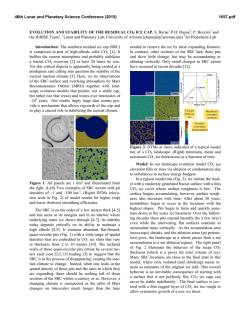


© Copyright 2026