
Land Misallocation and Productivity
Land Misallocation and Productivity†
Diego Restuccia
University of Toronto∗
Ra¨
ul Santaeul`alia-Llopis
Washington University in St. Louis∗∗
Universitat de Val`encia
February 2015
Abstract
Using detailed household-farm level data from Malawi, we measure real farm total factor productivity (TFP) controlling for a wide array of factor inputs, land quality, and transitory shocks.
The distribution of farm TFP has substantial dispersion but factor inputs are roughly evenly
spread among farmers. The striking fact is that operated land size and capital are essentially
unrelated to farm TFP implying a strong negative effect on agricultural productivity. A reallocation of factors to their efficient use among existing farmers would increase agricultural
productivity by a factor of 3.6-fold. We relate factor misallocation to severely restricted land
markets as the vast majority of land is without a title and a very small portion of operated
land is rented in. The gains from reallocation are 2.6 times larger for farms with no marketed
land than for farms that operate marketed land.
Keywords: misallocation, land, productivity, agriculture, Malawi, micro data.
JEL codes: O1, O4.
†
For helpful comments we thank Nadege Azebaze, Chang-Tai Hsieh, Leandro M. de Magalhaes, Matthias
Doepke, Pascaline Dupas, Chad Jones, Pete Klenow, Evelyn Korn, Rody Manuelli, Nancy Qian, Jos´e-V´ıctor
R´ıos-Rull, Paul Romer, Nancy Stokey, Kei-Mu Yi, and seminar participants at Edinburgh, ENSAI, Stanford
Institute for Theoretical Economics, SED Annual Meetings, NBER Summer Institute, University of Toronto,
IMF Workshop on Macroeconomic Policy and Income Inequality, CIDE Mexico, Queen’s University, University
of Marburg, Universitat d’Alacant, CEMFI, RIDGE workshop, and Wilfried Laurier University. All remaining
errors are our own. Restuccia gratefully acknowledges the financial support from the Social Sciences and
Humanities Research Council of Canada. Santaeul`alia-Llopis gratefully thanks the Weidenbaum Center on the
Economy, Government, and Public Policy for financial support.
∗
150 St. George Street, Toronto, ON M5S 3G7, Canada. E-mail: [email protected].
∗∗
Seigle Hall 339, Campus Box 1208, St. Louis, MO, 63130-4899, USA. E-mail: [email protected].
1
1
Introduction
A fundamental question in the field of economic growth and development is why some countries
are rich and others poor. The literature has offered many useful perspectives but in this paper
we build on two. First, agriculture is important in accounting for productivity differences
between rich and poor countries. This is because poor countries are much less productive in
agriculture and allocate most of their labor to this sector than rich countries. Moreover, low
productivity in agriculture together with a subsistence constraint for food explains the large
fraction of employment in agriculture in poor countries. As a result, the key question is why
agricultural labor productivity is so low in poor countries.1 Second, (mis)allocation of factors
of production across heterogeneous production units is important in explaining differences in
measured productivity across countries.2 In particular, Adamopoulos and Restuccia (2014a)
emphasize that misallocation in the agricultural sector in poor countries, specifically policies
and institutions that affect land allocations and farm size, may explain their low agricultural
productivity. In this paper, we use detailed household-farm level data from Malawi to measure
real farm total factor productivity (TFP) controlling for a wide array of factor inputs, land
quality, and transitory shocks. We show that operated land size and capital are essentially
unrelated to farm TFP which provides direct and comprehensive evidence of misallocation.
Factor misallocation has a substantial negative effect on agricultural productivity. Importantly,
we provide evidence that the bulk of productivity losses are associated with restricted land
markets.
Malawi represents an interesting case to study for several reasons. First, Malawi is an extremely poor country in Africa. According to international comparable measures of output,
Malawi GDP per capita in 1990 is around 1/35 that of the United States. Most of this difference is due to low labor productivity. Second, as with most poor countries, labor productivity
in the agricultural sector in Malawi is much lower than in the aggregate. For instance, agricul1
2
See, for instance, Restuccia et al. (2008).
See Banerjee and Duflo (2005), Restuccia and Rogerson (2008), Hsieh and Klenow (2009), among others.
2
tural GDP per worker relative to that of the United States in 1990 is 1/104 whereas relative
aggregate GDP per worker in the same year is 1/39.3 The distinction between aggregate productivity and agricultural productivity is important since in Malawi most of the employment
is in the agricultural sector. The share of employment in agriculture in Malawi in 1990 is 65%
whereas this share is only 2.5% in the United States. Third, the land market in Malawi is
largely underdeveloped. Most of the land in Malawi is customary and without a title. In our
sample, more than 83% of household farms do not operate any marketed land (either purchased
or rented-in). For these households land is typically granted by local leaders, transmitted by
inheritance, or received as bride price. Finally, the land distribution in Malawi is fairly concentrated in extremely small operational scales, with more than 70 percent of all households
operating less than 2 acres of land (less than 1 hectare). Following, Adamopoulos and Restuccia
(2014a), we argue that a plausible explanation to low productivity in agriculture in Malawi is
the misallocation of factors associated with frictions, policies and institutions that affect the
distribution of operated land.
We assess the quantitative importance of factor misallocation using detailed household-farm
micro data from Malawi. A key element of the analysis is the measure of real farm TFP which
requires detailed information on outputs, inputs, and other factors. The data is the 2010/11
Integrated Survey of Agriculture (ISA) for Malawi collected by the World Bank and consists of a
large nationally-representative sample of more than 12 thousand households. Using the detailed
micro data we measure real farm productivity controlling for a wide array of factor inputs, land
quality, and transitory shocks. Even though there is substantial dispersion in our measure of
farm TFP, factors of production are roughly evenly spread among farmers. The striking fact
is that operated land size and capital are essentially unrelated to farm productivity. These
patterns imply that the marginal products of capital and land are strongly positively related
with farm TFP which, under a standard framework of farm size constitutes evidence of factor
misallocation.
3
See, for instance, Restuccia et al. (2008) and Adamopoulos and Restuccia (2014a).
3
To assess the role of misallocation on agricultural productivity in Malawi, we consider as a
benchmark the efficient allocation of factors across existing household-farms in the data, taking
as given the total amounts of land and capital. We calculate the aggregate output loss as the
ratio of actual to efficient output, where the efficient output is the aggregate agricultural output
resulting from the efficient allocation of capital and land across farms. Since the total amounts
of capital, land, and number of farmers are kept the same under the efficient allocation, the
output loss is equivalent to a TFP loss. Our main finding is that the output loss is 0.28 in the
full sample. That is, if capital and land are reallocated across farms in Malawi to their efficient
uses, agricultural productivity would increase by a factor of 3.6-fold. This large productivity
impact of misallocation would unravel a substantial process of structural change with broader
implications for aggregate outcomes. For instance, in the context of a simple two-sector model,
the increase in agricultural TFP would reduce the share of employment in agriculture from 65
percent to 4 percent, and it would increase agricultural labor productivity and average farm size
by a factor of 16.2-fold. These effects would be even larger in a more sophisticated model that
includes ability selection across sectors such as that in Lagakos and Waugh (2013), endogenous
investment by farmers as in Goldstein and Udry (2008), endogenous human and physical capital
accumulation, among other well-studied channels in the literature.
In order to put our evidence of factor misallocation in Malawi and its large negative impact
on agricultural productivity in perspective relative to the existing literature, we note that
our evidence is closely linked to the seminal work of Hsieh and Klenow (2009) for the the
manufacturing sector in China and India. Our analysis contributes to this work by providing
evidence of misallocation in agriculture in a very poor country that is less subject to concerns
of measurement and specification errors that has casted doubt on the extent of misallocation in
poor countries. The evidence of misallocation we provide is strong because: (a) it is easier to
measure output and productivity in agriculture than in other sectors, essentially outputs and
most inputs are easily measured in quantities, (b) the micro data provides precise measures
of quantity and quality of inputs as well as transitory shocks, and there are very few missing
4
observations, making the analysis less subject to measurement and specification errors, and (c)
the large sample size and prevalence of maize production allow us to corroborate the extent of
misallocation for farms that produce essentially the same crop within narrow geographic and
other relevant characteristics. For these reasons we argue that, to the best of our knowledge,
our analysis constitutes the most direct and comprehensive evidence of misallocation in a poor
country.
A limitation of the empirical literature on factor misallocation is the weak link between misallocation and the policies and institutions that cause it. While this limitation has inspired
a promising quantitative literature studying specific policies and institutions, the findings are
yet elusive in explaining the bulk of TFP differences across countries.4 In this context, another
important contribution of our paper is to provide a strong empirical connection between factor misallocation and the limited market for land, showing large productivity losses associated
with restricted land markets. The evidence comes from contrasting the output losses among
farmers that have no marketed land to those that operate marketed land. We also contrast
the difference in the output loss that arises from different forms of marketed land, such as land
purchased with or without a title and land rented formally or informally. Our findings are
striking. The output loss of farms that operate land that is not marketed is 0.24 (slightly larger
than the 0.28 output loss in the full sample). But for farms that operate some marketed land,
the output loss is cut by half to 0.51. The output loss for farms with all marketed land is 0.64.
To put it differently, the gains from reallocation are 2.6 times larger for farms with no marketed
land than for farms with only marketed land. Among farms with marketed land, we find that
the lowest output losses are for farms that operate land purchased with a title, with an average
output loss of 0.72. These results have important implications for the design of policies and
institutions to promote a better allocation of factors.
We find that misallocation has important implications for income inequality. Even though
the actual allocation of factors is evenly spread among heterogeneous farmers, we find that
4
See for instance the surveys in Restuccia and Rogerson (2013) and Hopenhayn (2014).
5
factor equalization is ineffective at equalizing incomes in Malawi, in addition to its negative
effect on agricultural productivity already discussed. Taking the actual allocation of factors as
endowments and decentralizing the efficient allocation via perfectly competitive rental markets,
we show that the income distribution associated with the efficient allocation features not only
much lower overall income inequality, but also that the largest gains are accrued by the poorest
farmers. For instance, whereas the ratio of actual income in the top to bottom quintile of the
productivity distribution is a factor of 34-fold, it is reduced to a factor of 4-fold in the efficient
allocation. Moreover, whereas the efficient to actual income ratio increases by a factor of 2-fold
for the top quintile of the productivity distribution, the increase is a factor of 24-fold for the
bottom quintile and 4-fold for the second quintile. Hence, the poorest farmers benefit the most
from the reorganization of operational scales. A market arrangement where operational scales
can deviate from land holdings substantially improves aggregate income, reduces poverty, and
alleviates income inequality relative to operational scales that favor factor equalization across
household farms.
Our paper relates to the broad literatures on misallocation and the role of agriculture in aggregate productivity discussed earlier. In addition, our paper is closely related to a set of
papers emphasizing misallocation of land as an important factor, for instance Adamopoulos
and Restuccia (2014a), Chen (2014), and Adamopoulos and Restuccia (2014b). Chen (2014)
extends a standard model of farm size by allowing for untitled land and studying the aggregate impact of differences in the extent of untitled land across countries. Adamopoulos and
Restuccia (2014b) study the misallocation and productivity impact of a specific land policy:
land reforms. We differ from these papers in studying land misallocation in an economy with a
severely restricted land market to assess the aggregate impact of factor misallocation. Our result on the aggregate impact of factor misallocation is several orders of magnitude larger than
previously found, suggesting an important role of imperfections in land markets for the low
productivity in poor countries. Our emphasis on the importance of land markets connects to
6
the literature in development studying the role of land rights for investment in agriculture.5 We
complement this literature by emphasizing the importance of land markets for the allocation
of factors across productive uses in the agricultural sector. Like Adamopoulos and Restuccia
(2014b), our paper uses micro data to study macro development, an approach that relates to a
growing literature in macroeconomics.6
The paper proceeds as follows. In the next section, we describe the important elements of
the micro data for our analysis and in Section 3 we report the main facts from the data
in Malawi. In section 4 we assess the productivity impact of misallocation by comparing
aggregate agricultural output in the actual data to the hypothetical efficient allocation of factors.
We discuss output losses across geographical areas, traditional authority, language, specific
skills, as well as across the extent of access to marketed land. We also report some robustness
exercises. Section 5 explores the income inequality implications of the reallocation of factors to
the efficient allocation. In section 6 we discuss the broader implications of reallocation in the
context of a two-sector model. We conclude in Section 7. An on-line appendix is available at:
https://www.dropbox.com/s/je5wv90trv2nmq3/RS_Online_Appendix.pdf?dl=0.
2
Data
We use a new and unique household-level data set collected by the World Bank, the Malawi
Integrated Survey on Agriculture (ISA) 2010/11. The survey is comprehensive in the collection
of the entire agricultural production (i.e., physical amounts by crop and plot) and the full set
of inputs used in all agricultural activities at the plot level, all collected by a new and enlarged
agricultural module that distinguish ISA from previous Living Standards Measurement Study
(LSMS) surveys. The data are nationally-representative with a sampling frame based on the
5
See for instance Goldstein and Udry (2008) and the references therein.
See for instance Hsieh and Klenow (2009); Buera et al. (2014); Gollin et al. (2014); and de Magalhaes and
Santaeul`
alia-Llopis (2014a), among others.
6
7
Census and an original sample that includes 12,271 households (and 56,397 individuals) of
which 81% live in rural areas.7
The survey provides information on household-farm characteristics over the entire year and
we focus our attention to agricultural activities related to the rainy season. The detail on
household-farm agricultural production is excruciating. Information on agricultural production
is provided by each and all crops produced by the household. This is an economy largely based
on maize production that uses 80% of the total land. The total quantity of crop harvested
per crop and by each household is available per plot. We then value agricultural production
using median at-the-gate prices per region. In crop production, each household potentially
uses different quantities of intermediate inputs such as fertilizers, herbicides, pesticides and
seeds. This information is also provided by plot. We also apply common median prices to value
these intermediate inputs. As a result, our benchmark measure of household-farm output is a
common-price measure of value added constructed as the value of agricultural production (of
all crops) minus the costs of the full set of intermediate inputs.8
We measure household land as the sum of the size of each cultivated household plot. This
includes rented-in land, which consists of 12.5% of all cultivated land. On average, household
farms cultivate 1.8 plots.9 Plot size is recorded in acres using GPS (with precision of 1%
of an acre) for 98% of plots (for the remaining 2% of plots, size is estimated). Further, the
data contains very detailed information on the quality of land for each plot used in every
household. There are 11 dimensions of land quality reported: elevation, slope, erosion, soil
quality, nutrient availability, nutrient retention capacity, rooting conditions, oxygen availability
7
The Malawi ISA is part of a new initiative funded by the Bill & Melinda Gates Foundation (BMGF) and
led by the Living Standards Measurement Study (LSMS) Team in the Development Research Group (DECRG)
of the World Bank. We provide further details on the Malawi ISA and the construction of agricultural output
and its factor inputs in the Appendix A. See also de Magalhaes and Santaeul`alia-Llopis (2014b) for a broader
analysis of cross-sectional facts of ISA data for different Sub-Saharan countries.
8
We discuss in Section 4 the implications of subsidized input prices, i.e., purchases of fertilizers done by
redeeming coupons provided by the Malawi Input Subsidy Program for our measure of productivity and our
results on the productivity effects of misallocation.
9
Land is the largest household asset representing 46% of household total wealth. House structure is 27%,
livestock is 11%, agricultural equipment and structures (eg. tools and barns) is 3%, see de Magalhaes and
Santaeul`
alia-Llopis (2014b).
8
to roots, excess salts, topicality, and workability. This allows us to control for land quality to
measure household-farm productivity.
In terms of agricultural capital, we have information on both equipment and structures. Capital
equipment includes implements (hand hoe, slasher, axe, sprayer, panga knife, sickle, treadle
pump, watering can, and so on) and machinery (e.g. ox cart, ox plough, tractor, tractor
plough, ridger, cultivator, generator, motorized pump, grain mill, and so on), while capital
structures includes chicken houses, livestock kraals, poultry kraals, storage houses, granaries,
barns, pig sties, among others. To proxy for capital services after conditioning for its use in
agricultural activities, we aggregate across the capital items evaluated at the estimated current
selling price.10
In Malawi, a large proportion of the households members, beside the household head, contribute
to agricultural work. Household size is 4.6 with extended families in which several generations
live together in a single household. We use the survey definition of household members as
individuals that have lived in the household at least 9 months in the last 12 months. In terms
hours, data are collected at the plot level for each individual that participates in agriculture and
by agricultural activity (i.e., land preparation/planting, weeding/fertilizing, and harvesting).
Precisely, our data provides information of weeks, days per week, and hours per day employed
per plot, activity and individual. To compute household-farm hours we aggregate the hours of
all plots, activities and individuals. Further, the same information is provided for hired labor
and labor received in exchange (for free), but most household-farm hours consist of family hours.
We add hours by hired labor and free exchange of labor to our measure of total household hours.
Since our data comprises a single cross section of households for 2010-11, it is important to
control for temporary output shocks that may explain variation in output and hence produc10
This selling price for agricultural capital items, rarely available in previous LSMS data, helps capture
potential differences in the quality and depreciation of capital across farms. We provide robustness of our
results to alternative physical measures of agricultural capital such as asset indexes for agricultural equipment
and structures in Appendix B.2.2. We find that using these alternative indexes to proxy for agricultural capital
renders larger output losses and gains from reallocation relative to our baseline measure of capital.
9
tivity across households in the data. The single most important temporary shock for farmers
is weather. We use the annual precipitation which is total rainfall in millimetres (mm) in the
last 12 months. In further robustness exercises, we net household-productivity from additional
transitory shocks in the form of health, deaths or food security risks suffered by the household
in the last 12 months.
Geographic and institutional characteristics are also recorded for each household-farm. We use
several partitions of these characteristics to conduct robustness exercises. In particular, we use
geographical information on the region, districts, and enumeration area to which householdfarms belong and institutional characteristics such as the traditional authority (TA) governing
the household-farm or ethno-linguistic characteristics. TAs are relevant for our exercise as chiefs
appointed by TAs perform a variety of functions that include resolving issues related to land
and property.11
Finally, we note that the survey response is very high with little very few missing observations.
Conditioning on households that produce agricultural output and for which all factor inputs,
including the 11 dimensions on land quality, are available and further trimming about 1% of
the household-farm productivity distribution, our sample consists of 7,157 households.12
To summarize, the data allows us to obtain precise measures of real household-farm productiv11
Traditional Authorities are part of the administrative structure of Malawi. Any one district is only in one
region, any one TA is only in one district. Traditional authorities (and their sub-ordinate chiefs) are ’town
chiefs’ formally recognized under the Chiefs Act (1967) and receive a monetary honorarium by the government.
The Chiefs Act states that chieftaincies are hereditary and hierarchical, being the highest level in the TA or the
Paramount Chief (PC) and TAs cover the entire country. There can be several TAs within each ethno-linguistic
group. The sub-structure is such that below each TA there are Sub-TAs, Group Village Headmen (GVH), and
Village Headmen (VH). All villages have a VH, and several villages will be grouped under one GVH. These
chiefs perform a variety of functions: cultural affairs, administration and management of various sorts, oversight
of issues related to land and property, resolving disputes, an involvement in politics, and promoting economic
and social development. The TAs that we use in our reallocation exercise are the ones provided by Malawi ISA
2010/11 which are a subset of those used by the National Statistical Office to organize the data collection of
the Malawi Census. There are about 380 populated TAs and wards in the country with an average population
of just under 26,000 persons; TAs are found in rural areas, while urban-equivalent administrative wards are in
the four urban centers of Blantyre, Lilongwe, Mzuzu, and Zomba. District and local government authorities
may recognize additional TAs or sub-chiefs used in order to create reasonably sized administrative units within
large TAs.
12
See further details on the trimming strategy in Appendix B.1.
10
ity which is a key input in our assessment of factor misallocation in Malawi and its aggregate
productivity impact. Overall, ISA represents a substantial improvement with respect to previous LSMS questionnaires. The detailed information on quantity inputs and outputs reduces
substantially the possibility of measurement error and composition bias, making this dataset
ideal for our purpose of measuring productivity at the farm level, assessing the quantitative
extent of factor misallocation in the Malawian economy, and the extent to which productivity
losses due to misallocation are related to imperfections or frictions in the land market.
3
Facts
We use the micro data from ISA 2010/11 described in the previous section to emphasize the
following facts about the allocation of factors and productivity in the agricultural sector in
Malawi.
Fact 1: Operational Scale. The operational scale of farms is extremely small. For each
household, we compute the amount of land used for agricultural production regardless of the
land status (whether land is owned, rented, etc.). Hence, we focus on the operational scale of
the household-farm. We find that 78.3% of households operate less than 1 hectare (henceforth,
Ha.), 96.1% of households operate less than 2 Ha., and only 0.3% of households operate more
than 5 Ha., see the first column in Table 1. The average farm size is 0.83 Ha. To make a
comparison of operational scales in Malawi with other countries, we also report the distribution
of farm sizes from the World Census of Agriculture in Adamopoulos and Restuccia (2014a).
These data include all land used for agricultural production and corresponds to the year 1990.
Table 1 reports summary statistics. First, we note that despite the 20 years difference between
ISA 2010/11 and the Census 1990 the distribution of land across the two sources is very similar. Second, comparatively with other countries, the operational scale of farms in Malawi is
11
extremely small, ∼0.70-0.83 Ha., whereas average farm size is 187 Ha. in the United States
and 16.1 Ha. in Belgium. Belgium is a good reference for a developed country since the land
endowment (measured as land per capita) is similar to that of Malawi (land per capita is 0.56
Ha. in Malawi and 0.5 Ha. in Belgium, whereas land per capita is 1.51 Ha. in the United States).
Fact 2: Land Markets. The land market is largely underdeveloped in Malawi. We find
that the proportion of household-farms that do not operate any marketed land is 83.4%. These
are households that obtain their land granted by a village chief, inherited or as bride price.
The remaining 16.6% of households operate some land obtained from the market, either rented
or purchased, and the proportion of household-farms whose entire operated land was obtained
in the market is 10.4%. Disaggregating the main types of marketed land, we find that 3.0%
of household-farms rent-in land informally (e.g., land borrowed for free or moved in without
permission), 9.5% rent-in land formally (e.g., leaseholds, short-term rentals or farming as a
tenant), 1.8% purchase land without a title and 1.3% purchase land with a title.
Fact 3: Subsistence Consumption. We find that most farmers produce agricultural goods
for their own consumption and very little agricultural output is sold in the market. We illustrate this finding using some standard proxies for subsistence consumption in Figure 1. Figure
1, panel (a), reports the density of the share of food on nondurable expenditures. There is a
high degree of reliance on food in the household’s consumption budget. On average 65% of
household nondurables consist of food, with a median household consuming 72% of its nondurables expenditures in food.13 Figure 1, panel (b), reports a set of subsistence consumption
proxies against each percentile of the distribution of operated land. First, the food share of
consumption is rather inelastic with respect to land. Second, food security risk, defined as a
situation of not enough food to feed all household members in the last 12 months, is suffered
by 48% of households and while this risk tends to decline with land, land is not able to fully
13
We use deseasonalized and annualized consumption measures in de Magalhaes and Santaeul`alia-Llopis
(2014a).
12
hedge against it; more than 32% percent of households in the top 10% of the land distribution
still face some shortage of food. Third, the share of agricultural sales in total agricultural
production is on average 11% and this only raises to 19% for the households at the top 10%
of the land distribution. What the patterns in these figures show is that Malawi is essentially
characterized as a subsistence economy.
Fact 4: Land Quality. There are important differences in the land characteristics of farms.
For instance, Table 2 documents the heterogeneity in terrain roughness (elevation and slope).
For the full sample, more than 34 percent of land is high-altitude plains while around 20 percent
are low plateaus and 19 percent mid-altitude plateaus. These characteristics also differ by region
where the center region is mostly high-altitude plains whereas the south region is mostly low
plateaus. Figure 2, panel (a) and (b), further document these differences in elevation and slope
across farms and within regions. As a result of the heterogeneity in land characteristics, it is
important to control for land quality in our measure of productivity. To do so, we construct
an index of land quality as follows. Our benchmark land quality index is qi0 is constructed
by regressing log output in each farm on the full set of land quality dimensions described in
Section 2.14 Figure 3, panel (a), reports the distribution of the land quality index q across
households in the full sample and across regions. There are substantial variations in q across
households and across regions. In Table 3 we report the dispersion (variance of the log) of land
quality indexes versus the dispersion in the quantity of land across households in our data. The
main observation from Table 3 is that while there is variation in land quality across farmers,
the variation is not substantial relative to the variation in the quantity of land and the variation
in the amount of agricultural output. For instance, the variance of log quality relative to the
variance of log quantity of land is only 4.7 percent. Land quality variation is also low within
regions and within individual land characteristics. Our conclusion of a small quantitative role
of land quality for output differences across household farms is robust to variations in the index
14
We have also considered alternative land quality indexes for subsets of the land quality dimensions and with
different forms of land size and capital controls in Appendix A.2.
13
and to more flexible functional forms. We discuss these variations in Appendix A.2.
Fact 5: Rain Shocks. In Malawi, weather shocks, in particular rain, is the single most
important source of transitory shocks to agricultural production—we find that most cropland
is rain-fed and 84% of household-farms do not have any alternative irrigation system. Figure 3,
panel (b), reports the density of rain for the entire population of farmers and, separately, for
farmers within regions. We note what appear substantial differences across household-farms
and regions with median values for the Center and South region that fall below the range of
of the distribution of rain in the North region. To quantify the actual dispersion in rain we
report the variance of logs of rain in the bottom of Table 3 for our entire sample and regions.
We find that the dispersion of rain is very small compared to the dispersion in land size and
even smaller relative to output. In particular, the dispersion in annual precipitation is 5.2%
that of land size and 2.1% that of agricultural output. The small role of rain variation further
appears within regions, districts, and enumeration areas, as well as using alternative definitions
of precipitation measures, with mean cross-sectional variances that decline with the size of the
geographical area. In short, rain is not a substantial contributor to output variation across
farm households in Malawi.
Fact 6: Household-Farm Productivity. Using the micro data, we measure farm productivity and find that factors of production are strongly misallocated across farmers in Malawi.
For instance, we find that the amount of land and capital in farms is essentially uncorrelated
with farm productivity which is inconsistent with the efficient allocation of factors in any standard model of farm size. The implications of these patterns is that land productivity, which
is proportional to output per unit of land, and capital productivity, which is proportional to
output per unit of capital, are strongly dispersed across farms and increasing in farm productivity, whereas in an efficient allocation these measures of factor productivity should be roughly
equal across farmers. We measure farm productivity by exploiting the detailed micro data
14
where not only we obtain real measures of output and value added but also control for land
quality and transitory shocks such as rain as described previously. We measure farm-level total
factor productivity (TFP) si as the residual from the following farm-level production function
yi = si ζi k θk (qi li )θl where yi , ki , and li are output, capital, and land at the farm level in per
hour terms, ζi is a rain shock, qi is land quality, and θk,l are the input elasticities.15 We choose
θk = 0.36 and θl = 0.18 from the capital and land income shares in U.S. agriculture reported
in Valentinyi and Herrendorf (2008). Figure 4 documents the distribution of farm productivity
across all households in our sample. There are large differences in farm productivity across
households that remain even within regions. The dispersion in farm productivity compares in
magnitude to that of the variation in productivity (TFPQ) across plants in the manufacturing
sector in the United States, China, and India reported in Hsieh and Klenow (2009), see the
summary statistics reported in Table 4. Table 5 reports the variance decomposition of farm
output per hour using the assumed production function above. We note that farm productivity
si and to a lesser extent inputs of capital and land are the key determinants of output variation
across farm households in Malawi, with rain and land quality playing a quantitatively minor
role.
What is important to keep in mind in looking at farm-level observations is that in a standard
model of farm size such as that in Adamopoulos and Restuccia (2014a), the efficient allocation
of factors is such that more productive farmers would operate larger farms (operate more land),
operate more capital, and produce more output. Essentially, an efficient allocation of factors
across heterogeneous farmers is that factors are allocated to the most productive uses, until
the marginal product of each factor is equalized across farmers. Figures 5 and 6 report several
variables of interest across farms by farm-level TFP si . The patterns are striking. The data
show that the actual allocations of land and capital in farms are unrelated to farm productivity.
Figure 5, panel (a), shows the amount of land in each farm by farm productivity using our
15
Our analysis uses measures of output, capital, and land per hour as our emphasis is on the allocation of
land and capital across household farms. We note, however, that hours in farms are uncorrelated with farm
TFP and, as a result, our characterization and analysis is unaffected by treating hours as an explicit input in
the farm production function.
15
benchmark measure of productivity that adjusts for rain and quality as described previously.
Land in farms is essentially uncorrelated to farm TFP, the correlation between land size and
productivity is 0.05. Figure 5, panel (b), documents the relationship between the amount of
capital in farms by farm productivity. Capital and productivity across farms are essentially
unrelated, the correlation between the two variables is -0.01. Figure 5, panel (c), shows that
the capital to land ratio is essentially unrelated to farm productivity, with a correlation between
these variables of -0.03.
Whereas in an efficient allocation more productive farms should command more capital and land
to the point of equalizing the marginal products of these factors, the lack of positive relationship
between land and capital suggests that the marginal product of these factors are not equated
across farms indicating misallocation. Figure 6, panels (a) and (b), show that the marginal
product of land (proportional to the yield or output per unit of land) and capital (proportional
to output per unit of capital) are strongly positively correlated with farm productivity. The
correlation between these measures of factor productivity and farm TFP are .77 and .76 in each
case.
To summarize, the actual allocation of land across farmers in Malawi is unrelated to farm
productivity which is consistent with our characterization of the land market where the amount
of land in farms is more closely related to inheritance norms and redistribution and access to
land is severely restricted in rental and sale markets so more productive farmers cannot grow
their size. Capital is also unrelated to farm productivity with the capital to land ratio being
roughly constant across farm productivity. Our interpretation of this finding is that restrictions
to land markets are also affecting capital allocations echoing de Soto (2000) findings that land
market restrictions and insecure property rights of farmers limit the ability to raise capital
for agricultural production.16 These findings constitute strong evidence of land and capital
misallocation across farmers in Malawi. We emphasize that since farm size and productivity
16
We find further direct evidence of the relationship between land markets and access to credit in our micro
data for Malawi, see Appendix C.2 for a discussion. See also the related discussion in Besley and Ghatak (2009).
16
are essentially unrelated in Malawi, it is misleading to characterize farm level observations
and diagnose policy recommendations based on the more common measure of farm size. This
echoes the work of Restuccia and Rogerson (2008) and Adamopoulos and Restuccia (2014a) in
emphasizing the role of policies and institutions driving a wedge between size and productivity
at the establishment level in developing countries.
4
Quantitative Analysis
How important is land and capital misallocation for aggregate productivity? We assess the
quantitative impact of factor misallocation on agricultural productivity in Malawi. We do
so without imposing any additional structure other than the farm-level production function
assumed in the construction of our measure of household-farm productivity. As a benchmark
for comparison, we solve for the efficient allocation of factors across farms given the total
amounts of capital and land. We compare the implications of the efficient allocations versus
the actual allocations on aggregate output and productivity in agriculture.
More specifically, we solve for the efficient allocation of capital and land across a fixed set of
heterogeneous farmers si . A planner chooses the allocation of capital and land across a given
set of farmers with productivity si to maximize agricultural output given fixed total amounts
of capital K and land L. The planner solves the following problem:
Y e = max
X
{ki ,li }
si (kiα li1−α )γ ,
i
subject to
K=
X
ki ,
L=
i
X
li .
i
The efficient allocation equates marginal products of capital and land across farms and has
1/(1−γ)
a simple form. Letting zi ≡ si
, the efficient allocations are given by simple shares of a
17
measure of productivity (zi /
P
zi ) of capital and land:
zi
kie = P K,
zi
zi
lie = P L.
zi
We note for further reference, that substituting the efficient allocation of capital an land into the
definition of aggregate agricultural output renders a simple constant returns to scale aggregate
production function for agriculture on capital, land, and agricultural farmers given by
Y e = ZNa1−γ [K α L1−α ]γ ,
(1)
P
where Z = ( zi g(zi ))1−γ is total factor productivity as the average productivity of farmers and
Na is the number of farms. We choose α and γ consistent with the production function used in
our measure of farm-level productivity so that αγ = 0.36 and (1 − α)γ = 0.18 as the capital and
land income shares in the U.S. economy reported in Valentinyi and Herrendorf (2008). This
implies γ = 0.54.17 The total amount of capital K and land L are the total amounts of capital
and land across the farmers in the data. Farm level productivity si ’s are given by our measure
of farm TFP from data as described previously. Before we move on to document the aggregate
impact of misallocation, we illustrate the extent of factor misallocation in Figure 7, where we
contrast the actual allocation of land and capital and the associated factor productivity by farm
TFP against the efficient allocation of factors and the associated factor productivities across
farms. In the efficient allocation, operational scales of land and capital are strongly increasing in
farm productivity so that factor productivity is constant across farms. The efficient allocation
contrasts sharply with the actual allocation in Malawi.
17
We use factor income shares from a developed economy as estimates of the elasticities in the production
function since variation in the corresponding measures in a poor country are likely reflecting frictions or distortions in factor markets. We evaluate the robustness of our results using different capital and land shares in the
Appendix F. Using the micro data we construct alternative capital and labor shares rendering similar aggregate
results. The main difference is that the land share in Malawi would be larger and hence implies larger effects of
land-only redistribution.
18
4.1
Results on the Output Loss
To summarize the impact of misallocation on productivity, in what follows we report the aggregate output loss defined as
P a
Ya
yi
=
,
e
Y
Ye
γ
where Y a is actual agricultural output aggregated from farm-level output using yi = si kiα li1−α ,
where k and l are actual allocations and; and Y e is efficient aggregate agricultural output as
defined previously. Because the efficient allocation takes as given the total amounts of capital,
land, and the number of farmers observed in the data, the output loss is also a TFP loss.18
Table 6, panel (a), reports the main results. For the full sample in the entire Malawi, the output
loss is 0.28, that is actual agricultural output is 28 percent of that of efficient agricultural output
at the aggregate level. We can also express the results in terms of the gains from reallocation
from the actual distribution of factors to the efficient, which is the inverse of the output loss.
If capital and land were reallocated efficiently in Malawi to maximize agricultural output,
output and hence productivity would increase by a 3.6-fold factor. This is a very large increase
in productivity as a result of a reduction in misallocation, at least compared to the results
in the misallocation literature when evaluating specific policies which has found increases on
the order of 5 to 30 percent. Even when eliminating all wedges in manufacturing in China and
India in Hsieh and Klenow (2009), the increases range between 100-160 percent. Given that the
real productivity dispersion across farms in Malawi is not much larger than the productivity
dispersion of manufacturing plants reported in Hsieh and Klenow (2009), what this result
suggests is that the actual allocation of resources in Malawi is much more distorted than that
of those other countries or to put it differently that factors are more severely misallocated in
Malawi.19 Because we have a large sample, our mean output loss is tightly estimated. In Table
18
The computation of actual output at the farm level abstracts from rain and land quality as it is the case in
the efficient allocation. We also emphasize that the empirical measure of farm productivity si is purged of rain
and land quality effects as described in Appendix A.
19
Note that a more direct comparison with the analysis of Hsieh and Klenow (2009) for the case of India
and China would be to report dispersion in log revenue productivity (TFPR). However, unlike for the case of
19
6, panel (a), we also report the 5 and 95 percentiles of Bootstrap estimates, which provide a
narrow interval between 0.25 and 0.32 for the aggregate output loss.20
We also report the output loss for narrower definitions of geographical areas and institutions
such as language classifications. Table 6, panel (b), reports these results. In the fist column, we
report the output loss for the average of regions (i.e., output loss of reallocating factors within
a region for each region and then averaged across regions), for the average across districts
(a narrower geographical definition than region), for the average across enumeration areas.
Enumeration areas are a survey-specific geographical description and is the narrower definition
available. Each enumeration area amounts to about 16 households in the data, which given
the average land holdings amounts to about 30 acres of geographically connected land. The
table reports results by Traditional Authority (TA) and language. Columns 2 to 4 report the
Median, Min, and Max in each case.
What is striking about the numbers in Table 6, panel (b), is that the gains from reallocation
are large in all cases, even within narrowly defined geographical areas, traditional authority
and language. In particular, reallocating capital and land within a region generates output
losses of the same magnitude as in the aggregate (mean output loss of 0.29).21 Similarly, within
districts, the average output loss is 0.34, but the output losses can be as large as 0.14 and the
lowest 0.48. Even for the narrowest geographical definition, enumeration areas, just reallocating
factors within 16 households, average output losses are 0.60 and can be as large as 0.09 in some
areas. Considering reallocation within enumeration areas also serves as a further check on the
relevance of land quality since within such a narrow geographical definition it is unlikely that
manufacturing firms, most of the production of farms in Malawi is not sold in markets and hence revenue of farms
would have to be imputed. More importantly, the micro data allow us to directly measure real productivity
across farms and hence assess the aggregate productivity implications without the need to characterize the
associated market wedges.
20
We also report the output loss when the dispersion in factor inputs is reduced across farm productivity
types, see Appendix B.2.3. In the more conservative case where all the dispersion within productivity groups
is eliminated, the output loss is still substantial .40 (versus .28 in the baseline) which implies a substantial
reallocation gain of 2.5-fold.
21
The idea is that narrower geographic definitions provide additional land quality control, see Larson et al.
(2014) for a similar strategy.
20
land quality plays much if any role. We also report the distribution of output losses in each
enumeration area in the survey in Figure 8. The output loss within traditional authorities is
0.32 in average, with the largest 0.18 and median 0.29. Within languages, the average output
loss is 0.30, the largest 0.17 and median 0.26.
4.2
The Role of Land Markets
We have found strong evidence that capital and land are severely misallocated in the agricultural
sector in Malawi. We connect this misallocation to the limited market for land in Malawi. Even
though the amount of operated land that is rented in or purchased is relatively small in our
data, we assess the output loss across farms that differ in the extent of marketed land in their
operation as further evidence of the connection of misallocation to land markets.
Table 7 reports the aggregate output loss for farms that operate with no marketed land, with
some marketed land as either rented in or purchased, and with only marketed land. The output
loss is much higher for those farms with no marketed land than with some marketed land. For
instance, the output loss for those farms with no marketed land, which comprises 83 percent of
the sample of household farms, is 0.24, slightly larger than the 0.28 output loss for the entire
sample. But for farms with some marketed land, which comprises the remaining 17 percent of
the sample farms, the output loss is 0.51. The striking finding is that the output loss of factor
misallocation is reduced by more than half when farms have access to some marketed land.
The output loss is even smaller among the set of farmers whose all their operated land is
either rented in or purchased. These farmers comprise 10 percent of the sample and have an
output loss of 0.64 versus 0.24 for farmers with no marketed land. That is, the gains from
reallocation are 2.6 times larger for farms with no marketed land than for farms that operate
only marketed land. Table 7 also decomposes the output losses among farmers by the type
of operated marketed land: (a) rented-in informally, for example land borrowed for free or
21
moved-in without permission; (b) rented-in formally such as leaseholds, short-term rentals or
farming as tenant; (c) purchased as untitled; and (d) purchased as titled. The vast majority of
farmers with some marketed land are formally renting-in, 9.5 percent of the sample out of the
17 percent with some marketed land. The output loss is fairly similar for farmers operating land
rented-in formally or informally, an output loss of roughly 0.58 for both. The lowest output
loss is recorded for farms with operated land that was purchased with a title, 0.72 versus 0.24
for farms with no marketed land. Interestingly, farmers with purchased land without a title
record a fairly large output loss, 0.20, somewhat larger than the output loss for farmers without
marketed land of 0.24. We note however that the sample of farms with purchased land is fairly
limited, only 3.1 percent of the sample: 1.8 percent of farms with purchased untitled land and
1.3 percent of farms with purchased titled land.
It is interesting to note that farms with and without marketed land differ along many dimensions, which we report in detail in the Appendix C, further asserting the importance of land
markets for farm operation. For instance, on average farms with some marketed land are more
productive than farms with no marked land. But greater access to land markets means that
farmers with marketed land command more inputs and produce more output but, as a result
of greater input use, capital and land productivity does not rise as much from farmers with no
marketed land. Further, we find that access to land markets is related with access to other markets (e.g., credit) and with other indicators of economic development. Farmers with marked
land are substantially more educated than farmers with no marketed land, women in these
farms are more empowered in terms of labor force participation and market wages, more of
these farmers are migrants, a fewer proportion live in rural areas, and a larger proportion of
these farmers invest in intermediate inputs and technology adoption.
22
4.3
Further Robustness Results
We conduct further robustness results to human capital and specific skills, transitory health
and other shocks, specific type of crops, and distortions to intermediate input use.
Human Capital and Specific Skills Table 8 reports robustness results with respect to
human capital and specific terrain skills. In each case, we perform the efficient reallocation
exercise discussed earlier but within each education and skill type. With respect to schooling
levels of the household head, the output losses are large at all schooling levels and roughly
constant across the human capital spectrum. For no schooling farmers the output loss is 0.31
and between 0.26 to 0.28 for farmers with primary and more than primary schooling. Output
losses may also be related to specific skills such as how to operate farms in different terrain
roughness. Similarly to our findings for human capital, the output losses are large even within
specific terrain roughness, 0.27 for high altitude plains and 0.36 for mid-altitude mountains.
Other Transitory Output Variation Table 9 reports the output losses associated with a
measure of farmer productivity that further adjusts for transitory health and other shocks. We
regress our benchmark measure of farm productivity on a set of controls for transitory shocks
which includes health and death shocks, food security risk, marital status, distance to markets
and the availability of other income sources. In each case, we use the residual from each of
these regressions as the new measure of farm productivity. Using these alternative measures of
productivity, we perform the efficient reallocation exercise discussed earlier. Output losses are
large in all cases, from 0.28 in the benchmark specification to 0.27 when using all controls.
Crop Type Production In our sample, close to 80% of land is devoted to maize production,
see also FAO (2013).22 Since optimal farm operational scale may differ across crop types, we
22
Maize, cassava, and potatoes are the main crops produced in Malawi in terms of volume with roughly equal
amount in tonnes, but it is maize that accumulates the vast majority of cropland. The importance of maize
23
investigate whether the output losses are different across farms producing different crops. Since
most farms produce both maize and non-maize crops, we consider reallocation among farms
that produce mostly maize and those farms that produce mostly non-maize. We report the
results in Table 10 where the first column is the output losses in the nationwide benchmark,
the next two columns are farms that produce mostly maize (whether the maize share is positive
or above the median of all farms), and the last two columns for those farms that produce
mostly non-maize (wether the non-maize share is positive or above the median). The output
loss among farms that produce maize is somewhat smaller (0.37 for farms with maize production
above the median versus 0.28 in the benchmark), which implies that the farms with non-maize
production have output losses that are larger (0.24 for farms that produce non-maize above the
median versus 0.28 in the benchmark). We conclude that crop composition and the dependence
of maize production in Malawi are not driving our main output-loss results.
Distortions to Intermediate Inputs Our main results are derived with a measure of farm
productivity that is constructed from value added output in each farm. As discussed earlier,
this measure of valued added is constructed using common agricultural output prices and common intermediate input prices so as to obtain a real measure of farm productivity that is devoid
of potential idiosyncratic price distortions in the economy. This is relevant in Malawi because
intermediate inputs are subsidized via the “Malawi Input Subsidy Program” and the basic allocation of the subsidies is based on income of the farmer, with poorer farmers receiving higher
subsidies. We assess the potential bias in our farm-productivity calculations if instead we construct farm productivity using actual expenditures on intermediate inputs by each farmer. If
poorer farmers are less productive than richer farmers but receive more subsidies to intermediate
inputs as it is the case in the data, using actual expenditures in intermediate inputs biases the
dispersion in farm productivity down, making less productive farmers appear more productive
than what they are. Figure 9, panel (a), documents that less productive farmers (which are also
further appears in terms of the household diet in Malawi where about 50% the average daily calorie intake
is obtained from maize, 8.4% from potatoes, and 5.8% from cassava, see FAO (2013) and de Magalhaes and
Santaeul`
alia-Llopis (2014a).
24
poor farmers) receive a subsidy that is more than 60 percent their output while more productive
farmers (richer farmers) receive a subsidy that is less than 10 percent their output. This implies
that a measure of productivity that uses actual expenditures in intermediate inputs instead of
the actual quantities of intermediate inputs substantially underestimates productivity dispersion across farms. This is illustrated in Figure 9, panel (b), where farm productivity and the
marginal product of land are reported for our baseline measure of farm productivity (that uses a
quantity measure of intermediate inputs) and a measure of productivity that uses expenditures.
The variance of the log productivity falls from 1.44 in our baseline measure of productivity to
0.85 using actual expenditures in intermediate inputs (a reduction in productivity dispersion
of more than 40 percent). The output loss associated with this biased measure of productivity
is 0.33, although still substantial, is 17 percent smaller than the output loss of 0.28 associated
with our baseline measure of farm productivity. This analysis also illustrates the importance of
the implementation of policies which in this case even well-intended policies further contribute
to distorting factor inputs.
5
Inequality Implications
Unlike the actual distribution of factors in the Malawian economy which is fairly flat across
farmers with different productivity, the efficient allocation implies a substantial increase in the
dispersion of operational scales, both in terms of the distribution of capital and land across
farmers. This massive redistribution of factors across farmers may lead to concerns over distributional implications, specially since the actual allocation of factors reflects policy choices and
institutional features in place partially to alleviate poverty and distributional concerns.
In this section, we study the distributional implications of redistributing operational scales
towards the efficient allocation. Table 11 reports the actual and efficient distribution of factors
across farmers by productivity and Table 12 reports actual and efficient output and income.
25
As discussed previously, whereas the actual distribution of land across farm TFP is fairly
flat, with most farms operating less than 2 acres of land, the efficient distribution implies
that the top quintile of farm TFP operates on average almost 6 acres and 97 percent of the
land whereas the lowest quintile only operates less than a percent of the land. This implies
a substantial redistribution of factors and operational scales to achieve the higher levels of
aggregate productivity. But it is important to emphasize that despite relative equalization
of factor inputs across farmers, the actual distribution of income is widely dispersed, in fact
as dispersed as the distribution of productivity. For instance, taking agricultural output as a
measure of farm income, the ratio of top to bottom quintile of income is a factor of 34-fold
even though the ratio of capital and land factors is within a factor of 1 to 2-fold. To put
it differently, equalizing access to land across households does not necessarily translate into
income equalization as these farmers differ substantially in their productivity of working the
farm.
To gauge the income effects of factor redistribution we pursue the following counterfactual. We
consider the actual distribution of factors as endowments and allow the efficient allocation of
factors to be achieved via perfectly competitive rental markets for capital and land, that is, with
perfect markets a decentralized competitive allocation corresponds to the efficient allocation.
Given the competitive rental rates of capital and land in this decentralized solution, we compute
the income associated with the efficient allocation as:
endowment income = rk (k a − k e ) + rl (la − le ) + y e ,
where (k a , la ) are the actual allocation of capital and land which we take as endowment and
(k e , le ) are the efficient allocations, rk and rl are the prices that support the efficient allocation
as a competitive equilibrium, and y e is efficient output. Table 12 reports the results for this
measure of endowment income and compare the income inequality to that of the actual income,
which we assume is approximated by actual output y a .
26
Not only farmers in the lower end of the productivity (and income) distribution benefit the
most from the increase in the average yield and aggregate agricultural output, but also overall
inequality declines. For instance, the overall variance of the log income decreases from 1.8 with
actual income to 1.2 to efficient income. More dramatic are the changes in income across the
richest and poorest households. Whereas the ratio of income between farmers in the top and
bottom quintiles is a factor of 34-fold in the actual allocation, this ratio is 3.4 in the efficient
allocation, that is income inequality among these farmers falls by a factor of 10-fold. Moreover,
the ratio of efficient to actual income increases for all household farms but this increase is much
larger for the households at the bottom of the productivity distribution, 23.7-fold for the first
quintile, 3.9-fold for the second quintile and only 2-fold for the top quintile.
Well-functioning rental markets for capital and land to achieve the efficient allocation of operational scales can lead to substantial increases in agricultural productivity as well as dramatic
reductions in inequality levels and poverty.
6
Two-Sector Implications
We assess the broader implications of reallocation by considering the effects of increased productivity in agriculture on the movement of factors across sectors. We argue that a TFP
increase of a 3.6-fold factor in the agricultural sector would produce a process of substantial
structural change in the Malawian economy. This reallocation would produce broad impacts
in the economy through well-known features such as the potential selection effects associated
with the movement of labor from agriculture to non-agriculture and dynamic investment effects
such as additional investments farmers would make to exploit increased farm size, capital and
human capital accumulation, among many others.
To provide a simple characterization of these broader implications of reallocation, we consider
27
an extension of the previous analysis to allow for a non-agricultural sector.23 Recall that the
aggregate production function for agriculture in the efficient allocation is given by equation (1).
To simplify the analysis, without much loss of generality, we abstract from capital by assuming
that α = 0. Hence, the aggregate production function in agriculture is given by:
Ya = ZLγ Na1−γ ,
where Na is the fraction of employment in agriculture and γ = 0.54. The non agricultural
production function is given by Yn = A(1 − Na ). We assume that preferences are such that
consumers not only have a minimum consumption of agricultural goods a
¯, but also this level is
a satiation point so per capita consumption of agricultural goods is given by a
¯ and any income
above the one required for this amount of agricultural consumption is spent on non-agricultural
goods.24 We continue to consider a benevolent social planner that chooses the allocation of
labor across sectors to maximize consumer’s welfare. Given our assumptions about preferences,
the solution to this allocation problem has a simple form and is given by:
1
a
¯ 1−γ
Na =
.
ZLγ
Note that the solution is such that an increase in productivity in the agricultural sector Z
reduces the share of employment in agriculture. In particular, the change in employment
in agriculture can be easily calculated using the above equation from the change in TFP in
agriculture raised to the power 1/(1 − γ). We report the results in Table 13. With γ = 0.54,
an increase in productivity of 3.6 implies a decrease in the employment share in agriculture of
16.2-fold. In other words, the share of employment in agriculture in Malawi would decrease
from the actual 65 percent to only 4 percent which is close to the average for rich countries, see
for instance Restuccia et al. (2008). This tremendous reallocation of labor from agriculture to
non-agriculture implies that average farm size would increase by a factor of 16.2-fold (recall that
23
For a more elaborate analysis of misallocation in agriculture in the context of a two-sector economy see
Adamopoulos and Restuccia (2014a).
24
See for instance Gollin et al. (2002) for a model with such preferences.
28
in our previous one-sector analysis of misallocation, by construction the gains in agricultural
productivity of moving to the efficient allocation involved no change in average farm size). It
is also easy to see that the increase in labor productivity in agriculture Ya /Na is given by a
factor of 16.2-fold, whereas agricultural output per unit of land or yield Ya /L remains the same.
This is because for the preferences we consider, the increase in productivity is exactly offset
by the decrease in agricultural labor so total agricultural output remains the same. Hence, for
our quantitative experiment, the entire increase in agricultural labor productivity is reflected
in an increase in average farm size and none in an increase in the yield. This implication is
roughly consistent with the findings from micro data across countries in Gollin et al. (2014)
where the large differences in agricultural labor productivity across countries is mostly reflected
in differences in average farm size (land per worker in agriculture).
We emphasize that the effects just described abstract from other potential sources of amplification. For instance, the potential role of selection into the ability of farmers that stay in
agriculture. This feature that has been found quantitatively important in amplifying the productivity increases in the agricultural sector. Lagakos and Waugh (2013) find that selection
can further increase productivity in the agricultural sector by a factor of more than 2-fold.
Also, complementary investments such as mechanization, improvements in land quality, or the
adoption of modern technologies could further increase productivity in the agricultural sector.
Overall, we find that the increase in agricultural productivity due to the more efficient allocation of factors can unravel a substantial process of structural change and productivity growth
in agriculture that can dramatically change the face of the Malawian economy.
7
Conclusions
We assessed the importance of factor misallocation for productivity in agriculture using detailed
household-level data from Malawi. The micro evidence indicated substantial misallocation of
29
capital and land in Malawi as factor inputs are essentially unrelated to farm TFP. Our results
provide direct and comprehensive evidence of misallocation in a poor country. The evidence is
strong as the unique data set allows for precise estimates of productivity at the household-farm
level.
To assess the aggregate productivity impact of misallocation, we considered as a benchmark the
efficient allocation of factors across a given set of heterogeneous farmers with farm-level TFP
measured in the data, holding the total amounts of capital and land. The main result is that
a reallocation of capital and land to their most efficient uses would increase productivity by a
factor of 3.6-fold. This large increase in agricultural productivity would unravel a substantial
process of structural change with broader implications for aggregate outcomes. Our analysis
also provided a strong empirical connection between factor misallocation and the limited market
for land, showing large productivity losses associated with restricted land markets. We found
that the gains from reallocation are 2.6 times larger for farms with no marketed land than
for farms with only marketed land. Our results emphasize the importance of land markets for
factor misallocation in agriculture that may explain the large productivity differences across
countries.
Our analysis takes the distribution of farmlands across productive farmers as given and asked
about the efficiency gains of reallocation. Understanding the institutional and policy elements
leading to the misallocation of land is useful in connecting the results with the design and
implementation of policy and development strategies. It may also be of interest to study the
dynamic implications of misallocation for productivity whereby a reduction in misallocation
encourages the more productive farmers to grow, utilize modern inputs (mechanization, chemical seeds, intermediate inputs), and invest in farm productivity, see for instance Restuccia and
Rogerson (2013) and Restuccia (2013). We leave these interesting and important extensions of
our analysis for future research.
30
References
Adamopoulos, T. and Restuccia, D. (2014a). The Size Distribution of Farms and International
Productivity Differences. American Economic Review, 104(6):1667–97.
Adamopoulos, T. and Restuccia, D. (2014b). Land Reform and Productivity: A Quantitative
Analysis with Micro Data.
Banerjee, A. V. and Duflo, E. (2005). Growth Theory through the Lens of Development
Economics. In Aghion, P. and Durlauf, S., editors, Handbook of Economic Growth, volume 1
of Handbook of Economic Growth, chapter 7, pages 473–552. Elsevier.
Besley, T. J. and Ghatak, M. (2009). The de Soto Effect. CEPR Discussion Papers 7259,
C.E.P.R. Discussion Papers.
Buera, F. J., Kaboski, J. P., and Shin, Y. (2014). Macro-perspective on Asset Grants Programs:
Occupational and Wealth Mobility. American Economic Review, 104(5):159–64.
Chen, C. (2014). Land Tenure, Occupational Choice and Agricultural Productivity,. Unpublished manuscript, University of Toronto.
de Magalhaes, L. and Santaeul`alia-Llopis, R. (2014a). Consumption and Expenditures in Poor
Countries: A Life With No Humps and Rural-Urban Insurance Traps to Growth. Unpublished
Manuscript Bristol University and Washington University in St. Louis.
de Magalhaes, L. and Santaeul`alia-Llopis, R. (2014b). The Consumption, Income and Wealth
of the Poorest: Cross-Sectional Facts of Rural and Urban Sub-Saharan Africa for Macroeconomists. Unpublished Manuscript Bristol University and Washington University in St.
Louis.
de Soto, H. (2000). The Mystery of Capital: Why Capitalism Triumphs in the West and Fails
Everywhere Else. Basic Books. New York.
FAO (2013). Malawi BEFS Country Brief. Technical report, Food and Agriculture Organization
of the United Nations.
Goldstein, M. and Udry, C. (2008). The profits of power: Land rights and agricultural investment in ghana. Journal of Political Economy, 116(6):981–1022.
Gollin, D., Lagakos, D., and Waugh, M. E. (2014). Agricultural Productivity Differences across
Countries. American Economic Review, 104(5):165–70.
Gollin, D., Parente, S., and Rogerson, R. (2002). The Role of Agriculture in Development.
American Economic Review, 92(2):160–164.
Hopenhayn, H. A. (2014). Firms, misallocation, and aggregate productivity: A review. Annual
Review of Economics, (0).
Hsieh, C.-T. and Klenow, P. J. (2009). Misallocation and Manufacturing TFP in China and
India. The Quarterly Journal of Economics, 124(4):1403–1448.
31
Lagakos, D. and Waugh, M. E. (2013). Selection, agriculture, and cross-country productivity
differences. The American Economic Review, 103(2):948–980.
Larson, D. F., Otsuka, K., Matsumoto, T., and Kilic, T. (2014). Should African rural development strategies depend on smallholder farms? An exploration of the inverse-productivity
hypothesis. Agricultural Economics, 45(3):355–367.
Restuccia, D. (2013). factor misallocation and development. The New Palgrave Dictionary
of Economics, Online Edition, Eds. Steven N. Durlauf and Lawrence E. Blume, Palgrave
Macmillan.
Restuccia, D. and Rogerson, R. (2008). Policy Distortions and Aggregate Productivity with
Heterogeneous Plants. Review of Economic Dynamics, 11(4):707–720.
Restuccia, D. and Rogerson, R. (2013). Misallocation and productivity. Review of Economic
Dynamics, 16(1):1–10.
Restuccia, D., Yang, D. T., and Zhu, X. (2008). Agriculture and aggregate productivity: A
quantitative cross-country analysis. Journal of Monetary Economics, 55(2):234–250.
Valentinyi, A. and Herrendorf, B. (2008). Measuring Factor Income Shares at the Sector Level.
Review of Economic Dynamics, 11(4):820–835.
32
Table 1: Size Distribution of Farms (% of Farms by Size)
ISA 2010/11
Malawi
Hectares (Ha):
≤ 1 Ha
1 − 2 Ha
2 − 5 Ha
5 − 10 Ha
10+ Ha
Average Farm Size (Ha)
78.3
17.8
3.7
0.2
0.0
0.83
World Census of Agriculture 1990
Malawi
Belgium
USA
77.7
17.3
5.0
0.0
0.0
0.7
14.6
8.5
15.5
14.8
46.6
16.1
–
–
10.6
7.5
81.9
187.0
Notes: The first column reports the land size distribution (in hectares) for household farms from the Malawi
2010/11 Integrated Survey of Agriculture (ISA). The other columns report statistics from the World Census of
Agriculture 1990 for Malawi, Belgium, and United States documented in Adamopoulos and Restuccia (2014a).
Table 2: Heterogeneity in Terrain Type, Malawi ISA 2010/11
Terrain Type:
Lowlands
Rugged Lowlands
Plains
Mid-altitude Plains
High-altitude Plains
Platforms (very low plateaus)
Low plateaus
Mid-altitude plateaus
Hills
Low Mountains
Mid-altitude Mountains
Full Sample
Terrain Elevation Slope
(%)
(meters)
(%)
By Region,
Terrain Type (%)
North Center South
1.03
.11
4.92
8.31
34.88
2.11
20.57
19.25
.62
3.38
4.82
132
106
86
474
873
401
727
1,218
381
769
1,314
5.98
16.23
1.71
1.76
2.34
6.19
6.46
6.55
16.83
15.98
16.59
.00
.00
.00
8.85
23.24
1.40
14.62
34.65
.29
3.90
13.05
.00
.00
.00
8.73
46.63
.23
7.56
32.09
.00
.26
4.50
2.16
.24
10.33
7.81
30.55
3.74
32.28
4.19
1.20
5.48
2.03
100.00
834
5.29
100.00
100.00
100.00
Notes: Terrain type can be broadly classified as a combination of elevation (in meters) and slope (in percent).
The first column reports the distribution of terrain type for our full sample and the second and third columns
report the average elevation and slope within each terrain type. The last three columns report the distribution
of terrain type (in percentage) by region.
33
Table 3: Dispersion of Output, Land Size, Land Quality, and Rain, Malawi ISA 2010/11
Full Sample
Within Geographic Areas
Regions Districts Enum. Area
Output, yi :
1.896
1.867
1.778
1.649
Land Size, li :
.749
.746
.719
.671
Land Quality:
B Index, qi
B Index Subitems:
Elevation
Slope (%)
Erosion
Soil Quality
Nutrient Avail.
Nutrient Ret. Cap.
Rooting Conditions
Oxygen Avail. to Roots
Excess Salts
Toxicity
Workability
.852
.833
.568
.147
.439
.657
.480
.608
.387
.329
.342
.097
.037
.027
.475
.349
.635
.496
.605
.402
.365
.372
.094
.045
.038
.474
.075
.453
.472
.514
.248
.180
.302
.105
.048
.033
.335
.001
.093
.427
.458
.023
.016
.029
.010
.004
.003
.033
Quality-Adjusted Land Size, qi li :
1.571
1.531
1.243
.808
Rain, ζi :
B Annual Precip. (mm)
B Precip. of Wettest Qrter (mm)
.039
.026
.025
.013
.014
.005
.001
.000
Notes: Output yi , land size (in acres) li , land quality index qi , quality-adjusted land size qi li , and rain ζi , are
continuous variables for which we use the variance of logs as a measure of dispersion. Subitems of land quality,
slope (in %) and elevation (in meters), are also continuous variables and we also report the variance of logs
as dispersion measure. The other subitems of land quality are categorical variables such as soil quality (with
categories 1 good, 2 fair, 3 poor), erosion (with categories 1 none, 2 low, 3 moderate, 4 high) and nutrient
availability, nutrient retention, rooting conditions, oxygen to roots, excess of salts, toxicity and workability that
take values from four categories (1 low constraint, 2 moderate constraint, 3 severe constraint and 4 very severe
constraint). For all categorial variables we use the proportion of non-mode values in the sample as measure of
dispersion. The construction of the land quality index qi is discussed in Section 3. For the last three columns
referring to within geographic areas, we report the averages across geographic area under consideration (e.g.,
the variance of output in the ’Regions’ column is the average across regions of the variance of output by region).
34
Table 4: Dispersion of Productivity across Farms and Manufacturing Plants
Statistic
SD
75-25
90-10
N
Farms
Malawi
USA
ISA 2010/11
1990
1.19
1.15(3.2)
2.38(10.8)
7,157
0.80
1.97
2.50
AR(2014)
Manufacturing Plants
USA
China India
1977
1998
1987
0.85
1.22
2.22
164,971
1.06
1.41
2.72
95,980
1.16
1.55
2.77
31,602
Notes: The first column reports statistics for the household-farm productivity distribution from the micro data
in Malawi. The second column reports statistics for farm productivity in the United Sates from the calibrated
distribution in Adamopoulos and Restuccia (2014a) to U.S. farm-size data. The other columns report statistics
for manufacturing plants in Hsieh and Klenow (2009). SD is the standard deviation of log productivity; 75-25 is
the log difference between the 75 and 25 percentile and 90-10 the 90 to 10 percentile difference in productivity.
N is the number of observations in each dataset.
35
Table 5: Variance Decomposition of Agricultural Output, Malawi ISA 2010/11
Benchmark
Level
%
(ζi = 1, qi = 1)
Level
%
var(y)
1.896
100.0
1.896
100.0
var(s)
1.435
75.7
1.457
76.8
var(ζ)
.039
2.1
–
–
var(f (k, ql))
.383
20.2
.343
18.1
-.044
-2.3
–
–
2cov(s, f (k, ql))
.034
1.8
.096
5.1
2cov(ζ, f (k, ql))
.048
2.5
–
–
2cov(s, ζ)
Notes: The variance decomposition uses our benchmark production function that adjusts for rain ζi and land
quality qi across household farms, yi = si ζi f (ki , qi li ) with f (ki , qi li ) = ki.36 (qi li ).18 . All variables have been
logged. The variables are output yi , household-farm productivity si , rain ζi , structures and equipment capital
ki , and quality-adjusted land size, qi li . The first two columns report results from our benchmark specification
where rain and land quality are controlled for. The last two columns report the results abstracting from rain
and land quality, i.e. we set ζi = 1 and qi = 1 ∀i. In each case, the column ’Level’ reports the variance and the
column ’%’ reports the contribution to total output in percentage points. The construction of the land quality
index qi and rain ζi and their effects on farm productivity are discussed in detail in Section 3.
36
Table 6: Results on the Output Loss (Y a /Y e )
(a) Main Results
Full Sample
Nationwide
.2788
Bootstrap Simulations
Median 5th pct. 95th pct.
.2817
.2455
.3211
(b) By Geographical Areas and Institutions
Average
Median
Min
Max
Geographic Areas:
Regions
Districts
Enum. Areas
.2943
.3410
.6077
.2921
.3568
.6245
.2757 .3485
.1409 .4821
.0911 .9624
Institutions:
Traditional Authority
Language
.3213
.2980
.2872
.2576
.1791 .7220
.1681 .8646
Notes: In panel (a), bootstrap median and confidence intervals are computed from 5,000 simulations obtained
from random draws with 100 percent replacement, i.e., each simulation consists of a sample of the same size
as the original sample. See further discussion in Appendix B. Panel (b) reports the ratio of actual to efficient
output when the reallocation exercise is conducted within three narrower definitions of geographical areas (3
regions, 31 districts and 713 enumeration areas) and two measures of institutional settings/cultural identity
(53 traditional authorities and 13 languages). We drop enumeration areas with less than 5 household-farm
observations.
37
Table 7: Land Markets, Output Loss for Farms with Marketed vs. Non-marketed Land
By Marketed Land Share
No
Yes
All
(0%)
(> 0%)
(100%)
By Marketed Land Type
Rented
Purchased
Informal Formal Untit. Titled
Output (Productivity):
Losses
Gains
.2411
4.146
.5081
1.968
.6378
1.567
.5809
1.721
.5782
1.729
.1951
5.125
.7192
1.390
Observations
Sample (%)
5,962
83.4
1,189
16.6
746
10.4
215
3.0
682
9.5
126
1.8
97
1.3
Notes: The output loss is calculated as in our benchmark full sample reallocation but aggregate output losses
are computed separately for subsamples of farm households defined by the share of marketed land used and
its type. This share of marketed land is defined from the household-farm level information on how land was
acquired, see Section 2. Each column refers to a particular subsample. The first column reports the output
losses (and its inverse, the gains) for the subsample of household farms that do not operate any marketed land.
The household farms in this subsample operate land that was either granted by a chief, inherited or as bride
price. The second column refers to the subsample of household farms operating a strictly positive amount of
marketed land, either purchased or rented-in. The third column refers to the subsample of household farms
for which all their operated land is marketed land. The last four columns disaggregate the results by the main
types of marketed land: (1) rented informally, i.e. land borrowed for free or moved in without permission; (2)
rented formally, i.e. leaseholds, short-term rentals or farming as a tenant; (3) purchased without a title; and
(4) purchased with a title. There is 1% of households with marketed land whose type is missing in the Malawi
ISA data.
38
Table 8: Robustness to Human Capital and Specific Skills
Output Loss within Schooling and Terrain-specific Groups
Schooling Groups:
Output (Productivity):
Losses
Gains
Terrain-roughness Skills:
Output (Productivity):
Losses
Gains
No Schooling
Dropouts
Primary
> Primary
.3104
3.221
.3005
3.327
.2628
3.805
.2795
3.577
High Altitude
Plains
Low
Plateaus
Mid-Altitude
Plateaus
Mid-Altitude
Mountains
.2712
3.687
.2697
3.707
.3297
3.033
.3655
2.735
Notes: The table reports robustness exercises within schooling groups and within types of terrain roughness
for which specific skills might be required. The sample distribution across education groups defined as highest
educational degree completed is: no schooling 25%, primary school dropouts 45%, primary school graduates
23%, and more than a primary school degree 7%. The sample distribution of terrain types is reported in Table 2.
39
Table 9: Robustness to Health and other Transitory Risks
Output Loss when Productivity is Net of Health and Other Transitory Risks
Further Transitory Risks Controls:
Health Risk (last 12m)
Death Risk (last 2 years)
Food Security Risk (last 12m)
Marital Status
Distance to Markets
Other Income Sources
Output (Productivity):
Losses
Gains
Bench.
(1)
–
–
–
–
–
–
X
–
–
–
–
–
.2788
3.586
Productivity Specification
(2)
(3)
(4)
(5)
X
X
–
–
–
–
X
X
X
–
–
–
X
X
X
X
–
–
X
X
X
X
X
–
(6)
X
X
X
X
X
X
.2763 .2764 .2679 .2678 .2685 .2674
3.619 3.617 3.731 3.734 3.723 3.738
Notes: This table reports measures of household-farm productivity that controls for transitory effects on output
such as health and other individual shocks. Our measure of health risks includes illnesses/injuries in the last 2
weeks, hospitalizations in the last 12 months (formal and at traditional healer locations), health expenditures
in the last 12 months (including prevention expenditures and treatment) and malaria conditions in the last 12
months (including the use of bed nets and insecticides). Death risk includes deaths in the family over the past
two years depending on the age of the deceased. Food security states whether the household suffered an episode
of not being able to feed family members in the last 12 months. In higher order specifications we also include
marital status, distance to roads, markets and main suppliers, and variation in other sources of income. See
further details in Appendix ??.
40
Table 10: Reallocation Results by Crop Type
Bench.
Output (Productivity):
Losses
Gains
.2788
3.586
Maize Share
>0%
> Median
Non-Maize Share
>0%
> Median
.3534
2.828
.2618
3.819
.3687
2.711
.2419
4.133
Notes: This table reports the efficient reallocation exercise within households producing the main crop in Malawi,
maize, and within households producing non-maize crops. Because most households (74%) produce both maize
and non-maize crops, the table also reports the reallocation results within household-farms whose production of
maize is above median production. The median share of maize production within the group of household-farms
that produce a strictly positive amount of maize is 83.1% and the median share of non-maize production within
the group of household-farms that produce a strictly positive amount of non-maize crops is 66.2%.
41
42
.23
76.30
MPL (∝ Yield):
Actual
Efficient
i
.01
6.03
.90
76.30
98.10
.00
.94
.00
.23
.04
6.03
.96
76.30
64.34
.01
1.50
.00
.41
.75
6.03
.75
76.30
55.93
.04
1.19
.00
.75
1st
2.10
6.03
2.10
76.30
25.35
.32
.87
.01
2.10
2nd
3.72
6.03
3.72
76.30
21.84
1.10
1.01
.04
3.72
6.39
6.03
6.39
76.30
24.70
3.60
1.03
.14
6.39
Quintiles
3rd
4th
21.50
6.03
21.50
76.30
26.71
149.52
1.99
5.91
21.50
5th
9.35
6.03
56.37
76.30
28.50
288.46
2.36
11.40
32.36
10-5
12.34
6.03
69.81
76.30
32.44
548.94
2.86
21.70
48.06
Top(%)
5-1
24.66
6.03
152.09
76.30
34.35
2,242.11
2.78
88.66
112.01
1
1.68
6.03
21.27
76.30
30.91
30.91
1.22
1.22
6.89
Total
2.154
.000
1.485
.000
1.820
6.782
.749
6.782
1.435
var(ln x)
i
Notes: Households are ranked from bottom to top according to household-farm productivity si . Land (acres) and capital (USD) are expressed in per
100 hours terms.
Regarding with the
P marginal product of land, MPL, and the marginal product of capital, MPK, we compute for each productivity bin,
P
y
y
MPL = .18 Pi lii and MPK = .36 Pi kii , and the variance is computed with respect to household-farm specific ratios MPLi = .18 ylii and MPKi = .36 kyii .
.00
6.03
204.01
.00
Capital, ki :
Actual
Efficient
Actual
Efficient
1.35
.00
Land, li :
Actual
Efficient
MPK:
.07
Productivity si :
Bottom(%)
0-1
1-5 5-10
Malawi ISA 2010/11 Productivity Partition
Table 11: Actual and Efficient Distribution of Land, Capital, MPL and MPK
43
.04
6.64
58.03
.16
6.41
.01
2.59
.16
.00
.01
.00
.01
13.34
155.78
.04
.00
.01
.00
.55
9.71
.08
5.02
39.73
.55
.00
.08
.00
2.01
16.55
.14
4.28
23.70
2.01
.02
.14
.00
1st
5.46
8.58
.39
2.22
3.88
5.46
.20
.39
.05
2nd
9.57
8.41
.69
2.17
2.27
9.57
.71
.69
.18
16.67
9.88
1.20
2.56
1.58
16.67
2.33
1.20
.60
Quintiles
3rd
4th
66.26
56.56
4.78
14.65
1.97
66.26
96.71
4.78
25.06
5th
51.24
49.68
7.41
25.76
2.58
51.24
93.22
7.41
48.35
10-5
38.42
44.73
11.12
46.47
3.71
38.42
88.57
11.12
92.01
Top(%)
5-1
16.16
33.90
23.53
177.08
9.86
16.16
71.95
23.53
375.83
1
100.00
100.00
1.44
5.18
6.68
100.00
100.00
1.44
5.18
Total
–
–
1.824
1.228
–
–
–
1.824
6.782
var(ln x)
Notes: Households are ranked from bottom to top according to household-farm productivity si . The definition of income refers to a scenario in which
the ownership of household-farm endowments of land and capital does not change and there is reallocation entirely through rental markets, see Section 5.
Income:
B Level:
Actual
Efficient
Ratio: Actual/Eff.
B % of Total:
Actual
Efficient
Output, yi :
B Level:
Actual
Efficient
B % of Total:
Actual
Efficient
Bottom(%)
0-1
1-5 5-10
Malawi ISA 2010/11 Productivity Partition
Table 12: Actual and Efficient Distribution of Operational Scale vs. Income
Table 13: Reallocation Results with Two Sectors
Productivity in Agriculture (Z)
Yield (Ya /L)
Share of Employment in Ag. (Na )
Average Farm Size (L/Na )
Labor Productivity in Ag. (Ya /Na )
Benchmark
Increased
Productivity
1.00
1.00
0.65
1.00
1.00
3.60
1.00
0.04
16.2
16.2
Notes: The “Benchmark” refers to the actual allocation in Malawi. The “Increased Productivity” refers to the
efficient reallocation which in the full sample increases total factor productivity in agriculture by a factor of
3.6-fold. The table reports the effects of increased TFP in agriculture on output per unit of land in agriculture
(yield), the share of employment in agriculture, average farm size, and aggregate labor productivity in agriculture
when factors are allowed to be reallocated across agriculture and non-agriculture.
44
Figure 1: Subsistence Consumption, Malawi ISA 2010/11
(a) Density of Food Share in Nondurable Expenditures
(b) Subsistence Consumption Proxies by Land Size
Notes: Food includes food purchases that are consumed, home produced food that is consumed valued at
consumption market prices, and food gifts received that are consumed valued at consumption market prices.
Nondurable expenditures include food, clothing, utilities, and other nondurable expenditures. All consumption
subitems have been deseasonalized using the 12 months roll-over nature of the Malawi IHS 2004/05 and 2010/11
and then annualized; these consumption data are borrowed from de Magalhaes and Santaeul`alia-Llopis (2014a).
Agricultural production and sales are in annual terms and described in Appendix A. Food security risk refers
to whether the household faced a situation in which there was not enough food to feed all members in the last
12 months.
45
Figure 2: Land Quality Inputs: Histograms of Elevation and Slope, Malawi ISA 2010/11
(a) Elevation (meters)
(b) Slope (%)
Notes: Elevation and slope are collected at the plot level. Household-farm values that we report here are averages
across plots within households weighted by plot size. Median values by region are depicted with vertical lines:
Orange (North), green (Center) and light blue (South).
46
Figure 3: Histograms of Land Quality Index and Rain, Malawi ISA 2010/11
(a) Land Quality Index, qi (in logs)
(b) Rain, ζi (in logs)
Notes: The land quality index is computed in Section 3. Median values by region are depicted with vertical
lines: Orange (North), green (Center) and light blue (South).
47
Figure 4: Density of Farm Productivity si (in logs), Malawi ISA 2010/11
Notes: Household-farm productivity si is measured using our benchmark production function, adjusting for rain
ζi and land quality qi , yi = si ζi f (ki , qi li ) with f (ki , qi li ) = ki.36 (qi li ).18 , where yi is farm output, ki is capital,
and li is land. All variables have been logged.
48
Figure 5: Land and Capital by Farm Productivity, Malawi ISA 2010/11
(a) Land Size by Farm Productivity
(b) Capital by Farm Productivity
(c) Capital-Land Ratio by Farm Productivity
Notes: Panel (a) reports the relationship between operated farm land size (in acres per hour) li and farm productivity si . Panel (b) reports the relationship between farm capital (in USD per hour) ki and farm productivity
si . Panel (c) reports the relationship between the farm capital to land ratio ki /li and farm productivity si . The
computation of farm productivity, si , is discussed in Section 3. All variables have been logged.
49
Figure 6: Marginal Product of Land and Capital by Farm Productivity, Malawi ISA 2010/11
(a) MPL (∝ Yield) vs. Farm Productivity
(b) MPK (∝ Output-Capital Ratio) vs. Farm Productivity
Notes: Panel (a) reports the relationship between the marginal product of land constructed using our benchmark
production function, i.e., MPL = .18 yi /li (which is proportional to the yield) and farm productivity si . Panel (b)
reports the relationship between the marginal product of capital constructed using our benchmark production
function, i.e., MPK= .36 yi /ki (which is proportional to the output-capital ratio) and farm productivity, si ..
The computation of farm productivity si is discussed in Section 3. All variables have been logged.
50
51
(d) MPK vs. Farm Productivity
(c) Capital vs. Farm Productivity
Notes: Panel (a) scatters the actual and efficient relationship between land size, li , and farm productivity, si . Panel (b) scatters the actual and efficient
relationship between the marginal product of land, MPL, and farm productivity, si . Panel (c) scatters the actual and efficient relationship between
capital, ki , and farm productivity, si . Panel (d) scatters the actual and efficient relationship between the marginal product of capital, MPK, and farm
productivity, si . The computation of farm productivity, si , is discussed in Section 3. All variables have been logged.
(b) MPL vs. Farm Productivity
(a) Land Size vs. Farm Productivity
Figure 7: Land Size, Capital, MPL and MPK: Actual and Efficient Allocations
Figure 8: Histogram of Output (Productivity) Losses within Enumeration Areas
Notes: The figure reports the output loss (actual to efficient output) by enumeration area. Enumeration areas
are a survey definition of groups of about 16 households each, the narrowest geographic area in the survey.
52
Figure 9: Subsidy to Intermediate Inputs and Farm Productivity
(a) Input Subsidy relative to Output
(b) Land Productivity vs. Farm Productivity
Notes: Panel (a) reports the subsidy to intermediate inputs as a fraction of output for each household farm
by farm productivity. Panel (b) documents the relationship between land productivity and farm productivity
for our benchmark measure of productivity that uses real intermediate inputs versus a measure of productivity
that uses actual expenditures in intermediate inputs.
53

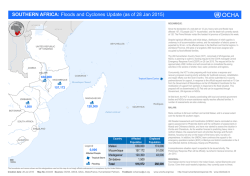


© Copyright 2026