1. Art and Diseño

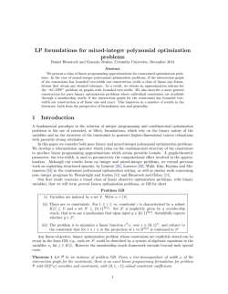
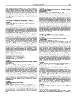
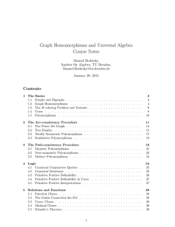
Efficient Search Space Exploration for HW-SW Partitioning
†
Sudarshan Banerjee
Nikil Dutt
Center for Embedded Computer Systems
University of California, Irvine, CA, USA
[email protected] [email protected]
ABSTRACT
graph DAG (directed acyclic graph) extracted from a sequential application written in ’C’ or any other procedural language, where the
graph vertices represent functions, and the graph edges represent
function calls or accesses between functions.
In this paper, we make two contributions to HW-SW partitioning.
First we prove that for a callgraph representation, when a vertex is
moved to a different partition, it is only necessary to update the
execution time change metric [6] for its immediate parents and immediate children instead of all ancestors along the path to the root.
This in general allows for a more efficient application of movebased algorithms like simulated annealing (SA).
Second, we present a cost function for simulated annealing to
search regions of the solution space often not thoroughly explored
by traditional cost functions. This enables us to frequently generate
more efficient design points.
Our two contributions result in a very fast simulated annealing
(SA) implementation that generates partitionings such that the application execution times are often better by over 10% compared to
a KLFM (Kernighan-Lin/Fiduccia-Matheyes) algorithm for HWSW partitioning for graphs ranging from 20 vertices to 1000 vertices. Equally importantly, graphs with a thousand vertices are processed in much less than a second.
Hardware/software (HW-SW) partitioning is a key problem in the
codesign of embedded systems, studied extensively in the past. One
major open challenge for traditional partitioning approaches – as
we move to more complex and heterogeneous SOCs – is the lack
of efficient exploration of the large space of possible HW/SW configurations, coupled with the inability to efficiently scale up with
larger problem sizes. In this paper, we make two contributions for
HW-SW partitioning of applications represented as procedural callgraphs: 1) we prove that during partitioning, the execution time
metric for moving a vertex needs to be updated only for the immediate neighbours of the vertex, rather than for all ancestors along
paths to the root vertex; consequently, we observe faster run-times
for move-based partitioning algorithms such as Simulated Annealing (SA), allowing call graphs with thousands of vertices to be processed in less than a second, and 2) we devise a new cost function
for SA that allows frequent discovery of better partitioning solutions by searching spaces overlooked by traditional SA cost functions. We present experimental results on a very large design space,
where several thousand configurations are explored in minutes as
compared to several hours or days using a traditional SA formulation. Furthermore, our approach is frequently able to locate better
design points with over 10 % improvement in application execution time compared to the solutions generated by a Kernighan-Lin
partitioning algorithm starting with an all-SW partitioning.
Categories and Subject Descriptors: B.6.3 [C.0]
General Terms: Algorithms
Keywords: HW-SW partitioning, dynamic cost function
1.
2. RELATED WORK
HW-SW partitioning is an extensively studied ”hard” problem
with a plethora of approaches- dynamic programming [11], genetic
algorithms [3], greedy heuristics [10], to name a few. Most of the
initial work, [11], [12], focussed on the problem of meeting timing constraints with a secondary goal of minimizing the amount
of hardware. Subsequently there has been a significant amount
of work on optimizing performance under area constraints, [1],
[2], [6]. With the goal of searching a larger design space, techniques such as simulated annealing (SA) have been applied to HWSW partitioning using fairly simple cost functions. While a lot
of initial work such as [12] was based exclusively on SA, recent
approaches commonly measure their quality against a SA implementation. For example, [1] compares simulated annealing with a
knowledge-based approach, and [2] compares SA with tabu search.
It is well-known that SA requires careful attention in formulating
a cost function that allows the search to ”hill-climb” over suboptimal solutions. However, much of the published work in HW-SW
partitioning have not studied in detail the SA cost functions that
permit a wider exploration of the search space. As an example, in
[2], [7], the SA formulation considers only valid solutions satisfying constraints, thus restricting the ability of SA to ”hill-climb”
over invalid solutions to reach a valid better solution.
The two previous pieces of work in HW-SW partitioning that are
most directly related to our work are [6], [4]. Our model for HWSW partitioning is based on [6], a well-known adaptation of the
INTRODUCTION
Partitioning is an important problem in all aspects of design.
HW-SW (hardware-software) partitioning, i.e, the decision to partition an application onto hardware (HW) and software (SW) execution units, is possibly the most critical decision in HW-SW codesign. The effectiveness of a HW-SW design in terms of system execution time, area, power consumption, etc, are primarily influenced
by partitioning decisions. In this paper, we consider the problem
of minimizing execution time of an application for a system with
hard area constraints. We consider an application specified as a call
†This work was partially supported by NSF Grants CCR-0203813
and ACI-0205712
Permission to make digital or hard copies of all or part of this work for
personal or classroom use is granted without fee provided that copies are
not made or distributed for profit or commercial advantage and that copies
bear this notice and the full citation on the first page. To copy otherwise, to
republish, to post on servers or to redistribute to lists, requires prior specific
permission and/or a fee.
CODES+ISSS’04, September 8–10, 2004, Stockholm, Sweden.
Copyright 2004 ACM 1-58113-937-3/04/0009 ...$5.00.
122
memory
v0
v4
v6
SW
access to the callee function v j from the caller function vi . The
SW execution times and callcounts are obtained from profiling the
application on the SW processor. In this model, the HW execution
time and the HW area for the functions are estimated from synthesis
of the functions on the given HW unit. The simple model for HW
area estimates assumes that the area of a cluster of components can
be obtained by summing the individual HW areas. Communication time estimates are made by simply dividing the volume of data
transferred by the bus speed. Since the execution time model is
sequential, bus contention is assumed to play an insignificant role.
Each edge ei j has 2 weights (cci j , cti j ). cci j represents the call
count, i.e, the number of times function v j is accessed by its parent
vi . cti j represents the HW-SW communication time, i.e, if vi is
mapped to SW and its child v j is mapped to HW (or vice-versa), cti j
represents the time taken to transfer data between the SW and the
HW unit for each call. (Note: we assume that vertices mapped onto
the same computing unit have negligible communication latency)
Each vertex vi has 3 weights (tis , tih , hi ). tis is the execution time
of the function corresponding to vi on the SW unit (processor). tih
and hi are the execution time, and, area requirement, respectively
for the function on the HW unit. Note that in this work we do
not consider compiler (synthesis) optimizations leading to multiple
HW implementations with different area and timing characteristics.
A partitioning of the vertices can be represented as P = {vs0 , vh1 , vs2 .....}.
This denotes that in partitioning P, vertex v0 is mapped to SW, v1
is mapped to HW, v2 is mapped to SW, etc. Two key attributes of
a partitioning are (T P , H P ). T P denotes the execution time of the
application under the partitioning P, H P denotes the aggregate area
of all components mapped to hardware under partitioning P.
HW local memory
HW
v3
v1
v2
Figure 1: Target architecture
SW
v5
HW
Figure 2: Simple callgraph
KL paradigm for HW-SW partitioning; our efforts in improving
the quality of the cost function are closely related to [4].
Our partitioning granularity is similar to [6], effectively that of
a loop-procedure call-graph; each partitioning object represents a
function and the DAG edges are annotated with callcounts. [6]
introduced the notion of execution time change metric for a DAG,
and updating the metric potentially by evaluation of ancestors along
the path to the root. The linear cost function in [6] ignores the effect
of HW area as long as the area constraint is satisfied.
[4] provides an in-depth discussion of cost functions and the notion of improving the results obtained from a simple linear cost
function by dynamically changing the weights of the variables. We
differ from [4] in the following ways: [4] addresses the problem of
choosing a suitable granularity for HW-SW partitioning that minimizes area while meeting timing constraints; since we consider
the problem of minimizing execution time while satisfying HW
area constraints, the proposed cost function in [4] needs significant
adaptation for our problem. In [4], the dynamic weighting technique was applied towards the secondary objective of minimizing
HW area once the primary objective, the timing constraint, was almost satisfied. We however, apply a dynamic weighting factor to
our cost functions in various regions of the search space to better
guide the search. Last but not the least, since their primary focus
was on the granularity selection problem, there was no quantitative
comparison of their approach with other algorithms- we have compared our approach to the KLFM approach with an extensive set of
test cases and demonstrated the effectiveness of our approach.
3.
4. EFFICIENT COMPUTATION OF EXECUTION TIME CHANGE METRIC
Given a sequential execution paradigm and a call-graph specification, the execution time of a vertex vi is computed as the sum of
its self-execution time and the execution time of its children. The
execution time for vi additionally includes HW-SW communication
time for each child of vi mapped to a different partition. Thus, if
TiP denotes the execution time for vertex vi under a partitioning P,
PROBLEM DESCRIPTION
We consider the problem of HW-SW partitioning of an application specified as a callgraph extracted from a sequential program
written in C, or, any other procedural language. For the purpose
of illustrating the basic partitioning formulation, we assume a simple target architecture that contains one SW processor and one HW
unit connected by a system bus, as shown in Figure 1. 1 We assume
mutually exclusive operation of the two units, i.e, the two units may
not be computing concurrently. We also assume that the HW unit
does not have dynamic RTR (run-time reconfiguration) capability.
The problem considered in this paper is to partition the application into HW and SW components such that the execution time
of the application is minimized while simultaneously satisfying the
hard area constraints of the HW unit. Essentially, given a software
program, we want to map as many functions as possible to the fixed
HW unit to improve program performance (thereby maximally utilizing available HW resources in a computing platform).
Preliminaries
The input to the partitioning algorithm is a directed acyclic graph
(DAG) representing a call-graph, CG = (V, E). V is the set of graph
vertices and E the set of edges. Each partitioning object corresponding to a vertex vi ∈ V is essentially a function that can be
mapped to HW or SW. Each edge ei j ∈ E represents a call or an
i
i
(cci j ∗ T j )+∑ j=1
(cci j ∗ cti j )
TiP = ti + ∑ j=1
h
s
where ti is either ti or ti depending on whether vi is currently
mapped to HW or SW in the partitioning P. Ci represents the set
di f f
represents the set of all children
of all children of vertex vi , Ci
of vi mapped to a different partition. Note that if v0 corresponds to
main in a ’C’ program, T0P equals the complete program execution
time when partitioning P specifies whether vertices are mapped to
HW or SW.
For a partitioning P, the execution time change metric ∆Pi , for a
vertex vi , is defined as the change in execution time when the vertex
vi is moved to a different partition. That is, ∆Pi denotes the change
in T0P when vertex vi is mapped to a different partition.
From the definition of the execution time change metric, it would
appear that when a vertex is moved to a different partition, the metric values for all its ancestors would need to be updated. Indeed, in
previous work, [6], the change equations assumed it was necessary
to update ancestors all the way to the root. In the simple example
shown in Figure 2, the execution time of the program (same as the
execution time for vertex v0 ) obviously depends on the execution
time of its descendant v2 . Let us assume all vertices were initially
in SW. If we move the vertex v2 to HW, the execution time changes
due to HW-SW communication on the edges (v3 , v2 ), (v1 , v2 ) and
change in execution time for vertex v2 . It would appear that any
execution time related metric for the vertices v0 , v6 , v4 , would need
|C |
1 Of course, our formulation can be extended to more contemporary
SoC’s containing multiple HW and SW components where we have
a fixed area constraint and want to maximize performance
123
|C di f f |
5. SIMULATED ANNEALING
to be updated when this move is made. This, however, is not the
case, as proved in the following lemma:
Lemma: For any two vertices vx and vy , if a vertex vx is
moved to a different partition, ∆y needs to be updated only if
there is an edge (x, y) or, (y, x). This update requires changing
exactly one term in ∆y , i.e this update can be done in O(1) time
per edge.
P ROOF. We define the aggregate call count, CCi for a vertex vi
|Pi |
in the following recursive manner: CCi = ∑ j=1
(cc ji ∗ CC j ). Pi
represents the set of all parent vertices (all functions it is called
from) for the vertex vi . CC0 , i.e the aggregate call count for the
root vertex, is 1.
CCi represents the exact number of times the function corresponding to vertex vi is called along all possible paths from the
root. Now, if we recursively expand T0P , an unrolled representation
for T0P is:
−−−−−−−−−−−−−−−−−−−
Algorithm SA
while (NOT EQUILIBRIUM)
For i = 1 to It
// iterations at current temperature
P’ = random perturbation of the current configuration, P
COST ∆ = COST(P’) - COST(P)
if (COST ∆ < 0) P = P’
else,
generate random number x ε [0,1]
∆
if (x < e−COST /T ) P = P’
endfor
UPDATE T () (from annealing schedule)
EVALUATE EQUILIBRIUM CONDITION()
endwhile
−−−−−−−−−−−−−−−−−−−
The above SA algorithm represents a typical formulation of simulated annealing for problems in combinatorial optimization, as initially proposed in [15]. The SA algorithm essentially tries to find an
optimal solution to a ”hard” problem such as partitioning, by conceptually representing the problem as a physical system with a huge
number of particles at an initial temperature T. The system is randomly perturbed and the temperature is successively decremented
allowing the system to reach statistical equilibrium at each temperature step: a state of minimal energy of the system corresponds to
an optimal solution to the ”hard” problem. Thus, key parameters in
any formulation are the initial temperature T, the cooling (annealing) schedule mandating how the temperature is decremented, and
the number of iterations at each temperature step.
In HW-SW partitioning, perturbation is commonly defined as a
move of a single vertex from HW to SW and vice versa, though experiments have been conducted with perturbations involving multiple moves [7]. A typical cost function is a linear combination of
normalized metrics [1], [4], [2]. For our problem, the two metrics
we need to consider are the execution time and the HW area.
For a SA approach to HW-SW partitioning, execution time is
primarily driven by the computation cost of the cost function. A
cost of O(E) to compute the execution time of a partitioning by a
traversal of the call-graph for every new configuration is too expensive for graphs with 100’s to 1000’s of vertices. For our problem,
we can simply use the execution time change metric defined earlier
to efficiently update the execution time for a new partitioning by
updating only the immediate neighbours of a vertex. Since the average indegree and outdegree of a call graph is expected to be a low
number, the average cost of a move is very low and enables the SA
algorithm to do a very rapid evaluation of the search space. Notationally, for a partitioning P with attributes (T P , H P ), a HW to SW
move of vertex vi generates a new partitioning P1 with attributes
(T P + ∆Pi , H P − hi ), and similarly for a SW to HW move.
5.1 Cost function for simulated annealing
Often, a statically weighted linear combination of metrics is used
as a cost function for SA algorithms in an attempt to overcome
its well-known limitations in handling multiobjective problems. In
this section we first provide the intuition for developing cost functions that explore points often not considered in traditional cost
functions, and then describe the cost function.
SA uses randomization to overcome local minima by accepting
suboptimal moves with some probability: our goal is to guide the
algorithm towards potentially more interesting design points by explicitly forcing the algorithm to accept apparently bad moves when
far away from the objective. Simultaneously, we force the algorithm to probabilistically reject some apparently good moves that
would always be accepted by most heuristics. As an example, when
T0P = ∑i=0 (CCi ∗ ti )+∑(i, j) ε E (δPij ∗CCi ∗ cti j ).
δPij is the Kronecker delta function defined for edge (i, j) in the
partitioning P - it takes a value of 1 if the vertex vi and its child
vertex v j are mapped to different partitions, 0 otherwise. The first
expression has exactly one term per vertex and the second expression has exactly one term per edge. If we now evaluate T0Px , the
new execution time when vertex vx is moved to generate the new
partitioning Px ,
(V −v )
T0Px =∑i=0 x (CCi ∗ ti ) + txPx ∗CCx +∑(i, j)ε(E−X )(δPij ∗CCi ∗
|V |
cti j )+∑(i, j) ε X (δPi jx ∗CCi ∗ cti j )
where X is the set of all edges adjacent to vertex vx , including its
immediate parents and immediate children. The Kronecker delta
values can change only for edges adjacent to vx . We can now evaluate ∆Px = T0Px − T0P corresponding to the change in execution time
when vertex vx is moved.
∆Px = CCx ∗ (txPx − tx )+∑(i, j) ε X ((δPi jx − δPij ) ∗CCi ∗ cti j )
We can similarly compute ∆Py for any other vertex vy as
∆Py = CCy ∗ (ty y − ty )+∑(i, j) ε Y ((δi jy − δPij ) ∗CCi ∗ cti j ) - Eqn (A)
P
P
P
Next, we evaluate the execution time T0 xy corresponding to the
new partitioning when vertex vx is moved, followed by vertex vy
being moved.
P
(V −v −v )
P
T0 xy = ∑i=0 x y (CCi ∗ ti ) + txPx ∗CCx + ty y ∗CCy +
∑(i, j)ε(E−X −Y)(δPij ∗ CCi ∗ cti j )+ ∑(i, j)ε(X −[x,y])(δPi j ∗ CCi ∗
x
cti j )+
∑(i, j)εY (δPi j
∗CCi ∗ cti j )
where [x, y] denotes either (x, y) or (y, x). Note that from our
problem definition we can not have both (x, y), and, (y, x).
P
Thus, we can compute ∆Py x = T0 xy − T0Px as
xy
P
∆Py x = CCy ∗ (ty y − ty ) −((i, j)=[x,y]) (δPi jx ∗CCi ∗ cti j )−
∑(i, j)ε(Y−[x,y]) (δPij ∗CCi ∗ cti j )+ ∑(i, j) ε Y (δPi j ∗CCi ∗ cti j )
P
P
= CCy ∗ (ty −ty )+∑(i, j)ε(Y−[x,y]) ((δi j − δPij ) ∗CCi ∗ cti j )+
xy
y
((i, j)=[x,y]) ((δPxy
ij
xy
− δPi jx ) ∗CCi ∗ cti j )
- Eqn (B)
δi j depends only on whether vertices vi and v j are in the same
P
partition, or in different partitions. That is, δi jxy = δPij if (i, j) =
[x, y]. So, comparing Equations (A) and (B), we have
P
P
∆Py x − ∆Py =((i, j)=[x,y]) ((δi jxy − δPi jx ) − (δi jy − δPij )) ∗CCi ∗ cti j
Thus we have proved that when vertex vx is moved to a different
partition, ∆y needs to be updated only if there is an edge [x, y]. Also,
the update involves changing exactly one term in ∆y .
Our experimental results will show that this result allows us to
have very fast run-times for move-based algorithms like SA.
124
execution time
better
Y
hardware area -->
,
worse
less time,
more area
P1
Ac
A.
Py
more time,
more area
x
+ B.
y
P4 HW
-+
++
P
--
Region A
less time,
less area
Tmin
P
Tmax
X
execution time -->
Figure 3: Solution space
P
+more time,
less area
P2
SW
P3
A.1
Figure 4: Neighbourhood move
x
- B.1
Pz
Px
y
Figure 5: Cost functions
Figure 5, that cause the execution time to deteriorate slightly but in
exchange free up a large amount of HW area. Such moves would
be probabilistically rejected by traditional cost functions that ignore
the HW area component, but we force their acceptance by explicitly introducing a cost function (A ∗ ∆T + B ∗ ∆A ), A >> B in the
quadrant (+t, −h).
(b) we reduce weightage on some moves like Py in Figure 5, that
improve execution time slightly but consume an additional large
amount of HW area. This is based on a similar reasoning of enabling the cost function to explore more combinatorial possibilities.
(c) we reduce weightage on some moves like Pz in Figure 5 that
improve the execution time slightly but free up a large amount of
HW area. We are now actually attempting to guide the search away
from making moves that do not appear to be headed towards our
desired solution space. Intuitively, for a partitioning where there
are relatively few HW components, the HW-SW communication
cost can potentially play a dominant role. For moves like Pz , freeing up a large amount of HW could potentially result in a slight
improvement in execution time due to significant reduction in HWSW communication. Blindly accepting such moves translates to
attempting to reduce communication cost between some vertex vx
mapped to HW and its neighbours in SW by moving back vx to SW.
When we are far from our desired solution space, we would instead
prefer to encourage the algorithm to reduce communication cost by
adding more of its neighbours to HW.
We next consider the notion of dynamically weighting the components of the cost function as suggested in [4]. This is a powerful
technique which essentially changes the slope of the line through
P, thus dynamically changing the search region. In [4], this technique was applied towards the secondary objective of minimizing
HW area once the primary objective, the timing constraint was almost satisfied. We however, apply a dynamic weighting factor to
our cost functions in various regions in an attempt to better guide
the search. Conceptually we dynamically weight the time component with the distance from the boundary in our attempt to guide
the search more towards the top left corner of the bounded region
A in Figure 3.
Among other key issues considered in our cost function are the
impact of boundary violations, i.e when a move leads us to a partitioning with HW area greater than the constraint. We penalize all
such moves with a factor proportional to the extent of the boundary
violation. We can clearly achieve this with a high weightage on
the area component , i.e., a function (A ∗ ∆T + B ∗ (Areanew − Ac )),
where B >>> A. Similarly when a move leads from an invalid
partitioning to a valid partitioning, we reward it with a factor proportional to the extent that it is inside the boundary.
Another important aspect of our cost function is the notion of
a threshold. When we are very close to the boundary, we need
a cost function that has only a slight bias towards the component
representing execution time. In our cost function, the time compo-
we are far away from our optimization goal, we would prefer not to
always accept a move that improves execution time only slightly at
the cost of a significant amount of hardware area.
Given our view of SA as a sequence of moves each of which is
blindly accepted, or probabilistically rejected depending upon its
degree of suboptimality, we define a cost function on the parameters that change for a given move, i.e, execution time, and HW
area. The change in execution time for a move, ∆T , is the same as
execution time change metric for the moved vertex. The change in
area, ∆A , is positive, hi for a SW-HW move, and negative, -hi for a
HW-SW move of vertex vi .
In Figure 3, each possible partitioning P is represented by a point
in the two-dimensional plane with x and y co-ordinates. The x-axis
represents the execution time corresponding to the given partitioning, while the y-axis represents the aggregate HW area. The vertical
lines Tmin and Tmax represent the execution times for an all HW and
an all SW solution respectively. The horizontal line Ac represents
the area constraint. To solve our problem of minimizing execution
time under a hard area constraint, we effectively need to search for
a point as close as possible to the upper left corner of the bounded
rectangular region A.
A move of a single component from SW to HW in partitioning P
is expected to lead to a new partitioning with improved (less) execution time and more HW area, such as P1 in Figure 4. Similarly, P2
corresponds to a HW to SW move with less HW area. More generally, when a single component in partitioning P is moved between
partitions, the new partitioning Pi lies in one of the four quadrants
centred at P. A partitioning P1 with improved execution time and
additional HW area lies in the quadrant (−t, +h), represented in
Figure 4 as (−, +). Similarly, a partitioning P2 with improved execution time and reduced HW area lies in the quadrant (−t, −h),
represented as (−, −), and so on for partitionings P3 , P4 .
We next consider the evaluation of a cost function (A ∗ ∆T + B ∗
∆A ) at the point P, corresponding to a random move generated by
the SA algorithm. A and B are weights that include the normalization factors required to be able to combine the two cost function
components which are in completely different units. This cost function is a simple straight line through P splitting the region around
P into 2 equal parts. In traditional cost functions like [6], where
the HW area component of the cost function is ignored as long as
the area constraint is satisfied, essentially every random move that
improves the execution time component of the cost function is accepted with a probability of 1. An example of such moves are P1 ,
P2 in Figure 4, i.e all moves lying in quadrants (−t, +h), (−t, −h),
represented in the figure as (−+), (−−).
If we now specifically consider a partitioning P in Figure 3 such
that few components have been mapped to HW, and the execution
time is hence expected to be closer to the SW execution time, our
goal is to bias the move acceptance such that:
(a) we provide additional weightage to some moves like Px in
125
Ac = 0.05
nent is dynamically weighted by the distance from the boundarywe have observed experimentally that close to the boundary, desirable weights for the time component in this region are even lower
than what our cost function provides. Thus, we needed to add the
notion of a threshold region very close to the boundary where we
explicitly assign a lower weightage to the time component of the
cost function.
Based on the above discussion, our cost function is algorithmically described as follows:
if (current partititioning is a valid solution)
if (move causes boundary violation)
Significant penalty proportional to area violation
(i)
else if (current partitioning is very near to boundary)
Slightly reduced weightage on time (as compared to (iii))
else
if (move in quadrant –)
(iii)
(A1 ∗ ∆T + B1 ∗ ∆A ), where A1 >> B1
else
(iv)
(A2 ∗ ∆T + B2 ∗ ∆A ),
else // (current partitioning lies outside boundary)
a mirror image of the above set of rules.
In Equations (iii) and (iv), the terms A1 and A2 are dynamically
weighted by the distance from the boundary. The HW area component of the cost function is normalized with respect to the areaConstraint. A more detailed description of the actual values implementing rules (i), (iii), etc, are in [18].
5.2 Key parameters in SA
In order to obtain quality results, we tuned the algorithm SA by
using the following parameter settings. For decrementing the temperature, we chose the popular geometric cooling schedule, where
the new temperature is given by Tnew = α ∗ T . α is a constant that
typically varies between 0.9 - 0.99. After a lot of experiments, we
fixed α at 0.96.
The stopping criterion is an important parameter, often formulated as the maximum number of moves that did not produce any
improvement in the solution. In previous work, this has typically
been a fixed number. We observed that this criterion has a strong
correlation with problem size and hence, we scale the criterion from
5000 moves without improvement for graphs with 50 vertices, to
15000 moves without improvement for graphs with a 1000 vertices.
Our experiments indicated that there was only a weak correlation
between the initial temperature and the problem size. So, we kept
the initial temperature T fixed at 5000.
Another key parameter that we have often found missing in previous work on HW-SW partitioning is the inner loop in Algorithm
SA where there are multiple iterations at each temperature. We have
observed experimentally that the solution quality degrades when
there is a single iteration at each temperature step as compared to
the approach of applying multiple iterations at each temperature
step.
6.
CCR=0.1
0.3
20
50
size=50
indeg=4
0.5
Ac = 0.3
0.7
100
200
500
outdeg=4
Ac = 0.6
1000
TGFF
0.5
20
0.7
50
indeg=4
Ac = 0.002
500
outdeg=10
CCR=0.1
1000
indeg=2
outdeg=5
indeg=5
outdeg=7
EXPERIMENTS
As shown in Figure 6, we explored a very large space of possible designs by generating graphs which varied the following set of
parameters: (1) varying indegree and outdegree (2) widely varying
number of vertices (3) varying CCRs (computation-to-communication
ratio). (4) varying area constraints.
We augmented the parameterizable graph generator TGFF [13]
to generate the graphs used in our experiments. An example of an
augmentation was one that enabled TGFF to generate HW execution times for vertices such that the HW execution time of a vertex
was faster than the SW execution time by a number between 3 and
8 times.
Let S = {20, 50, 100, 200, 500, 1000} denote the range of graph
126
0.5
Ac = 0.12
0.7
Ac = 0.25
Figure 6: Set of experiments
sizes generated where size corresponds approximately to the number of vertices in the graph. As an example, for a graph size 50,
TGFF generates a graph with between 48 to 52 vertices. We chose
S to observe how our algorithm worked on a large range of graph
sizes. Let CR = {0.1, 0.3, 0.5, 0.7} denote the set of CCR’s
(communication-to-computation ratio). The notion of CCR is very
important in partitioning and scheduling algorithms that consider
communication between tasks/functions. A CCR of 0.1 means
that on an average, communication between tasks/functions in a
call-graph/task graph requires 1/10’th the execution times of the
functions/tasks in the graph. As CCR increases, communication
starts playing a more important role in coarse-grain partitioning and
scheduling algorithms.
We generated data for over 12000 individual runs of the SA with
the following configurations from Figure 6.
Step 1 The maximum indegree and outdegree of a vertex were
set to 4 each, which are reasonably representative of realistic callgraphs. Corresponding to these fixed parameters, we generated a
set of graphs with the following characteristics. Each run of SA
chose a graph size from S = {20, 50, 100, 200, 500, 1000}; for each
graph size we chose CCR from CR = {0.1, 0.3, 0.5, 0.7} Thus, we
effectively generated a set of graphs |S| X |CR|. Note that in the
tables that follow, graphs with size 50 are denoted as v50, graphs
with size 100 are denoted as v100, etc.
Step 2 For each of the graphs generated in Step 1, we varied the
area constraint Ac as a percentage of the aggregate area needed to
map all the vertices to HW. On one extreme, we set Ac such that
very few partitioning objects would fit into HW, while at the other
extreme, a significant proportion of the objects would fit into HW.
Step 3 We repeated the above two steps with a maximum indegree
and outdegree of (i) 4 and 10 (ii) 2 and 5 (iii) 5 and 7.
Thus, the experimental data presented represents information collected from over 12000 experiments.
To measure the quality of results, we simply record the program
execution times computed by the SA algorithm with our new cost
function, and the KLFM algorithm as in [6]. In prior work, however, experiments to measure the quality of a partitioning algorithm
have often been formulated by forcing constraint violations and attempting to integrate the degree of violations into some unitless
number, as in [6], [1].
For a given design configuration, if Tkl is the execution time of
the partitioned application computed by the KLFM algorithm, and
Tsa is the execution time of the partitioned application computed
by the SA algorithm, our quality measure is the performance difference given by:
(Tkl − Tsa )/Tkl ∗ 100
Thus, a positive number, say, 5%, implies that the KLFM algorithm
computed an execution time better than SA by 5%, while a nega-
-5
SA better
-10
-15
BESTDEV
-20
0
0.1
0.2
0.3
0.4
0.5
Area Constraint- %
0.6
KLFM better
0
-5
SA better
-10
-15
-20
-25
0
-5
-10
0.1
0.2
0.3
0.4
0.5
SA better
-15
-20
-25
0
5
KLFM better
5
0.6
0
0.1
0.2
0.3
0.4
0.5
0.6
Area Constraint (% of aggregate area)
Area Constraint- %
Performance difference KLFM/SA
0
Performance difference KLFM/SA
Performance difference KLFM/SA
KLFM better
5
5
Performance difference KLFM/SA
10
WORSTDEV
10
KLFM better
0
SA better
-5
-10
-15
-20
-25
0
0.1
0.2
0.3
0.4
0.5
0.6
Area Constraint (% of aggregate area)
Figure 7:
v50, CCR
Figure 8:
v50, CCR Figure 9:
v50, CCR
Figure 10: v50, CCR
0.1:
Performance Vs
0.3:
Performance Vs 0.5:
Performance Vs
0.7: Performance Vs conconstraint
constraint
constraint
straint
Graph BESTDEV WORSTDEV
AVG
SA KFM
in a SA implementation that generates partitionings such that the
type
(%)
(%)
(%)
rt
rt
execution times are often better by 10 % over a KLFM algorithm
v20
-24.9%
12.3%
-4.17% .07
.05
for graphs ranging from 20 vertices to 1000 vertices. Equally imv50
-22.9%
6.7%
-5.75% .08
.05
portantly, the algorithm execution times are very fast- graphs with
v100
-18.2%
5.7%
-5.47% .1
.07
1000 vertices are processed in less than half a second. We believe
v200
-13.9%
4.3%
-3.74% .19
.11
that such a fast SA formulation makes it feasible to fine-tune the
v500
-16%
6.8%
-4.53% .25
.48
function further in a real design environment to generate partitionv1000
-13.7%
6.4%
-4.17% .36
1.6
ing solutions with a quality significantly better than that obtained
Table 1: Aggregate data for all graphs
from traditional KLFM implementations.
One important limitation of this work is a simple additive HW
tive number, say -10%, implies that the SA algorithm computed an
area estimation model that does not consider resource sharing- this
execution time better than the KLFM algorithm by 10%.
could potentially be overcome in a future implementation with an
While the results of all the experiments are too voluminous to
approach like [8].
present here (and are detailed in [18]), we present sample results
In the future, we plan to extend these concepts to systems where
for problem sizes v50 and also aggregate average over all experiHW and SW execute concurrently, i.e, consider scheduling issues
ments. Figure 7 represents the data collected for graphs with 50
as part of the problem formulation. Also, based on our learning
vertices, and a fixed CCR of 0.1 for various area constraints. The
experience of individually tuning a lot of different parameters in
x-axis corresponds to the various area constraints and the y-axis
SA, we would like to extend the cost function concepts developed
corresponds to the performance difference. In this figure, a sighere to algorithms with fewer tunable parameters.
nificant majority of points show negative performance difference
8. REFERENCES
(below 0)- this indicates that our SA formulation mostly generates
[1] M L Vallejo, J C Lopez, ”On the hardware-software partitioning problem:
better results than the KLFM algorithm. The point BESTDEV repSystem Modeling and partitioning techniques”, ACM TODAES, V-8, 2003
resents the best performance improvement by our SA formulation
[2] T Wiangtong, P Cheung, W Luk, ”Comparing three heuristic search methods
over the KLFM algorithm, while point WORSTDEV represents the
for functional partitioning in hardware-software codesign”, Jrnl Design
Automation for Embedded Systems, V-6, 2002
best solutions computed by the KLFM algorithm. Similarly, Fig[3] K Ben Chehida, M Auguin, ”HW/SW partitioning approach for reconfigurable
ure 8, Figure 9, Figure 10 represent the data for graphs with 50
system design”, CASES 2002
vertices and a CCR of 0.3, 0.5, 0.7 respectively.
[4] J Henkel, R Ernst, ”An approach to automated hardware/software partitioning
Figs 7-10 represent the data for graphs with 50 vertices, which
using a flexible granularity that is driven by high-level estimation Techniques”,
IEEE Trans.on VLSI, V-9, 2001
is only a fraction of the aggregate data. In Table 1, we provide
[5] J Henkel, R Ernst, ”A hardware/software partitioner using a dynamically
a summary of the aggregate data. The column header BEST DEV
determined granularity”, DAC 1997
represents the best improvement in execution time computed by
[6] F Vahid, T D Le, ”Extending the Kernighan-Lin heuristic for Hardware and
the SA algorithm compared to the KLFM algorithm for the set of
Software functional partitioning”, Jrnl Design Automation for Embedded
Systems, V-2, 1997
experiments represented by a row like v50. The column header
[7] P Eles, Z Peng, K Kuchinski, Doboli, ”System Level Hardware/Software
WORST DEV represents the best results produced by the KLFM
Partitioning based on simulated annealing and Tabu Search”, Jrnl Design
algorithm. The column header AV GDEV represents the average
Automation for Embedded Systems, V-2, 1997
deviation between the two algorithms. The column header rt repre[8] F Vahid, D Gajski, ”Incremental hardware estimation during
hardware/software functional partitioning”, IEEE Trans. VLSI, V-3, 1995
sents the average run-time of each algorithm in seconds, measured
[9] F Vahid, J Gong, D Gajski, ”A binary-constraint search algorithm for
on a SunOS 5.8 machine with a 502 Mhz Sparcv9 processor.
minimizing hardware during hardware-software partitioning”, EDAC 1994
Table 1 thus clearly shows that our SA formulation often com[10] A Kalavade, E Lee, ”A global criticality/Local Phase Driven algorithm for the
putes a better partitioning with over 10% improvement in execution
Constrained Hardware/Software partitioning problem”, CODES 1994
[11] R Ernst, J Henkel, T Benner, ”Hardware-software cosynthesis for
time compared to a KLFM formulation and moreover, processes
microcontrollers”, IEEE Design and Test,V-10, Dec 1993
graphs with a thousand vertices in less than half a second, enabling
[12] R Gupta, De Micheli, ”System-level synthesis using re-programmable
rapid exploration of a very large design space.
components”, EDAC 92
7.
CONCLUSION
[13] R P Dick, D L Rhodes, W Wolf, ”TGFF: task graphs for free”, CODES 1998
[14] D G Luenberger, ”Linear and non-Linear programming”, Addison-Wesley.
[15] S Kirkpatrick, C D Gelatt, M P Vechi, ”Optimization by simulated annealing”,
Science, V-220, 1983
[16] C M Fiduccia, R M Mattheyes, ”A Linear-time heuristic for improving
network partitions”, DAC, 1982
[17] B Kernighan, S Lin, ”An efficient heuristic procedure for partitioning graphs”,
The Bell System Technical Journal, V-29, 1970
[18] S Banerjee, N Dutt, ”Very fast simulated annealing for HW-SW partitioning”,
Technical Report CECS-TR-04-17. UC, Irvine.
In this paper, we made two contributions. We first proved that for
HW-SW partitioning of an application represented as a callgraph,
when a vertex is moved between partitions, it is necessary to update the execution time metric only for the immediate neighbours
of the vertex. We additionally developed a new cost function for
SA that attempts to explore regions of the search space often not
considered in other cost functions. Our two contributions result
127