1. Art and Diseño

CS246: Mining Massive Data Sets
Winter 2015
Problem Set 2
Due 5:00pm February 5, 2015
Only one late period is allowed for this homework (2/10).
General Instructions
These questions require thought, but do not require long answers. Please be as concise as
possible. Please fill the cover sheet and submit it as a front page with your answers. We
will subtract 2 points for failing to include the cover sheet. Include the names of your
collaborators (see the course website for the collaboration or honor code policy).
All students (Regular and SCPD) should submit their answers using Scoryst (see course
website FAQ for further instructions). This submission should include the source code you
used for the programming questions.
Additionally, all students (Regular and SCPD) should upload all code through a single text
file per question using the url below. Please do not use .pdf, .zip or .doc files for your code
upload.
Cover Sheet: http://cs246.stanford.edu/cover.pdf
Code (Snap) Upload: http://snap.stanford.edu/submit/
Assignment (Scoryst) Upload: https://scoryst.com/course/39/submit/
Questions
1
Recommendation Systems (25 points) [Clifford, Negar]
Consider a user-item bipartite graph where each edge in the graph between user U to item I,
indicates that user U likes item I. We also represent the ratings matrix for this set of users
and items as R, where each row in R corresponds to a user and each column corresponds to
an item. If user i likes item j, then Ri,j = 1, otherwise Ri,j = 0. Also assume we have m
users and n items, so matrix R is m × n.
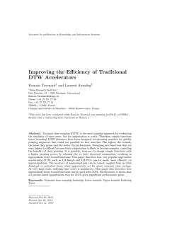
Let’s define matrix P , m × m as a diagonal matrix whose i-th diagonal element is the degree
of user node i, i.e. the number of items that user i likes. Similarly matrix Q, n × n is a
diagonal matrix whose i-th diagonal element is the degree of item node i or the number of
users that liked item i. See figure below for an example.
CS 246: Mining Massive Data Sets - Problem Set 2
2
Figure 1: User-Item bipartite graph.
(a) [5 points]
Let’s define the item similarity matrix, SI , n × n, such that the element in row i and column
j is the cosine similarity of item i and item j. Recall that the cosine similarity of two vectors
u·v 1
u and v is defined as kukkvk
Express SI in terms of R, P and Q. Your answer should be a
product of matrices, in particular you should not define each coefficient of SI individually.
Repeat the same question for user similarity matrix, SU where the element in row i and
column j is the cosine similarity of user i and user j.
Your answer should show how you derived the expressions.
(Note: To make the element-wise square root of a matrix, you may write it as matrix to the
power of 21 .)
(b) [5 points]
The recommendation method using user-user collaborative filtering for user u, can be described as follows: for all items s, compute ru,s = Σx∈users cos(x, u) ∗ Rxs and recommend the
top k items for which ru,s are the largest.
Similarly, the recommendation method using item-item collaborative filtering for user u can
1
The definition of cosine simiarity we saw in class took the arc-cos of this expression. The definition we
use here gives the same relative ordering, since the dot products are always positive in this case.
CS 246: Mining Massive Data Sets - Problem Set 2
3
be described as follows: for all items s, compute ru,s = Σx∈items Rux ∗cos(x, s) and recommend
the the top k items for which ru,s are the largest.
Let’s define the recommendation matrix, Γ, m × n, such that Γ(i, j) = ri,j . Find Γ for both
item-item and user-user collaborative filtering approaches, in terms of R, P and Q.
Your answer should show how you derived the expressions.
(c) [5 points]
Define the non-normalized user similarity matrix T = R ∗ RT . Explain the meaning of Tii
and Tij (i 6= j), in terms of bipartite graph structures (See Figure 1) (e.g. node degrees,
path between nodes, etc.).
(d) [10 points]
In this question you will apply these methods to a real dataset. The data contains information
about TV shows. More precisely, for 9985 users and 563 popular TV shows, we know if a
given user watched a given show over a 3 month period.
Download the dataset2 on http://snap.stanford.edu/class/cs246-data/hw2-q1-dataset.
zip.
The ZIP file contains:
• user-shows.txt This is the ratings matrix R, where each row corresponds to a user
and each column corresponds to a TV show. Rij = 1 if user i watched the show j over
a period of three months. The columns are separated by a space.
• shows.txt This is a file containing the titles of the TV shows, in the same order as
the columns of R.
We will compare the user-user and item-item collaborative filtering recommendations for the
500th user of the dataset. Let’s call him Alex.
In order to do so, we have erased the first 100 entries of Alex’s row in the matrix, and replaced
them by 0s. This means that we don’t know which of the first 100 shows Alex has watched
or not. Based on Alex’s behaviour on the other shows, we will give Alex recommendations
on the first 100 shows. We will then see if our recommendations match what Alex had in
fact watched.
• Compute the matrices P and Q.
2
The original data is from Chris Volinksy’s website at http://www2.research.att.com/~volinsky/
DataMining/Columbia2011/HW/HW6.html.
CS 246: Mining Massive Data Sets - Problem Set 2
4
• Using the formulas found in part (b), compute Γ for the user-user collaborative filtering.
Let S denote the set of the first 100 shows (the first 100 columns of the matrix). From
all the TV shows in S, which are the five that have the highest similarity scores for
Alex? What are their similarity score? In case of ties between two shows, choose the
one with smaller index. Do not write the index of the TV shows, write their names
using the file shows.txt.
• Compute the matrix Γ for the movie-movie collaborative filtering. From all the TV
shows in S, which are the five that have the highest similarity scores for Alex? In
case of ties between two shows, choose the one with smaller index. Again, hand in the
names of the shows and their similarity score.
Alex’s original row is given in the file alex.txt. For a given number k, the true positive
rate at top-k is defined as follows: using the matrix Γ computed previously, compute the
top-k TV shows in S that are most similar to Alex (break ties as before). The true positive
rate is the number of top-k TV shows that were watched by Alex in reality, divided by the
total number of shows he watched in the held out 100 shows.
• Plot the true positive rate at top-k (defined above) as a function of k, for k ∈ [1, 19],
with predictions obtained by the user-user collaborative filtering.
• On the same figure, plot the true positive rate at top-k as a function of k, for k ∈ [1, 19],
with predictions obtained by the item-item collaborative filtering.
• Briefly comment on your results (one sentence is enough).
What to submit:
(a) Expression of SI and SU in terms of R, P and Q and accompanying explanation
(b) Expression of Γ in terms of R, P and Q and accompanying explanation
(c) Interpretation of Tii and Tij
(d) The answer to this question should include the followings:
• The five TV shows that have the highest similarity scores for Alex for the user-user
collaborative filtering.
• The five TV shows that have the highest similarity scores for Alex for the item-item
collaborative filtering.
• The graph of the true positive rate at top-k for both the user-user and the item-item
collaborative filtering.
• A brief comment on this graph.
• Submit the source code via the SNAP electronic submission website and attach to
your Scoryst submission as well.
CS 246: Mining Massive Data Sets - Problem Set 2
2
5
Singular Value Decomposition (25 points + 5 extra
credit points) [Hristo, Peter]
In this problem we will explore SVD and its relationships to eigenvalue decomposition and
linear regression and show that it gives an optimal low rank approximation to a matrix.
First, recall that the eigenvalue decomposition of a real, symmetric, and square matrix
B ∈ Rd×d decomposes it into the product
B = QΣQT
where Σ = diag(λ1 , . . . , λd ) contains the eigenvalues of B (which are always real) along its
main diagonal and Q is an orthogonal matrix containing the eigenvectors of B as its columns.
When B has rank r < d we will often be concerned only with the non-zero eigenvalues (and
corresponding eigenvectors). In this case we take the term “non-zero eigenvectors” to mean
eigenvectors corresponding to non-zero eigenvalues.
We will start by showing how to compute the SVD of a matrix A ∈ Rm×n via eigenvalue
decomposition. This technique is particularly useful when one dimension of A is much larger
than the other (i.e. m n or vice versa). For concreteness, we will assume that m = 100
and n = 10, 000 (A is a wide matrix) and that it has rank r ≤ m. Let A = U SV T be the
SVD of A so that U ∈ Rm×r , S = diag(σ1 , . . . , σr ) contains the singular values of A, and
V ∈ Rn×r . Note that both, U and V , have orthonormal columns so that U T U = V T V = Ir
but that the rows of these matrices are not necessarily orthonormal.
(a) [12 points]
Finding the SVD using AAT or AT A:
1. Show that the matrices C = AT A and K = AAT are symmetric, and express the
non-zero eigenvalues and eigenvectors of these matrices in terms of U, S, V from the
SVD of A.
2. Suppose that we are only interested in the singular values of A. It takes O(d3 ) operations to find the eigenvalues of a symmetric d × d matrix. Should we use C or K to
find the singular values of A?
3. Show how to extract U and V using only the matrix A and the eigenvalue decomposition of C.
4. Show how to extract U and V using only the matrix A and the eigenvalue decomposition of K.
CS 246: Mining Massive Data Sets - Problem Set 2
6
(b)[13 points]
Document similarity using SVD:
In this exercise, you will play around with the SVD on some real data. To complete the
problem it will be the easiest to use Matlab. In Matlab the SVD of a matrix A can be
retrieved as: [U, S, V] = svd(A, ‘econ’); If you do not have access to Matlab you can
also use the open source “Matlab” implementation called Octave. You can also use any other
software package/language.
First, download the input file http://snap.stanford.edu/class/cs246-data/hw2_q2-Data.
zip 3 which is a normalized document-term incidence matrix X of various IMDb movie reviews. Here, each of the rows i can be considered to be a document di while the columns
represent the occurrence of words within the corresponding document. Alongside X is a
vector of binary labels y where yi = 1 indicates that review i liked its movie and yi = −1
indicates that review i disliked the movie.
Let X = U SV T be the SVD of X and define U (k) to be the k columns of U corresponding
to the k largest singular values of X. The matrix U (k) gives a k-dimensional representation
of the reviews where U (k)i , i.e. row i of U (k), is a k-dimensional vector that corresponds to
the ith review. We want to figure out how well this decomposition performs when identifying
positive and
negative reviews as our feature representation increases in dimensionality. Define
P640
w(k) = P
i=41 yi U (k)i to be a simple classifier built on reviews 41 through 640 and let
T
r(k) = − 40
i=1 yi U (k)i w(k) be a measure of the agreement between the predicted and
actual sentiment of the first 40 reviews, where lower is better. Compute r(k) for k =
{1, 21, 41, . . . , 601} and plot a graph showing how r changes as k varies.
(c) Extra Credit [5 points]
This is a hard (but nice) problem. Only attempt it if you have extra time after you finished
all other problems.
SVD for rank reduction:
We will show that the SVD gives an optimal low rank approximation of a matrix A ∈ Rm×n .
Along the way we will also explore its relationship to linear regression. In particular, we are
interested in finding matrices X ∈ Rm×k , W ∈ Rk×n , where k ≤ rank(A) is given, that solve
minimizekA − XW k2F .
X T X=Ik
(1)
P
Here k · k2F extends the vector L2 -norm to matrices in that kAk2F = ni=1 kai k22 where the ai
are the columns of A. Note that we require X to be orthogonal for convention4 .
3
Original dataset received from Hristo Paskov
ˆ W
ˆ ) that minimizes (1) in which X is not orthogonal, we can always come up with
Given a solution (X,
ˆ = P ΣRT is the SVD of X,
ˆ we set X = P and W = ΣRT W
ˆ so that X is
an orthogonal solution. If X
4
CS 246: Mining Massive Data Sets - Problem Set 2
7
Assuming that the SVD A = U SV T stores the singular values (and corresponding singular
vectors) in decreasing order5 , we will show that if U˜ , V˜ are the first k columns of U, V ,
respectively, and S˜ = diag(σ1 , . . . , σk ), then (X = U˜ , W = S˜V˜ T ) are optimal for (1).
1. Given a vector y ∈ Rm and a matrix Z ∈ Rm×d of features, linear regression finds
a coefficient vector w ∈ Rd that approximates y linearly based on Z. The vector w
minimizes ky − Zwk22 and, assuming rank(Z) = d, w can be expressed as
w = (Z T Z)−1 Z T y.
Assuming X is fixed in equation (1), give a closed form expression for W in terms of
A and X.
2. Suppose that we set X = U˜ , which was defined as the first k columns of the SVD of
X. Use your formula from above to give a simple expression for W in terms of S˜ and
V˜ .
3. We now turn to solving for X and no longer assume it is fixed. Use your solution to
part 1 above to eliminate W from (1) and express it in the form minX T X=Ik kM Ak2F
where M is a simple expression involving only product(s) and sum(s) of X. (Answers
involving inverses will not get full credit.)
4. An alternative way to characterize the k largest eigenvectors6 of a symmetric matrix
M ∈ Rm×m is via the problem maxQT Q=Ik trace(QT M Q) where Q ∈ Rm×k . Using your
expression from the previous question, show that problem (1) can be expressed as the
eigenvalue problem maxX T X=Ik trace(X T AAT X). You will need to use the fact that
kM k2F = trace(M T M ) and the properties of the trace7 .
5. Finally, use what you have proved here and in part (a) to conclude that X = U˜ and
W = S˜V˜ T .
What to submit:
1. Part(a): Written solution to questions (1) to (4).
2. Part(b): The plot of r as a function of k and submit the source code via the electronic
submission website.
3. Part(c): Written solution to questions (1) to (5).
ˆW
ˆ.
orthogonal and XW = X
5
i.e. S = diag(σ1 , . . . , σr ) with σ1 ≥ σ2 ≥ · · · ≥ σr .
6
i.e. eigenvectors corresponding to the k largest eigenvalues.
7
i.e. trace(M ) = trace(M T ) for square M , trace(BCD) = trace(DBC) = trace(CDB), and trace(A +
B) = trace(A) + trace(B).
CS 246: Mining Massive Data Sets - Problem Set 2
3
8
Theory of k-means (20 points) [Clement, Jean-Yves]
In this problem, we study two different initialization methods for the k-means algorithm.
First, let us set up the problem: we have a set X of n data points in the d-dimensional space
Rd . We are also given k, the number of clusters, and would like to choose a set of k centers
C to minimize the cost function:
X
φ=
min ||x − c||2
x∈X
c∈C
Then, the k-means algorithm for the above problem works as follows:
1. Initialization: Arbitrarily choose k initial centers C = {c1 , c2 , . . . , ck }
2. ∀ i ∈ {1, 2, . . . , k}, set the cluster Ci = x ∈ X |argmin1≤j≤k {||x − cj ||} = i
P
3. ∀ i ∈ {1, 2, . . . , k}, set ci to be the center of mass of Ci , that is ci = |C1i | x∈Ci x
4. Repeat steps 2 and 3 until C no longer changes.
We first prove some basic facts about this algorithm.
(a)[5 points]
Assume S is an arbitrary set of points (in Rd ) with center of mass c(S), and assume z is an
arbitrary point (not necessarily in S). The notation || · || denoting the L2 norm, first prove
that:
X
X
||x − z||2 −
||x − c(S)||2 = |S| · ||c(S) − z||2 .
x∈S
x∈S
(b)[5 points]
We denote by a superscript (t) the state of the k-means algorithm at the beginning of
iteration t. Prove that, while C (t) keeps changing, each iteration of
Pthe k-means algorithm
(t)
decreases the cost, i.e. prove that for each iteration t (where φ = x∈X minc∈C (t) ||x − c||2 ),
we have φ(t) ≥ φ(t+1) .
(c)[5 points]
Prove that when running k-means, the cost function φ converges to a finite value. (This
claims holds independently from the dataset and the initial clusters.)
Finally, argue8 that k-means converges, i.e. that the algorithm reaches a state where the
centroids (or equivalently the assignments of points to clusters) do not change.
8
For this part of the question, we expect more of a heuristic than a completely formal proof.
CS 246: Mining Massive Data Sets - Problem Set 2
9
(d)[5 points]
With an example show that with a bad initialization, the k-means algorithm may converge
to a clustering that has an unboundedly larger cost than the optimal clustering (i.e., the one
with the optimal cost). In other words, given an arbitrary number r > 1, give a situation
where k-means converges to a clustering whose cost is at least r times larger than the cost
of the optimal clustering. You may fix k.
(Note: A hard-coded example or the output of a coding example that behaves badly would
not receive full credit. We are asking for a formal example that can work for any arbitrary
number r > 1, and a formal analysis of the performance of the k-means algorithm.)
What to submit:
(a) Proof that
P
x∈S
||x − z||2 −
P
x∈S
||x − c(S)||2 = |S| · ||c(S) − z||2
(b) Proof that the cost of k-means decreases at each iteration
(c) Proof that the cost function always converges and argument that the cluster assignments
also converge.
(d) Formal example that leads to non-optimal convergence and analysis
4
k-means on MapReduce (30 points) [Janice, James,
Dima, Nat]
Automatic tagging and cross-linking of documents: Clustering algorithms are frequently used to automatically categorize documents by web services which receive a large
number of new content items daily. As human intervention would be very expensive, these
services need an automated way to find related items and to categorize and cross-link the
documents. News-aggregation site feedly is an example service which processes and categorizes tens of thousands of new documents per day.
We will explore this use case in this problem.
(a) [10 pts]
k-Means clustering on Hadoop: Implement the k-means using Map Reduce where a
single step of Map Reduce completes one iteration of the k-means algorithm. So, to run
k-means for i iterations, you will have to run a sequence of i MapReduce jobs.
Run the k-Means algorithm on Hadoop to find the centroids for the dataset at: http:
//snap.stanford.edu/class/cs246-data/hw2-q4-kmeans.zip
The zip has 4 files:
CS 246: Mining Massive Data Sets - Problem Set 2
10
1. data.txt contains the dataset which has 4601 rows and 58 columns. Each row is a
document represented as a 58 dimensional vector of features. Each component in the
vector represents the importance of a word in the document.
2. vocab.txt contains the words used for generating the document vector. (For example
the first word represents the first feature of the document vector. For document 2 (line
2 in data.txt), feature 3 “alkalemia” (line 3 in vocab.txt) has frequency 0.5, so the
third component of the document vector is 0.5.)
3. c1.txt contains k initial cluster centroids. These centroids were chosen by selecting
k = 10 random points from the input data.
4. c2.txt contains initial cluster centroids which are as far apart as possible. (You can
do this by choosing 1st centroid c1 randomly, and then finding the point c2 that is
farthest from c1, then selecting c3 which is farthest from c1 and c2, and so on).
Use Euclidean distance (ie, the L2 norm) as the distance measure. Set number of iterations
to 20 and number of clusters to 10. Use points in c1.txt for initialization.
Hint about job chaining:
We need to run a sequence of Hadoop jobs where the output of one job will be the input for
the next one. There are multiple ways to do this and you are free to use any method you
are comfortable with. One simple way to handle a such a multistage job is to configure the
output path of the first job to be the input path of the second and so on.
The following pseudo code demonstrates job chaining.
var inputDir
var outputDir
var centroidDir
for i in no-of-iterations (
Configure job here with all params
Set job input directory = inputDir
Set job output directory = outputDir + i
Run job
centroidDir = outputDir + i
)
You will also need to share the location of centroid file with the mapper. There are many
ways to do this and you can use any method you find suitable. One way is to use the Hadoop
Configuration object. You can set it as a property in the Configuration object and retrieve
the property value in the Mapper setup function.
For more details see :
CS 246: Mining Massive Data Sets - Problem Set 2
11
1. http://hadoop.apache.org/docs/r1.0.4/api/org/apache/hadoop/conf/Configuration.
html#set(java.lang.String,java.lang.String)
2. http://hadoop.apache.org/docs/r1.0.4/api/org/apache/hadoop/conf/Configuration.
html#get(java.lang.String)
3. http://hadoop.apache.org/docs/r1.0.4/api/org/apache/hadoop/mapreduce/Mapper.
html#setup(org.apache.hadoop.mapreduce.Mapper.Context)
Cluster Initialization strategies: The output of k-Means algorithm depends on the initial
points chosen. There are many ways of choosing the initial points. We will compare two of
them: random selection, and selecting points as far apart as possible.
(b) [5 pts]
For every iteration, compute the cost function φ(i) (as defined at the beginning of question
3). This means that, for your first MapReduce job iteration, you’ll be computing the cost
function using the initial centroids located in one of the two text files. Run the k-means on
data.txt using c1.txt and c2.txt. Generate a graph where you plot the cost function φ(i)
as a function of the number of iterations i=1..20 for c1.txt and also for c2.txt.
(Hint: Note that you do not need to write a separate MapReduce job to do this. You can
incorporate the computation of φ(i) into the Mapper/Reducer from part (a).)
(c) [5 pts]
Is random initialization of k-means using c1.txt better than initialization using c2.txt in
terms of cost φ(i)? Why? What is the percentage change in cost from using the initial
centroids versus using those centroids obtained after 10 iterations of K-Means?
Automatically tagging documents: One way of tagging documents is to assign word tags
to each cluster. To get the top k word tags for a cluster, sort the features for its centroid by
their coordinate values in descending order, choose the top k features and use words from
vocab.txt to get the word tags for these top k features.
For e.g. if the indexes of top 5 features of the centroid for cluster 1 are [1, 2, 6, 7, 10]
then the tags for the documents in cluster 1 are [activator, decay-corrected, softer,
mitomycin, spc] which are words at line 1, 2, 6, 7, 10 respectively in vocab.txt.
Use points in c1.txt for initialization.
(d) [10 pts]
Which 5 tags would you apply to the second document? For verification, the 10th tag is
alkalemia.
CS 246: Mining Massive Data Sets - Problem Set 2
12
What to submit:
(a) Code (both on your Scoryst submission and SNAP upload)
(b) Code (both on your Scoryst submission and SNAP upload), and graph for initialization
strategies
(c) The answer should include percentage improvement values and your explanation.
(d) 5 best tags