
1 Calculus TE - Teaching Tips
Calculus Teacher’s Edition Andrew Dreyfuss, (AndrewD) Jared Prolo, (JaredP) Ramesh Narasimhan, (RameshN) Say Thanks to the Authors Click http://www.ck12.org/saythanks (No sign in required) www.ck12.org To access a customizable version of this book, as well as other interactive content, visit www.ck12.org CK-12 Foundation is a non-profit organization with a mission to reduce the cost of textbook materials for the K-12 market both in the U.S. and worldwide. Using an open-content, web-based collaborative model termed the FlexBook®, CK-12 intends to pioneer the generation and distribution of high-quality educational content that will serve both as core text as well as provide an adaptive environment for learning, powered through the FlexBook Platform®. Copyright © 2012 CK-12 Foundation, www.ck12.org The names “CK-12” and “CK12” and associated logos and the terms “FlexBook®” and “FlexBook Platform®” (collectively “CK-12 Marks”) are trademarks and service marks of CK-12 Foundation and are protected by federal, state, and international laws. Any form of reproduction of this book in any format or medium, in whole or in sections must include the referral attribution link http://www.ck12.org/saythanks (placed in a visible location) in addition to the following terms. Except as otherwise noted, all CK-12 Content (including CK-12 Curriculum Material) is made available to Users in accordance with the Creative Commons Attribution/NonCommercial/Share Alike 3.0 Unported (CC BY-NC-SA) License (http://creativecommons.org/licenses/by-nc-sa/3.0/), as amended and updated by Creative Commons from time to time (the “CC License”), which is incorporated herein by this reference. Complete terms can be found at http://www.ck12.org/terms. Printed: May 15, 2012 iii AUTHORS Andrew Dreyfuss, (AndrewD) Jared Prolo, (JaredP) Ramesh Narasimhan, (RameshN) iv 1 2 3 4 5 www.ck12.org Calculus TE - Teaching Tips 1 1.1 2 Calculus TE Teaching Tips . . . . . . . . . . . . . . . . . . . . . . . . . . . . . . . . . . . . . . . Calculus TE - Common Errors 27 2.1 28 Functions, Limits, and Continuity . . . . . . . . . . . . . . . . . . . . . . . . . . . . . . . . . . . Calculus TE - Enrichment 29 3.1 Functions, Limits, and Continuity . . . . . . . . . . . . . . . . . . . . . . . . . . . . . . . . . . . 30 3.2 Differentiation . . . . . . . . . . . . . . . . . . . . . . . . . . . . . . . . . . . . . . . . . . . . . . 38 3.3 Applications of Derivatives . . . . . . . . . . . . . . . . . . . . . . . . . . . . . . . . . . . . . . . 45 3.4 Integration . . . . . . . . . . . . . . . . . . . . . . . . . . . . . . . . . . . . . . . . . . . . . . . . 51 3.5 Applications of Definite Integrals . . . . . . . . . . . . . . . . . . . . . . . . . . . . . . . . . . . . 58 3.6 Transcendental Functions . . . . . . . . . . . . . . . . . . . . . . . . . . . . . . . . . . . . . . . . 63 3.7 Integration Techniques . . . . . . . . . . . . . . . . . . . . . . . . . . . . . . . . . . . . . . . . . 67 3.8 Infinite Series . . . . . . . . . . . . . . . . . . . . . . . . . . . . . . . . . . . . . . . . . . . . . . 72 Calculus TE - Differentiated Instruction 78 4.1 Functions, Limits, and Continuity . . . . . . . . . . . . . . . . . . . . . . . . . . . . . . . . . . . 79 4.2 Derivatives . . . . . . . . . . . . . . . . . . . . . . . . . . . . . . . . . . . . . . . . . . . . . . . 93 4.3 Applications of Derivatives . . . . . . . . . . . . . . . . . . . . . . . . . . . . . . . . . . . . . . . 105 4.4 Integration . . . . . . . . . . . . . . . . . . . . . . . . . . . . . . . . . . . . . . . . . . . . . . . . 115 4.5 Applications of Definite Integrals . . . . . . . . . . . . . . . . . . . . . . . . . . . . . . . . . . . . 124 4.6 Transcendental Functions . . . . . . . . . . . . . . . . . . . . . . . . . . . . . . . . . . . . . . . . 134 4.7 Integration Techniques . . . . . . . . . . . . . . . . . . . . . . . . . . . . . . . . . . . . . . . . . 141 4.8 Infinite Series . . . . . . . . . . . . . . . . . . . . . . . . . . . . . . . . . . . . . . . . . . . . . . 151 Calculus TE - Problem Solving 162 5.1 Functions, Limits, and Continuity . . . . . . . . . . . . . . . . . . . . . . . . . . . . . . . . . . . 165 5.2 Differentiation . . . . . . . . . . . . . . . . . . . . . . . . . . . . . . . . . . . . . . . . . . . . . . 173 5.3 Applications of Derivatives . . . . . . . . . . . . . . . . . . . . . . . . . . . . . . . . . . . . . . . 180 5.4 Integration . . . . . . . . . . . . . . . . . . . . . . . . . . . . . . . . . . . . . . . . . . . . . . . . 190 www.ck12.org v 5.5 Applications of Integration . . . . . . . . . . . . . . . . . . . . . . . . . . . . . . . . . . . . . . . 195 5.6 Transcendental Functions . . . . . . . . . . . . . . . . . . . . . . . . . . . . . . . . . . . . . . . . 201 5.7 Integration Techniques . . . . . . . . . . . . . . . . . . . . . . . . . . . . . . . . . . . . . . . . . 204 5.8 Infinite Series . . . . . . . . . . . . . . . . . . . . . . . . . . . . . . . . . . . . . . . . . . . . . . 212 www.ck12.org C HAPTER 1 1 Calculus TE - Teaching Tips C HAPTER O UTLINE 1.1 C ALCULUS TE T EACHING T IPS CHAPTER 1. CALCULUS TE - TEACHING TIPS 2 www.ck12.org 1.1 Calculus TE Teaching Tips This Calculus Teaching Tips FlexBook is one of seven Teacher’s Edition FlexBooks that accompany the CK-12 Foundation’s Calculus Student Edition. To receive information regarding upcoming FlexBooks or to receive the available Assessment and Solution Key FlexBooks for this program please write to us at [email protected]. Lesson 1: Equations and Graphs It is almost cliché how math courses start out with a review of material from previous years. Students are out of practice and never seem to have either been taught, or don’t remember what has happened in previous classes (and will always claim to have not been taught it if they don’t remember). There are two considerations here as the calculus course starts. First, a complete calculus course is a full years worth of university material. This means that the course is conducted at a faster pace than high school students are used to. Compounding the problem for many classes is the even shorter year with the AP examination. Therefore, it is dangerous to get bogged down in the preliminaries. However, a strong case can be made that not much can be accomplished in a calculus class without a firm grounding in the fundamentals presented here. To have a conceptual understanding of functions and graphs is essential to gaining mastery of the basis for the limit, derivative and integral. In case of limited time, the key idea that needs to be driven home is how the relationship between the two variables creates a graph, and what the line means. The way that limits, derivatives and integrals are presented in a first course of calculus is all graphical. If students do not understand what they are looking at when the text later talks about zooming in on an area, strictly increasing or looking at activity at a minimum or maximum, to name a few examples, the key concepts will be lost. Graphing calculators can be valuable tools at this point, especially as they allow for fast manipulation of accurate graphs. There is some danger in relying too much on the graphing calculator, however. I have observed students who have done all of their graphing since linear function on graphing calculators and they end up with some peculiar habits. The most noticeable of which is losing track of the activity of a function outside of the domain graphed, lack of understanding of what happens near vertical asymptotes (the calculator often shows a continuous line), and an over reliance on guess and check methods, especially when the student gets to the chapter on extrema. Use the graphing tool to illustrate some key concepts quickly, check work done by hand, and use some of the calculation tools that may be useful on the university examination of choice, but make sure everything could theoretically be done by hand. Lesson 2: Relations and Functions While it may seem like an issue of semantics, I encourage my students to use, and try to use exact terminology when talking about mathematical relationships. The terms “expression”, “equation”, and “function” all have specific meaning. Students will often confuse them, or believe they can be used interchangeably. Knowing the difference pays off later in sections on inverse and transcendental functions. It is also useful when it comes to writing clear solutions, especially those with prose attached, because they author can then be absolutely clear, presenting work in an easy to follow manner. 1.1. CALCULUS TE TEACHING TIPS www.ck12.org 3 There is some inconsistency in the way students are taught to express intervals; the topic is pertinent here in expressing the domain and range of functions. The text uses mostly the inequality notation to state which numbers act as endpoints for each variable. Another option is to use the strict set notation with the parenthesis for not inclusive intervals and brackets for inclusive intervals, with the union set operator to join discreet intervals. Example: D = {−3 < x ≤ 0, 1 ≤ x < 2} = (−3, 0] ∪ [1, 2) There are also the standard sets that have defined bold-face letters: R = Real numbers, Q = Rational numbers, Z = Integers, N = Natural numbers. None of this is important to drive home to students except for the fact that a textbook, or instructor, often chooses one notation method and sticks to it. Different texts and classes may have different notations so students should be at least aware of the different choices. Speaking of notation, the different forms for writing the operation of composition for functions is a source of potential confusion for many students. The operator: ( f ◦ g)(x) tends to cause all kinds of problems. First, it looks like even more of a product than a single function. Second, we do everything left to right, but the action here is more right to left, made even worse by the fact that composition is one of the few non communicative operations that students have yet come across. Please use, and have students convert to, the nested notation, where the previously mentioned operation is equivalent to f (g(x)). This is clearer because the function g(x) is placed into the function f as if it were the variable, just like the composition is written. Lesson 3: Models and Data One of the tough things for students to do at this point is to have a sense for function behavior given a set of data points. The best tool is experience, of which the students are at a disadvantage. There are a few rules of thumb to help them out. • Population and monetary (interest, investment) data sets are almost always modeled with exponential functions. • Repeating data sets, like measurements taken every hour for a day, every month for a year etc., are almost always modeled by periodic functions. • Look at the difference in endpoints for suspected linear functions. The change in values on each extreme end will be the same for linear functions and no others. The text recommends plotting the point in either a calculator or by hand to choose a model based on the shape of the graph. This is often a useful task, but one with a chance to be misleading. The scaling of each axis can determine the shape of the graph sometimes more than the data points themselves. There is no clear rule for determining the correct scaling, other than choose endpoints far enough to show all the data points, so again experience and trial and error are the best tools. It is useful to use different scaling to see if it appears to change the shape of the graph. Linear functions will always appear to be linear, regardless of scaling (unless the data points vary substantially and you are zoomed in very “close”), where other functions may appear to be linear at some scales, but their curves will appear at others. Also, filling the screen as best you can will often help. Something to remember is that the functions are not meant to be perfect reflections of observed phenomena, but useable models for a defined range. Negative time may not make sense, and the quadratic function that models a falling object fails to model correctly after the time at which the object comes to rest after hitting the ground. Students should always keep in mind that models are just that, and restrictions are useful to note. CHAPTER 1. CALCULUS TE - TEACHING TIPS 4 www.ck12.org Lesson 4: The Calculus I sometimes joke with my students that calculus is an hour and a half of content that we manage to stretch out over two or three years. There is a nugget of truth to it—the central concepts are not complicated. The chapter presented here illustrates the basic concepts and alleviates some of the chicken-egg situations that sometimes happen. Calculus is the science of “close enough”. Before presenting the words derivative, integral and limit, it can be a fun and useful activity to look at some of the everyday situations where smaller and smaller iterations are used for measurement. Things like mapping the ocean floor, finding volumes for figures, and using data points to make a smooth curve all give insight to the basic concepts presented here. This is also a great opportunity to use some of the features of calculators and other computer math systems. There is no harm in teaching the concepts and solving problems numerically with the calculator performing the “magic”. Some teachers and classes have the philosophy that you need to be able to do everything by hand before using a computer’s assistance. I don’t agree for the following reasons. First, there is no “hiding” technology from the students these days. Second, there are plenty of problems where everything but the most advanced computers systems have no chance of solving. Finally, it is good to have the students used to using calculators now for every problem where it makes sense. There are calculator mandatory sections on the AP exam, and it makes no sense not to use a calculator for some of the problems. Lesson 5: Limits The chapter starts out with evaluating limits using a calculator for assistance. There is no reason not to do this; it is a very efficient way of evaluating some numerical limits. The most common trouble is when an exact irrational number is needed, the calculator will only return a decimal and the student may or may not know what that number is. Another problem that I have seen is that students over use the close number technique with the calculators. It is good to always have a backup in case of total confusion, but going to the calculator every time is time consuming, and will not be allowed on calculator illegal test sections. All of the same applies in using the zoom rather than the table or iterating evaluations. A decision needs to be made about how strict of a definition for limits will be presented. Limits as a concept are relatively easy to understand, but involve a tricky definition. A first year student typically will have a hard time understanding “small enough” and “large enough” comparisons that seem arbitrarily made up. The definition is never really used in a first year class, so a strict definition is rarely presented in texts, as is true here. An advanced class, however, may need to see the formal definition, or have a little more interaction with the definition that is presented in this text. There are a select few functions and situations that are run into where there is no limit where it seems like there should be one, and the only way to show it is with the formal definition. Lesson 6: Evaluating limits The most common thing for students to want to do at this point is to apply the techniques used to illustrate the derivative and limit conceptually. While there is real value in using the calculator to show the concept behind limits, for some reason students seem to latch onto the zoom over and over, or table technique when they run into any difficulty. It is not a bad thing to always have an “out” in complicated situations, as finding an answer is always better than not finding one. The problem is in accuracy, if the answer is expected to be in exact form for an irrational number, and time. Time is the big one here, as students are likely entering the first of some years of tests where every level of student is likely to be under stress to finish within the time limit. The calculator techniques frequently 1.1. CALCULUS TE TEACHING TIPS www.ck12.org 5 take extra time, and can really cause trouble for the overall score on the test. If there is a technique to focus on, it is finding the limits of rational functions. There are two reasons for this. First, they are common problems on standard examinations, like the AP exam. They also tend to be some of the “easier” problems, but like any problem, are only easy if you are confident in the method of solution. Where students may lack some confidence is in the high powered algebraic manipulation needed for some problems to find factors for each polynomial to cancel. Students should be given ample time to practice, and should have a safe environment to ask questions, as many will be afraid, remembering that many of the answers will be from an Algebra I class. Second, the techniques used for finding limits of rational functions are often the very same techniques that will be used later in finding derivatives using the limit definition. If students have the confidence to tackle these problems, it will make teaching this later chapter much easier, as the focus will be more on specific application and concepts. Lesson 7: Continuity There is sometimes a habit to brush off one sided limits. They are taught at this time, but seem to then be forgotten about for a long period of time. Later topics do revisit them, but often times in proofs and justifications for rules that students do not often directly interact with. Another problem with one sided limits is that many of the techniques used for evaluating limits already learned are not applicable for one sided limits (unless the one sided limit matches the two sided limit, of course). Sometimes this means that more brute force methods, or computers and calculators, are used which many instructors feel is less important or desirable than the analytic techniques. They are important, and they should be understood, but at the same time, without context, they may not stick and are best considered here in the context of continuity. In teaching, it is sometimes useful to have a library of functions that have different kinds of discontinuities. Here is a primer on how to write examples of each: Piecewise discontinuities: These are probably the easiest to write, and the easiest to identify. Any type of function that is defined differently for different intervals often has discontinuities. An interesting thing about piecewise functions is that a favorite question on the standard exams is to identify a coefficient that makes a piecewise function continuous. Example: f (x) = x2 f or x < 3 −2x + c f or x ≥ 3 Where the students will be asked to find the c that makes the functions “match”. An added level of complexity is to have the function given undefined at the endpoint necessitating the use of a limit. Functions with vertical asymptotes: These are going to occur most frequently in rational functions, but happen anytime the denominator of a function equal to zero. (there is an exception, see the next example) Rational expressions with removable discontinuities: If the denominator is approaching zero at the same rate that there is a factor of the numerator approaching zero then no asymptote can occur, as there isn’t the chance for values to become very large by being divided by a very small number. Therefore, if there are matching factors top and bottom, there will be a point discontinuity, but no asymptote (this is why factoring and canceling for limits works). Special functions: The most common one to look at here is the integer step function, notated [x], which takes the decimal truncated value of x, making it complete “steps” as x increases. Another common one for calculus is Dirichelt’s function, which take the value zero for irrational numbers, and the value of the rational number for each one. This function is only continuous at x = 0. Most of the special functions, however, are fairly trivial at this point and are more useful for showing concepts than being used for anything in particular. CHAPTER 1. CALCULUS TE - TEACHING TIPS 6 www.ck12.org Lesson 8: Infinite Limits There is a lot of mathematical language that is typically used for infinite limits. It will be of use to introduce students to the terminology you, and texts, are going to use that students have not yet heard. Some key vocabulary: • End Behavior: The activity of a function way, way out in either direction. The temptation will be to establish a certain number that is large, or small, enough but some limits converge very slowly, so it is important to stress that clues about end behavior can be found with very large numbers, but actual end behavior is an analytic concept. • Dominates: When we have rational expressions we tend to look at where the variables are and how the numerator and denominator act. In the simple case limx→∞ 1x we can see that the only thing changing is that the denominator is getting very large, and is dominating, and therefore sending the limit to zero. • Indeterminate Form: If one breaks down the first word it is clear, but it is worth stressing that indeterminate forms are the expressions where no clue is given to the behavior of the function. Typical indeterminate forms are anything divided by zero, infinity plus or minus infinity, and infinity divided by infinity. Due to the conceptual nature of infinity (it’s not a number!) none of these can say exactly what is going on with the answer. • Gets Large, Gets Small: Again these are conceptual descriptions of what is happening to numbers. The tendency is to think of infinite limits as a sequence of increasing (or decreasing) variable values. The behavior of this informal sequence is often described as getting large, or getting small. There are a number of conceptual analytic themes for students to understand at this point. They should get a sense that large values in denominators tend to zero, and large values in numerators diverge. There is no hurry to teach many of the specific techniques for evaluating limits at this time as they are covered in later sections. The only tool I might teach at this time is the polynomial rule, where the large exponent dominates, or if the degree of both top and bottom functions are the same the limit is the fraction of leading coefficients. This is covered later, and is clearest as a consequence of l’Hopitals rule, but is a handy and easy tool to start using immediately. Lesson 9: Tangent lines and rates of change The most important concept is to understand that the derivative is the slope function. A nice aspect of differential calculus is the relationship between all the concepts, and some ideas from algebra in years past. Before students begin to develop the formula for the slope of the tangent line they need to have a strong understanding of what the tangent line to a curve is. This is accomplished quickly with physical items. Students can have fun taking straightedges to various curved surfaces in the classroom like sports balls, balloons or any other curved surface. If available, taking a large pole outside to a hill or other curve can be fun. Simply saying that the line touches the curve at a single point is not sufficient (try giving that definition to a classroom of new calculus students and have them sketch a tangent line.) It is also worth noting that strictly speaking, it is possible to draw a tangent line that crosses a graph at multiple points, and a non-tangent line that only intersects at that single point. The idea of a line resting on the curve, staying on a single side and not intersecting the curve at any point near by (except in the case of points of inflection) may take some time for students to understand. It is not unreasonable for students to come up with the tangent slope function on their own. Given a linear function, students should have no trouble calculating the slope. Now give them a curve and ask them to find the slope at a point. Some may try to sketch a tangent line and find the slope of that line. Not a bad idea, but they should know that this is circular, that is, the goal is to find the slope to properly draw the line. The first thing students should realize is that two points are needed for a slope, so two points must be chosen. They can do so to find an estimation, and then 1.1. CALCULUS TE TEACHING TIPS www.ck12.org 7 some students can be selected to show how students who chose closer points appear to have better approximations. While they may not come up with exactly the standard form used for the tangent line slope, combining the new concept of the limit with the “closer points” concept just figured out, students should have a pretty good definition for the derivative. Then the next step is only in attaching the standard notation, usually using the standard diagram. Something to stress throughout the course is that Rate = Slope = Derivative. This especially helps later for related rate and other applied problems. Lesson 10: The Derivative Teaching the definition and the conceptual rule is a little bit strange. So much of the first year involves taking derivatives, yet students seem to run through this section, and then forget about it as soon as the specialized techniques are presented. As it is, other than a couple of exercises, there are few instances where they will use it. However, those instances are important. The classic exercise is to use the definition a few times for very simple polynomials, like x3 . Make sure students clearly show each and every step when working these problems. They will all use a very similar process of expanding out and canceling the numerator. They can then extend this process to the general form for the power rule. It will include some undetermined terms in the middle, but students should recognize how those will cancel. Another common use of the definition of the derivative is in finding limits that look like derivatives, and using the derivative function to evaluate those limits. Here is an example: lim x→∞ sin π 2 + x − sin x π 2 This could be a fairly involved limit, but if you can see that this is the definition of the derivative, we can actually write the limit as follows: lim x→∞ d sin(u + x) − sin(u) = (sin(u)) x dx If the student then takes the derivative of sin(u) (knowing that learning this derivative is presented in a later chapter) and then evaluates the derivative at pi over 2, the limit will be found. This type of problem is nearly guaranteed to show on the AP examination. Lesson 11: Techniques of Differentiation The first technique presented, the derivative of a constant, may seem trivial to students, but it is a place where students make mistakes. The problem is not with simple examples using familiar number, but rather what I call “sneaky” numbers. Often times in physics, or other applied problems, there will be many constants that have either letter names, like c for the speed of light, or quantities that can change from problem to problem, but are not variables. An example is the formula for conservation of momentum of a ballistic pendulum (a projectile colliding with a stationary weight at the end of an arm). √ (m + M) 2gh u= m CHAPTER 1. CALCULUS TE - TEACHING TIPS 8 www.ck12.org Where u is the velocity of the projectile, m is the mass of the projectile, M is the mass of the pendulum weight, g is the gravitational constant and h is the height above the center of mass at rest of the pendulum. Some of these can be treated as variables, depending of what is observed and what is being asked. The constant g is always going to be the same value on earth, so it is always a number. So in any problem, there are two variables here, and 3 numbers masquerading as variables. Slightly more common is the trouble encountered with π and e which are again constants unless being acted on by a variable. Students should see the utility of the power rule immediately. Because it is easy to use, if any algebra can be done to use it more often, then it should be done. The most common algebraic changes to make are changing expressions in the denominator to negative exponents and using fractional exponents for square roots. I have observed students making mistakes applying the quotient rule at a much higher rate than when applying the product rule. If it can be done, change the rational expression to a product using negative exponents. One of the things that can be done to help students with remembering the quotient rule is forcing students to learn, and apply, the product rule in a particular manner. While it doesn’t make a difference for the product rule which order the derivatives is take, the subtraction in the quotient rule makes it so that the terms can’t be switched. Forcing students to think of the product rule as “derivative of the first times the second, plus the first times derivative of the second” then it’s just a simple change for the quotient rule by replacing the plus with a minus and dividing by the denominator squared. Lesson 12: Derivatives of Trig Functions The trig functions do require a certain degree of memorization. It is up to the instructor, and the students, to decide what they wish to memorize, and what to work out. In my personal experience, I have found it easier, and more useful, to memorize trig identities, double and half angle formulae, and how all of the other standard trig functions can be expressed in terms of sine and cosine. I never did, and still don’t have the derivatives of any of the trig functions memorized beyond sine and cosine. If I need to take the derivative of tangent, I convert it to sine over cosine and apply the quotient rule. The advantage of this method is that it involves less overall memorization, the information memorized is applicable to more types of problems than only derivatives and is probably more flexible for solving new problems that don’t conform to any of the standard derivatives. A couple of disadvantages are that I will often end up doing more work than someone who knows the standard derivatives. Another is that knowing all of the standard trig derivatives helps when it comes time to find antiderivatives, as it will often be helpful to quickly identify functions that have easy anti-derivatives. Another advantage to memorizing all of the standard trig functions is that the current section will be easier to teach, and probably faster for students to learn. In my classroom I endeavor to teach both, and allow students to choose. Getting solutions in exact terms for trig functions is a challenge for many students. Most students will seek to use their calculators to evaluate nearly any numerical answer, which in the case of trig functions often leads to non-exact answers, sometimes in a different form than requested. Students will likely need a refresher on the standard unit circle values for the trig functions, and it may be useful for the students to have a ready reference. Another thing for students to start to recognize is when exact answers are needed. On multiple choice tests the answer can give clues on what needs to be done. If the answers are all with decimal approximations, then there is no need to worry about exact answers and calculators should be utilized to the fullest extent. Lesson 13: The Chain Rule Compositions are sometimes the least familiar method of combining functions to students. The other operations are more familiar from having used them with numbers. Many functions that students have worked with in the past can 1.1. CALCULUS TE TEACHING TIPS www.ck12.org 9 be deconstructed as a compositions of two, or many, functions, even ones that seem fairly simple. Since only the most basic functions have known derivatives, the chain rule gets applied very frequently. Combine this with the lack of familiarity with compositions and students have many little struggles. First is in identifying that the chain rule needs to be applied. There are a few clues: parenthesis, radicals, and exponents are the usual places to look. If there is anything more than a simple variable, then the chain rule will need to be applied. Another way to look at it is that the chain rule can always be applied. This is also useful to start setting up for implicit differentiation, as it sets up why the differential term gets chained out from each variable. This way, dx if the derivative of the variable is anything more than a dx then the chain rule will need to be applied. Next is in understanding what the two functions involved are. Many textbook examples are not particularly helpful for understanding the mechanics of the chain rule as they keep referring back to the composition notation that students are not particularly comfortable with. Sometimes the idea of “inside” and “outside” functions can be used. This is probably the clearest way to think about functions involving parenthesis, or inside of radicals, trig and log functions. This can get confusing when the composed function is in the exponent. Sometimes it helps to think of “little” and “big” functions, where the little function is inside of the big one. This is maybe not as clear for parenthesis, but can be helpful for exponents. It is always a good idea to try to get the class to use clear language when asking questions, or presenting solutions. If students are all using clear descriptions of what the composed functions are, even if it is not a single standard among the whole class, it will help all students understand how to identify where and how to apply the chain rule. Lesson 14: Implicit Differentiation This seems to be a stumbling point for many students. Technically speaking there is nothing new going on here. Implicit differentiation is really just an instance of the chain rule applied to each variable, where one variable is not defined explicitly. The problem is, and this is not unique to this section, that to make things easier to teach and learn in the earlier sections, not everything is exactly written out in full technical form. I’m not advocating doing so, as it would turn simple problems into massive undertakings. It is always useful to see if the function can, in any way, be solved explicitly for one of the variables. Once getting an explicit function is ruled out, it’s useful to make sure all of the various rules are identified that will need to be invoked. The chain rule is a given, and will frequently be required multiple times for each term. Quotient and product rules are also often needed. All of these will be combined, so keeping track of each will be quite a task. This is a useful section to spend lots of time with class wide examples. Start out by solving problems with students following along, and progress towards having the class work problems with step by step check-ins to make sure everyone is getting fast feedback on the example problems. Students should begin to see there is a sort of a rhythm dy to the problems. The process of applying the rules, collecting the terms with a dx in them on one side, and the other terms on the other side of the equals sign and then dividing to get the derivative is going to be very similar among all of these problems. Another thing for students to understand is that these problems require a point, rather than an x−value, if a numerical derivative is to be computed. This is especially true as the implicit expressions are not always going to be functions, and may have multiple y values for each x. Sometimes the original function will need to be revisited in order to get the point if some information is not given in the problem. CHAPTER 1. CALCULUS TE - TEACHING TIPS 10 www.ck12.org Lesson 15: Linearization and Newton’s Method The description at the start of the text of “zooming-in” is a great idea for how to illustrate the idea for the class. Use a graphing calculator or a computer program to show that nearly any function “looks” like a straight line if you get in close enough. (As a counter example, it can be useful to show some non-differentiable functions to show that differentiability is a necessary requirement for a linear approximation. Some functions to look at would be the absolute value function, which will always have a sharp point at 0, and x2 sin 1x which will just about always look the same about the origin because it increases in frequency.) After showing that the function is nearly linear after zooming in, find the value of the derivative and use the point to also graph the linear function that approximates the original function at that point. Students can then use the trace function, with the up and down buttons, to switch between the two functions to see how close they really are. Students may make the mistake of thinking that the approximations they find are good everywhere. It is important to stress that linear approximations get worse the further away they get from the point chosen. There will be better approximation techniques, and encourage students to try to think of how they might do so. In the√age of calculators everywhere this chapter may be a tough sell. There isn’t any trouble in finding quantities like 5 these days. The key here, and it is useful to let the students in on this, is that using calculus to approximate functions and values is a recurring theme. This is not a chapter to be ignored, as the ideas here will be expanded on later in more complicated problems. Lesson 16: Related Rates Students can be guaranteed to encounter a couple of these problems on the AP examination. Often, there is a related rate question in the free response section. Related rate problems have many steps, involving many variables and can be a little bit of a logistical challenge for students. There are a couple of things you can do to help out. First, many related rate problems require area, distance and volume formulae. Some of these students will have memorized, like the pythagorean theorem. Others will not be so familiar, like the volume of a pyramid or the surface area of a sphere. Having a poster or individual cheat sheets of common formulae will help students learn and recognize what they will need to solve the problems. Second, this is a great opportunity for “we do” instruction where the class is working on the same problem together with check-ins after every step. This will help students learn the mechanics of the problems without getting stuck. There are not many different kinds of problems that are typically seen in a first year calculus class. Make sure the students have seen a couple of examples of each. Those are: • • • • Tracking a straight moving object at an angle (or the sliding ladder) Inflating spherical balloons Filling various geometric containers Temperature change in a steady environment If a few examples are seen of each then identifying how to solve each problem will become easier later. Lesson 17: Extrema and the Mean Value Theorem It is often a dilemma for teachers of a first year calculus course to decide how much of the classic analytic proofs to present. None of the proofs are necessary to understand how to apply each of the theorae. Furthermore, there are 1.1. CALCULUS TE TEACHING TIPS www.ck12.org 11 only a select few students who will be moving on to levels of mathematics where the mechanics of the proofs are helpful. However, as an applied mathematician, not all of calculus is applied and the ideas and mechanics of the proofs are valuable. How much of each proof to present is up to the instructor; it depends on the ability level of the class and where it looks like the students may go in to the future. If proof are presented to the class, the traditional process has been to present them in lecture format with students taking notes and following along. The idea is that the proofs are challenging and just the exposure will rub off on the students. I don’t believe this is helpful. Students tend to tune out long lecture type presentations. Some sort of interaction is needed with the material to make it worth the time. Students are capable of writing the proofs themselves at this point. They may not be perfectly rigorous, but using previous theorae, they can be done. Some ways of helping students along is with starting them off with the first couple of lines, telling them some of the theorae they will need to apply, giving the students the trickiest part, or proving a similar result and having the students complete a corollary. Applications of theorae need to be presented whether the proofs are taught or not. Most of the proofs here are existence proofs, showing the existence of certain properties of functions. This is especially true of the mean value theorem, which will probably be the most applied in this section. Lesson 18: The First Derivative Test The first derivative test is a huge foundation for the analysis of functions to come. Also, there are a couple of things that can be confusing if there is not a good foundation for the concept presented here. The students will learn that the first derivative can be used to find maxima and minima. More important is to understand that the possible critical points are where the slope of the function, and therefore the derivative of the function, is zero. This helps with the confusion that sometimes happens when looking at functions that have a slope of zero, but do not possess a maximum or minimum at that point. For instance x5 at x = 0. The derivative at zero is zero, but there is no extrema at that point. One tricky thing for many students is to interpret the graph of the derivative. Given a plot of a function, it is not hard for students to identify increasing and decreasing intervals. What does seem to be tough is to reflect the slopes on a new graph. There seems to be a mental block in drawing a new line that is positive and decreasing at a point where the original function has negative values and is increasing. Be sure to spend some structured time helping students to fully understand how to create and understand these graphs. The concepts that they will learn will help with this section, and others down the road. Lesson 19: Second Derivative Test Here it is absolutely critical that students have some sort of organization technique for all of the information for each interval. After taking the first and second derivative tests students will know where there are maxima, minima, intervals where the function is decreasing, increasing, and points of inflection. The problem solving guide has a recommendation for how to keep track of all the information using tables. Again, this is sometimes considered to be an antiquated chapter. With graphing calculators readily available, students do not need all of the support to graph a function, unless they are strictly doing it by hand. For these reasons, I somewhat devalue the sketching aspect for the derivative tests. One things that is very important to understand is that the derivatives test will sometimes show information that might not show up on calculators due to the domain used, or the scaling. It is not uncommon for test to specifically choose functions that may not show all extrema on a standard graphing screen. Also, a little bit of work can help in determining the best scaling for the window to show the graph on a calculator or computer grapher. CHAPTER 1. CALCULUS TE - TEACHING TIPS 12 www.ck12.org Lesson 20: Limits at Infinity L’Hopital’s rule is a student favorite. Limits are often tedious to find by hand, involving either complicated comparison rules or non-trivial amounts of algebra. L’Hopital’s rule is a relatively quick and easy way to compute limits. The issue is going not going to be getting students comfortable with the rule, but rather holding them to only use it when it is permitted. Stressing the fact that the rule can only be applied for 00 or ∞ ∞ , and that it is not allowed for finding the derivative using the limit definition is important. A very nice application, and then shortcut for infinite limits, of l’Hopital’s rule is looking at rational expressions. Give the students some examples, like: 3x4 + 2x3 − 1 x→∞ 7x5 − 4x2 + 8 lim 6x5 − 9x3 + 5 x→∞ 8x5 + 4x2 − 3 lim x6 + 3x2 − 5 x→∞ 2x5 + x4 + 1 lim All of these are indeterminate and can be found using l’Hopital’s rule. More importantly is finding the pattern, which students should be able to do after not too many questions similar to these. The rational function shortcut is that only the leading term is important. Since the behavior out at very, very large or very, very small numbers means that the largest degree will make so much of an impact that none of the other terms will have any effect. Along those lines, the larger degree in either the top or bottom will dominate the whole expression. If the polynomial on top has a larger degree, the limit diverges. If the polynomial on the bottom has the greater degree, the limit converges to zero. If the degree of each is the same, then the fraction of the leading coefficient is the value of the limit. This is verified with l’Hopital’s rule as the coefficients are the only thing left after multiple iterations of the rule. A nice challenge for an advanced student is to show this rule works in general terms. Lesson 21: Analyzing the Graphs of a Function The table that is presented in the text should provide some help in getting students started on this section. Some students may find it tedious, and it is true that there is no standard format to present the information from text to text, class to class and test to test. There will frequently be free response questions that ask for some parts of these tables. Therefore, it is good practice to be able to fill in the table. I would not get too worried about the form students present the intervals in. There are a number of standard ways to do so, and teaching a new notation is probably not the best use of time at this point. Clarity is the key, not standardization. The text restricts the domain in the subsection regarding trig functions. There are two considerations about restricting domains. Frequently the question students will need to answer is related to an applied problem where the a minimum, or interval of increasing values, for instance, is asked for. In applied problems there will often be limits placed on the domain from physical (negative time, etc.) or logical (the race ends at 400 m) that will be reflected in the domain. With all models, the function will return values outside of this interval, but they are meaningless, as the model only holds for the interval specified. The consideration in the text is slightly different. Periodic functions will have infinite local max, min and intervals increasing and decreasing. Therefore, with minor exception, if one or two periods are analyzed the whole function is described, as it will be a repeat of the same values or behavior. One trouble is in making sure that the domain restriction allows for at least one period. After examining the function on this period, it is possible to construct the critical information for the entire graph. It requires the use of describing critical points as a sequence, and may add an unnecessary level of complexity for students at this point. If you have students who are likely to continue with math, engineering or physics, it is a very useful exercise to have them complete. 1.1. CALCULUS TE TEACHING TIPS www.ck12.org 13 Lesson 22: Optimization Optimization problems, along with related rate questions, are the heart of the applied questions in the first year of calculus. In many cases, the two are interrelated; if the question is asking for the optimization of a rate, then there will often be a related rate question embedded. Students should be made aware of this, and should refresh their memories regarding related rate questions. I have in the past held back on the related rate chapter and presented it immediately before the optimization chapter more or less showing them as one unit. The advantage is that students are doing the same types of problems in a logical progression. The down side is that these are two sections that first year students need above average effort and time to master. It can be mentally taxing and frustrating. Like related rate questions, there are a few classical problems that should each be covered so students have confidence when encountering them. They are: • Optimizing volume to surface area, or perimeter to area (the most classic question, and a fun one, is minimizing surface area for a 355 ml soda can it can be shown that the standard size is the optimal dimensions) • Optimizing the pathway with different rates (the walking problem, the road problem) • Chemistry or Pharmacy problems (rates of reactions, yields) • Cost/profit problems (minimizing warehousing costs, maximizing profit) There are, of course, many problems possible. These are the ones I have seen most frequently, in descending order of frequency. Students should be, at the least, very familiar with the first two on the list. It is nearly possible to guarantee one, or both, problems on a standard exam. Clear organization of facts is very important. Because optimization problem inevitably include substantial information about the problem, and much of it is not actual content. Also in the cases of volume, area and perimeter the functions are frequently not included in the problem. Pulling the information of what shape is needed and then connecting to the correct formula is a skill that needs to be developed. Lesson 23: Approximation Errors The text here relies mostly on techniques with the graphing calculator. Sometimes teaching with the TI calculators can be a bit of a challenge. The menus and buttons can be a challenge to negotiate for students who are not completely familiar with the calculators. It is advisable to get students more comfortable any way possible as the calculator is a necessary tool for many of the standard exams. Guiding the class along is partially dependent on what sort of technology you have. The overhead projector adapter is very helpful in keeping the class together. Another option is using an emulator on a computer attached to a projector. There are some serious issues with this, as the ROM for the calculators is protected property. There are assorted guides available online, but this is not for the technologically faint of heart. A buddy system works very well, where a student who is very comfortable with the menus of the calculator with a student who may need some help in finding all of the functions. The presentation of taylor polynomials here is truly optional. It is not a topic on the AB AP exam. Furthermore, some teachers (and as a consequence, their students) are not comfortable with using tools and theorae that are not fully presented. It is, however, good to show that there is a world beyond linear approximations, and that truly there is nothing needed for taylor polynomials beyond being able to take a derivative. Therefore, it is good to present here, but do be careful and honest about the “hand waving” that needs to take place here. CHAPTER 1. CALCULUS TE - TEACHING TIPS 14 www.ck12.org Lesson 24: Indefinite Integrals Sometimes teachers can get carried away with using too precise of language. An early example is in introducing a chapter on functions in algebra 1. The teacher swears they are important (which they are) and the students can’t understand how f (x) = is different from the y = equations they have been using the while time. I see a similar deal going on with antiderivatives and integrals. Is there really a difference between the two? Technically, yes. In a first year calculus class, no. Sometimes I will have students refer to individual parts of the integration process as antidiferentiation. For instance, if parts is needed to take the integral, part of the process is taking the antiderivative of one of the parts. Most classes, however, will use the two terms interchangeably, and there really isn’t a problem with that. I would recommend using the lower case, upper case notation before introducing the integral symbol. It is important for students to have a level of comfort in taking the antiderivatives before the added notation complexities. Also, if you choose to introduce basic differential equations at this time, this is the notation that will make it more clear. It also helps with some of the notation issues for the fundamental theorem. A notation issue you have to be strict about is the dx term at the end of each integral. This is important for substitution and parts later. Lesson 25: The Initial Value Problem Something students are going to have trouble with is when to put the initial values in to compute the constant left from integration. Even more challenging is when there are multiple sets of information, like for differential equations starting from acceleration and getting both the velocity and the position functions. Another common problem is where there are multiple constants and we combine them to create a new constant, that looks exactly like the old one. The thing to remind student of here is that these constants are a sort of hybrid variable. They are a yet undetermined quantity, but we will have a chance to find their value later. A good example, building on prior experience, is to have them work is finding the equation for a line using the slope intercept form. The y−intercept is just like the constant of integration and we will find each of them exactly the same way. There is a great deal of importance of initial value information. In physics it is very common to use easy to measure quantities and models to find information that would be tough to observe. A big part of this process is setting up the initial conditions for the experiment. It is also worth noting that while it is most common to use the true initial values, usually time is 0, any observable point will work to find the constant of integration. Lesson 26: The Area Problem The tough part for students is usually understanding where the height of the rectangle is coming from. There sometimes seems to be a disconnection from their easy understanding that the area will be base times height, and where those quantities are coming from in the rectangle area process. I often observe students hoping for, and then exclusively using, more of a formula than develop a true understanding of the problem. I would try to spend enough time to make sure that the students understand that the function value is the height, and how the left, right, and middle methods change where the function is evaluated. The toughest part about introducing sigma notation for sums is the indexing. Without significant experience, students get confused about how different terms, with different subscripts, are related, why there seem to be more than one variable and how it all fits together. Scaffolding work with sequences and their subscripts will keep it so that it is only a single new notation issue at a time. It will also be helpful to work with series without the subscript notation for each of the endpoints for the rectangles. The fewer variables at a time students have to work with the easier time 1.1. CALCULUS TE TEACHING TIPS www.ck12.org 15 they will have. Working with indices, variables and new symbols can be overwhelming. Something to consider is how much to focus on sums. There are frequently a few questions on exams that ask for the estimation of areas using different approximations. None of these, however, require an understanding or use of the summation notation. The notation, along with the rules for finding values of infinite sums, is really used to establish a definition for the integral. It can be presented as such. Make sure, however, that whether they use the summation notation or not, the students are comfortable with finding area approximations using different shapes. Lesson 27: Definite Integrals What is a Riemann sum and why do they get such a name? At least that I what I wondered as a first year student. Typically if a theorem or a rule is important, we will give it a title, like Mean Value Theorem. If it is really important it gets a name, like Fermat’s last, or the Pythagorean theorem. Riemann is one of the giants of math, so these sums must be really important, right? Well, not really, and it may be useful to let students know that this is the case. It’s not that Riemann sums are not important, it’s just that there really isn’t anything unique about them. It is a fancy name for a summation of rectangular areas to approximate the area under the curve. Really that’s it. Students in calculus have learned some of the decoding techniques to identify important information and discard others, which is a very good skill and shows high academic literacy. This happens to go against the rule and you can save your students some trouble by alerting them to the fact that this term is worth knowing, and it will be referred to at various times, but it is of small utility for this course. Especially because understanding of infinite series is needed to find all but the most basic integrals using Riemann sums they should not be stressed at this time. In some ways it is easier for students to think of definite integrals as an instance of indefinite integrals, even though from a completely analytical perspective this is a bit backwards. Since the easiest way to evaluate definite integrals is to take the anti-derivative and evaluate at the endpoints, there is no reason to evaluate definite integrals in another fashion at this time. There are other sections that focus on definite approximations using different rules. Something that is mentioned in the text, but is worthy of reiteration, is that the definite integral does not give total area between the curve and the axis. You can think of it as net area, and total area, or area under the curve, or a number of other ways of saying it, but it is important that students are aware of this distinction and take a second to make sure they are clear on what the question is asking for. Not every question wants total area, so there is no blanket statement that can be made, just warnings to be careful and detailed about answering the question. Lesson 28: Evaluating Definite Integrals There is a little bit of a divergence here between the strictly pure and the applied crowds. The applied group, with the focus on answer the question presented in the simplest possible way, will teach that definite integrals are just like indefinite integrals with the extra step of evaluating the endpoints and subtracting. The pure crowd, with the focus on theory, will insist that definite integrals and numerical methods are what came first, and that the fundamental theorae are what connect this process to indefinite integrals. I tend to the former for a first year class, even though my background is decidedly pure. Few students will be continuing in that path, and if they do they will have the chance to learn everything in the strict manner in their real analysis class, and get to curse their high school teacher who clearly didn’t know any better. With that said, likely the best thing for your class is to present definite integrals as an instance of integration. Definite integrals do have a nice side effect of being able to be evaluated easily by nearly all graphing calculators and computer solvers. Which brings up an important tip for the AP examination. If there is a problem in the calculator legal section of the test calling for a definite integral, by all means use the calculator to solve it. There are no bonus points for doing extra work. The only problem could arise when all of the options are exact answers, but even still CHAPTER 1. CALCULUS TE - TEACHING TIPS 16 www.ck12.org students can get a decimal approximation for each answer and compare to the solution found for the definite integral on the calculator. Lesson 29: Integration by Substitution This is one of the key chapters in a first year class. Very few integrals can be evaluated without substitution. Furthermore, the practice of variable substitution is a useful skill for solving all kinds of problems, even outside of calculus. It is a skill that many student are not comfortable with, so that is a good place to start from. Even outside of calculus problems, students should practice changing variables to find solutions. Students can run into organization problems with substitution. With complicated composite functions and their derivatives space on the page can be at a premium. There are a couple of things that can help. First, develop a style and stick with it. Use lots of space. If a routine is developed, and there is enough room to easily read the work, then any single piece of information is easily found. Furthermore, if trouble is encountered, then mistakes and problems can easily be solved. Another important thing is to use all of the correct notation. Don’t cut corners, otherwise the derivative terms or other variables can be lost and substitution can go haywire. A tricky point of notation can be when to substitute the limits of integration. It is not technically correct to leave the limits of integration for the original variable in after substitution. However, sometimes it is easier to use the original limits of integration and substitute back the original variable after integration. Other times it would be easier to change the limits of integration. The choice is when to change the limits, and when not to. If I choose not to change the limits, I leave them blank until after substituting the original variable back in. I would encourage students to use some sort of consistent practice to avoid confusion. Having a consistent approach and technique is even more important for integration by parts. Because of the extra anti-derivative and then putting the whole thing back together, parts can get to be a mess very fast. That’s not yet even considering the circular functions that require parts multiple times and wrapping back around to the front. Aside from helping students understand how to make good choices about which functions to choose for substitution and parts, organization of work is the best thing to do for them. Lesson 30: Numerical Integration While there will always be formulae for each method for numerical approximation, it is always preferable to have students understand that each of the formulae are simply areas of common shapes. Have students develop the formulae themselves as an exercise or activity. There are two benefits to this. First, they will have the confidence to find solutions even if they don’t recall the formula immediately. Second, this helps with later sections on volumes of revolution and the process of using iterations of areas of common shapes. While I don’t stress the formula for any of the rectangular approximation methods, I do have my students learn the formula for the trapezoid method. Because so many terms can be combined and canceled, the formula here provides a real advantage over doing it from scratch each time. Simpson’s rule is a little bit different. Here we are beginning ot see some non-linear approximation methods come into play for the first time. As these are no longer simple geometric figures that easy areas to find, students should be aware that there is no simple way to develop this formula, nor is it as free from restrictions. Ideally, students should get a sense, or be made aware of the fact, that Simpson’s rule is somewhat analagous to using Taylor polynomials. A common theme is that linear methods of approximation are very good sometimes, and not so much at others. However, non-linear methods are frequently very good approximations for all circumstances. It also should be shown as an activity why there must be an even number of subdivisions. After introducing the rules and working some simple examples, it should be known that nobody really uses these 1.1. CALCULUS TE TEACHING TIPS www.ck12.org 17 by hand. Part of the power of the numerical methods is that they are handled very well by computers. There is frequently a program already in calculators for the rectangle and trapeziod rule. There is an activity outlined in the problem solving flexbook that has students programming their own Simpson’s rule program. I would recommend having these, as there is no limit as to what program can be used on the standard tests in the calculator legal sections. Lesson 31: Area Between Two Curves I have observed that, in some ways, students find it easier to take the area between to curves than under one curve. Having a clear comparison between two functions can be clearer than having a single function and an axis. There are two major problems students are likely to run into. First is the trouble with the negative getting distributed correctly. Again, the best tool to fight against such mistakes is to have clear work, with every step detailed. Also, there is no harm in ever using more parenthesis (correctly of course). The second problem happens when the two lines intersect and the total area is needed. The top function must be the first listed, so the intersection point has to be found and two separate integrals taken . Sometimes finding this point of intersection can be difficult, or if a graph is not provided, intersections can sneak up on students. There is an activity detailing this process in the problem solving flexbook for this section. A harder thing for students to do is work problems where integration with respect to x may not be the best choice. The rule of thumb is that you want to avoid using more than one integral if at all possible. This may mean changing the functions around to get a simpler single integral rather than having to split up the interval into different parts. Also, I have no problem with students simply changing the variables around if it makes them feel more comfortable. As long as they record the changes they made so they can change them back at the end, there is no harm in making the problem set up in a more familiar manner. Lesson 32: Volumes Students will have more success with this section if they have a strong understanding of the conceptual development of the work done in past sections on finding the area under figures. There are many formulae to remember here if students don’t know that they only need to remember how to find a few basic areas, and how they add together to make volumes. A good place to start with this is a basic cylinder. The volume of a cylinder is known, and is easiest to find as iterating the area of the base through the height of the object. The volume can also be found by taking a area of the surface and adding it with all of the concentric “surfaces” to the middle, just like the shell method. After working with a generic cylinder, then it can be developed as a simple solid of revolution, and students can see that it works exactly the same way now with functions and calculus. In fact, all of the problems work like this and it is far better to think of the volume as the area of the bases all added rather than a strict formula. I have observed students who are strict users of formulae do fine with volumes of revolution, but then get into trouble when they are asked to find the volume of an object with a base defined by a function or two and a geometric profile, like semi-circles. For a similar reason, I also avoid pushing “discs” and “washers” and refer only to “circles” as those are what we are going to be using for area in all revolution problems, whether we are using a single circle, or subtracting a second one out of a larger one. A key part of solving all of these problems is being able to create a clear diagram. Frequently the shape will be found by rotating a region that is bounded by a couple of functions or lines. Students will need to determine what the limits of integrations will be and what function is going to be responsible for the radius of each circular slice. Further complicating problems is when there is an axis of rotation other than the x−axis. Having a well graphed figure that is large enough to label will keep much of the usual confusion from happening. CHAPTER 1. CALCULUS TE - TEACHING TIPS 18 www.ck12.org Lesson 33: The Length of a Plane Curve This section can be a little bit frustrating. I always try to come up with many kinds of interesting or rich problem for students to work, but the form of the integral for arc length does not lend itself to being solved by hand. The only easy problems to work are those that either have a root in the derivative that will be squared out, or those that have an identity that allow the inside to be solved. For this reason, there are only a few types of questions that students are likely to see. The problems that are presented as exercises in the text are a good sampling of the common types of problems. The problem is that if you take a function’s derivative and then square it, there will be few substitutions that will allow the integral to be taken with the radical there. This topic only appears on the BC examination, and then usually only as a single question or two. Therefore, it can be a chapter that is de-emphasized in most classes, and is a good topic to cover in an AB class in the days after the exam. Unfortunately, there is no way to find this formula in the course of first year calculus. Therefore this is a formula that needs to be memorized if the students are to use it on an exam. Once the formula is memorized, the process is plug-and-chug, where every problem works in the same manner. Lesson 34: Area of a Surface of Revolution This is the analogue of volumes of revolution for area under a curve. By iterating the arc length over the surface of the rotation, the surface area is found. Many of the same rules and troubles are the same. The integral is still a very challenging quantity to take, with a significantly limited list of functions that can be found by hand. Lesson 35: Applications for Physics, Engineering and Statistics The best calculus class, in my opinion, is an applied science class. Nearly all of the problems in calculus were motivated originally by physical observations needing models and solutions. The problems presented in the text provide an excellent cross sampling of the types of problems from science and economics that first year students have the tools to solve. A big part of these problems is that they require students to sometimes select the proper technique without any other guidance. Because there are so many skills that students need to learn calculus tends to get compartmentalized. Students then know what technique they need to apply by seeing what chapter they are in. This changes when applied problems are presented, as there usually aren’t clues as to how the problem needs to be solved. Another challenge is that the quantities are frequently not as “nice” as the prepared problems where the numbers often come out nicely. For these reasons, students will need some support in solving these extended problems. The key to many of these problems is setting up the proper calculus problem from the words. Drawing pictures, listing key information and the other common word problem techniques apply here also. It is always a good idea to throw a couple of applied problems in with every assignment. Since free-response questions are a huge part of any standard exam, having practice is key, and it helps especially if they can be graded on the same rubric. These problems can be somewhat difficult to find. The College Board posts free response questions on their website from many years past. Most high school science textbooks are not going to be helpful, as they will not require calculus, but university physics, economics, statistics and probability texts will frequently have quality questions to use in the calculus classroom. 1.1. CALCULUS TE TEACHING TIPS www.ck12.org 19 Lesson 36: Inverse Functions Students tend to struggle mightily with inverse functions. In first year calculus classes a formal definition of functions and the sets the relate is not presented, so some of the language about injections and surjections is also not applicable making the formal definition of inverse functions not really possible in a first year class. Fortunately, only a basic understanding is needed. There are two types of questions to focus on. First, it is more important that student can read a graph of a function and answer questions about inverses than to answer many questions about inverse functions from a rule. This also allows the focus to be on abnormal behavior, like discontinuities, and other abnormalities that are sometimes hard to reproduce with a function rule, but are easy to plot. The second type of question is finding the derivative of an inverse. There will be at least one question on the AP exam of this type. The problem is rather challenging if students don’t have the formula memorized. Therefore, memorize the formula! It is an easy point or two if the time is taken to commit this to memory. Lesson 37: Differentiation and Integration of Logarithmic and Exponential Functions A consideration needs to be made whether to focus at all on logarithms that are not base e. Every once in a while students will encounter a problem that requires a derivative for an exponential that is not base e, but I have rarely encounter any integration problems that are anything else. While it is true that other bases have use in some applied sciences, base e has become so prevalent that most computer solving systems have base e set up as log and require a modifier to use any other base. The importance of the log rules, especially those involving exponents, products and quotients, can’t be understated. One of the challenges of the tougher integration problems is setting things up so that simple anti-derivatives can be found. These rules, like their analogues for trig functions, make it so that simpler problems can be created algebraically. Students should be made aware of the fact that they are likely to encounter a ton of exponential problems. They are a favorite of problem writers because they have integrals and derivatives that work out nicely. They are common for applied problems because so many problems are exponential in nature and probably modeled with e as a base. Lesson 38: Exponential Growth and Decay The most important thing from this chapter is to get as many applications as possible. There are so many problems from physics and the social sciences that are modeled with exponentials that rich applied problems should not be hard to find. For me, this is the fun part of calculus. Earlier years of mathematics problems need to be deeply “sanitized”, or cleaned up with contrived situations and unrealistic numbers to make the problems workable under the skillset of the students at the time. No such restriction is needed anymore at the calculus level and all of the preparation for students can pay off. It is also worth spending some time with the number e. Pi gets all of the publicity, as far as transcendental numbers go, largely because people have lots of experience with circles, but the definition of e requires some calculus to find. It is, however, every bit as important as pi. As a fun thing to boggle the minds of students, a large pool of physicists, engineers and mathematicians were polled to find the “most important equation” a while ago by a major newspaper. Maxwell’s equations, Newton’s laws, the pythagorean theorem, the triangle inequality (not an equation... for shame) and E = mc2 all received votes, but the winner was: eπi − 1 = 0. Have students think about that: a transcendental CHAPTER 1. CALCULUS TE - TEACHING TIPS 20 www.ck12.org number, to the power of another transcendental times an imaginary, added to an integer is... nothing. There are some very fine mathematicians that still don’t really understand exactly how that works, but it is a nice relation for all the most important numbers in math. Lesson 39: Derivatives and Integrals Involving Trigonometric Functions Trig functions can be easy or a nightmare. The good is that sine and cosine have easy derivatives and integrals, and even the combination of these functions with others are still relatively easy problems to solve. The bad news is the seemingly completely unrelated nature of trig substitutions and inverse trig functions. Some advanced classes may be able to have an understanding of why the inverse trig function integrals are the way they are. However, most first year classes will be lost, and are better served by attempting to memorize a couple of the functions. The derivatives of arctan, arcsine and arccosine are the three to memorize. There are usually a couple of questions that require the knowledge of these derivatives, or anti-derivatives, on the AP AB examination. They are often easy points to get if the form is known, so there is not much benefit in working problems that are very challenging. There are two parts to the process for students. First is knowing the forms, and the second is recognizing when to use them. There is an added level of difficulty in that there are problems that look very alike, but are solved in completely different ways. Example: 1 √ dx 4−x 1 √ dx 4 − x2 The first integral is solvable by a simple substitution, but the second can’t, and is an inverse trig function. While this may seem clear to an experienced mathematician, first year students will need many examples of problems that look similar, but some are solvable with substitution and others with inverse trig functions. Lesson 40: L’Hopitals Rule It will help to have students be able to quickly identify indeterminate forms that are solvable by l’Hopital’s rule. First year students don’t usually have the experience to tell the different forms apart. If students can identify the appropriate forms, then l’Hopital’s rule is an easy one to apply. To wit, I see the rule being correctly applied in incorrect times more often than I see the rule incorrectly applied. More often than not the instructor will have to reign in student’s use of the rule, as they are more than happy to apply it for nearly any limit they come across. It is rare, but I also have seen students confuse l’Hopital’s rule with the quotient rule. It should be made clear that l’Hopital’s rule does not involve taking the derivative of the whole function, but separates the numerator and denominator and treats each separately. Another thing to point out is that the limit still needs to be evaluated after taking the derivative of the top and bottom functions. This means that while sometimes direct substitution will provide the solution, frequently more steps are needed to evaluate this new limit, including the continued use of l’Hoptial’s rule. Frequently l’Hopitals rule is presented after local linearity so that the existence can be justified. In a first year course I teach it right away after students are comfortable with derivatives. It is such a powerful and easy tool, there is no reason not to other than somewhat antiquated prove it before you use it habits. 1.1. CALCULUS TE TEACHING TIPS www.ck12.org 21 Lesson 41: Integration by Substitution Technically speaking substitution is the analogue of the chain rule. I never present it as such. It may be useful to let some student know that fact if they are having a bit of trouble, but for whatever reason, my students have all kinds of problems with understanding composition of functions. Therefore, I go with the “inside, outside” idea of which functions to substitute for. Another little thing to help out is making sure that students do not get lazy with their notation. Keeping track of all of the derivative terms will help with making the substitution work out correctly. This is one of the few chapters where drill-and-kill is somewhat necessary. Substitution is the most common integration technique, so it’s a section worth waiting, and reviewing, and practicing until the entire class feels comfortable with the skill. Since students will pick up the skill at very different rates, students with a quick understanding can move on to take on more challenging substitutions. There are a few listed in the problem solving guide, but these often involve making a substitution, then solving for a variable, or multiple substitutions. Such advanced problems are not necessary for a vast majority of first year students, but are helpful for students who may go on. Lesson 42: Integration by Parts Integration by parts is tricky for most students. The first barrier to overcome simply knowing the formula. This is one that has to be memorized, no way around it. Each student may have their own preferred way, just as each teacher has their own techniques. Some people like to sing songs (I avoid this like the plague) as a mnemonic device, you can have students write a little song or poem, make posters, have pop quizzes or other assignments testing knowledge. It’s worth spending the time to have students know the formula. The next thing to do is to have students develop a method for attacking parts problems. There is lots going on, with two variables being used for substitution, an anti-derivative and a derivative taken, and frequently additional steps after that. A small table with 4 spaces is really useful: u dv du v Or some other orientation if it makes more sense. Having a routine will really help when the problems get tough. There are a few classic problems that students are likely to encounter. The text outlines the problems of the exponential and another function type and the common technique. Another very common problem is the exponential and trig function problem that requires the “wrap-around” of the original integral to complete the problem. Students need to at the very least see and try this problem with guidance in class once. Many instructors do not teach the tabular method, including myself. I find that the mechanics of it take too long for the limited benefit that it provides. However, you may find that some students really take to it, and it can be a useful tool. Lesson 43: Integration by Partial Fractions Partial fractions are not strictly a calculus topic, but are often introduced for the first time in calculus. The reason being that separating rational expressions into different termed fractions is really only used as a method for being able to take integrals. There are a couple of things that can make the method easier. First, students need to understand CHAPTER 1. CALCULUS TE - TEACHING TIPS 22 www.ck12.org that the process of breaking up the rational expression does not have anything to do with integration or calculus. Yes, it is a needed step to get an expression that you can integrate, but it is a separate algebraic step, like applying trig identities or other substitutions of equivalent expressions. I find that it helps to write every term and coefficient, even if the coefficient is zero. Setting up each of the equations becomes much more clear if students do not have to guess what the variable coefficients are equal to. Another thing that helps with little mistakes is using matrices. For two term, two variable systems there is no need, but for anything more students make far fewer mistakes using matrices and the calculator to find each of the constants. In the grand scheme of things, partial fractions can eat up a lot of class time for a topic that is not as important as other integration techniques in the long run. If students don’t understand this topic completely, it may be ok to move on. Substitution, and parts are much more important techniques. Lesson 44: Trigonometric Integrals A lot of trig integration, as well as all trig problems, involve the trig identities, half angle and double angle formulas. The volume of all of the identities can be overwhelming for students, so it is useful to target a few important ones and make sure students can utilize them. Here is my hierarchy of utility: a. Know all the trig functions in terms of sine and cosine. This allows for less memorization in other areas, and will also help with not having to memorize all kinds of derivatives and anti-derivatives for the other trig functions. b. sin2 x + cos2 x = 1. This is the grand daddy of them all. c. The angle sum formulae, like sin(x + y) = sin x cos y + sin y cos x. It is very difficult to take integrals with terms in the trig function, separating out into products helps. d. The double angle formulae, like sin(2x) = 2 sin x cos x e. The power reduction formulae, like sin2 x = 12 − 12 cos 2x. Notice that this is easily shown by a combination of formulae above. Hence, the low placement on this list. There are certainly others, but again, most can be found through a combination of the simpler identities. The book does not address hyperbolic trig functions. This is typical of calculus taught in the United States. The hyperbolic functions have quite a bit of utility in very complicated integrals, and are therefore taught more frequently in calculus classes in Asian countries. For practical purposes, they are only useful to the very top end students, and even then more for math competitions than classes. However, if you do have a student, or students, who are competing in integration bees or other math competitions, it is a useful thing to know. Lesson 45: Trig Substitution Trig substitution is not a key topic for integration in a first year class that is aligned with the AP standards. The only real requirement is to know the basic trig derivatives, and by consequence anti-derivatives, involving arctan, arcsine and arccosine. However, there is a great deal of good mathematical utility in solving problems with trig substitution. They are frequently very challenging problems that are tough to identify at first. Even with identification, making the correct substitution is still difficult. I hold this section back until after the exam in an AP course. There are a couple of months that would otherwise be wasted, but there are some great calculus topics and problems that are not covered on the exam that fill the last month to month and a half nicely. The key for students is pattern identification. These are not problems that can be easily figured out “on the fly”, but rather need a good deal of supported practice. There are two dangers with such problems and methods. First is the 1.1. CALCULUS TE TEACHING TIPS www.ck12.org 23 spectator sport trap. Students begin to feel comfortable watching example after example being worked, feeling like the correct substitution is always obvious. They then have no clue how to tackle a problem on their own. The other problem is the follow the leader trap. This is where students take a verbal, or written example and can only pattern their work after the example they have. In each case, students need help not in understanding what is going on, but rather in transitioning to being self-sufficient in working these problems. There are many ways to accomplish this, but all of them involve making students work and think, and then giving them immediate feedback. This is not always easy to do, as students will do anything to avoid having to work out of their comfort zone. One of the finest tools I have seen in use is to have each student possess a small whiteboard and a dry erase marker. Students are then asked to work a problem up to a certain point and then prop up their solution on their whiteboard. From this vantage it is easy for the instructor to check everyone’s work (and to make sure everyone is doing the work) and either move forward or stop and reinforce. In any case, students need to interact with the challenge of the open ended nature of problems like those integrals requiring trig substitution. Lesson 46: Improper Integrals Teaching improper integrals can be a little be awkward at this time. The reason being is that the ideas of convergence or divergence are more related to series, a later chapter. However, there isn’t much need to understand the nature of what is going on. Many students will question why they need to go through the formality of replacing the infinity and using a limit, rather than just treating the infinity like a limit and interpreting it later. I had a student work a problem like this: ∞ 1 1 = dx = x2 ∞ x−2 dx = −x−1 |∞ 1= 1 −1 −1 − = 0 − −1 = 1 ∞ 1 Which ends up being numerically correct, but mathematically all wrong. However, the harm done is...? It is up to each instructor to decide how much of a focus to put on having completely rigorous reasoning and notation. It depends substantially the level of the class, and what the future interests of those students are. It’s painful to look at, but I don’t have a major problem with the student’s work listed above if it’s from a high school first year class with students who are not the strongest math students in the school. I do have a huge problem if that’s from a university math, physics or engineering student. The main point of all of this, however, is that improper integrals are not a major new idea for most students, and involve a simple extra step. Lesson 47: Ordinary Differential equations The important part of ODE in a first year class is not the mechanics of solving ODE, but the idea behind them. Engineering and physics depend on modeling systems through differential equations from observed rates. In fact, one of the most cited, but most misunderstood principles can be discussed with the class in this section. The Butterfly Effect is sometimes (probably due to the first Jurassic Park movie) linked to chaos theory, which is a stretch. The idea is that a butterfly flaps it’s wings in West Africa and a hurricane traveling over Florida is born. The problem is really one about differential equations and initial conditions. The problem with very complex differential equations is not that our observations are bad (although sometimes they aren’t good enough), nor is it that the math involved is poor, but rather that a solution depends on having initial conditions, and we either can’t observe them, or can’t do it accurately enough. A problem today involves the topology of the universe. With oversimplification, the shape of the universe can be determined by how much mass is in the universe. Unfortunately, with dark matter, and other quantities being yet unobservable, we can’t solve the exact shape of the universe. This is a great topic to talk about, or have as a research project, after introducing ODE and especially slope fields. CHAPTER 1. CALCULUS TE - TEACHING TIPS 24 www.ck12.org Students can easily get confused about the treatment of differentials in separable equations. Tell them to suck it up. I’m only slightly kidding. I remember getting the sensation in first year calculus through PDE of “Wait, you can do that?” There is some justification for the madness in the problem solving guide, but in general the solution methods for differential equations are better treated as techniques to learn, practice and use, rather than to think deeply about why they work. Lesson 48: Sequences Students’ greatest challenge here is notation. There are a whole bunch of new items, or familiar looking symbols and objects used in new ways. The two things I see students struggling with most are indices and showing infinitive behavior. The indices problem is probably nothing new. Students struggle from the first day they see subscript numbers attached to variables. Indices can also mean different things in different situations. Maybe students are familiar with the most common presentation of the slope formula: δ= y2 − y1 x2 − x1 Where (x1 , y1 ) and (x2 , y2 ) are different points. Here the subscripts mean that there are two different pieces of information taken from the same variable in a function. This is not exactly the same as the indexing in sequences: an = a0 , a1 , a2 , a3 , a4 , . . .. Here the index is referring to a place, and can store a number or an expression. Further confusing the matter, often the index will play a role in finding the value of that entry. For this reason, indexing is not always going to start in the same place, or work in the same manner. Another complication is that subsequences are often notated by a second subscript, ai j where sometimes there will be a dual indexed sequence, ai, j which is treated completely differently. Although both of those examples are less likely to occur in a first year course, they do give students fits the first time they see them. Not a whole lot can be done to help prepare the students in advance for the difficulties of indices. Therefore the best thing to do is to not take anything for granted and being explicit about the meaning every time sequences are being talked about until you are confident that students are on the same page. Lesson 49: Infinite Series Students are less likely to have the assignment of finding solutions to strange infinite series at this point. Therefore a conceptual treatment is not always the best use of time for this section. Practically, most students will be best served to be trained to recognize and use the particular forms for infinite series that are presented. Geometric series are the most common, and the form and formula for convergence is on the “must-know” list. A tool that students will need to know to make geometric series work in less than perfect situations is the change of index tool. While on the surface this is an easy change to make, because it deals with a topic students tend to struggle with, I always complete, and insist my students complete, a check to make sure the first few terms end up being the same after the change of index. The more physical examples you can employ in this section the better the students will grasp the topic. Students may take a little bit of extra time to understand sequences of partial sums. The way the topics are presented don’t help, as we go from sequences, then add them to make series, and now go back to a sequence of those answers. To try to make things as clear as possible, I try to stay consistent with the “variables” I use for partial sums or sequences, I write way more than I would in my own work, rewriting to make things clear, and take extra time to make sure everyone understands where each number is coming from. 1.1. CALCULUS TE TEACHING TIPS www.ck12.org 25 Since we are starting to develop a library of tests, I have some students start a long poster on a sheet of butcher paper. Whenever we encounter a new test, like the nth root test, we add it to the poster. By having this visual “crutch” for the duration of the unit takes some of the stress out of all of the information coming, and has the students focus on identifying and applying tests correctly. Honestly, this is probably around where the class really begins to get lost. There is no shame, or harm, in trying to make it as simple as possible. Lesson 50: Series Without Negative Terms This unit presents some of the most common series students are likely to encounter. Again, my strong recommendation is to have each student, or the class, or both, keeping a reference page/poster of each test as they come across them. They will seem very easy to apply when an exercise is set up with the correct test listed, but much harder when a choice has to be made by the student. Something to help with this is to keep looping back to an earlier problem or two without telling the students so that they can begin to develop some pattern recognition and keep practicing already learned tests. Presenting this material can be less than exciting. There aren’t very many application that can be shown at this time, as the goal is really to develop the toolbox of convergence tests. Also, there isn’t really the possibility for having students developing rules or tests as the content is likely at the very limit of what students will feel comfortable with at best. Hang with it, and try to make sure students are getting lots of supported practice. Their enthusiasm when they “get it” is the sustaining energy through these chapters. Lesson 51: Series With Odd or Even Negative Terms The additional test listed in this section should be added to the previous tests. It is debatable whether to teach these as a separate unit, but any choice has its merits. I would recommend teaching the whole unit on series and tests as a single unit. A reason to break it up would be to provide practice for students in a timely fashion. I feel like the traditional process of lectures and then practice after is not the best choice for this unit. It is a very practical unit; it does not possess many conceptual or pure problems, but has many, many tools and skills to practice. Therefore students need lots and lots of practice, hopefully with a significant amount of support. This means that times where the teacher is presenting information directly should be kept to a minimum, and every effort should be made to have students directly involved with the problem solving process as soon as possible. It is also very important to have problems from the previous sections mixed in. A huge part of determining convergence of series is being able to recognize the form to apply the correct rule. The only way to help students develop this pattern recognition skill is to have frequent practice with unstructured sections, meaning that there are mixed techniques even in a chapter that is outlining a couple of specific tests. Lesson 52: Ratio Test, Root Test and Summary of Tests Students finally have all of the tests they will know for the first year of calculus. The table summary is perfect, and should be used by students extensively. The table not only gives a brief description of each test, but also is ordered in a hierarchy that will allow for the least amount of work if a student does not know what test to apply immediately. This is the key to any hierarchical process. Just like for integration students were encouraged to try a substitution, and then parts, and continue moving down the list, the list presented here is what students should follow. The idea is that you want to start out with the easiest and/or most accurate tools. Not only will this allow students to have success with the easiest problems, but also moves with the likely confidence levels of the students. That is to say, CHAPTER 1. CALCULUS TE - TEACHING TIPS 26 www.ck12.org a student will probably not feel stuck or unsure with the easier tests, and will then likely have a greater chance of success overall. This is what the author means with “inexpensive”. There isn’t a huge investment, or risk, with applying many of the earlier tests, so it is beneficial to start there and progress to more complicated or obscure tests. Lesson 53: Power Series Power series are the first of what are the two key series, and the reasons for teaching all of the sequences and series in a first year class. There are a number of tricky points about power series, most specifically that they can be centered about a point that is not zero, but most of the time, it’s zero. For that reason the most common description is the first one listed in this section, but the completely accurate description is the next one that is listed. Another unique concept to the power series is the radius of convergence. Students need to understand that the inclusion of a variable makes things a little bit different for power series, and that the special rules that are included here are because of that. The key point to get across and practice is finding the radius of convergence. Virtually any question a first year students is likely to encounter about power series is going to be about the radius of convergence. Fortunately, even students who are have a tough time understanding exactly what is going on with power series can follow the somewhat algorithmic process. Lesson 54: Taylor and MacLaurin Series Congratulations if you are getting here with your first year class. I say it somewhat in jest, but it seems like in the great tradition of running out of time in the school year, and how most US history classes get to WWII and then run out of time, I have never had a class that has been able to give a complete treatment for Taylor series. Taylor series can also open a can of worms, as there is so much to these, and they are so important in later mathematics that any treatment a first year class can give feels inadequate. So with the time crunch in mind, along with the vast applications and topics, what is the key information to get to students? First, students need to understand that there are methods of non-linear approximation for functions that are very, very accurate. All of the theory behind why Taylor series work is beyond the scope of a first year class, but the computation of Taylor series is easy, and students should be comfortable with a couple of simple examples. Second, students should understand that Taylor series is how computation math gets done. Calculators and computer can’t have a table for all the values for transcendental functions, and they, by definition, can’t be defined by elementary functions. They can, however, be closely approximated by Taylor polynomials and that is exactly what computer math programs do. By focusing on the Taylor expansion of sine and ex students can get a sense for the magnitude and scope of the topic. MacLaurin series are an instance of Taylor series, and I have only ever heard them referred to in first year calculus books. I suspect that specific mention of them is not key to any course, now or in the future. 1.1. CALCULUS TE TEACHING TIPS www.ck12.org C HAPTER 27 2 Calculus TE - Common Errors C HAPTER O UTLINE 2.1 F UNCTIONS , L IMITS , AND C ONTINUITY CHAPTER 2. CALCULUS TE - COMMON ERRORS 28 www.ck12.org 2.1 Functions, Limits, and Continuity This Calculus Common Errors FlexBook is one of seven Teacher’s Edition FlexBooks that accompany the CK-12 Foundation’s Calculus Student Edition. To receive information regarding upcoming FlexBooks or to receive 2.1. FUNCTIONS, LIMITS, AND CONTINUITY www.ck12.org C HAPTER 29 3 Calculus TE - Enrichment C HAPTER O UTLINE 3.1 F UNCTIONS , L IMITS , AND C ONTINUITY 3.2 D IFFERENTIATION 3.3 A PPLICATIONS OF D ERIVATIVES 3.4 I NTEGRATION 3.5 A PPLICATIONS OF D EFINITE I NTEGRALS 3.6 T RANSCENDENTAL F UNCTIONS 3.7 I NTEGRATION T ECHNIQUES 3.8 I NFINITE S ERIES CHAPTER 3. CALCULUS TE - ENRICHMENT 30 www.ck12.org 3.1 Functions, Limits, and Continuity Equations and Graphs Numbers or shapes. Which is more basic? Numbers can be used to describe relationships among shapes, but shapes can also be used to represent numbers and equations. So are numbers based upon shapes or are shapes just representations of numbers? Throughout much of our mathematical history numbers and geometry have remained two more or less separate fields, difficult to reconcile in any universal way. People who studied shapes, like Euclid and Archimedes, would attach equations and numbers to their figures but without any precise meanings. And early number theorists and algebraists like Fibonacci and Fermat would use pictures to understand their equations but also not in any methodical way. Finally though, René Descartes (1596 – 1650) discovered a sensible and agreed-upon system for connecting geometry and analysis. The concept of Cartesian Coordinates, or using a horizontal distance and a vertical distance to give a point’s location in the plane, changed the course of human thinking. Of course, he didn’t call them Cartesian Coordinates since that would have been a little self-indulgent. But in any case, this work laid the foundation for analytic geometry by making a framework in which equations and functions could finally be represented by shapes, and shapes could be discussed in terms of algebraic formulas. The simplest graphs display no more than a list of points. For example: (0, 1) (1, 3) (3, 4) (−2, 7) (−1, −1) (2, −1) Equations, on the other hand, can be thought of as a huge (infinite actually) list of points corresponding to every pair (x, y) that solves the equation. However, the two are not the same. For example, some lists of coordinate-pairs have no corresponding equation (like the list above), and some have an infinite number of different possibilities (like any list which does have an equation for example). Similarly, a given equation may have no corresponding points as 2 −x2 solutions (like y2 = −1), may be solved by any point in the plane (like yy+x = y − x), or may have a curve as its set of solution points like the examples in this lesson. 3.1. FUNCTIONS, LIMITS, AND CONTINUITY www.ck12.org 31 Relations and Functions Historically, the term of function is due to Gottfried Leibniz who along with Newton is credited with discovering calculus. He used the term to describe properties of a curve as one moves along it, such as its length, height above the x−axis, or steepness. However, the concept of functions is essential to all areas of math and has a nice generalization. In full generality a function maps one set or collection of objects into another set. Consider the two sets below We can think of various functions that relate these two, such as the one that assigns to each person his/her age. Since a person cannot simultaneously be two different ages, we require that all objects in A are mapped to exactly one object in B. This is a basic requirement of functions. However, various people may have the same age so it may be that one object in B is the image of various objects in A. Functions can also be understood geometrically. This way of thinking allows another understanding of the requirement that each object in the domain correspond to a unique object in the range. The idea is that one set should be crumpled up if necessary, and then physically placed on top of another. If the set A of people is placed on top of or inside the set B of numbers, each object A sits over just one number, not two different numbers. Now, the set A may be twisted and bent so that two people are lying on top of the same number. But a single person can only be in one place. A parabola, for example, can be thought of by taking two copies of the real number line as the sets A and B. Then fold the number line A across zero and place this over the positive half of B so that zero meets zero, one meets one, two meets four, three meets nine, and so on. Similarly, the sine function might be better understood by taking the same sets A and B of real numbers. Then fold A at each integer multiple of 2π back over itself and lie this along the interval of B between 1 and −1. Finally, suppose A is mapped into B by a function f and B into C by a function g. Then the composition f o g can be represented by first laying the set B over C so that elements of B lie on top of their image in C and then placing A on top of the crumpled up version of B in C. Models and Data Data can be given in various forms. For example, suppose you are designing a sky-scraper and need to know the temperature and pressure at different heights above the ground. Then the data may look something like: TABLE 3.1: altitude 0 ft 10 ft temperature 85 F 84 F pressure 1.000 atm 0.999 atm CHAPTER 3. CALCULUS TE - ENRICHMENT 32 www.ck12.org TABLE 3.1: (continued) altitude 20 ft 30 ft 40 ft 50 ft temperature 83 F 82 F 81 F 80 F pressure 0.998 atm 0.995 atm 0.990 atm 0.980 atm This data suggests two functions: one giving the temperature T as a function of altitude y and one giving the pressure P as a function of height y. Scientists, engineers, and many other people must fit their data to functions all the time, and in fact, when this is done well it can produce incredible results. Numerous Nobel prizes in physics and other sciences are the result of careful measurements and data fitting. One of the most noteworthy examples of how data fitting can lead to great advances is that of Max Plank and the so-called blackbody radiation problem. People have known for many millennia that when objects are heated they give off light. However, every model created to fit data before Plank came along predicted something that was not observed: The so-called ultraviolet catastrophe. However, Plank looked at the same data and used a little creativity in fitting this to a model and ended up changing physics in a drastic way forever. For this work he was given the 1918 Nobel Prize in physics! The most basic data modeling problem is that one is given a finite data set containing, say, n points of the form (xi , yi ) for i = 1, . . . , n. Then there is a famous theorem that this data can be fit exactly by a polynomial of any order greater than or equal to n − 1. That is, a single point can be fit with a line, or a parabola, or anything. Two points can be fit with a line, a parabola or anything as well. But, while it may or may not be possible to fit three points with a line, it is guaranteed that they can be fit by a parabola or any higher order polynomial. Similarly, four arbitrary points may not be able to be perfectly modeled by a line or a parabola, but can be fit along a cubic or higher order polynomial. The theorem has many names and is attributed to various people since it was independently proven at various times in history. In terms of this theorem, trigonometric and exponential fits are appealing since the exponential and trigonometric functions are like polynomials with an infinite number of terms. One thus expects that using the correct coefficients, an arbitrary number of points could be fit to a combination of exponential or trig functions. In fact, this is the basis of Fourier analysis! The Calculus The concept of slope is likely to be familiar. But the idea of finding slope for a curve that is not straight may be less so. It was nearly 1700 before Issac Newton and Gottfried Leibniz figured out how to do this. Each realized that a curve has a different steepness at each point, and came up with an ingenious way for calculating these. In essence, the idea was that secant lines become closer and closer to a special line (called the tangent) when two points approach one-another. This is a very geometric concept, and it is probably best introduced as such: 3.1. FUNCTIONS, LIMITS, AND CONTINUITY www.ck12.org 33 Newton and Leibniz also investigated areas in the 18th century and recognized the relationship contained in the Fundamental Theorem of Calculus. But it wasn’t until the 19th century and the work of Bernhard Riemann that integration was formalized using the limits suggested in this chapter. The connection between differentiation and integration is, again, a geometric one. This can be thought of without limits and rigor and therefore could enrich this chapter. Let f (x) be a curve and suppose we define F(z) to be the area under this curve between the origin and an arbitrary point x. Then the change in F(z) at the point z is the rate at which area is increasing as we move through x. But this is just given precisely by the height f (z): Finding Limits One might say that all of math is essentially an attempt to understand infinity. And this is nowhere more evident than in our attempt to give concrete meaning to concepts like limits and continuity. Calculus cannot be done without carefully considering how a function behaves as one makes the argument closer and closer to a certain value. However this concept was only defined in the epsilon-delta or open set sense during the 19th century, after calculus had already been developed by Newton and Leibniz. Bernard Bolzano and Augustin-Louis Cauchy deserve most of the credit for this (unfortunately complicated) definition of limits. While it is true that the formal definition for a limit’s existence is notably awkward, this is especially the case in the form presented here. The points a and L are enclosed in “open intervals,” however; students are not likely to be CHAPTER 3. CALCULUS TE - ENRICHMENT 34 www.ck12.org familiar with this terminology. What is an open interval instead of a closed one? And indeed, do you really expect me to keep all these letters straight: x, a, L, D? This definition is better introduced by discussing in detail how and why it fails. For example, consider the piecewise function defined by: f (x) = x+1 x ≤ 0 x−1 x > 0 And suppose we’re interested in finding out if the following limit exists: lim f (x) = L x→0 We can choose any range along the y−axis in order to zoom in more closely on what’s going on here at the origin. If we let y range from −100 to +100, we don’t really see anything strange at x = 0. However, if we choose a smaller range for y we can see what is happening here: 3.1. FUNCTIONS, LIMITS, AND CONTINUITY www.ck12.org 35 The point is that if we zoom in too closely by narrowing the range of y−values, we will eventually find that the function jumps suddenly from −1 to +1. For any y−value less than −1, we can find an x that gives that value. And for any y−value greater than +1 we can similarly find an x giving that value. However there are two problems: i) Is the limit −1 or +1? ii) What about for y−values between −1 and +1? What x gives these values? It can in fact be said that anytime a limit fails to exist, there is some kind of jump in the function like this. Evaluating Limits It is probably best to draw lots of graphs when teaching this lesson. The idea of a limit is really a geometric one and if it is introduced without pictures students are likely to be lost. The basic idea is that any function you can write down easily that is defined for some x−value a, will satisfy: lim f (x) = f (a) x→a The “properties” should be introduced by simply saying that usually you can just let your instincts guide you. In fact, it may make more sense to teach the lesson EVALUATING LIMITS before the one titled FINDING LIMITS since it is important to build intuition before making concrete definitions. The section on composite functions should be introduced a little by discussing composite functions. For example, you could start with some examples by explaining that sometimes complicated functions, like f (x) = 1 − x2 , can be understood by thinking of them as two composed functions. Example 5 should be clarified to students. While it is true that plugging in gives an indeterminate form, this does not mean anything about the limit. It just means we are going to work a little bit harder to find it, if it does exist. Now, in this case the limit really doesn’t exist. But we cannot see this simply by plugging in. The fluctuation between very advanced descriptions and extremely basic ones in this chapter is regrettable. It is probably best to describe the squeeze theorem qualitatively and leave out the example unless students are really prepared. Otherwise the difficulty involved with understanding how to apply this theorem will surely lose most students. CHAPTER 3. CALCULUS TE - ENRICHMENT 36 www.ck12.org Continuity Finding Limits Continuity is a subject with considerable history and a very simple geometric idea at its heart. Basically, a continuous function is one that behaves as expected based on nearby points. This is why the definition is very simply that f (x) is continuous at x = a if: lim f (x) = f (a) x→a For this statement to make sense, of course, we need that f (a) is defined and that the limit in question exists. However, it is best for students to get the idea of this definition. Later, they can be made to understand that requirements 1 and 2 are simply there to make sure that the formula above makes sense. Really the idea is very simple: If you want to decide whether or not a function is continuous at some point a, just draw the function. If you have to lift your pen/cil off the page as you pass the point a then it is not continuous, otherwise it is. It really is that simple, and all of the formality should be introduced as a means towards making this concept concrete. Notice that in the following graphs we cannot pass the value a = 3 without lifting the pencil whereas in the following we can: 3.1. FUNCTIONS, LIMITS, AND CONTINUITY www.ck12.org 37 Infinite Limits Here we confront head-on the concept of infinity, as is necessary when talking concretely about limits. The symbol ∞ represents the positive tail of numbers as they get larger and larger, however ∞ itself is not a number. For this reason, “equations” like ∞+2 = ∞ 1 =0 ∞ 1 =∞ 0 actually have no meaning. They may make sense in some formal sense where you mentally replace the symbol ∞ by some huge number and the number 0 by a very small positive number. However this is not really concrete. When dealing with infinity it is important to understand that no matter how big of a number you can imagine; infinity is still infinitely bigger. However, it is also important to be able to mentally plug in big numbers in order to obtain ideas of what will happen as we approach infinity. For example, consider the limit: 3x3 − 4x2 + 5 x→∞ 9x7 − x3 + x2 − 5x + 2 lim As we plug in larger and larger numbers, it should be clear that the denominator will get much bigger than the numerator. This means the overall fraction will get smaller and smaller so we may guess it approaches zero. And in fact this is the case, since dividing top and bottom by x7 we see the numerator goes to zero and the denominator goes to 9. What on the other hand might we guess for the function: 3x7 − 4x2 + 5 x→∞ 9x7 − x3 + x2 − 5x + 2 lim Here it is not clear what happens for large x since both the numerator and denominator will be big. However the same trick of dividing top and bottom by x7 will make it clear that the limit should be 3 1 = 9 3 CHAPTER 3. CALCULUS TE - ENRICHMENT 38 www.ck12.org 3.2 Differentiation Tangent Lines and Rates of Change The concept of slope is very basic and will be naturally familiar to any student. Therefore it is recommended to begin teaching about derivatives by talking about slope. How steep is a certain hill? How do we measure that steepness? What about if the hill starts off real gradual and then later becomes steep? You might use diagrams like the following to explain as you go along: These kinds of ideas naturally lead one to the ideas of secant lines, tangent lines, and even the derivative! It is strongly recommended to practice taking limits using the variable h instead of x before beginning this lesson. This will make the transition from the last chapter to this one a great deal smoother. Here are some examples of potential practice problems: 1) Find the following limits: 3h7 − 4h2 + 5 h→∞ 9h7 − h3 + h2 − 5h + 2 4h3 + x2 lim 2 h→0 h + x lim answer = 1 3 (answer = x) The limiting process of allowing h → 0 is equivalent to making better and better approximations to the tangent line slope: 3.2. DIFFERENTIATION www.ck12.org 39 The Derivative Here it should be made very clear that for the step function, the slope is zero (not 2) on both the left and the right. In order to understand why the difference quotient limit does not exist we must choose to approach the point x = 0 carefully, that is, from the left. If we approach from the right, with x0 > 0, then the limit will seem to exist and be equal to zero without any problem at all. To decide if a function was continuous, we recommended drawing it and checking if your pencil need be lifted. We can perform a similar test to check if the derivative exists, except this time we draw the function and then lay the pencil along the curve to indicate the tangent line. Move along the curve tilting the pencil up and down to denote the steepness and if at any point it’s unclear what the steepness should be, or jumps suddenly from one value to another, or becomes perfectly vertical, then the derivative does not exist. There are various demos online to see how this works, such as for example: http://upload.wikimedia.org/wikipedia/en/7/7a/Graph_of_sliding_derivative_line.gif Try this with your pencil on the following graphs to see if they are differentiable or not: CHAPTER 3. CALCULUS TE - ENRICHMENT 40 www.ck12.org Techniques of Differentiation It should be pointed out that the Wikipedia page indicated (Calculus with Polynomials) has a nice proof. On the other hand, the binomial theorem and explicit summations can be avoided by thinking a little. For example, proving these rules is a valuable exercise to do in class, and as an example, here is how you might teach the power rule: POWER RULE Step 1: Review the binomial theorem: (x + h)n = xn + an−1 xn−1 h + . . . + a1 xhn−1 + hn and the fact that the coefficients a1 through an−1 are determined from Pascal’s triangle: 1 1 1 1 1 1 1 2 3 4 5 1 3 6 10 1 4 1 10 5 1 . . . . . . . . . . . . (etc) . . . . . . . . . . . . Step 2: Now simply plug in: 3.2. DIFFERENTIATION www.ck12.org 41 d (x + h)n − xn (x + h)n = lim h→0 dx h n +a n−1 h + . . . + a xhn−1 + hn − xn d x n−1 x 1 (x + h)n = lim h→0 dx h n−1 n d an−1 xn−1 h✁ + . . . + a1 xh✁ + h✁ (x + h)n = lim h→0 dx h✁ d (x + h)n = lim (an−1 xn−1 + . . . + a1 xhn−2 + hn−1 ) h→0 dx d (x + h)n = an−1 xn−1 dx Step 3: Recognize from Pascal’s Triangle that the first coefficient is always just the number n, or the power in (x + h)n . So: d (x + h)n = nxn−1 dx Proving how to deal with constants and addition/subtraction of functions is much more straightforward. However the product and quotient rules require a little more work. It is probably not recommendable to show the proofs for these unless students are interested. Furthermore, once students have the chain rule then one needs only prove the product rule since the quotient rule follows as a product of two fractions. It should also be noted that the product rule is extremely profound. In advanced mathematics the product rule is actually called the “Leibniz Law” and defines an abstract concept called a derivation. A derivation is a kind of operator O, or map from functions to functions. For a simple example, think of the operator A that acts as A( f ) = f + 2. This just takes a function and adds 2 to it everywhere. Then, if we apply A to a product we get that A( f g) = f g + 2. The derivative operator is defined by D( f ) = f [U+0080][U+0099]. Then the product rule gives that D( f g) = f [U+0080][U+0099]g + f g[U+0080][U+0099]. However, any operator O that satisfies this property that O( f g) = f [U+0080][U+0099]g+ f g[U+0080][U+0099] is called a derivation and these are extremely important in areas of math lying at the intersection of algebra of geometry. Higher order derivatives have extremely important applications as well. It was pointed out that the first derivative is useful since it represents instantaneous velocity. The second derivative then gives the instantaneous change in velocity over time, which is the acceleration. In fact, physics might be naively described as the study of acceleration since Newton’s Second Law defines a force as that which produces acceleration: NEWTON’S SECOND LAW F = ma = m d2x dt 2 Derivatives Trigonometric Functions The proofs given in this chapter are fine, but in order to deepen the content we can find the same results in a slightly different way. Complicated functions like Sine, Cosine, and Tangent can actually be represented in terms of infinite polynomials: CHAPTER 3. CALCULUS TE - ENRICHMENT 42 www.ck12.org x3 x5 x7 + − +... 3! 5! 7! x2 x4 x6 Cos(x) = 1 − + − + . . . 2! 4! 6! Sin(x) = x − Then, we could find the derivatives by simply applying the rules we know for polynomials to each term individually and we would get the same result as in this lesson: d x2 x4 x6 Sin(x) = 1 − + − + . . . = Cos(x) dx 2! 4! 6! x3 x5 x7 d Cos(x) = −x + − + + . . . = −Sin(x) dx 3! 5! 7! Later on we will describe where these series come from and how we know that they are correct. However for the time-being, this might be a nice way to practice using the power rule from the previous lesson. The Chain Rule The chain rule usually looks pretty daunting at first, but this is mostly due to the fact that function composition is a little notationally awkward. So again, in order to make this more comfortable, I recommend beginning with some basic examples of composed functions and the question of how we might find their derivatives. For example, what is the derivative of the following composed functions: f (x) = (1 − x)2 1 x 2 f (x) = Sin(x ) f (x) = x+ Now, in order to teach this effectively it is useful to think of a mnemonic. The chain rule can be applied mentally by differentiating in the order: “OUTSIDE THEN INSIDE”. As an example, consider the function: f (x) = Sin(1 + Cos(x2 )) We begin by differentiating the most outside function, Sin(stuff), to give, Cos(stuff): d f (x) = Cos(1 + Cos(x2 )) · inside dx Then we move inside one step and differentiate 1 + Cos(stuff) to give [U+0080][U+0093]Sin(stuff): d f (x) = Cos(1 + Cos(x2 )) · (−Sin(x2 )) · inside dx 3.2. DIFFERENTIATION www.ck12.org 43 Finally we move into the innermost part and differentiate x2 to give 2x: d f (x) = Cos(1 + Cos(x2 )) · (−Sin(x2 )) · (2x) dx d f (x) = −2x Sin(x2 )Cos(1 + Cos(x2 )) dx Implicit Differentiation Here it may be worthwhile to review various examples where the variables y and x are replaced by a variety of different letters and symbols. This will help to make students more fluid with recognizing which is the variable of differentiation and which is the function. Then a physical example like the following might help: • The area of a rectangle is length (L) times width (W ). Suppose that a rectangle has area equal to 10. Then how does the length change with respect to changes in the width? – LW = 10, and dL dW W + L = 0 so dL dW = − WL = − W102 . dy that depends on both y and x. Notice that when we use implicit differentiation we usually end up with a derivative dx dy Before, we had derivatives dx that only depended on x. Sometimes, as in the example of rectangles above, it is easy to just solve for y in terms of x. However we usually favor implicit differentiation when this is not straightforward. In these cases it is acceptable to leave the solution in terms of x and y, and to recognize that for any given value of x there should be a unique value for y (if indeed we began with a strict function). Most of the examples given in this lesson are actually not functions, since for a given value of x there are usually more than one possible values for y. In Example 3, to note one such case, if x is 3 then y could be +3 or −3. In fact, implicit differentiation is most useful when the graph associated with the values (x, y) that solve our equation is not the graph of a function. For example, consider the circle below: CHAPTER 3. CALCULUS TE - ENRICHMENT 44 www.ck12.org We cannot write the equation for y as a function of x, since y is not uniquely determined by x. However the circle is dy = − xy . the set of x and y that solve the equation: x2 + y2 = 1. Using implicit differentiation on this we obtain that dx For a given value of x, y can be either positive or negative and so the slope of the tangent can be either positive or negative. Using the graph above you can see that corresponding to each x there are two y values and that the corresponding tangent lines either have positive or negative slope. Newton’s Method The topics of linearization and Newton’s Method really belong in the next chapter on applications. The entire utility of calculus really lies in the fact that when one zooms in on any curve, it looks like the tangent line: http://www.ima.umn.edu/ arnold/calculus/tangent/tangent-g.html Functions can be very complicated, involving transcendental pieces like Sines and Cosines or exponentials. This is why linearization is so important, since it allows us to trade in complicated functions for simple ones like y = mx + b. The process of using Newton’s Method for finding roots of an equation is, of course, due to Issac Newton. Despite this, Newton’s description was more complicated and different from the one known today. Furthermore, the essential idea was used long before Newton to calculate square roots and is known as the Babylonian Method. The essential idea, however, is quite simple. Basically, if one is interested in finding the point where a function becomes zero then simply find the linearization and take its zero. The idea is that if the function is heading towards zero in some direction and at a particular rate then head in that direction. There are some notable difficulties with using Newton’s Method, beginning with the fact that sometimes it is difficult to obtain the derivative of a function. Similarly, if the derivative happens to vanish then we cannot put it in a denominator as prescribed by the method. That is to say, wherever the graph is horizontal or even just nearly zero there is no or little information about any potential nearby zeroes. Indeed, if the initial point is not chosen carefully there is no reason that the linearization should contain any information about where a distant zero may be. 3.2. DIFFERENTIATION www.ck12.org 3.3 45 Applications of Derivatives Related Rates This chapter considers some geometric applications for implicit differentiation. Some very interesting questions can be answered using implicit differentiation, all of which rely on the same basic principal: Whenever we have an equation relating various different variables, like: y + 4x2 = 3z − Sin(w) + 2πq2 We can start differentiating to relate derivatives as well. For example, if we take the derivative of this equation with respect to the variable x we obtain: dy dz dw dq + 8x = 3 − Cos(w) + 4πq dx dx dx dx This equation follows from the previous one, and gives a relationship among all of the different rates of change for each variable with respect to changes in x. Alternatively, we could have taken a derivative with respect to time t: dy dx dz dw dq + 8x = 3 − Cos(w) + 4πq dt dt dt dt dt which would give how the rates of change in time are related. For example, we could read this equation as saying that if we know the instantaneous values of x, w, and q and we know how fast x is changing, i.e. dx dt , and how fast z, w, and q are changing too, we can find how fast y is changing. Business models are full of complicated equations just asking to be differentiated implicitly. Each produces very interested related rates formulas giving relationships that are not at all obvious. For example, if C is the total cost of production for some product and the total number of products produced is p, then the derivative ddcp is the “incremental” cost of producing just one more product. Suppose that the following is a plot of this derivative: CHAPTER 3. CALCULUS TE - ENRICHMENT 46 www.ck12.org When the incremental cost rises it means that each production costs more. This is why it makes sense to aim for a production quantity that precedes any sharp increases in the curve. Extrema and the Mean Value Theorem This chapter begins with how to find the extrema for a function. Usually, the word extremum can refer to any local max or min although in this text it is reserved exclusively for global ones. The graphical idea is extremely simple, even if the precise definition is not. And it is recommended to use a graph to indicate what is intended from the start: Finding local maxima and minima has been a motivating problem for the study of mathematics since the earliest civilizations. The ancient Greeks, many hundreds of years BC, studied the most classical question of extrema called the isoperimetric problem. It is stated as follows: 3.3. APPLICATIONS OF DERIVATIVES www.ck12.org 47 Given a string with fixed length, what closed shape will maximize the area that it contains? The Greeks knew the answer was a circle, as did many civilizations to follow. However it was Pierre de Fermat who first formulated a technique for proving this. But before proceeding it is worthwhile to note why calculus should be so involved in this question at all. The reason can either be stated analytically with the theorem in the text, or very simply by looking at a local max or min. It should be clear to any student that the tangent line is perfectly horizontal at a max or min, and so we can determine their location by looking for when the derivative becomes zero. Fermat preceded Newton and Liebniz’ developments of calculus by more than 100 years and yet he knew techniques equivalent to taking a derivative for finding tangent lines to curves. He also knew that maxima and minima must correspond to points where this tangent is horizontal. The technical framework developed by Newton and Leibniz finally made a formal process possible. Of course, maxima and minima are important in just about every discipline that involves math of any kind. Business models constantly involve taking the maxima or minima in order to determine when best to buy or sell. Computer engineers take maxima and minima to determine which processes will be possible given a certain chip-set or processing power. Physicists take maxima and minima to find out how closely an asteroid will pass by a planet. The Mean Value Theorem (MVT) expresses a very simple geometric idea, although this is not always clear from the way it is stated. Essentially the idea is that if you take a secant line to any curve (recall that a secant is just a line touching the curve at exactly two points), then there must be a tangent line between the secant line’s points of intersection that has the same slope: Yet another way to think about how to explain this is that the slope of the secant is the average of all the slopes in between. That means that there are two possibilities: Either the tangents all have slope equal to that of the secant line, in which case the curve is a line and the MVT is true obviously, or the tangents are sometimes steeper and sometimes less steep than the secant line. However, if we plot this derivative or steepness we see that it cannot pass from a value lower than the secant’s slope to one higher without being equal at some point. The First Derivative Test A line with positive slope is increasing, and a line with negative slope is decreasing. It should be surprising to find out that the same is true of curves. When the derivative is positive a curve is increasing, and when the derivative is negative it is decreasing. CHAPTER 3. CALCULUS TE - ENRICHMENT 48 www.ck12.org Despite the simplicity of this idea, it has very important repercussions because it helps us plot complicated looking functions. We can simply plot a few points, say where the derivative is zero, and then decide how it is changing in between based upon the sign of the derivative. The Second Derivative Test If a certain function has the value f (10) = 3.5, what information does this give us? We can essentially plot all the information it gives us: So knowing a point gives us just that: a point. However, if we also know for example that f (10) = −2, then we can add some more information to our picture: So the fact that the slope is negative told us that the function is decreasing and the rate at which this decrease is taking place. Finally, suppose we know also that the second derivative is say f (10) = 6. Then we see that the first derivative is increasing (since its derivative is positive) so we could get a little more information still about what is going on near x = 10. When the second derivative is positive, this means the curve is concave up so we’d have a picture like: The point is that each derivative gives more information about what is happening near x. The value itself is like the zeroth derivative, we get no information about the region around x. Then the first derivative tells us if the function is increasing or decreasing, and the second tells us about the concavity. In a sense, each derivative gives us the ability to see farther and farther away from the point x. They are like telescopes of greater and greater strength. And it turns out that if we know absolutely every derivative, the first, second, third, ..., 34th , 35th , ... all the way to infinity, we would know how the function looks everywhere. This is the basis for the Maclaurin series representation for a function. Limits at Infinity L’Hôpital’s rule was written down originally in 1696 by Gillaume de l’Hôpital in what is now considered by many to be the first real textbook on calculus. However, it is clear that most of the ideas in the book were taught to l’Hôpital by his tutor Johann Bernoulli. Despite this fact, the rule bears l’Hôpital’s name since he authored the book. In considering the limit of a rational function like f (x) g(x) where the result of plugging in is an indeterminate form like 0 ∞ 0 or ∞ , one typically thinks of the two functions f and g as being pitted against one-another. If g eventually grows faster in the end then the whole thing goes to zero, whereas if f wins then the ratio goes off to infinity. By plugging in we obtain information only about their values and it is sometimes difficult to tell which function wins the race. So instead l’Hôpital’s Rule suggests that we take the derivative. The essential idea is that if both the numerator and denominator seem to behave the same, that is both go to infinity or both go to zero, we can obtain more information by looking at the tangent lines. The rule can be proven to be true using either the mean-value theorem or equivalently a truncated Taylor series with error term. Limits at Infinity A picture truly is worth a thousand words. Seeing or mentally picturing how a function looks will enable extremely rapid analytical assessments. For example if you see the price of a stock has the shape: 3.3. APPLICATIONS OF DERIVATIVES www.ck12.org 49 you could imagine why it is that buying may not be a good idea. Although the price has been rising consistently, it looks like it will start heading down or at least stop rising in the future. If on the other hand I told you the price (P) has been following the function P(x) = −236 + 256t − 96x2 + 16x3 − x4 over the past 4 days (x) then it may not be so obvious how to picture what’s going on. We’ve seen in this and the previous few lessons that having a few values of the function and looking at the first and second derivative signs in between will give a great deal of information about the function. However, it may be difficult to obtain zeroes of the function if the polynomial is long or if the function has transcendental parts (the polynomial is infinitely long). And this may also be true of the derivatives, making it very difficult to accurately sketch the function. Optimization Optimization problems have guided mathematicians from the most ancient civilizations straight through to models in science, technology, and business today. Typically we apply techniques of optimization when two or more competing factors will cause a function to first increase and then decrease or first decrease and then increase. In modern physics and in many other very complicated applications the functions that are being examined can be quite complicated and it may not even be possible to write them down. However, there is still a technique for optimizing that is based essentially on looking for points where the derivative gets small or vanishes. The general name for one such method is the stationary phase technique and this is based on a trick called the method of steepest descent. The great mathematician Gauss first wrote down the basic idea behind the method of steepest descent and in fact the process is similar to Newton’s Method of searching for zeroes. Approximation Errors The Mean Value Theorem is actually never mentioned in the text of this chapter, which is unfortunate since it is used directly in order to estimate truncation error for Taylor Polynomials. Taylor Polynomials perhaps began as well in early Ancient Greece with Zeno’s paradox. This asks whether an arrow will ever reach the target if it is doomed always to traverse only half of the remaining distance. Their concrete formulation was carried out by Brook Taylor in the early 18th century. The idea is that any function that can be differentiated over and over again, called differentiable, can be written out in the following “power” series: f (x) = f (x0 ) + f (x0 )(x − x0 ) + f (x0 ) ∞ (x − x0 )2 (x − x0 )n + . . . = ∑ f (n) (x0 ) 2! n! n=0 CHAPTER 3. CALCULUS TE - ENRICHMENT 50 www.ck12.org Since the series converges to the function f (x), the terms must get smaller and smaller (owing to the rapid explosion of the factorial in the denominator). Thus, the more terms we include the better the approximation becomes. The text’s “linear approximation” includes only through the n = 1 term and the quadratic approximation through the n = 2 term. If we include k terms of the Taylor Series then we have approximated f with a kth -order polynomial and, in fact, we can use the Mean Value Theorem to approximate the error. The idea is that the tail of the series, terms k + 1 through infinity, can be expressed in the form of an integral and that the integral can be solved by choosing a point ξ between x and x0 using the Mean Value Theorem. The end result is that: k f (x) = ∑ f (n) (x0 ) n=0 (x − x0 )n (x − x0 )n + f (k+1) (ξ) n! n! where ξ is some x−value between x and x0 . This can easily be seen to be a generalization of the Mean Value Theorem since for k = 0 we have: f (x) = f (x0 ) + f (ξ)(x − x0 ) which is precisely the statement of the Mean Value Theorem with ξ taking the place of c. If you like, the Mean Value Theorem is simply a representation of the error in using a Taylor Polynomial with only one term. Using Series to approximate (if finite) or to represent (if infinite) functions is extremely important throughout math p p−1 . That means that when and science. We’ve already seen that differentiating terms like x p is pretty easy dx dx = px we write out a function like Sin(x2 ) in a Taylor Series then taking its derivative just boils down to using this power rule. In quantum mechanics the types of things we can observe (creatively called “observables”) are essentially like functions as well. It is extremely important to be able to expand these observables in Taylor Series since each term represents something physically very important. As to Zeno’s Paradox, if we consider the function: f (x) = 1 1−x If we expand this in a Taylor Series with x0 = 0 we find that: f (x) = 1 = 1 + x + x2 + x3 + x4 + . . . 1−x which is called the geometric series. And plugging in x = f 1 2 = 1 2 gives Zeno’s Series: 1 1 1 = 1+ + 1 2 2 1− 2 2 + 1 2 3 ... with an extra one starting it off. However from this we can see that the arrow eventually reaches its target: 1 1 1 1 1 + + + +... = −1 = 2−1 = 1 2 4 8 16 1 − 12 3.3. APPLICATIONS OF DERIVATIVES www.ck12.org 3.4 51 Integration Indefinite Integrals Calculus Finding antiderivatives is central to calculus, and in fact has a very geometric interpretation just like differentiation. It is a great way to test how well you understand differentiation (or anything for that matter) to see if you can do it backwards! The Initial Value Problem Initial value problems are especially important in physics as the motion of an object or particle is always determined from some initial value problem. For example, if a ball is dropped or thrown then we first solve an initial value problem in order to obtain the velocity as a function of time and then this leads to another initial value problem in order to get the position as a function of time. Here’s how this goes: • A ball is thrown straight up into the air with an initial position of 0 meters and an initial velocity of 11 meters per second. How high does it go? – SOLUTION: The only force on the ball is gravity which is equal to 9.8 times the mass and Newton’s 2nd Law says that the mass times the derivative of the velocity with respect to time equals the force. So this amounts to the equation: −9.8 = dv dt . We can use integration and the initial value that velocity is dy 10 at time t = 0 to obtain that: v = 11 − 9.8t. Then since v = dy dt we have that dt = 11 − 9.8t. Again CHAPTER 3. CALCULUS TE - ENRICHMENT 52 www.ck12.org 2 using integration and the fact that y is zero at t = 0 we obtain: y = 10t − 9.8 t2 = t(11 − 4.9t). So we 11 see that y is zero at t = 0 and again at t = 4.9 = 2.245 sec. So we expect that the ball reaches the highest point halfway in between or at t = 1.12 sec which according to our equation puts the height at: y = 1.12(11 − 4.9(1.12)) = 6.17 meters. The Area Problem To many students, finding the area under a curve may seem like a silly thing to do. However it should be stressed that this is actually where we start finding all areas of any object whatsoever. For example, the area of a circle can be calculated in this way by looking at the top half of a circle: Then the area of the entire circle is just twice the area under this curve. Similarly, we can find the area of ellipses and any other shape using this technique, and by looking at higher dimensions we can even find volumes. These are important in geometry, but finding areas and volumes is vital to all of science, engineering, and business. For example, if the plot below shows the number of sales for a certain company each year over 20 years: 3.4. INTEGRATION www.ck12.org 53 then the area underneath the curve shows the total number of sales over all 20 years combined. Definite Integrals Bernhard Riemann was one of the most influential mathematicians of all time, especially in geometry. This technique for finding areas by using a sequence of rectangles bears his name: “Riemann Sums” or the “Riemann Integral”. However Riemann’s influence goes far beyond just the Riemann Integral. His work laid the foundations for differential geometry, an area of great interest to physicists because this is the math behind Einstein’s Theory of Relativity. In fact, the term “Riemannian Geometry” refers essentially to the generalization of differential geometry to n dimensions. Finding areas and volumes, however, did not begin with Riemann. The Ancient Egyptians as far back as almost 2000 years BC were already using techniques similar to Riemann’s for finding areas. The Ancient Greeks wrote about the method of exhaustion which was also very similar to Riemann, and many other civilizations since have had similar techniques. Riemann’s concrete conception of the integral, i.e. this technique for finding areas using rectangles, was written down in persisted as the standard in mathematics until the early 1800s. About 10 years after Riemann had passed away, Henri Lebesgue was born and just after the turn of the century formulated, along with others, a theory of integration that was more robust than Riemann’s. Lebesgue integrals find the area under curves but do so by splitting the range instead of the domain into slices. For most functions either type of integration works perfectly well, however in analysis there are a number of problems that cannot be solved with Riemann Integration. Instead, mathematicians must turn to the concept of a Lebesgue measure and Lebesgue integration. Evaluating Definite Integrals This chapter is essentially a lead in to the Fundamental Theorem of Calculus. So in order to explain qualitatively why antiderivatives and areas should be related we need to examine a graph. Suppose we have the plot of some function f (x) and are interested in the area beneath it from x = 0 to x = z. We call this area F(z): CHAPTER 3. CALCULUS TE - ENRICHMENT 54 www.ck12.org By definition, the area under the curve is: z F(z) = f (x)dx 0 Now suppose we would like to see how F(z) changes as z is increased. That is, we’d like to find F[U+0080][U+0099](z). Well, if we move the variable z one unit along the x−axis the area will increase by just about a rectangle that has base equal to 1 and height equal to f (z). So the area increases by an amount f (z) times 1 or f (z). That means that: F (z) = f (z) which is the Fundamental Theorem of Calculus! The version of the Mean Value Theorem which is proven in this lesson also has a very simple geometric interpretation. Suppose again we are trying to calculate the area under a curve like the one below: Then suppose we take the area and reshape it into a rectangle with the same base from a to b. Then which of the following are possible pictures of this rectangle: 3.4. INTEGRATION www.ck12.org 55 Only the bottom one should be possible since otherwise the area is either too small (top picture) or too big (as in the middle picture). But the only possible picture then means that the rectangle with the same area as the region under the curve passes through the curve. And so the area of this rectangle is (b − a) f (c) for some value c between a and b. This is the same as saying that: f (c) = 1 b−a b f (x)dx a which is what was proven. The Fundamental Theorem of Calculus Here we see how to prove and use the Fundamental Theorem of Calculus FTC. In the previous enrichment, some intuition for this result was given. A great deal of work went into writing down the FTC in its current form beginning with mathematicians who preceded Newton and Leibniz. However it was Newton who first completed the theory surrounding the FTC and Leibniz who, independently, developed the rigor and terminology associated with CHAPTER 3. CALCULUS TE - ENRICHMENT 56 www.ck12.org differentials and calculus. Therefore the credit for creating calculus is most often split evenly between Newton and Leibniz. The FTC is noteworthy in that it connects two seemingly unrelated topics. On the one hand, derivatives explain the rate of change for functions or the steepness of their plots. And on the other hand, integration explains areas and volumes for the plots of functions. It should be surprising that the two are actually inverses of one-another. Integration by Substitution In this lesson some tricks for integration are discussed. The important point to stress is that anything goes when integrating as long as you end up with something who’s derivative is the function being integrated. For substitutions and integration by parts, it should be noted that the book is fairly casual with the objects dx, du, and dv. Essentially the book considers the derivative du dx as a fraction so that we get intuitive results like: u = x3 ⇒ du = 3x2 dx ⇒ du = 3x2 dx This is true, but only in a formal sense. The objects du and dx have very complicated definitions if they are considered separately from the symbol du dx ; however, a fortunate calculation shows that their manipulation as numerator and denominator of a simple fraction works in most contexts. To add some detail, the object d can actually be thought of as an operator on functions called the differential or exterior derivative. In modern notation we have for a function f of variables x1 , x2 , ..., xn : n ∂f dxi i=1 ∂xi df = ∑ It happens that in our case the function is only of one variable so the sum has only one term and we end up with the intuitive result. For further clarity, the objects dxi can either be thought of as the operator d acting on the coordinate function xi or as the dual to the coordinate function in the following sense: dxi is a machine which takes as its argument some function (like xi ) and delivers a real number. In this case the particular object dxi takes any coordinate function x j and returns 1 if i = j and 0 if i = j. Numerical Integration In pure math and theoretical physics, one often encounters integrals that can actually be done. However the real world of science, technology, and business involves models that are extremely complicated and even the smartest computers we can program often cannot solve their integrals. So instead we must resort to numerical methods. The important thing to realize is that in each case the idea is very simple, we just use some shape to approximate the tiny areas beneath the curve and then sum this up. The reason that it is better to use a diagonal line instead of a horizontal one, or a parabola instead of a line, is because we are approximating the function with more terms of its Taylor Polynomial. A horizontal line uses just the first term, a diagonal line uses the first and the second, and a parabola uses the first, second and third. The technique used for determining the line or parabola is called polynomial interpolation, and this was discussed in an earlier Enrichment. As we saw, it is always possible to write a polynomial of degree n − 1 that passes through 3.4. INTEGRATION www.ck12.org 57 any n distinct points. For example, Simpson’s Rule comes from using quadratic interpolation: A second degree polynomial that passes through three points. If n is very large, so that we are using many many points, we could interpolate using every 4 points or every 5 instead of just 3 and obtain cubic or quartic polynomials respectively. We would then estimate the error based upon the bounds of the 6 th or 8^th derivativeinsteado f the 4^th asinSimpson sRule.Moreimportantly,theestimatewouldhaveahigherpowero f n inthedenominatorsowewouldobtaintinyerrors.O f course,theprocesscanbecontinuedinde f initelyaslongas n islargeenough.In f n andthenusessomeassociatedinterpolationtoestimatethearea. It should be pointed out for clarity why we expect the n th derivativeo f a f unctiontobebounded.T hatis, whyshould f^(j) (x) satis f yanequationlike : f ( j) (x) ≤ k for any k. The reason is because we are looking at f on a closed interval [a, b] and so, if the nth derivative exists then it must be continuous and, therefore, must have a maximum. Now, we may have that max f ( j) (x) ≤ max f ( j+1) (x) . This means that the derivatives are getting bigger at higher orders, which may make it seem like estimates will get worse due to the fact that k must be chosen bigger. However, the factor of n j in the denominator of the error estimate will always eventually overwhelm any increase in the derivative itself, so that we are guaranteed the higher order polynomials will provide better estimates. CHAPTER 3. CALCULUS TE - ENRICHMENT 58 www.ck12.org 3.5 Applications of Definite Integrals Area Between Two Curves This lesson deals with how to find more complicated areas using integration. This is really something that can only be mastered with diligence and practice. There are many settings in which it could be important to find the area between two curves. For example, in statistics and probability it is very often important to decide what fraction of a region is between two graphs. For example, suppose you are throwing darts at a dartboard: Q: What is the probability that you hit a triple 20 if your throw hits the board randomly? A: The answer to this question is the fraction of triple 20[U+0080][U+0099]s area divided by the total area. While the total area is simple to calculate, the area of triple 20 is not. To calculate the area of the triple 20 region, we would need to know the functions by which it is bounded and then do some integration. A dartboard has a radius of about 24 cm and so its area is about Area of dartboard = π242 = 1810 cm2 The inner radius of the triple ring is about 12 cm and the outer radius is about 13 cm so the area of the triple ring is about: Area of entire triple ring = π132 − π122 = 78.5 cm2 3.5. APPLICATIONS OF DEFINITE INTEGRALS www.ck12.org 59 But then the triple 20 is only 1 20th of this so: Area of entire triple ring = 78.5 cm2 = 4 cm2 20 which means the probability of hitting this region is about: Probability of getting a triple 20 = area of triple 20 4 = = 2.2 in a thousand dartboard area 1810 This shows how finding complicated areas can be useful in calculating probabilities. In general, statisticians often consider their entire realm of possibilities as a big region of space. Then the outcome of interest is some portion of this region, so the probability of obtaining the outcome is the area of the portion divided by the entire region. Another use for this topic is in business, where one may be interested in calculating say the difference between sales and returns. If sales is plotted and returns are plotted below, then the integral of sales minus the integral of returns would be the total amount of products that were sold and not returned. Volumes This lesson covers a great deal of material, spanning the entire subject of which volumes can be calculated in SingleVariable Calculus. For the discerning student, it should be pointed out that these techniques work for volumes because of symmetry. Since volumes are actually 3-dimensional, the most general volume (like the one below): has no particular symmetry properties and cannot be calculated with a single integral. Instead, functions of two variables would have to be used in double-integrals. This is actually an important point to make, since students may think this is how all volumes are calculated. Instead, these volumes are actually two dimensional regions either pulled along a straight line (as in cylinders, pyramids, and rectangles) or around a circle (as in volumes of rotation). The hardest part in figuring problems like these out is getting the two-dimensional picture right. Once that is drawn, the problem then becomes a question of how well the student is able to visualize rotating the region around an axis. Volumes (and surface areas) of rotation were first studied in detail by the Ancient Greeks, and the first main result is due to Pappus of Alexandria. He lived and wrote in the late 300s BC about these objects and proved a technique for finding volumes and areas of rotation using the circumference of a circle and the centroid. These are often referred to as the 1 st and 2^nd T heoremso f Pappus( 1^st isaboutareasandthe 2^nd isaboutvolumes).Methodsusingdiscsorcylinderscanbeshowntob CHAPTER 3. CALCULUS TE - ENRICHMENT 60 www.ck12.org The Length of a Plane Curve The formula given in the text for arc-length is actually due to the Pythagorean Theorem and a little bit of casual manipulation of the differentials dx, dy, and differential arc length dl. Here’s how to explain the origin of this formula: The idea of finding the length of the curve is that we are summing the tiny lengths d as from one end of the curve to the other. So the length of the curve should be: b Length = d a But the Pythagorean Theorem gives that: dx2 + dy2 d = and we can multiply inside the square-root by the ratio d = (dx2 + dy2 ) dx2 = dx2 dx2 dx2 (dx2 + dy2 ) = 1 to give: 1 dx = dx2 1+ dy2 dx = dx2 1+ dy dx 2 dx Area of Surface of Revolution The most general surfaces in 3−dimensional space will be given as functions of two variables and thus cannot be analyzed in terms of single-variable calculus. However, when the surface possesses cylindrical symmetry then it is a surface a revolution and we can use the concepts here. 3.5. APPLICATIONS OF DEFINITE INTEGRALS www.ck12.org 61 Pappus of Alexandria’s first theorem states that the area of revolution for a curve is equal to the length of the curve times a kind of average circumference that it travels around an axis. This is equivalent to the formula given here, although showing this would require a little work. The integral in question would have to broken into two separate parts of a product, one representing just the arc length and the other giving the centroid radius for the curve, which in this context would be the average distance from the curve to the axis of rotation. Pappus’ second theorem says that the volume of a solid of rotation is equal to the area of the region being rotated multiplied by the average circumference that it travels around an axis. Again, this average circumference is the average distance of the region from the axis of rotation. And in order to see that the two formulas are equivalent we would have to split the formula for the disc method and the shell method into two products with one representing the centroid radius and the other just being the simple area of the region. As with solids of rotation, the hardest part for these calculations is correctly determining the piece of curve to be rotated. Then the next step is picturing how the final surface will look so that the correct radius can be chosen for the formula. Applications from Physics, Engineering and Statistics The first section of this lesson deals with work, which is a form of energy in physics. In fact, work is a very general term for energy that is transferred from one form to another by the action of some force. Assuming an object moves along a straight line (say in the x−direction), we can graph the amount of force that is applied in the same direction (the x−direction) as a function of x. As an example, consider the of a box attached to a spring: Clearly the spring is pushing on the object sometimes and pulling at other times. In fact, a graph of the spring’s force as a function of the position of the box x would look like: CHAPTER 3. CALCULUS TE - ENRICHMENT 62 www.ck12.org since the force is to the right when the spring is compressed and the force is to the left when the spring is extended. When this graph is complete, the work is always equal to the total area under the curve. In this case that area is zero since the piece on the right has negative area and the one on the left has positive area. The next topic covered is fluid pressure. It is better stated that the formula given for pressure: P= F A is a definition for pressure, whereas the formula: P = ρgh is a means of calculating how the fluid big pressure is at a given depth. These formulas are not equivalent, one is a general definition and one is for calculating pressure in a specific situation. As a general rule, notice that for work we are calculating something (force) times distance and for the pressure force we are again calculating something (pressure) times distance. So the general physics problem is to calculate some quantity times distance, where the quantity may be a function of the distance itself. That is, suppose f (x) is some function of distance x, then what is the product x f (x) from x = a to x = b. This is just the integral b b x f (x)dx = a b xF(x)dx = a xP(x)dx a that we find in each of the applications listed. For work f (x) is force and for pressure force f (x) is pressure. The Gaussian or Normal Distribution was first studied by Abraham de Moivre in 1733 in a paper on binomial distributions. To understand where this thinking comes from, consider flipping a coin 1000 times. Clearly you will end up with about 500 heads; however, the probability of getting exactly this many heads is extremely small. So what is the probability that you obtain between 500 and 510 heads? While this may be difficult to answer, you might at least imagine that this is same as the probability that you obtain between 490 and 500 heads. Abraham de Moivre called the density of probability as the number of flips goes to infinity the normal distribution. Later, Laplace and Gauss applied the same distribution to experimental errors which implicitly assumed that the error was equally likely to be positive as it was to be negative. Therefore, understanding this distribution is essential to recognizing when experiments have produced an interesting result. If the result of an experiment is distributed according to a Gaussian distribution then we can assume the result is valid and the mean is a reasonable estimate for an errorless measurement. The Gaussian function is also extremely important in the realm of Fourier analysis and quantum mechanics. Particles have a position and a momentum (which is classically mass times velocity). The uncertainty principle of quantum mechanics tells us that the more precisely we measure position, the less precisely we know the momentum, and vice-versa. This is due to the fact that quantum mechanically, momentum is the Fourier transform of position and position is the Fourier transform of momentum. And taking the Fourier transform of a peaked function gives a wide function. For essentially this reason, every function is converted into something totally different by the Fourier 2 transform. That is, every function except the Gaussian. The Gaussian function (anything of the form aebx will be changed into another Gaussian! That means that if a particle’s position is normally distributed about some average value, then so too is its momentum. The widening is still there, but the overall shape stays the same. Quite possibly the most important example in all of quantum mechanics is that of the harmonic oscillator. Here the fundamental state is a Gaussian and each of the higher energy states are Gaussians far away from the origin. 3.5. APPLICATIONS OF DEFINITE INTEGRALS www.ck12.org 3.6 63 Transcendental Functions Inverse Functions One thing that is worthwhile to think about is that any curve or graph whatsoever can be reflected across the line y = x. The difference between the curves that represent invertible or one-to-one functions is that their reflections are functions. Recall that we examined checked whether graphs corresponded to functions by use of the “vertical-line” test: If every vertical line intersected only once then it was indeed a function. This is why the horizontal line test determines invertibility. That is, if every horizontal line meets the curve only once then when we reflect across the line y = x these will become vertical lines and the reflected curve will be a function. It is true that a function is invertible if the derivative is always positive or always negative. However, the function can still be invertible even if the derivative equals exactly zero at some point or points. Consider, for example, f (x) = x3 . 1 This is a perfectly invertible function even though f (0) = 0. On the other hand, its inverse f −1 (x) = x 3 is not differentiable at x = 0. That is to say, if f is a differentiable invertible function, then the only way in which f −1 can fail to be differentiable is if the graph of f contains a saddle point. The basic idea is that if a function is differentiable, then the only issue that can arise is if the derivative ever becomes zero. Then we must look to the nature of this critical point in order to determine how much trouble we are in. If the second derivative is nonzero, the function is not invertible since it cannot be one-to-one near this point. However, if the second derivative is zero then the function is invertible although the inverse is not differentiable at this point. The most general form of the inverse function theorem in one dimension says that wherever f (a) = 0 there is a neighborhood of a where f is invertible. In n dimensions, the derivative is a matrix (which must be square if f is to have any chance of being invertible), and the inverse function theorem has the same result. The only difference is that a matrix cannot equal zero, so instead we have that det ( f (a)) = 0 ⇒ f is invertible near a. Exponential and Logarithmic Functions The letter e is used for the mathematical constant 2.718 . . . although this is not in honor of Leonard Euler. It was actually in his book Mechanica that the letter e was first used for the constant, although it seems unlikely that he named it after himself. Much more likely is that e stood for exponential or else was just a convenient vowel. In any event, this constant is at least as fundamental to math as π and can be represented by the following limit, which is equivalent to the one in the book except with x = 1n : lim 1 + n→∞ n 1 n This can be proven by using the Binomial Theorem to expand: 1+ 1 n n n = ∑ m=0 n m 1 n m CHAPTER 3. CALCULUS TE - ENRICHMENT 64 www.ck12.org m and then expanding 1n using another series, rearranging, and then looking at the limit as n goes to infinity. The result is the standard expansion for the number e as determined by Euler: ∞ e= 1 ∑ n! n=0 Now, the number e appears in various other interesting applications. Bernoulli discovered the number by examining the idea of compound interest. If interest is compounded continuously at a rate of r% each year, then without any withdrawals the account would increase each year by a factor of r × e. Another place where the number e pops up is related to probabilities, and a common fallacy of logic: If the probability of winning the lottery is one-in-a-billion, then what is the probability of winning if you were to play a billion times? The answer, of course, is not 100%. Instead, the probability of not winning even once is just about 1 e or about 37% which means the probability of winning is still only about 63%. The logarithm is very important throughout science and business. In graphs this is due to the fact that log10 x grows very slowly as x increases. For example, when x is 10, log10 x is only 1, and when x is 100, log10 x has only increased to 2. So we can use log10 x to effectively rescale x and to squash a huge range into very small space. Differentiation and Integration of Logarithmic and Exponential Functions It is fairly buried within the text here, but the most important defining property of the number e and the exponential function is that: d x e = ex dx That is to say, ex is the special function which at each point is equal to its own slope! We saw in the enrichment for the previous lesson some other surprising circumstances where e appears. But this is the main reason that e is so useful in math and science. And it should be noted that this is more than just convenience. There is something fundamental about e = 2.718 . . . that suits this number, and only this number, for the task of equaling its own derivative. The derivatives and integrals of ex and ln(x) are important because of this special quality for e. If any function looks like it doesn’t change much after taking a derivative, it is probably of the form aebx . As for ln(x) it is interesting to think about the following idea: Consider taking integrals of every function that looks like f (x) = x p for any number p. So we have, for example: 3.6. TRANSCENDENTAL FUNCTIONS www.ck12.org 65 1 x2 dx = x3 +C 3 1 x1 dx = x2 +C 2 x0 dx = 1dx = x +C 1 0.5 x +C 0.5 1 0.01 x−.99 dx = x +C 0.01 x−0.5 dx = x−1 dx = ln (x) +C x−1.5 dx = 1 −0.5 x +C −0.5 x−2 dx = −x−1 +C So somehow it is as though the natural logarithm forms the boundary between functions where x is in the numerator, and functions with x in the denominator. Also, it is not necessary to rigidly insist upon always placing absolute value signs around the argument of logarithms. For the integral 1x dx, the values of x that are less than or equal to zero are already not permitted. And this is not because the value zero makes the integrand itself diverge, but more importantly because the values cause the entire integral and the area under the curve to diverge. It is a ‘too little too late’ fix to throw absolute value signs around the result, and this is true whenever the result is a logarithm. On the other hand, we could be unnecessarily fastidious with other abbreviated domains as well and write, for example, inverse trig functions like: Sin−1 (x [1 − |x − 1|]) where [x] is the unit step function equal to zero for any argument less than zero and equal to one for any x ≥ 1. Exponential Growth and Decay The phrase, “It’s raining cats and dogs,” is thought to come from London and its historic problem with cats running wild through the streets. A typical gestation period for a cat is about two months a typical litter is around four kittens. This means that with 10 cats, 5 male and 5 female, there should be a maximum of about 20 new kittens after two months. If there are 100 cats instead then the maximum growth over this two-month gestation period is 200 new kittens. So we see that the rate of growth is proportional to the amount present at any given time. This is represented by the differential equation: dP = kP dt where k is the rate constant and P is the population. As we mentioned in the previous chapter, the differential equation governing exponential growth is one that should make you think of the exponential function. This is because we are taking the derivative of a function and getting CHAPTER 3. CALCULUS TE - ENRICHMENT 66 www.ck12.org back that function again with some number in front. The only function that gives back itself after taking a derivative is the exponential. Leonhard Euler was the first person to write a detailed treatise on exponential growth in his Introduction to Analysis of the Infinite. Interestingly, his study of exponential growth may have motivated in part by his strong religious beliefs. After showing mathematically in his book how rapidly a small quantity can become huge under exponential growth Euler remarked: “For this reason it is quite ridiculous for the incredulous to object that in such a short space of time the Earth could not be populated beginning with a single man.” Derivatives and Integrals Involving Inverse Trigonometric Functions The lesson on inverse functions introduced a formula to find derivatives of inverses, which essentially boils down to: dx 1 = dy dy dx So the formulas given for trigonometric inverses are actually very easy to prove. For example, suppose y = Sin−1 (x). Then we just note that x = Sin(y) so that dx dy = flip this over to obtain the desired derivative: d dy Sin(y) = Cos(y) = 1 − Sin2 (y) = 1 − x2 . But then we just dy 1 1 = dx = √ dx 1 − x2 dy The integration formulas are derived by using similar tricks as well as some substitutions. l’Hôpital’s Rule L’Hôpital’s rule was written down originally in 1696 by Gillaume de l’Hôpital in what is now considered by many to be the first real textbook on calculus. However, it is clear that most of the ideas in the book were taught to l’Hôpital by his tutor Johann Bernoulli. Despite this fact, the rule bears l’Hôpital’s name since he authored the book. In considering the limit of a rational function like 0 0 f (x) g(x) where the result of plugging in is an indeterminate form like ∞ ∞, or one typically thinks of the two functions f and g as being pitted against one-another. If g eventually grows faster in the end then the whole thing goes to zero, whereas if f wins then the ratio goes off to infinity. By plugging in we obtain information only about their values and it is sometimes difficult to tell which function wins the race. So instead l’Hôpital’s Rule suggests that we take the derivative. The essential idea is that if both the numerator and denominator seem to behave the same, that is both go to infinity or both go to zero, we can obtain more information by looking at the tangent lines. The rule can be proven to be true using either the mean-value theorem or equivalently a truncated Taylor series with error term. 3.6. TRANSCENDENTAL FUNCTIONS www.ck12.org 3.7 67 Integration Techniques Integration by Substitution The technique of substitution is the most important trick that is used for integration. The key to recognizing when substitution is best used is to look for the most complicated part of the function that involves the variable x. Then focus on the part immediately surrounding x itself and mentally take the derivative of this portion of the integrand. If something like the result appears anywhere else in the overall integrand, then substitution is recommended. As an example, consider the simple integral: x3 √ dx 1 − x4 The denominator is clearly the most complicated part so we focus on the portion 1 − x4 . The derivative of this is −4x3 , and this looks a lot like the numerator. So we try the substitution u = 1 − x4 to give du = (−4x3 )dx which means that: 1 du = x3 dx −4 So the integral reduces to: 1 −4 which is simple since 1 1 √ du u 3 √1 du = u 2 du = 32 u 2 . u Integration by Parts Integration by parts can be attempted with any integral whatsoever. The best way to try is simply to guess and check, since applying the rules methodically can be exhausting sometimes. The way to get good is to begin by practicing the product rule: ( f g) = f g + f g So take any integral whatsoever, like: (x − 8)7 dx CHAPTER 3. CALCULUS TE - ENRICHMENT 68 www.ck12.org You probably know two ways to do this integral, one is by expanding and the other is by a substitution. However, d (x(x − 8)7 ) is if neither of these occur to you might do something crazy like recognize that one of the terms from dx the integrand. That is: d (x(x − 8)7 ) = (x − 8)7 + 7x(x − 8)6 dx So x(x − 8)7 almost works as an antiderivative, except for that pesky second term. Well so, all we have to do is find an antiderivative for this term and we’re done. This is the essence of integration by parts: Guess at an antiderivative that gives the integrand as one term from the product rule, and then go from there. Integration by Partial Fractions Becoming efficient at decomposing fractions as partial fractions is a great skill to have for any scientist. Being able to decompose simple fractions mentally allows for a mental flexibility that is useful when looking at complicated formulas. Suppose that the fraction expansion like: P Q has a multiplicity of roots in the denominator so that there are some terms in the A C B + + 2 (x − a) (x − a) (x − a)3 we can of course combine these as: A(x − a)2 + B(x − a) +C (x − a)3 P and it turns out that the numerator, when expanded, is actually the Taylor Polynomial for (x−a) 3 of order 2. In general the object in the numerator of the expansion is always the Taylor Polynomial of order one less than the multiplicity. Trigonometric Integrals Complicated trigonometric integrals appear in many areas of physics and engineering. One area where they are found very commonly is in experimental particle physics during calculations of cross-sections. Essentially the idea is to find the number of particles that will bounce into a certain direction given that they undergo a collision somewhere. Since the detectors are usually spherical, there are often a number of trigonometric factors that must be integrated over simultaneously. Another important application for trigonometric integrals is in the area of frequency analysis which is used by sound engineers, physicists, and even by business theorists. In this theory a signal is broken into its individual frequencies. This involves a topic called Fourier analysis, which rests upon integration over many powers of sines and cosines. 3.7. INTEGRATION TECHNIQUES www.ck12.org 69 Trigonometric Substitutions Trigonometric substitutions should be thought of as tricks that can be very useful for solving a variety of integrals. The only way to recognize when a trigonometric substitution should be applied is through experience. On the other hand, these tricks must be applied to a variety of integrals if they are to be solved. Often the underlying cause for needing a trig substitution is that the function is best described in a different coordinate system. The only coordinates that have been discussed in this text are Cartestian or Rectangular coordinates. However, Polar Coordinates are also very useful in many contexts. These are described by the following diagram: where instead of using the distances x and y(x, y) to describe a point’s location, one would use the point’s distance from the origin r and the angle θ formed with the x−axis. As an example of how useful these coordinates can be, consider a circle of radius R. In Cartesian Coordinates the circle can be described as the set of points (x, y) satisfying x2 + y2 = R2 , whereas in polar coordinates the circle is just r = R. It is not a coincidence that the integral of area for a circle is most efficiently done by using a trigonometric substitution. Improper Integrals Integrals with infinite limits or that pass over points of discontinuity are extremely important in physics as well as engineering. It is actually kind of miraculous that the area under a curve like the one below is not infinite: CHAPTER 3. CALCULUS TE - ENRICHMENT 70 www.ck12.org This area is not infinite even though the tail of the graph goes off to the right all the way out the infinity and is never zero. Similarly, a graph can go off to infinity in the vertical direction but still have an area that is not infinite. This is part of what is nice about having numbers. The picture looks like the area is infinity, but the math gives us a different answer that we can use. Ordinary Differential Equations How does calculus appear in actual physics or engineering applications? The answer is through differential equations. Basically a theory tells us what the differential equation should look like, and then to find out what will happen we need to either solve the equation or else numerically approximate a solution based on the starting conditions. Often the result depends very delicately upon the starting conditions, and when the result is drastically different for different starting conditions we have chaos. Most of the time scientists will be able to look at a differential equation and understand some basic ideas about how the function behaves. For example, suppose we think abstractly about the simple differential equation: dy = 10 dx This tells us that no matter where y starts, it will be increasing by 10 for every step in x. So we can tell it will be a line sloped upwards, although this line could be anywhere in the plane: 3.7. INTEGRATION TECHNIQUES www.ck12.org 71 The different possible solutions (each of the lines above) simply represent different possible values for the constant. Now consider the slightly more complicated differential equation: dy =x dx Here you can imagine that the slope is increasing linearly with x, and so we must have a parabola. Again though, it could be located anywhere so we’d get a series of parabolas sitting on top of one-another. Ordinary differential equations (ODEs) contain a function y of one real variable x. However, the right hand side of: dy = F(x, y) dx is a general function F of two variables x and y. So the most general ODE requires the ability to analyze functions of more than one variable, in order to completely understand the behavior of the equation. This, of course, is only the case when F is not separable and no other simple trick applies to obtain an exact solution. CHAPTER 3. CALCULUS TE - ENRICHMENT 72 www.ck12.org 3.8 Infinite Series Sequences Sequences are simply lists of numbers, that’s it. The only rule is that we keep the different items in the list in order. For example, the sequence {1, 2, 3, . . .} is not the same as {2, 1, 3, 4, 5, . . .} because the 1 and 2 have switched places. The idea behind the definition for a limit is an intuitive one, although this is somewhat hidden by the terminology. Suppose we have a long list of numbers like 11 , 12 , 13 , 14 , . . . . The numbers never actually reach zero, since one over something is never zero. However, we can see at the same time that the numbers get closer and closer to zero. So the limit of the sequence is zero, even though the sequence never quite makes it there. The definition is meant to recognize precisely this kind of situation. The points keep getting lower and lower and no matter how small a number you can think of, they will eventually get smaller than that number. So the limit is L = 0. In math terms, for any ∈> 0, there is a value N so that each term is no bigger than ∈. In more advanced analysis, mathematicians consider sequences in a slightly more general context. Think about two-dimensional space. This is the set of real number pairs, like (1, 1) or (9.3, −42). Three-dimensional space is the set of real number triples, like (1, 1, 1) or (3.14, 2.718, 0). Similarly, n−dimensional space is the set of real number n−tuples like (x1 , x2 , . . . , xn ). Sequences then are like ∞−dimensional space, the set of ∞−tuples like: (x1 , x2 , x3 , . . .). This kind of formulation allows for analysis of sequences using more topological or geometric terms like compactness and boundedness. Infinite Series Any kind of sum, like x1 + x2 + x3 + x4 = 15 can be written more compactly as: 3.8. INFINITE SERIES www.ck12.org 73 4 ∑ xi = 15 i=1 When the number above the big ∑ is ∞ (instead of 4 as it is above), we call this sum an infinite series. Adding together an infinite number of terms usually leads to disaster. But occasionally, if the terms get small fast enough or if enough of them are negative, then the sum can be something very interesting. One classic example of a series is Zeno’s Paradox which asks whether an arrow will ever reach its target given that it only ever travels half the remaining distance. This, of course, boils down to summing a geometric series with r = 12 and can be viewed geometrically as follows: Consider a square whose total area is 1. Then the first term in the series 12 is just half of this square, and the next term 14 is just half of the remaining area. And the next term is half of the remaining area and on and on so that it becomes clear we are simply filling the entire square. This a geometric 1 1 demonstration of the fact that 21 + 14 + 81 + 16 + 32 + ... = 1, a result that is also obtained by using the formula for the sum of a geometric series. Series Without Negative Terms The unique quality that makes non-negative series so attractive is that they have clear geometric interpretations. When a series is never negative, we can graph the points. Then the series is just a kind of course Riemann Sum where the rectangles all have width equal to 1. As a very telling example, consider the harmonic series: CHAPTER 3. CALCULUS TE - ENRICHMENT 74 www.ck12.org We can visualize each term as the area of the rectangle that has width = 1. To see this, we zoom in on the first 10 points look at the corresponding rectangles along with the function corresponding to the lower sum and the function corresponding to the upper sum: This plot shows why it is clear that the sum ∑ 1n must diverge. This is because the sum is the area of the pink 1 rectangles above, and this area is between the areas of f (x) = 1x and f (x) = x+1 . However, both of these integrals 1 1 are infinite since x dx = ln(x) and x+1 dx = ln(x + 1). We can also see geometrically why the integral test works, since the series is simply a course Riemann Sum for the integral. If the integral with the same form and limits diverges, then so too must the sum since as we move farther and farther to the right the upper and lower sums are both indistinguishable from the integral. That means that the difference between the series and the integral must be only the finite piece on the left where the function is significantly different from its Riemann Sum, but any finite number added or subtracted cannot affect convergence/divergence. The Simplified Comparison Test has a similarly simple geometric interpretation. If we are interested in whether a series un converges or diverges. We might look for a simpler series vn that “is asymptotically similarly to un ”: un <∞ n→∞ vn 0 < lim This is the same as saying that the areas of corresponding rectangles for un and vn as we move farther and farther out approach the fixed ratio r = limn→∞ uvnn . But then if the area corresponding to the sum of the un [U+0080][U+0099]s is finite or divergent, then so too must the area for the sum of the vn [U+0080][U+0099]s be finite or divergent respectively. We’ve seen that The Harmonic Series ∑ n1 is divergent, however it is interesting to note that the sum gets big excruciatingly slow. For example, the first hundred terms only add up to about 5.2 and the first thousand only add up to about 7.5. In fact, it takes over 1043 terms for the sum to surpass 100. Another interesting question to ask is whether the series will diverge when we take out certain terms. For example, suppose we remove any terms that have a 9 in the denominator. This is not very many terms since it is only 1 in the first 10 and 18 in the first 100 and so on. Because we are taking infinity and removing so little, it seems like we should still have infinity. However, it turns out that removing these is enough to cause the series to converge! 3.8. INFINITE SERIES www.ck12.org 75 Series With Odd or Even Negative Terms Alternating Series are everywhere in math and science. So it is extremely important to understand how to manipulate them. For example, the functions Sin(x), Cos(x), and e−x are all alternating series in the variable x. What about the simple alternating series ∑(−1)n = 1 − 1 + 1 − 1 + 1 − ...? What is this sum equal to? Well, you may see that after one term the sum is one whereas after two terms the sum is zero. Then the sum is one again after three terms and zero again after four and so on. So the partial sums fluctuate back and forth between 1 and 0. This is not a convergent series since the sequence of partial sums is {1, 0, 1, 0, 1, 0, . . .}, which has no limit. On the other hand, you may have always suspected that this series sums up to 12 . I know that I have. Here’s a proof that seems to vindicate this suspicion. (Can you find the error?) a. Solve the algebraic equation: x = 1 − x a. You should find that x = 1 2 b. Now use iteration to solve this equation in a different way. This is a technique that is very important in science. Take the equation: x = 1 − x and plug in 1 − x for x, since they are equal after all. a. You should get the equation x = 1 − (1 − x) c. Now repeat this for the new x on the right hand side: a. You should now get the equation x = 1 − (1 − (1 − x)) d. Repeat once more for the new x on the right hand side: a. You should now get the equation x = 1 − (1 − (1 − (1 − x))) e. Repeating indefinitely we obtain that x = 1 − (1 − (1 − (1 − (1 − (1 − (1 − . . . f. But x = 21 so if we get rid of the parenthesis we’ve shown that: 1 = 1−1+1−1+1−1+1−... 2 The error in this proof was in using the series 1 − 1 + 1 − 1 + 1 . . . This is a divergent series and by grouping the terms appropriately we can make it be anything we like. People have claimed throughout history to have found very interesting results in math by using divergent series. However, these are often the result of playing tricks that cannot be generalized to the larger arena of mathematics. In fact, one of math’s most incredible genius’ Niels Henrik Abel was moved by such claims in 1828 to write that, “Divergent series are the invention of the devil, and it is shameful to base on them any demonstration whatsoever.” Ratio Test, Root Test, and Summary of Tests The only path to mastering when series converge and diverge is experience. Furthermore, once you start to understand which series converge and which diverge you will be able to understand the behavior of functions that are extremely important throughout science. When the function looks like a series you are familiar with, you know what to expect and this will provide indispensible intuition. One example comes from particle physics and the area of quantum field theory. Certain problems arise when one looks in detail at problems of particle interaction, since the summations or integrals tend to diverge. However, when this divergence is similar to that of the harmonic series ∑ 1n , then this can be canceled off later through a process CHAPTER 3. CALCULUS TE - ENRICHMENT 76 www.ck12.org called renormalization. The ability to quickly tell when the divergence is like this (as in quantum electrodynamics) and when it is not (as in gravitation) is cherished in the physics world. It is also somewhat relieving, and interesting, to note that convergence and divergence can essentially always be boiled to down to comparison with a p−test series or a geometric series. This is at the heart of all the tests described in the chapter. The hard part is just figuring out how to simplify the terms so that they look like something familiar. Power Series Consider a vector in two-dimensional space like v = 2i + 3 j or a vector in three-dimensional space like w = 2i + 3 j + 9k. The vectors i, j, and k are called the basis vectors for the space. This means that any vector can be written out as a sum of these with some coefficients. Now, the letters i, j, and k are not a very good choice if we want to go into higher dimensions. Instead, in n-dimensional space we write that: → → → v = v1 − e1 + v2 − e2 + . . . + vn − en → where the vn [U+0080][U+0099]s are numbers and the basis vectors are the − en [U+0080][U+0099]s. This can be written more compactly as: n → v = ∑ vi − ei i=1 → We can even imagine an infinite-dimensional space where there are infinitely many basis vectors − ei and the general vector looks like: ∞ → v = ∑ vi − ei i=0 Now imagine that the vectors are not little arrows but are more abstract. In fact, think of the vectors as being functions like 3x2 + x6 or Sin(x). Any function f (x) can be written out like a vector: ∞ f (x) = ∑ fi ei i=0 where the fi [U+0080][U+0099]s are numbers (the components of the vector) and the ei [U+0080][U+0099]s are the basis vectors or basis functions! That is to say, the function f (x) may be anything at all, but the right hand side is pretty simple. It consists of regular old numbers fi and some set of simple functions ei . Do you recognize some simple functions that we might choose for the ei [U+0080][U+0099]s? e0 = 1 e1 = x e2 = x2 e3 = x3 ... ei = x i 3.8. INFINITE SERIES www.ck12.org 77 This choice gives us the power series around zero (aka the Maclaurin Series) for the function f (x). Then the coefficients of expansion fi are just: fi = f (n) (0) n! Now, one important property of a space like 3−dimensional space or the infinite-dimensional function space is the ability to measure distance between points. In n−dimensional space we use a kind of iterated Pythagorean Theorem → → to give that the distance between the tips of the vectors v = ∑ni=1 vi − ei and w = ∑ni=1 wi − ei is just: n (distance from v to w)2 = ∑ (vi − wi )2 i=1 In the infinite-dimensional function space it is customary to measure the distance between the functions f (x) and g(x) by the following kind of continuous extension of the Pythagorean Theorem: b [distance from f (x) to g(x)]2 = [ f (x) − g(x)]2 dx a where the limits of integration a and b will depend upon what kind of functions we have. Notice however that this definition is not in terms of the coefficients fi or gi . In terms of this distance measuring business, a good basis for the space will have a few very important properties: The basis vectors should all have unit length and they should be directed perpendicularly. The first condition is referred to generally as the normalization condition and the second is called the orthogonality condition, so that a basis satisfying both of these is called orthonormal. The basis i, j, k for 3−dimensional space, for example, is orthonormal since the vectors are all perpendicular to one-another and each has a length of one. However, it turns out that the power-series basis 1, x, x2 , x3 , . . . for functional space is neither orthogonal nor normalized in terms of the standard distance formula given. However, we can build an orthonormal basis from the basis 1, x, x2 , x3 , . . . using a canonical process called Gram-Schmitt Orthonormalization, and the result is a set of polynomial basis functions called the Legendre Polynomials. Another choice of basis for functional space is the trigonometric functions of varying frequency or {1, Cos(x), Cos(2x), Cos(3x), . . giving a function the expansion: ∞ f (x) = ∞ ∑ cn Cos(nx) + ∑ sm Sin(mx) n=0 m=1 This is called the Fourier basis and the expansion is called a Fourier Series for f (x). It turns out that this is better basis than the power series basis 1, x, x2 , x3 , . . . since it is already orthogonal and all that is needed is a little number in front of each basis function to make them unit length. CHAPTER 3. CALCULUS TE - ENRICHMENT 78 www.ck12.org C HAPTER 4 Calculus TE - Differentiated Instruction C HAPTER O UTLINE 4.1 F UNCTIONS , L IMITS , AND C ONTINUITY 4.2 D ERIVATIVES 4.3 A PPLICATIONS OF D ERIVATIVES 4.4 I NTEGRATION 4.5 A PPLICATIONS OF D EFINITE I NTEGRALS 4.6 T RANSCENDENTAL F UNCTIONS 4.7 I NTEGRATION T ECHNIQUES 4.8 I NFINITE S ERIES www.ck12.org 4.1 79 Functions, Limits, and Continuity Equations and Graphs CONTENT Students that are strong in algebra and motivated will appreciate a discussion of graphs/equations that consists z 2 essentially of examples like y = x, y = x2 , y = xn , x2 + y2 = R, xy = c, x2 − y2 = c, xaz + byz = 1, y = Sin(x), and so on. The plots could be shown and different characteristics of each could be discussed. Students who are not as strong in algebra or are not as motivated may be better served by first reviewing rectangular coordinates, and then drawing some plots like a circle or a parabola. It can be pointed out that each point in any picture always has an x and a y coordinate. So we could prescribe how to draw a picture by listing the x and y values that should be darkened. An equation is just this, a description of which x and y values should contain ink and which should not. PROCESS The less experienced or motivated students should see the content of this lesson fine-tuned to their level. Equations and graphs may be introduced gradually by drawing a rectangular coordinate grid and going through Cartesian Coordinates as a means of locating points. They could be motivated by saying something like, suppose a person needs to a buried treasure. If the treasure is at the coordinates (3, −7) then where is it? And so on. Then, a simple equation like y = x + 2 can be introduced by asking the question, “Which points (x, y) on the graph I’ve drawn will make this equation true?” By taking some incorrect and some correct guesses, we should eventually arrive at the line: One can then progress to more and more complicated equations like y = x2 and y = √ x − 1. The more advanced or motivated student should be immersed in problem solving related to this lesson. For example, an advanced student might be asked to formulate an equation that describes some process, and then to plot this equation as a graph. Here are some possibilities: Question 1: You are given $20each Monday morning as an allowance. This will allow you to spend xdollars each weekday for lunch and ydollars over the weekend so that you use it all up by Monday. Find an equation involving xand yto describe this and then plot the possible values of xand ythat solve this equation. CHAPTER 4. CALCULUS TE - DIFFERENTIATED INSTRUCTION 80 www.ck12.org Answer 1: 20 − 5x − y = 0or equivalently y = 20 − 5x. And the plot should look like: Question 2: A right triangle with height xand width yhas area equal to 100. Find an equation to describe the possible values of xand yand plot the values that solve it. Answer 2: xy 2 = 100or equivalently y = 200 x . And the plot should look like: Question 3: If y is the area of a square and xis the perimeter, what is an equation relating yand xand a plot of the values that solves the equation. Answer 3: y = x 2 4 or equivalently y = 1 2 16 x . And the plot should look like: 4.1. FUNCTIONS, LIMITS, AND CONTINUITY www.ck12.org 81 PRODUCTS There are a variety of different ways in which a student can demonstrate mastery of equations and graphs. The most straightforward are simply drawing graphs for a variety of different equations or looking at graphs and recognizing the corresponding equations. This could be done, for example with a matching game where graphs are on the right and equations are on the left and the object is to decide which goes with which. 2 Another possibility is to assign a complicated equation to each student like y = eSin(x ) or may be y = Cos 1x and ask them to graph their equation carefully with a description of the properties, like what happens as x becomes very large or very small, or negative. Then each student could give a brief presentation of his/her equation on the board in which s/he would draw the graph and discuss why the equation implies certain properties of the graph. Relations and Functions CONTENT The concept of a function has a very natural splitting into two levels. The content for students who are very motivated and enjoy math could begin with the most general description of a function in terms of sets. A function f in its most abstract sense is just a set of ordered pairs of elements from two sets A and B. That is, f = {(a, b)|a ∈ A, b ∈ B}. The set A is called the domain of f and the set B is called the range. In order to think of a function as a machine taking elements of A and producing elements of B, we should require that each a ∈ A belongs to only pair in f . That way, each a is sent to only one element of B. Then this concept could be specified to the particular nature of single-variable calculus. In this subject functions map numbers to numbers, and the domain and range are just open or closed subsets of the real number line R = (−∞, ∞). For the less motivated or experienced student, this content should be made more geometric by focusing on the vertical-line test for functions. A graph is the graph of a function if any vertical line intersects the curve only once (or not at all). The domain of a function is the shadow cast upon the x−axis by a light from above and the range is the shadow cast on the y−axis by a light from the right. PROCESS The learning process here could take many different routes. It is a good idea to begin with students’ intuitions, and so for a first activity it would be good to discuss what an idealized machine does. For example, consider the following function: CHAPTER 4. CALCULUS TE - DIFFERENTIATED INSTRUCTION 82 www.ck12.org Suppose we pick a thesaurus up, and use it as a machine for turning words into other words. Given some word like, say, “happy”, we look up the word and choose the first synonym that appears. If we were using thesaurus.com then we would have in this case that: f (happy)=blessed. Then there are a variety of function characteristics that can be seen in this example. We note that not all words appear in a thesaurus, so the domain is limited and so is the range. In fact, the domain and range are probably just about the same subsets of the English language. Furthermore, we see that using just one thesaurus we always get just one result from a given word. It is not possible for f (happy)=blessed and simultaneously to have that f (happy)=content. This means that for a given input, we will have one fixed output. On the other hand, we might get the result “blessed” for a different input as well. This means that if f (a) = c the we may also have that f (b) = c as well. Another fun project is for students to think of as many sets (or categories) as possible and write these on the board, like: brands of cereal,famous people,colors, songs,movies,whole numbers and so on. Then the class could split into partners and each duo could be tasked with determining a function from one of these sets to another. The pair should carefully describe the domain and range, and why it is that this is indeed a function. In other words, why is it that no object from one set is mapped to more than one from another. As an example from the sets above, consider brands of cereal and famous people. We could have a function that takes a famous person and maps him/her to his/her favorite brand of cereal. In order to be sure this is a function we must include only famous people who have a single favorite brand. If they have more than one, that would violate our rule of functions. Furthermore, famous people with no favorite brand of cereal do not belong to the domain and cereals that nobody likes would not be in the range. This would be a good subject to learn using small groups as well. The class could be split into groups of three and each group could be given an equation like y2 + x2 = 4 or like y = Sin(x) and the group would first graph the equation. Then they would have to determine if it is a function and then figure out the domain and range if it is a function. This could be presented to the class afterwards. Each group should be closely monitored to make sure that each member is participating and in order to be sure of this fact, it would be advisable to have members each produce paperwork describing the qualities of the group’s equation. PRODUCTS There are many possible ways to test a student’s knowledge of this material. The most basic is to provide a series of graphs and ask which are graphs of functions, and a series of equations and ask which are equations representing functions with input x and output y. The follow-up, of course, asks in the case that the equation or graph is not a function then what x value is mapped to more than one y and in the case that it is a function, what are the domain and range. The nice thing about these problems is that they are simple to come up with in large quantity, can be tailored to the level of any student, and will introduce important equations that will be used later. However, for the student that is very difficult to motivate it may be better to use examples from everyday life. For example, consider the “Wal-Mart Function” which takes a product and returns the price. Why is this a function? Or perhaps, what do we have to specify in order to make sure that it is a function? What is the domain and what is the range? A great variety of different functions like this can be considered, and thinking of more everyday things may motivate students that do not typically enjoy math. Here are some more examples: a. b. c. d. Wal-Mart Function: products → price For example: f (dollhouse) = $149.99 Mother’s Name Function: people → mother sname Inverse Mother’s Name Function: mother sname → person (Is this a function??) Mountain Height Function: mountainname → heightabovesealevel 4.1. FUNCTIONS, LIMITS, AND CONTINUITY www.ck12.org 83 Models and Data CONTENT The content in this lesson begins with a simple data set containing a list of x−values and the corresponding y−values like: x y 0 0 1 10 2 30 3 5 4 −7 5 − 205 6 3.141 This content cannot be differentiated in any way although it should be said that a more basic approach for the less-experienced should be more concrete. The numbers should be given explicitly and should represent something concrete like the profit for a given year. A more advanced or motivated student might appreciate abstraction where the data is given as simply a set of n number pairs: {(xi , yi )|i = 1, 2, . . . , n}. The functions to which one seeks to fit this data have progressive levels of difficulty. And this gives an opportunity for differentiation. A more basic student may be taught only to fit data only to functions of the form y = a + bx or y = a + bx + cx2 . More generally, the most basic fits correspond to polynomial fits of the form: y = a0 + a1 x + a2 x2 + a3 x3 + . . .. It turns out to be the case that any data set containing n points can be exactly fit to a polynomial with highest power n − 1. The more motivated or experienced student can also try fits with trigonometric functions of the form y = aSin(bx+c) or with exponential functions of the form y = a bcx + d. It can be pointed out that these are actually like fitting the data to an infinitely long polynomial. If this piques interest then students can be assured that they will learn more about this towards the end of their calculus class when infinite series are discussed. PROCESS The process of fitting data presented in this chapter leaves little room for differentiation since it is done entirely by calculator. A fun homework project for students may be to find some data sets on the internet and then do some fitting. A fun project would be to predict the temperature for the next 2 or 3 days by using temperature data from the past and a reasonable fit. The students could look up past values, create a fit, and then project the fit beyond the present to see what will happen. This could even be done with some past date. The teacher could bring in temperature data for 100 consecutive days in 1984 and have students fit this to a function. There could be a competition to see which student is best able to predict the future. This could also be done with stock prices, something that may be more exciting since it involves money. The teacher could present the price of a certain stock for the past 100 trading days and students could be divided into groups. Each group could be asked to try a different kind of fit for this data, and then use this to predict what will happen over the next ten days. Alternatively, students could try various plots and decide which to believe. There could even be a virtual stock market where students are each student virtually purchases 10 stocks and must decide based upon their fits whether to buy or sell more stock from classmates. PRODUCTS CHAPTER 4. CALCULUS TE - DIFFERENTIATED INSTRUCTION 84 www.ck12.org As mentioned in the above, it would be a fun project to have students use data to predict the future of a stock price or the weather. This it seems would be the most engaging end product for all of the students to produce since it is so tangible. On the other hand, there is always the more abstract option which would be to provide lists of data and ask for the plot variables a, b, c,etc. that best fit this to a certain form. The student could be asked how good this plot is by using numbers given by most calculators like R−values. The Calculus CONTENT This material can be presented to the entire class by focusing carefully on the geometric nature of every idea. Previously, the students have understood how to think about the steepness of a straight line through the points −y1 . (x1 , y1 )and (x2 , y2 ). This is just the slope m = xy22 −x 1 1 However, if the graph is not straight but curved between these points then what does the number m = yx22 −y −x1 represent geometrically. It isn’t the slope or steepness at (x1 , y1 ) or at (x2 , y2 ). It’s sort of like the average steepness between these two points. So how would we find the steepness at just one point? Well, by drawing a picture like this: it should become clear that the slope of the red lines gets closer and closer to slope at p as we move the two points nearer and nearer. The line whose slope we are examining with each guess always passes through two points and is called a secant. But with each guess the secant line becomes closer and closer to a line which passes through just one point. This is the tangent line, and if we zoom way in on the point p then the curve itself and the tangent will be indistinguishable. That is why we often refer to the tangent as a linear approximation to the curve at p. Connecting this idea of tangents with areas in a casual or qualitative way is challenging. However, the geometric connection can described if we let f (x) be any function and F(z) be the function that gives the area under f (x) between x = 0 and x = z: 4.1. FUNCTIONS, LIMITS, AND CONTINUITY www.ck12.org 85 Then F(z) is not changing only when f (z) = 0, and is increasing at a rate that is proportional to f (z). That is, the bigger f (z) is at any point, the faster the area is increasing as we move to the right (that is, as z increases). Now, the rate of change for a function like F(z) at a point z is its steepness or slope at the point z. So we see that the rate of change for the area function F(z) is equal to the function whose area it is describing f (z). This is the content of the Fundamental Theorem of Calculus. PROCESS Getting students to understand these ideas can be tricky. There are a number of approaches that could be tried. The first would be to draw a big Cartesian coordinate system on the board with a big blown up version of y = x2 . Then select two points like (1, 1) and (4, 16) and have a student come draw the line that connects these points. Then have the class calculate this line’s slope. Next do the same for the points (1, 1) and (3, 9) and then for (1, 1) and (2, 4) and then maybe for (1, 1) and (1.414, 2). Point out how the lines that were drawn are getting closer and closer to the tangent line, and that the slopes are getting closer and closer to the number 2. Another great technique involves a fun little riddle. The average speed for a trip is the total distance traveled divided by the total time. This is like the secant line for the position plot. Suppose that a racecar is planning two laps around mi a 2 mile track. If averages 60 mi hr over the first lap, how fast must it travel over the second lap to average 180 hr over both miles combined? Now, speed is distance over time so we want to think of distance as the y−variable and time as the x−variable. At an average speed of 60, the first mile will take one minute. So we know the car’s plot over the first mile will look something like: CHAPTER 4. CALCULUS TE - DIFFERENTIATED INSTRUCTION 86 www.ck12.org where we actually don’t know the shape of the curve between (0, 0) and (1, 1). All we know is that it does make it to this point. In order to average 120 mi/hr overall, the car would have to travel two miles in 1 minute. So the curve would have to pass through the point indicated here as well: However, there is clearly no way to continue the curve in the first plot through the point in the second plot without going vertically at some point. This would mean the steepness would be undefined, or infinite, and this is not a valid speed. Therefore it is impossible to average 180 mi/hr overall after averaging 60 mi/hr for a mile. The minute needed has already been used up. PRODUCTS This material is difficult to test since it is largely qualitative. However, questions asking for a written or verbal description of the derivative or tangent line would work. Students could be divided into small groups and asked to approximate some quantity like the slope of the tangent line to y = 3x2 − 4x + 5 at x = 2 or the area under y = 3x2 − 4x + 5 between x = 0 and x = 3. They should accomplish each of these tasks using successive approximations as secant lines or Riemann rectangles respectively. Finding Limits CONTENT 4.1. FUNCTIONS, LIMITS, AND CONTINUITY www.ck12.org 87 Note: It is strongly encouraged that teachers use the variable h as the independent variable in this lesson instead of xas the author of the text has used. This will significantly reduce the burden on students when both xand h are involved and limits are being taken for honly. In order to make this material accessible to anyone, the introduction should be as intuitive as possible. For example, in the last lesson we described that finding the slope at a point or the area under a curve involves a process of taking better and better estimates. So the question is: What do we do if instead of having an exact number, all we have is a bunch of progressive estimates for it? Recall that in the last lesson we were estimating the slope of y = x2 at x = 1, and perhaps if we had continued this process we’d get a series of estimates that look like: {6.92, 4.23, 2.1, 2.006, 2.00007, . . .}. We may even be able to write these as a function like f (h) = 1h ((1 + h)2 − 1) where these are just successive values as we let h get closer and closer to zero. Now, while it could be clear that the estimates are getting closer and closer to the number 2, they also never actually get there. And we can’t very well just plug h = 0 into the function since there is an h in the denominator and we don’t know how to divide by h. For this reason we must define a concept of limit so that we can concretely say that 1 lim ((1 + h)2 − 1) = 2 h h→0 This is no simple task since, as we said, h cannot just be plugged in directly. Despite this, we can easily see by using our calculator or a piece of paper that choosing smaller and smaller values of h gives results that are closer and closer to 2. So maybe we can have some way of saying mathematically that the values get closer and closer to 2 as h gets smaller. This is the content of the formal definition for a limit’s existence. We first need to specify the phrase closer and closer. In order to make this concrete, we say that for any distance you can think of, no matter how small, we will eventually be even closer than that! Furthermore, we will stay that close or closer for better and better approximations. The statement in the book for the result that: 1 lim ((1 + h)2 − 1) = 2 h→0 h can be translated as follows: Pick the smallest positive distance you can think of. Then I can find a distance so that if h is less than that distance from 0, 1h ((1 + h)2 − 1) will be less than your distance from 2. That is, no matter how close to 2 you want me to get I can find h−values that will get the function within that distance. PROCESS This is really the first very conceptually challenging concept that most students learn in all of math. And indeed, many students will simply leave the definition of a limit behind without fully getting it. It may even be this concept that plays a large role in whether a student will like calculus or hate it. So the teacher’s responsibility to convey this idea intuitively and clearly is a great one. The only real way for students to get this definition is by trying to formulate it themselves. Begin with the simple function: f (h) = h2 − 1 h−1 Now, clearly f (1) is not defined since there’s a zero in the denominator. On the other hand you can probably see that f (h) can be simplified as f (h) = h + 1 but this is only valid when h is not equal to 1. Then pose the question: How could we say that as h gets closer and closer to 1, f (h) gets closer and closer to 2? CHAPTER 4. CALCULUS TE - DIFFERENTIATED INSTRUCTION 88 www.ck12.org The class should be divided into small groups where each group ideally contains at least one member who is strongly motivated mathematically. This will help motivate the other members. Then, the group should come up with a precise description of the behavior that f (h) is getting closer to 2 as h is getting closer to 1. The group will have succeeded if the teacher: a. Can show that according to the group’s precise description, f (h) is getting closer to 2 as h gets closer to 1 b. f (h) is NOT getting closer to something other than 2 as h gets closer to 1 c. f (h) is NOT getting closer to 2 as h gets closer to something other than 1 Clearly, the teacher’s job here is quite difficult. S/he must move from group to group assisting with the thought process and gently nudging the group towards a definition like the one in the book. If the students are delicately allowed to struggle with these ideas, and to talk them over carefully, then the definition will become clear. PRODUCTS Clearly all of the students will have difficulty grasping the definition of a limit’s existence. It is therefore recommended that for students that are having significant difficulty, problems are given which only involve steps towards understanding limits. For example, they could numerically find limits of various complicated with canceling factors like: 5 − 4h − h2 − 3h3 + 3h4 − h5 + h6 h→1 −24 + 24h + h2 + h4 + 3h7 − 3h8 lim or the famous example: Sin(x) h→0 x lim Alternatively, these students could be asked leading questions about a simpler function like: a. How small must we choose h so that f (h) = b. How small must we choose h so that f (h) = c. How small must we choose h so that f (h) = d. How small must we choose h so that f (h) = h2 −1 h−1 h2 −1 h−1 h2 −1 h−1 h2 −1 h−1 is between 1.9 and 2.1 is between 1.99 and 2.01 is between 1.999 and 2.001 is between 2− ∈ and 2+ ∈ The more advanced student could be challenged directly to find deleted neighborhoods of the limit point a (for x → a) which correspond to given neighborhood D of a limit L. That is, for example: 2 −1 a. Show directly using the definition of a limit that limh→0 hh−1 =2 2 b. Show directly using the definition of a limit that limh→1 hh2−4h+3 = − 32 +h−2 Evaluating Limits CONTENT It is a good exercise with the definition of a limit to prove some of the assertions in this chapter. For example, the squeeze theorem can be proven by noting that since by assumption limx→a f (x) = limx→a h(x) = L then any interval containing L will have corresponding intervals surrounding a such that f and h give values inside the interval 4.1. FUNCTIONS, LIMITS, AND CONTINUITY www.ck12.org 89 containing L. So if we choose the overlap (or intersection) of these intervals, then any x in this overlap will also give values from both f and h inside the interval around L. But then since by assumption f (x) ≤ g(x) ≤ h(x) we must have that g also gives values inside this interval. The other results will involve a lot of notation as well and students are likely to lose the forest for the trees if teachers are not careful. The salient point of all these properties is that basically students can do exactly what they think they can do, as long as everything involved has a limit. If f and g have limits then f + g has a limit and it is equal to the sum of the limits for f and g. Most students would be guided to suspect this and that intuition should not be shunned. PROCESS It is on utmost importance that students have to ability to approach limits mentally. That is, consider the problem of finding the following limit: lim 3 + n→∞ 1 n Of course, one could use the sum rule and then the constant rule and then the power rule. But it is much more powerful to simply be able to see that for large values of n, the second term gets smaller and smaller while the first term is unchanged. So the limit is clearly 3. The best process for learning that is accessible to all should be aimed at building this intuition. This begins with very simple limits like the one above, or other sums of basic equations. Have the students mentally approach the limiting value and think about what will happen. Perhaps this could be done as a game. Have the students put all of their materials away (or under their desks). This way they have nothing more than their minds to rely upon. Then split the class into two more or less equal teams, and have them compete to see which team can obtain a limit faster. Tell them that they are not to speak, but to raise their hand and that you will call on the first hand you see. However, once you’ve gotten a question right for your team you are not allowed to answer again until round two. Problems h can be as simple as limh→∞ h1 or limh→0 h+1 . This way students will slowly be able to do these in their heads and will become more comfortable in general with limits. The next step is to familiarize students with more complicated radicals and provide some intuition for these. For example, with a complicated limit like: 4h7 + 3h2 − 2h + 9 h→∞ 2h7 − 6 lim the intuition that students have just developed may falter. This is because both the numerator and the denominator seem to get large for large h and ∞ ∞ is not defined. So instead they can do a little trick before employing intuition, and that is to get rid of the highest powers in h by multiplying numerator and denominator by h17 . That is, we note that for h not equal to zero we have: 4h7 + 3h2 − 2h + 9 2h7 − 6 1 h7 1 h7 = 4 + h35 − h26 + h97 2 − h67 and we can then easily use intuition on this to see that for larger and larger values of h, all of the fractions become tiny so that: 4 + h35 − h26 + h97 4h7 + 3h2 − 2h + 9 4 = lim = =2 6 7 h→∞ h→∞ 2h − 6 2 2 − h7 lim CHAPTER 4. CALCULUS TE - DIFFERENTIATED INSTRUCTION 90 www.ck12.org Basically, it can be explained that limits to infinity are battles between the numerator and the denominator. If the numerator wins because it has a higher power of h, then the fraction goes to infinity. If the denominator wins because it has a higher power of h, then the fraction becomes tiny. And if the numerator and denominator have the same highest power, then all the other terms become tiny at big values of h and it is only this highest power term that matters. In order to evaluate limits as h goes to 0, we can apply the same strategies by simply taking a new limit where we replace the variable h by 1h and take the limit as h goes to infinity. Otherwise we can see that the opposite thinking works. Instead of looking at the highest powers in the numerator and the denominator, we look to the lowest powers. These are the ones which dominate as h becomes small. This kind of intuition will be indispensible as the math becomes more advanced. PRODUCTS Testing this material is very straightforward, since students can simply be asked to find a series of limits with varying difficulty. However, it is a good idea to make assignments as predictive as possible. So for example, the following questions are very good ones: 1. Find the limits: (x + h) − x h→0 h (x + h)2 − x2 lim h→0 h (x + h)3 − x3 lim h→0 h (x + h)4 − x4 lim h→0 h lim 2. Can you find a way to calculate or guess at the following limits based upon your experience above: (x + h)10 − x10 h→0 h (x + h)n − xn lim where n is any integer > 0 h→0 h lim Continuity CONTENT The definition of continuity given in this lesson is clunky since the “conditions” are not independent. In other words, the third condition that: lim f (x) = f (a) x→a depends upon the other two being satisfied. It would be better simply to define a function as continuous at a point x = a of its domain if the equation above is satisfied. If the limit does not exist then the equation cannot be satisfied. This is a very intuitive definition, but the first example given in the text does not illustrate why. The reason the function f (x) = (x(x+1) 2 −1) fails to be continuous at x = −1 is because −1 is not even part of the domain. That is to say, 4.1. FUNCTIONS, LIMITS, AND CONTINUITY www.ck12.org 91 the function f is not defined at x = −1 and therefore cannot be continuous there. This is a technicality though, and doesn’t really illustrate how the definition works. The second example given does a much better job, and this is the content which should be used to illustrate the definition. This example uses the function: f (x) = x 3 x=1 x=1 which has the desirable property at x = 1 that f (x) approaches 1 whereas f (1) = 3. This is what the definition of continuity has in mind, a jump in f at some particular value of x. So basically f can fail to be continuous at a point a because the function is not defined at a or it jumps suddenly at a. That’s it. The concept is not complicated, although putting the math into words requires a little thinking. PROCESS Some students may respond better to pictures, and some may respond better to formulas. Testing for continuity with a picture means plotting a function near the point in question. Then, if the line ends at the point in question (that is, if you would need to lift your pencil in order to draw the plot there) the function is discontinuous. This works for functions which fail to be continuous for either reason: a jump or a gap in domain. Learning from the formulas, on the other hand, means calculating limits of functions directly using rules from the earlier lesson. A nice lesson plan would point out that occasionally we can “fix” discontinuities by simply redefining the function’s value at a single point. If this is the case, then the discontinuity is said to be removable. The piecewise function given above is a simple example since we have that: lim f (x) = lim− f (x) = 1 x→1+ x→1 So we can simply redefine f (1) = 1 and the new function will be continuous. A similar example is the more complicated function f (x) = Sin(x) x . This function is discontinuous at x = 0 since it fails to be defined there, however we could make a new function from it that is continuous by setting its value at 0 equal to the limit limx→0 f (x) = 1. However, in this case the discontinuity is not said to be removable since the point 0 was not even in the original function’s domain. PRODUCTS Tricky problems can be formulated to test students’ understanding of continuity. Questions which contain followups asking students to describe why a function is discontinuous or continuous are good ones. Furthermore, students might be asked if a particular discontinuity is removable or can be otherwise “fixed”. Infinite Limits CONTENT The concept of infinity can be challenging to students at first. However, the concept of infinity is actually dual to the concept of zero. This is because the following are true when the corresponding limits exist: lim f (x) = lim f x→0+ x→+∞ lim f (x) = lim f x→0− x→−∞ 1 x 1 x CHAPTER 4. CALCULUS TE - DIFFERENTIATED INSTRUCTION 92 www.ck12.org We have similar rules when the limits are divergent but under these circumstances the direction in which limits are taken can make things a little messy. Suffice it to say that infinity can be understood by letting the denominator of a fraction get very small. This is actually the introduction to the topic of compactifications for the real line, which gives a nice geometric means of understanding infinite limits. The entire real line can be wrapped around a circle so that zero matches up with the very bottom of the circle and the two ends fold up on either side of the circle. We can compress these down so that they just nearly reach the top of the circle, and then call the top of the circle infinity or ∞. Then approaching infinity just means moving along the circle towards the top and watching what happens with the target point. PROCESS Students will learn this concept with practice. The best way to encourage practice, though, may be through a process similar to the one we used for the section on equations. Students can be divided into groups of two or three and given a complicated function. They should try plotting the function and then examine all limits of interest including any points of discontinuity as well as +∞, and −∞. Then they can present their function to the class with the plot and a discussion of each limit. Ideally the teacher should assure each group is progressing and try to encourage participation by each group member. PRODUCTS Students can demonstrate their mastery of this material by trying a number of limits which involve infinity. There is really no other way to become familiar with this, except by perhaps considering fun riddles involving infinity like Zeno’s Paradox. 4.1. FUNCTIONS, LIMITS, AND CONTINUITY www.ck12.org 4.2 93 Derivatives Tangent Lines and Rates of Change CONTENT With a careful enough picture, the concept here can be made crystal clear. The goal in making such a picture should be to draw a large enough diagram with as little clutter as possible. Here is an example: This picture, carefully explained, will make it easier for any student to see that the slope of the secant line is just f (x+h)− f (x) and that as h → 0 the secant approaches the tangent at x. h PROCESS The best mechanism to give everyone a chance to understand this is by working carefully with the geometry. That is, the students should all work one simple example in lots of detail. Give them all three big sheets of graph paper and have them graph the function y = x2 between x = 0 and x = 5, but using the entire sheet so that they can see it zoomed in very closely. They should do this carefully on each sheet so that each contains a careful copy of the plot below: CHAPTER 4. CALCULUS TE - DIFFERENTIATED INSTRUCTION 94 www.ck12.org Then, students should draw in the secant line through (1, 1) and (1 + 3, (1 + 3)2 ) = (4, 16) on one of their pages: Students should find the slope of this line and show their work as follows: m= 16 − 1 15 = =5 4−1 3 Next, students should repeat this process for the secant line through (1, 1) and (1 + 2, (1 + 2)2 ) = (3, 9). The diagram will look like: 4.2. DERIVATIVES www.ck12.org 95 and the slope calculation should look like: m= 9−1 8 = =4 3−1 2 and again now for the secant line through (1, 1) and (1 + .5, (1 + .5)2 ) = (1.5, 2.25). The diagram will look like: and the calculation of slope will be: m= 2.25 − 1 1.25 = = 2.5 1.5 − 1 0.5 Finally, students should be asked to consider the general secant line through the points (1, 1) and (1 + h, (1 + h)2 ), and find its slope: CHAPTER 4. CALCULUS TE - DIFFERENTIATED INSTRUCTION 96 www.ck12.org m= (1 + h)2 − 1 1 + 2h + h2 − 1 = = 2+h (1 + h) − 1 h Then ask students to consider how this equation works in terms of the calculations above. In the first diagram, we took points that were h = 3 apart, and the slope of the secant was 5 = 2 + h. Then in the second diagram we took points that were h = 2 apart and the slope of the secant was 4 = 2 + h. Then in the final diagram h = 0.5 and slope was 2.5 = 2 + h. Clearly, as h → 0 the slope goes to 2. This is the slope of the tangent line at x = 2! PRODUCTS The best way to test this material is to have students perform the above approximations for variety of functions and points in those functions. As intuition grows, students can be asked what they think the slope of the tangent should be ahead of time at a minimum or a maximum or, for example, how a plot of the tangent slope (derivative) will approximately look. Students should be given problems which apply these concepts to applications. For example: i) A cannonball flies through the air in a parabolic shape. The height y(t)satisfies the equation y = 5 − 4.9t 2 and the horizontal distance x(t)satisfies the equation x = 5t. a. Plot the horizontal and vertical positions as functions of time. b. Draw in the secant line for each between t = 1and t = 3. c. Find the average vertical and horizontal velocities between t = 1and t = 3 d. Using the same process, find the average vertical and horizontal velocities between t = 1and t = 1.5 e. Draw the tangent lines at t = 1to each plot and find their slope =the instantaneous velocities at t = 1 f. Find the instantaneous velocities as functions of time throughout the entire flight The Derivative CONTENT Just like the previous section, this material is most accessibly introduced with a careful diagram like: By making the definition of f (x) geometrically intuitive, it is much more easily recalled and manipulated. 4.2. DERIVATIVES www.ck12.org 97 It should be pointed out carefully that by understanding this picture and the very intuitive nature of tangent lines, differentiability is easy to understand. Simply put, a derivative exists wherever we can easily tell what the tangent line should look like. For example, at a corner like in the diagram below, the slope appears to jump instantly from one value to another. For this reason we cannot see exactly how the tangent should be placed at the corner. The other way in which differentiability can fail is if the slope is infinite (that is, the tangent line is vertical) or the function is not continuous at the point of interest. PROCESS To teach this concept it is probably best to have students look at a number of functions, plot them, and assess where they are differentiable and then finding the derivative at these points by taking limits. Making this material interesting for students is a challenge, but it may be helpful to point out that this is the essence of calculus. If students can fully grasp the equation for a derivative and its geometric basis then the rest will come very easily. In other words, if learning calculus is like climbing a mountain then understanding the derivative is like the sheerest part of the climb. It is difficult but worthwhile to really work on getting the details straight here. Differentiating the process here could be accomplished by having students divide into more or less equal groups or three. One student in the group will be asked to “teach” the other two exactly what continuity means. One student should be asked to “teach” exactly what a derivative is geometrically and analytically. And the final student should be asked to explain carefully the difference between continuity and differentiability. PRODUCTS Students should be tested on the concept of derivatives by asking questions that lead them towards the coming material. For example, the following are great questions: Use the definition of the derivative to find f (x) if f (x) = 14 Now generalize this, so that if f (x) = C for any constant C then f (x) is? Use the definition of the derivative to find f (x) if f (x) = x Use the definition of the derivative to find f (x) if f (x) = x2 Use the definition of the derivative to find f (x) if f (x) = x3 Use the definition of the derivative to find f (x) if f (x) = x4 Can you guess (or calculate) the derivative f (x) if f (x) = x10 Can you guess a rule that would generalize this result so that whenever f (x) = xn , what is f (x)? Use the definition of the derivative to find f (x) if f (x) = Cg(x) for some constant C and differentiable function g(x). j. Use the definition of the derivative to find f (x) if f (x) = g(x) + h(x) for two differentiable functions g(x) and h(x). a. b. c. d. e. f. g. h. i. Techniques of Differentiation CONTENT CHAPTER 4. CALCULUS TE - DIFFERENTIATED INSTRUCTION 98 www.ck12.org This material will follow naturally from the material presented earlier if leading questions are asked. It is important to remind students at every available juncture that the function f (x) gives the height at each x whereas the function f (x) gives something totally different. f (x) gives the slope of the line tangent to f (x) at each value of x. Sometimes if students are not reminded of this, they can get caught up in the analysis of problems and forget what they are doing geometrically. The so-called “constant rule” and rule for sums and differences should be intuitive; however, the product rule and quotient should be a little more difficult to remember. For this reason it is particularly important that these rules be practiced thoroughly. The quotient rule in particular requires significant practice in order to keep it memorized. There are two good ways to remember the quotient rule before it becomes second nature. The first is to use a mnemonic. By repeating the following to yourself: “Low dee high minus high dee low over what’s below (squared)” it can be recalled that the derivative of a quotient is the bottom times the derivative of the top minus the top times the derivative of the bottom all divided by the denominator squared. The second way to recall the quotient rule simply reduces it to the more intuitive product rule and the yet to be learned chain rule. PROCESS This material is best taught through practice, which can be gained in the form of small timed competitions. Students can be divided into two teams and asked to take everything off their desks except for a pencil and blank paper. Then 2 a problem, like “Find the derivative of f (x) = x5x 3 −2 ” can be written on the board. The teacher calls on the first hand that is raised, and if the answer is correct then his/her team earns a point. Once students have earned a point for their team, they should be prevented from answering again until the round is over. This will give all of the students 2 −1 an opportunity to participate. Note that rational functions like the one given above or for example f (x) = x32x+4x−2 involve all of the rules studied thus far. PRODUCTS Students are best tested on this material by evaluating a large amount of derivatives for rational functions. It is best to continue reiterating what is being geometrically by having students plot the function and its derivative above one-another. For example, students can be asked the following question: 1. Suppose f (x) = a. Answer: f (x) = 3x3 . x2 −1 Find f (x): (x2 −1)9x2 −6x4 (x2 −1)2 = 3x4 −9x2 x4 −2x2 +1 2. Draw a plot of f (x) and f (x) on top of one-another: a. Answer: 4.2. DERIVATIVES www.ck12.org 99 3. Draw in the tangent lines for the plot of f (x) at the points where x = 2.5, x = 1.5, x = 0.5, and x = 0 4. Write next to each tangent line its approximate slope and compare these with the derivative’s value directly below these points. In this way students continue connecting the ideas presented here with the geometric nature of derivatives. Trigonometric Functions CONTENT In order to increase the accessibility of this section, the content should be augmented by adding a discussion of the following key limit: Sin(h) h→0 h lim This limit gives the indeterminate form 00 when h = 0 is plugged in so we would like to use L’Hopitals rule. However, we don’t know what the derivative of the numerator is yet so we will need to think of something else. The limit above can be found through some considerable trigonometry and analysis, but instead, we make a simple visual argument by looking at the graphs of Sin(h) from x = 0 to x = 4: h CHAPTER 4. CALCULUS TE - DIFFERENTIATED INSTRUCTION 100 www.ck12.org from this plot it should be pretty clear that we will find: Sin(h) =1 h→0 h lim Using this result, and the fact that Sin2 (x) + Cos2 (x) = 1 we can similarly see that: lim h→0 1 − Cos(h) (1 − Cos(h))(1 + Cos(h)) = lim h→0 h h(1 + Cos(h)) (1 − Cos2 (h)) h→0 h(1 + Cos(h)) = lim −Sin2 (h) h→0 h(1 + Cos(h)) Sin(h) Sin(h) = − lim lim h→0 h→0 1 + Cos(h) h = −(1)(0) = lim =0 Knowing these two limits is necessary for proving that derivatives. d dx sin(x) = cos(x) as well as all the other trigonometric PROCESS Students will understand the cyclic nature of trigonometric functions and their derivatives with practice. In order to make the practice more interesting it is again recommended that students compete to answer simple questions like, d if f (x) = Cos(x), what is f (x)? Or for example: Show in two ways that dx (Sin2 (x) + Cos2 (x)) = 0. PRODUCTS Students can be tested on this and past material in a way that predicts the next lesson. For example, the following are good leading questions: a. b. c. d. e. f. f (x) = [Sin(x)]1 , f (x) =? f (x) = [Sin(x)]2 , f (x) =? (hint: apply the product rule) f (x) = [Sin(x)]3 , f (x) =? (hint: apply the product rule twice) f (x) = [Sin(x)]−1 , f (x) =? (hint: apply the quotient rule) f (x) = [Sin(x)]−2 , f (x) =? (hint: apply the product rule and the quotient rule) Can you guess a general rule if f (x) = [Sin(x)]n for finding f (x)? The Chain Rule CONTENT The chain rule is best explained by the description that derivatives of complicated functions are evaluated “outside to inside.” It is a good idea to give a complicated looking function like: f (x) = (Sin(3x4 + 2x))3 4.2. DERIVATIVES www.ck12.org 101 The outermost function is the one raising the inside to the third power, so we begin by ignoring the detail inside the parenthesis and write: f (x) = 3(Sin(3x4 + 2x))2 d Sin(3x4 + 2x) dx This inner derivative again requires the chain rule with the outermost function Sine, so we proceed to break it down: f (x) = 3(Sin(3x4 + 2x))2 Cos(3x4 + 2x) d (3x4 + 2x) dx Now finally we can simply differentiate this final innermost function term by term using the power rule: f (x) = 3(sin(3x4 + 2x))2 Cos(3x4 + 2x)(12x3 + 2) and we’re done! PROCESS Teaching the chain rule requires the ability to motivate students to try lots and lots of problems. For example, you could give each student a simple function which requires the chain rule for differentiating like f (x) = Sin(x2 ). Then the student could be asked to plot his/her function and discuss the properties, and then to calculate the derivative f (x), plot this, and discuss the properties of this as well. Ideally the student will match points of the function with its derivative to confirm that the tangent line looks about right for the slope given by the derivative. PRODUCTS To test this material, students should be required to find simple derivatives of composite functions. Again, it is best to continue relating this all back to the basic geometric idea by having students plot the function and the derivative, draw in tangents on the function, and match up points to make sure the slope makes sense. Implicit Differentiation CONTENT The material here is actually the result of generalizing our conception of the derivative. For example, if we think of d the object dx as a kind of operator then this all will make much more sense. If one is given an implicit equation like yx + Sin(y) = y x2 + 1 we can simply think of each side as its own function, the left side we call L(x, y) and the right side we can call R(x, y): L(x, y) = yx + Sin(y) y R(x, y) = 2 x +1 CHAPTER 4. CALCULUS TE - DIFFERENTIATED INSTRUCTION 102 www.ck12.org These would be a little bit more complicated than we are used to because they are functions of two variables instead d L(x, y) = of just one. In any case, we know that L(x, y) = R(x, y) and so of course the derivatives should satisfy: dx d R(x, y). Now, to take the derivative of each term we tread carefully: dx d d d d dy dy L(x, y) = x (y) + y (x) + Cos(y) (y) = x + y(1) + Cos(y) dx dx dx dx dx dx 2 + 1) dy − y(2x) 2 + 1) d (y) − y d (x2 + 1) (x (x d dx dx dx = R(x, y) = dx (x2 + 1)2 (x2 + 1)2 Setting these equal, as prescribed, we obtain that: x which can then be solved for dy dx dy dy dy (x2 + 1) dx − 2xy + y + Cos(y) = dx dx (x2 + 1)2 if desired. PROCESS One might try to make this material more accessible by relating it to the orbits of planets. For example, draw the following diagram of the “Earth’s Orbit” on the board (note: The actual Earth’s orbit is much closer to a circle than this ellipse): Then the question could be: If the Sun were to suddenly disappear, what would happen? This will pique the students’ interest and get them thinking a little bit. The idea is that gravity would go away so the earth would no longer be in its orbit. It would instead travel on a straight line tangent to the orbit at the point where it was when the Sun disappeared. Once students have arrived at the idea that the Earth would fly off along a tangent line, the question should be: What dy is the equation for the tangent line to an ellipse? Well, the slope of the tangent is dx for the equation of the ellipse x2 16 2 + y9 = 1 and in order to find this, students should use implicit differentiation. Alternatively, the ellipse can be 4.2. DERIVATIVES www.ck12.org 103 1 − x2 1 − x2 described as the solution set to the two equations y = 3 and y = −3 however an implicit equation 16 16 is much more elegant. In any event, this description can be used by the students to check their work. Another fun question might be along the lines of this: Suppose you are riding in a car on the highway with the moon roof open. You put your hand up to feel the air and all of sudden your class ring goes flying off. If you were going around a curve at the time it flew off, which direction would the ring fly? The answer, again, is along the tangent to the curve of your path. And in order to calculate this you should use implicit differentiation. PRODUCTS dy for a variety of different The most straightforward way to test implicit differentiation is by having students find dx implicit functions. In order to keep everything well connected, students should ideally be asked to plot the implicit dy functions on an x − y grid and find the tangent lines at certain points (x, y) using their determined function for dx . This will keep everything nicely connected and prevent students from losing the overall picture of what is going on here. Linearization and Newton’s Method CONTENT In the text we see that “the tangent line. . . is a good approximation to the curve” near x0 . One logical point of interest is that any other function with the same tangent line is also approximated well by the same line near x0 . But what this means is that f (x) is actually approximated well near x0 by any function that shares its tangent there. That means that any function passing through x0 and “traveling in the same direction” as f (x) will approximate f well near x0 . A priori there is no reason that we should choose one of these functions instead of another, however the idea of choosing the linear one is that it is simple. A linearization simply means that we are choosing the “simplest” function from among all the functions that pass through x0 in the same direction as f (x). Newton’s Method is a process for finding where a function becomes zero, by linearizing the function at a point x0 and then solving this linear function for its zero. Then we move to that value which we call x1 , and repeat the process to find an x2 and so on. The success or failure of this process depends delicately on the shape of the function at the initial point x0 as well as between x0 and the zero value. For example, if the derivative of the function at any point xn is ever zero then the linearization there will be horizontal and will not have any zeroes. PROCESS The most objective and accessible way to teach linearization is graphically. For example, students could be split into groups of three that are each given a function and a value√for x0 . For example, one group could be given f (x) = Sin(x) and x0 = π, and another could be given f (x) = x and x0 = 9. Then the groups should designate tasks to each member: One member will be the artist, one will be the derivator, and one will be the calculator. The calculator will begin by making a table with a series of points near x0 and the function’s values there, like the example below: CHAPTER 4. CALCULUS TE - DIFFERENTIATED INSTRUCTION 104 www.ck12.org √ x x f (x) = 8.7 2.95 1 L(x) = f (x0 ) + f (x0 )(x − x0 ) = 3 + (x − 3) 6 2.94958 8.8 2.96667 2.96648 8.9 2.98333 2.98329 9 3 3 9.1 3.01667 3.01662 9.2 3.03333 3.03315 9.3 3.05 3.04959 Then the artist will work with this table to draw a careful graph of the function on graph paper near the point x0 while the mathematician determines the equation for the linearization of the group’s function near the point x0 . The calculator will calculate and fill in the column of the table for the same x−values using the linearization, and the artist will draw in a plot of the linearization (the tangent line). Enough points should be used with enough spacing to be able to see the linearization deviate from the function. This may require a very fine scale, a large spacing, or a great many points. This will be the task of the group as a whole to figure out what window to use and how many points to include. Newton’s Method can be√ taught by using it to find zeroes of certain functions. In fact, Newton’s Method can be used to find information like 4.2. To find this, we simply search for zeroes of the function f (x) = x2 − 4.2 beginning at, say, x0 = 2. PRODUCTS Students should demonstrate their understanding of this material by finding the equation for the tangent line of a function and examining how well this approximates the function. This can be done both numerically and graphically, and students should use both techniques. Newton’s method can be tested by having students search for zeroes of functions beginning with a variety of points. If the students are particularly computer inclined, it is a fun project to have them write a code to carry out Newton’s method. The code would take as an input f (x), f (x),and x0 and would loop whenever f (x) = 0 to set x = x − ff (x) (x) . At a more basic level, students could simply require the program to loop some predetermined large number of times M. At a more advanced level students could have the program loop until | f (x)|≤∈ for some predetermined small number ∈. 4.2. DERIVATIVES www.ck12.org 4.3 105 Applications of Derivatives Related Rates CONTENT This lesson is a kind of tour through implicit differentiation. It may be best to understand and teach these ideas based upon the idea of differentiation as a kind of operator. That is, if we are given some equality among any number of different variables like: a2 + b2 = c2 then we can operate on both sides of this equation with the derivative operator a is varied. This would produce: 2a + 2b d da to see how everything changes if db dc dc a b db = 2c ⇒ = + da da da c c da This equality should be interpreted as explaining how the rates of change for the side lengths c and b with respect to changes in a are related to one-another. d d Alternatively, we could have operated on both sides with the derivative operator db or dc although these would have produced similar results. On the other hand, we could operate on the entire equality by the derivative operator dtd which measures the changes in the variables as some outside parameter t is changed. This would produce the result in the book. The essential point is that any equation also gives a variety of equations relating the rates of change for all the variables involved. PROCESS Related rates are readily applicable to real-world problems. For example, how does the radius of a balloon or a car tire change as air is pumped into it? How fast does the amount of carbon-dioxide in the atmosphere increase for a given rate human population increase? How much does a star become brighter as we increase its magnification? All of these questions are questions of related rates, and can be used to make this material more interesting. A nice way to teach this is to have students actually experiment with the formulas. For example, the students could be split into groups of three to study the formula for a right triangle. One member would be the referee and would need some kind of a stopwatch. The other two students would stand in one corner and walk away from each other along the wall measuring the length to the next corner in steps. Ideally they should coordinate so that their step size is about the same. The distances along the wall and the diagonal distance between the students at opposite corners should be recorded. Then the referee should count or clap off seconds and the other two students should walk along the wall back towards the corner. One should walk a rate of one step per second and the other at a rate of one step every two seconds. After 4seconds, the students should stop and again measure the straight-line distance between them as well as the remaining distance to the corner. Then they should proceed again in the same way for another These numbers taken together should satisfy the equation: CHAPTER 4. CALCULUS TE - DIFFERENTIATED INSTRUCTION 106 www.ck12.org a da db dc +b = c dt dt dt where a is the distance from one student to the wall, da dt is his/her walking rate (either 1 or 2 steps/sec), b is the db distance from one student to the wall, dt is his/her walking rate, c is the diagonal straight-line distance between the two and dc dt is this distance’s rate of change. PRODUCTS Word problems are the classic approach to testing this material, but it should be recognized that some students are much better at these than others. For the students who struggle putting words into equations, it may be best to test this material purely using equations. Questions like the following are good for these students: 1. Suppose the variables x, y, and z are related by: x2 − 2Sin(z) + ey = a. What is dz dx in terms of dy dx 12 z and the variables x, y and z? b. When x = 1, y = 0, and z = π, the variables x and y are being increased in time at a rate of 1. What is the rate of change dz dt at this time? 2. The volume of a sphere V is related to its radius r by V = volume as r changes: A = dV dr . 4 3 πr3 . The surface area is actually rate of change in a. Find a formula for A. b. If the radius of a unit sphere (r = 1) is increasing at a rate of 10 m/s, how fast are the volume and area increasing? dA dr That is, find dV dt and dt when r = 1 and dt = 10. Extrema and the Mean Value Theorem CONTENT In order to teach effectively about extrema, Rolle’s Theorem, and the mean value theorem it is necessary to use geometric intuition and good pictures throughout. The language in the description of a maximum and a minimum is quite complicated but the concept could not be clearer. Forgetting endpoints for a moment, a function has a maximum atxif its graph is peaked and a minimum if its graph has a trough. To get technical, maxima and minima can also occur at the boundaries where the graph could end at a high point or a low point. However this can only occur if the domain includes some boundary point, and this is undesirable anyway with√everyday calculus functions since the function cannot be differentiable there. For example, the function f (x) = x may be defined with the domain x ≥ 0 so that the boundary point x = 0 is included. Then the point x = 0 is easily seen to be a minimum of the function although the function fails to be differentiable there. Much more useful and interesting are interior maxima and minima. The key to understanding everything in this lesson is that the function goes from increasing to decreasing at an interior maximum, and from decreasing to increasing at an interior minimum. This means that the derivative goes from positive to negative in the former, and from negative to positive in the latter. However, for a continuous derivative this is only possible if it is zero at the point in question. That is, a differentiable maximum/minimum must have horizontal tangent line with slope = 0. The proof of this “theorem” is given in the text but is intuitive in the following sense: If the derivative were positive at a max or min then the slope at the point would be positive and so the function would be increasing through the point in question. That is, the values would be slightly smaller to the left (so it couldn’t be a minimum) and slightly larger to the right (so it couldn’t be a maximum). The same argument with some elements reversed shows that if the derivative is negative the point again can neither be a maximum nor a minimum. So we are left with the fact that the derivative must be identically zero. This is a very simple geometric 4.3. APPLICATIONS OF DERIVATIVES www.ck12.org 107 concept and students will have the best chance at understanding it in this context. The proof itself will make much more sense when it is clear that this picture is just being put into symbols. Rolle’s Theorem is not proven in the book but the idea is extremely geometric and the opportunity to show a simple picture in class should not be missed. The point is that if a nice (differentiable) function over [a, b] starts and ends at the same height f (a) = f (b), then it is either flat between or else changed directions somewhere in between. In both cases the derivative is zero somewhere in [a, b], either throughout if it is flat or at the point where it changes direction (a maximum or a minimum). The picture is: The mean value theorem is proven by creating a function from f that satisfies Rolle’s Theorem. Essentially we tilt the function f (x) into a new function g(x) that satisfies g(a) = g(b). The text describes the function g(x) as the difference between f (x) and the line joining f (a) and f (b). An alternative way of explaining this function to students is to illustrate that our goal is to tilt f so that we get a function whose values at a and b are equal. This amounts to subtracting off the change between a and b which can be done by subtracting any function which undergoes the f (a) same change between a and b. The simplest choice is to subtract any line with slope m = f (b)− (b−a) such as the line y = m x. In the proof given the line connecting f (a) and f (b) is chosen instead, which clearly also has slope m. PROCESS Teaching this material can be a little tricky since it is largely conceptual. The best technique may be to have students pair off so that one person will first explain how to prove that if a point is an interior extrema then its derivative is zero. The other person will then explain how to prove the mean value theorem. The partner who is explaining should have only paper and pencil whereas the other person can help him/her along with the help of the book. This will help students become more comfortable with the logical progression of these proofs. PRODUCTS Students can be tested on this material by finding maxima and minima and by sketching a great many plots. This will be particularly useful with the next few chapters in mind. By having the goal in mind that they are to use derivatives in order to plot functions, students will be far more likely to understand what follows. The First Derivative Test CONTENT The content of this chapter really is purely geometric and has the best chance at getting through to students in this way. It is quite simple, when the derivative is positive the function is increasing and when it is negative, it is CHAPTER 4. CALCULUS TE - DIFFERENTIATED INSTRUCTION 108 www.ck12.org decreasing. This is actually precisely what the derivative measures, whether a function is increasing or decreasing. Furthermore, it should be quite intuitive that a function increases to a maximum then decreases away from it, and that the opposite is true of a minimum. PROCESS This material can be conveyed to students by having them think before studying the formal ideas. They should consider some complicated looking function like f (x) = x log(x) We find that its derivative: f (x) = log(x) − 1 [log(x)]2 is zero whenever log(x) − 1 = 0. This is true only when x = e so that means thatx = e is a critical point of the function f (x). Students should then be asked how they can tell ifx = eis a maximum, a minimum, or a saddle point. After thinking about this they should either graph the function or discuss what is happening for x close to x = e in terms of the x derivative. In the former case the graph of f (x) = log(x) should look like the following: This plot makes it clear thatx = eis a minimum. In the latter case the students may notice that for x < e, f (x) has a negative numerator and positive denominator and is therefore negative. This means that f is decreasing to the left of x = e. On the other hand for x > e, f (x) has a positive numerator and a negative denominator and so is positive. This means f is increasing to the right, so the point x = e is a minimum. This is a great project for pairs. One student can plot the function to see that x = e is a minimum and the other student can talk about the derivative. PRODUCTS A very nice little riddle is solved by the function above. Consider asking students to solve the problem: Using the following steps instead of your calculator, determine which is bigger: eπ or πe ? 4.3. APPLICATIONS OF DERIVATIVES www.ck12.org 109 a. Start with the equation eπ = πe , take the log of both sides, and simplify: i. Answer: π = elog(π) b. Now manipulate this inequality so that one side involves only π and the other side involves only e: i. Answer: logπ(π) = e c. Now notice that by replacing π by the variable x we can consider this side of the inequality to be a function of x. What are the critical point/s of this function and are they maxima or minima? i. Answer: We solved this above, the function f (x) = logx (x) has the critical pointx = e only. This, we determined, was a minimum! d. Now for the punch line, what is the value of this function at its critical point/s? i. Answer: At x = e, f (x) = loge (e) = e e. How do these value/s compare with the function’s value at x = π? i. Answer: x = eis a minimum, so f (π) > f (e) or eπ > πe π log(π) > e or π > elog(π) or taking the exponential of both sides: f. What are the numerical values of eπ and πe ? i. Answer: eπ ∼ = 23.1407, πe ∼ = 22.4592 The Second Derivative Test CONTENT Notice that in order to determine whether critical values were maxima, minima, or saddle points we appealed to how the derivative was changing. If the derivative was positive beforehand and then negative after, i.e. decreasing, then the point was a maximum. If on the other hand the derivative was negative beforehand and then positive after, i.e. increasing, then the point was a minimum. If on the other hand the sign did not change, i.e. the derivative was constant; the point was a saddle point. The quick way to check how something is changing is to take its derivative. So if we want to see how the derivative is changing, we should look at its derivative: The second derivative! When the second derivative is positive the first derivative is increasing and this gives the function a concave up shape. If this is true at a critical point then the critical point must be a minimum. When the second derivative is negative the first derivative is decreasing and this gives the function a concave down shape. If this is true at a critical point then the critical point must be a maximum. If the second derivative is zero at a critical point then the function may have a maximum, minimum, or saddle point there. PROCESS Recall the complicated function we examined earlier: f (x) = x log(x) we used its first derivative: f (x) = log(x) − 1 [log(x)]2 CHAPTER 4. CALCULUS TE - DIFFERENTIATED INSTRUCTION 110 www.ck12.org to see that it had a critical point at x = e. We can conclusively classify this critical point by looking at how the derivative is changing at x = e. This is determined by finding f (e) and to get this we will need to calculate that: f (x) = 2 − log(x) x[log(x)]3 From this we see easily that: f (e) = 2 − log(e) 2 − 1 1 ∼ = = = 0.37 e[log(e)]3 e13 e So the second derivative is positive at the critical pointx = ewhich means that f (x) is increasing there (going from negative to positive) and sox = eis a minimum. PRODUCTS Students can be tested on this material with a large variety of word problems asking them to formulate a function and then classify its critical points. For students who do not work well with word problems it may be better to simply give functions directly and ask students to classify their critical points using the first and second derivatives. As a look ahead, again, it is useful to have students draw plots of the functions as well, using the information that they have determined. Limits at Infinity CONTENT In order to understand the behavior of functions, it is often important to look more closely near points they are not 2 −1 defined, and examine how they behave after they run off your graph paper. A function like f (x) = xx−1 is undefined at x = 1 however we see clearly that because limx→1 f (x) = 2 the function doesn’t do anything very exciting there. On the other hand, the simple function f (x) = 1x is defined at x = 0 and the limits: lim f (x) = ∞ x→0+ lim f (x) = −∞ x→0− tell us that to the left of the origin the function tends down towards negative infinity and to the right coming in towards zero it tends up to positive infinity. We can also look at how functions behave for very very large values ofxby examining the limits: limx→±∞ f (x). The simplest case is if this limit is zero or some other constant number. Then we see that the function simply approaches this horizontal line. This is the case with the function f (x) = 1x or with the function f (x) = C + x12 for example. However if the limit is ±∞ then we have to be a little more careful. For example, consider the function from above again: f (x) = x2 − 1 x−1 Although we see clearly that limx→∞ = ∞, there is more that can be said. For large values of x, the constant values of 1 in the numerator and in the denominator are irrelevant so the function begins to look more and more like: 4.3. APPLICATIONS OF DERIVATIVES www.ck12.org 111 x2 − 1 x2 = lim = lim x x→∞ x − 1 x→∞ x x→∞ lim That is to say that in this limit, for large x, the function begins to look a lot like the straight-line function g(x) = x. This is sometimes described by saying that f (x) “behaves likexor diverges likexfor large x.” It is also sometimes said that f (x) has a diagonal asymptote in the line g(x) = x. PROCESS With an eye towards what follows, students may find it useful to practice this material by dividing into small groups and analyzing a function. Each group could be given a function like f (x) = x + Sin(x) + x12 and the group should be asked to thoroughly analyze their function. Find all of its critical points, classify these, examine all of its limits and points of discontinuity, and describe if there is any asymptotic behavior. For example, the function given has an infinite number of local maxima and minima corresponding to each half-integer multiple of π, will diverge to plus ∞ from both sides at zero, and will asymptotically diverge like g(x) = x for values of x that are from zero. PRODUCTS This material is readily tested in a way that leads nicely towards using derivatives and limits to graph functions. Students should be given some function with a variety of critical points and discontinuities and asked to consider how the function behaves near these points. This should be done by taking limits if the derivative is not defined or one and two derivatives where it is defined and checking for their signs. Then the student should be asked to analyze how the function behaves for values ofxthat are far from the origin by examining limits. Analyzing the Graph of a Function CONTENT This section is essentially a culmination of the ideas that students have been considering thus far. By putting together all of the tools they have been given, it should be much easier to get a feeling for how a function’s plot will look ahead of time. PROCESS This section should be taught by having students repeat the kinds of exercises they have done earlier. The class could be split into pairs and each team could thoroughly analyze some complicated function by finding all the critical points, classifying each, and examining the limits at discontinuities and with each tail. It would be nice if each pair could present their function to the class on the board so that everyone could see the variety of functions. PRODUCTS This material is best tested by having students thoroughly analyze at least one function with some interesting behavior. The best functions are usually rational functions. Optimization CONTENT Optimization problems are probably the best way to make calculus seem important. This content should be described as one of the most important things that you hope to convey to students in the course. The tools they have learned thus far will be consolidated in this section to provide an enormous application. CHAPTER 4. CALCULUS TE - DIFFERENTIATED INSTRUCTION 112 www.ck12.org PROCESS The best way to teach this material is to provide students with a simple question. Suppose you are CEO of Starbucks and are trying to decide how expensive a small coffee should cost to obtain the most profit. Clearly if the coffee is free the profit will be zero. On the other hand, if the price is too high nobody will buy it and the profit will also be zero. So there must be some intermediate price that is not too high and not too low so that the profit is the greatest. This is a problem of optimization, and it can be solved using calculus. If students are interested, tell them that by analyzing years and years of data you have modeled the profit y for different prices x with the function: y= x3 2 1 + ex It is clear that this function satisfies our expectations that profit y should be zero for x = $0 and that it should become zero for very large values ofxas well. This can be shown by using L’Hopital’s rule to find the limit at large x. In order to determine the optimal price, we must use calculus. We take a derivative of the function to see that: 2 3x2 + ex (3x2 − 2x4 ) y = 2 (1 + ex )2 In order to find the maximum, we would like to look for critical points. That is, we want to look for prices x that make the derivative vanish. Since the denominator is never zero, the fraction is zero whenever its numerator 2 3x2 + ex (3x2 − 2x4 ) = 0. Now, this equation cannot be solved by algebra or by any other exact means. So we must resort to something like Newton’s Method. So we let: 2 f (x) = 3x2 + ex (3x2 − 2x4 ) and we calculate that: 2 f (x) = 6x + ex (6x − 2x3 − 4x5 ) If we guess that a good price for coffee might be close to $2 then we might set x0 = 2 and use Newton’s Method. We find that: x0 = $2 f (x0 ) = $1.8499 f (x0 ) f (x1 ) x2 = x1 − = $1.70397 f (x1 ) ... x1 = x0 − lim xn = $1.32607 n→∞ So the derivative y is zero for x ∼ = $1.33. Furthermore, we see that the second derivative: 4.3. APPLICATIONS OF DERIVATIVES www.ck12.org 113 2 2 2x(3 + ex (6 − 7x2 − 2x4 + ex (3 − 7x2 + 2x4 ))) y = 2 (1 + ex )3 at x = 1.33 is about −1.47 so the critical point is a maximum. The price for a small coffee that will maximize profit is $1.33. PRODUCTS There are some great problems in optimization for students who are good at word problems and for students who are not. Word problems can be avoided by asking for specific properties of an explicit function or by simply presenting a word problem with the equations explicitly written out. Approximation Errors CONTENT This lesson is best explained by first saying that essentially any function that we’ll use in calculus is exactly equal to its Taylor Polynomial as n → ∞. That is, we have that for any “nice” (infinitely differentiable) function we can pick a point x0 and we have for all points that are in the same part of the domain as x0 that: f (x) = f (x0 ) + f (x0 )(x − x0 ) + f (x0 ) f (x0 ) (x − x0 )2 + (x − x0 )3 + . . . 2! 3! where the dots are meant to imply that this summation goes on and on without ever ending. The fact is that the terms are guaranteed to eventually get smaller and smaller because of the factorial in the denominator, no matter how big x − x0 may be. An approximation just means that instead of taking all the infinite number of terms, we cut off the series somewhere. The remaining infinite terms added up are called the “tail” of the series and the approximation is good when this tail is small. That is because the tail represents the difference between the actual function and the approximate function. Thus, we make the approximation better and better when we take more terms or when x − x0 is small since the tail of the series will be smaller in each case. PROCESS Students could be split into groups of three that are each given a function and a value for x0 . For example, one √ group could be given f (x) = Sin(x) and x0 = π, and another could be given f (x) = x and x0 = 9. Then the groups should designate tasks to each member: One member will be the artist, one will be the derivator, and one will be the calculator. The calculator will begin by making a table with a series of points near x0 and the function’s values there, like the example below: CHAPTER 4. CALCULUS TE - DIFFERENTIATED INSTRUCTION 114 www.ck12.org x f (x) = √ x L(x) = f (x0 ) + f (x0 )(x − x0 ) Q(x) = f (x0 ) + f (x0 )(x − x0 ) + 1 1 = 3 + (x − 3) − (x − 3)2 6 216 2.94958 8.7 2.95 1 = 3 + (x − 3) 6 2.94958 8.8 2.96667 2.96648 2.96648 8.9 2.98333 2.98329 2.98329 9 3 3 3 9.1 3.01667 3.01662 3.01662 9.2 3.03333 3.03315 3.03315 9.3 3.05 3.04959 3.04959 ( f (x0 ) (x − x0 )2 2 Then the artist will work with this table to draw a careful graph of the function on graph paper near the point x0 while the mathematician determines the equation for the linearization of the group’s function near the point x0 and the quadratic approximation as in the table above. The calculator will calculate and fill in the column of the table for the same x−values using the linearization and quadratic approximation, and the artist will draw in a plot of the approximations. Enough points should be used with enough spacing to be able to see the approximations deviate from the function. This may require a very fine scale, a large spacing, or a great many points. This will be the task of the group as a whole to figure out what window to use and how many points to include. PRODUCTS Students can be tested on this material by having them create approximations for functions with various degrees of accuracy. 4.3. APPLICATIONS OF DERIVATIVES www.ck12.org 4.4 115 Integration Indefinite Integrals Calculus CONTENT This content is essentially presented as a kind of game. Students should be presented with the material as such too, so that it seems more fun. Given a function, can you imagine whose derivative it is? PROCESS This material is nice because students can quickly check their own work. Put a problem on the board, like: e3x dx and then tell students to guess at the answer. They will know the answer is correct when taking its derivative gives back e3x . As students become more familiar with simple examples like these, more complicated ones like: xex dx can be presented as a sort of riddle. It may even be fun to have students divide into small groups and think about this problem. Remember, the goal is to come up with some function f (x) whose derivative is equal to f (x) = x ex . Focusing heavily on the additive constant will only frustrate students and take the fun out of the game. For the problem above, students should be encouraged to literally just guess, try their guess, and then try to fix it. If they were to try f (x) = xex they would find that: f (x) = ex + x ex So the derivative is almost right, except for that pesky ex . Maybe if they subtracted the integral of that. But ex dx = ex so they could just try instead f (x) = xex − ex . This function has derivative: f (x) = ex + xex − ex = xex Bingo! You can tell students that what they’ve actually just done is called integration by parts, an extremely important technique for integration. PRODUCTS Students should be tested in this material with simple questions like CHAPTER 4. CALCULUS TE - DIFFERENTIATED INSTRUCTION 116 www.ck12.org x2 + 3 dx x (x17 − 17)dx Solve the following equations forxassuming that the additive constant C is zero: 2+x = x4 − x3 = x dx (4x − 5)(x2 + 2x − 2) dx Initial Value Problem CONTENT This is a short but important lesson introducing the way in which the additive constant for differential equations or integrals are fixed. After completing the integration we are left with some function y = f (x) + C, so it should be clear that by giving some point (x, y) we will have everything in this equation except for C. This equation, however, can always be solved algebraically since C is just added linearly to f (x). PROCESS This material is effectively taught with a variety of examples. It is best to go through at least three or four in class with much detail. For example, write the standard population problem on the board: A “forest” is planted with one tree in it, and this tree can spawn 10trees per year. Then if the next year there are 11trees in the forest, the population can grow at a rate of 110trees per year. The next year if there are 121trees, then the population can grow at a rate of 1210trees per year. So the population growth rate p (t) = 10p(t)where p(t)is the population at time t. This equation is written more simply as: p = 10p and is a standard differential equation. The initial population is given as p(0) = 1trees, then we can solve this by thinking about what function gives itself times a constant back. Well the function et gives itself back and we can modify it slightly to see that: d 10t (e ) = 10(e10t ) dt However, this is true for any multiplicative constant in front since for any Cwhatsoever we have: d (Ce10t ) = 10(Ce10t ) dt so it would seem that our differential equation is solved by the function: 4.4. INTEGRATION www.ck12.org 117 p = Ce10t and we can use the fact that p(0) = 1to find C: at t = 0 : 1 = Ce(10)(0) = C so C = 1 and the population after t years is given by: p(t) = e10t Presenting examples of this kind, and perhaps having students solve them again on their own after with different numbers are a great way of familiarizing them with differential equations. This will also make the material down the road less surprising when it comes and will give students all-important intuition. PRODUCTS Students will gain a lot here by simply recalling the steps you have performed. A nice technique for testing them is to have them clear their desks (or tables), and then present carefully a problem. They should be told to ask lots of questions since they will have to completely understand everything you do. Then, you can cover or erase your work and give them a similar problem with different numbers. In attempting to recall what you did they will have to go through the same logical progression. The Area Problem CONTENT Students may naturally be confused about why area is being discussed, so it is important to say that they have actually been finding areas by solving these differential equations! The CONTENT here is best introduced with as many pictures as possible. Notation can quickly get out of hand and students are likely to become lost trying to keep track of it all. A better idea is to draw progressive pictures with more and more rectangles. Then they can develop the notation on their own! PROCESS The best technique for introducing this material in a way that will be remembered is to have students “discover” it for themselves. Have students get out graph paper and have them draw a close up picture of the function y = x2 between the points 1 and 3: CHAPTER 4. CALCULUS TE - DIFFERENTIATED INSTRUCTION 118 www.ck12.org Then, students should think about how to find the area between the curve and the x−axis. They should be guided gently to choosing some rectangles to approximate this, and then choosing more and more rectangles to get a better and better approximation. PRODUCTS Students will have a good time coming up with their own notation and techniques for forming better and better approximations to the area in question. This is probably the best way to test this material since it will give students an opportunity to understand how this all works without having conventions shoved into their brains. They may even grow to actually enjoy math. Definite Integrals CONTENT This topic should be thought of for the time-being as a kind of definition. We can see that in the limit that n → ∞ the Riemann sums approach the area under the curve. So we simply define the symbol: a f (x)dx : = Area under f (x)between x = aand x = b. b Then we can see that we have the definition given in the book since the area on the right here is the limit as n → ∞ of the sum of n Riemann rectangle areas. PROCESS To teach this material it is best to work a number of detailed examples for the students beforehand. One nice technique would be to have a fairly complicated problem like: 4.4. INTEGRATION www.ck12.org 119 Then the teacher could have the students put all of their materials away and work the problem in detail. The students should be told to ask careful questions and make sure that they understand every step. Then afterwards they can be given the same problem or a similar problem like: PRODUCTS Students should be able to effectively find areas for simple functions, although this may take a long time even for just one problem. Therefore it is a good idea to give students very few problems and just have them show all the work. Evaluating Definite Integrals CONTENT CHAPTER 4. CALCULUS TE - DIFFERENTIATED INSTRUCTION 120 www.ck12.org This section is the payoff for calculus. It is among the most interesting and beautiful results in all of math and anybody teaching it should not make light of this. The connection between two seemingly distinct geometric concepts in the fundamental theorem of calculus should surprise and fascinate students. On the one hand, the derivative of a function gives its rate of change or steepness. More precisely, f (x) describes how the function f (x) is changing at each point x by giving the slope of the tangent line to the curve y = f (x). On a f (x)dx gives the area under the graph of f (x) between the points x = a and x = b. That the other hand the integral b these two operations should be inverses of one-another is somewhat profound. On the other hand, we can make sense of this result geometrically by thinking about constructing a brick wall. Suppose a wall is 10 bricks tall at one point. Then extending the wall to the right will require 10 bricks for each step to the right. If the wall were 20 bricks tall instead, then we’d require 20 bricks for each step to the right. Another way to say this is that when the height is f , the area of the wall increases as we move to the right by an amount of f per step to the right. Now imagine that the top of the wall follows along a nice function f (x) like below: If we let the function F(z) be the area of the wall from the left edge (the y-axis) to the point z then for each step to the right F(z) changes by an amount equal to the height at that point. Another way to say that is that: F (z) = f (z) (1) On the other hand, we can see that by its definition: 0 F(Z) = f (x)dx z and so the equation (1) above is the sought-after fundamental theorem of calculus (FTC). PROCESS To teach this material, it is a great project to have students all put their books away and focus. Tell them they will have to figure out everything you do on their own so they should concentrate and ask questions if anything is unclear. Then you can go through the proof of the FTC slowly explaining each step, and when complete have the students form small groups. They should discuss each step on the board and the reasoning behind it, to make sure each 4.4. INTEGRATION www.ck12.org 121 member of the group understands. Then you should erase the board and have the group write up a thorough proof of the theorem on their own, recalling where to go from each point. PRODUCTS This material is effectively tested by having students evaluate a number of definite integrals by finding some antiderivative and applying the FTC. The Fundamental Theorem of Calculus CONTENT This lesson essentially covers the converse of the theorem discussed previously. Earlier we learned that if F(x) is x f (x)dx = F(x) is the area between a and x under f . Now we prove the converse, any antiderivative of f (x), then a that if F(x) is some function that gives the area under f (x) then we must have that F(x) is some antiderivative of f (x) : F (x) = f (x). The intuition here is the same as before, given by the diagram below: The rate of change for the area F(z) as z increases is equal to the height, of f (z). PROCESS To teach this material, it is another great project to have students all put their books away and focus. Tell them they will again have to figure out everything you do on their own so they should concentrate and ask questions if anything is unclear. This time go through the proof of the converse to the theorem above slowly explaining each step, and when complete have the students form small groups. They should discuss each step on the board and the reasoning behind it, to make sure each member of the group understands. Then you should erase the board and have the group write up a thorough proof of the theorem on their own, recalling where to go from each point. PRODUCTS In giving students problems to prove their understanding it is a good idea to have them plot every function they are evaluating. If they are looking for a particular area under or between given functions, they should plot the functions and shade in the area. This way all of their work is constantly connected to the underlying geometric idea. CHAPTER 4. CALCULUS TE - DIFFERENTIATED INSTRUCTION 122 www.ck12.org Integration by Substitution CONTENT This lesson describes two important tricks for coming up with antiderivatives. The first could be explained simply as a means of reducing complex looking integrals to simpler more friendly ones. Or, even on a more basic level, substitutions can be used to make complicated looking functions in general look simpler. Consider the function f (x) = e3x+2 . By setting u = 3x + 2 this function can equivalently be written as g(u) = eu . If there is a “differential” dx multiplying the function f (x), then we have that: du = 3 ⇒ du = 3dx dx So that: e3x+2 dx = 3eu dx which looks a lot simpler. The second trick is integration by parts, and should be tried whenever an integral is a product of two functions that each have known antiderivatives. PROCESS To teach this it is nice to do a problem in detail and then have students work individually on a similar problem trying to recall your steps as they go. To teach integration by parts put a problem on the board, like: xex dx and present this as a sort of riddle. It may even be fun to have students divide into small groups and think about this problem. Remember, the goal is to come up with some function f (x) whose derivative is equal to f (x) = xex . Focusing heavily on the additive constant will only frustrate students and take the fun out of the game. For the problem above, students should be encouraged to literally just guess, try their guess, and then try to fix it. If they were to try f (x) = xex they would find that: f (x) = ex + xex So the derivative is almost right, except for that pesky ex . Maybe if they subtracted the integral of that. But ex dx = ex so they could just try instead f (x) = xex − ex . This function has derivative: f (x) = ex + xex − ex = xex After this the formal equations can be introduced and they are much more likely to be understood than if they are discussed without a concrete example. PRODUCTS Substitutions should be tested by having students perform integrals that are simplified with a substitution. Since the integration itself is not the topic here, it is worthwhile to simply provide a number of functions calling for substitution or integration by parts and have the students think about what to do. For example, the following are good questions: 4.4. INTEGRATION www.ck12.org 1. Show that 123 Sin(x) Cos(x) dx = du u using an appropriate u−substitution. 1 2. Show that √ xdx 2 = u− 2 using an appropriate u−substitution. 1−x 3. Show that √ dx 2 = du using an appropriate substitution. (hint: This problem will involve the identity that 4−x 1 − Sin2 (x) = Cos2 (x)) 4. Show that x2 ex dx = d d 2 x x x dx (x e ) − dx (2xe )dx + 2e dx and that therefore: x2 ex dx = x2 ex − 2xex + 2ex 5. Show that log(x)dx = d dx (xlog(x))dx − 1 and that therefore: log(x)dx = xlogx − x Numerical Integration CONTENT This lesson discusses the important topic of numerical integration. Almost every problem in physics can be formulated as an integral problem; however, the integrals are never easy to solve. In fact, they can almost never be done exactly. So we are left with trying to make better and better approximations, and this is done by choosing a fine mesh and breaking the area into pieces that we can sum. Here we see two basic ways of breaking up the region under the curve. It should be noted that no matter what kind of shape we use (rectangle, trapezoid, or parabola), we will always get the exact area in the limit that n → ∞ or equivalently as the mesh becomes finer and finer. The different approximating techniques are good because they may allow us to get closer to the true value with a more course mesh, that is, a lower value of n. A lower value of n means fewer terms in the summation and a potentially faster computing speed. On the other hand, more complicated shapes require more computing power to determine each term individually and this will eventually overtake the gain made by having fewer terms. In fact, the optimal shape for approximation is a very interesting optimization problem in computation theory and involves a great deal of calculus. PROCESS/PRODUCTS A great project here would be to have students write a program in their TI calculator that calculates areas based upon different approximation techniques. The program could take a function y = f (x), endpoints a and b, and some number of partitions N as its inputs and from this calculate the function’s value at the N points and use this to formulate an approximation. Alternatively, students could simply be asked to find numerical approximations for integrals that they are not likely to know how to solve such as: 0 1. Approximate x2 dx in a variety of ways and compare your answers with the exact answer. 1 0 2. Approximate Sin(x)dx in a variety of ways and compare your answers with the exact answer. π 0 2 3. Approximate e−x dx in a variety of ways. 1 CHAPTER 4. CALCULUS TE - DIFFERENTIATED INSTRUCTION 124 4.5 www.ck12.org Applications of Definite Integrals Area Between Two Curves CONTENT This content follows naturally from the definition of an integral. The factor that determines a student’s success will be his/her ability to accurately draw the curves that are being evaluated. Therefore, it is a good idea to include some review of plotting. PROCESS Teaching this lesson should begin with a careful review of plotting. From this, students should be asked to shade particular regions of plots. For example, students could be asked to draw a plot in which the region bounded by f (x) = xand g(x) = x2 is shaded: With practice, students will begin to get the hang of finding regions whose area they are calculating. The next step is to recognize that this area is given by the area beneath the higher function minus the area beneath the lower function. So in the example above students should be able to add to their picture the equation: 4.5. APPLICATIONS OF DEFINITE INTEGRALS www.ck12.org 125 PRODUCTS Understanding and becoming good at this is really just a matter of practice. It is best to start with diagrams that are provided, and then later to give word problems where the students are asked to make their own diagrams. Volumes CONTENT There is a great deal of content covered in this lesson and it can be differentiated in a number of ways. The goal with every problem is to find some volume in three-dimensional space, and it should be made clear that there are always a variety of ways to carry this out. Usually there is one way that is simpler than others; however, students should be encouraged to try whatever occurs to them and see if it works. Now, the biggest hurdle to using integration for finding volumes is drawing an accurate diagram or being able to visualize the exact volume that is of interest. Some students are naturally very good at visualizing three-dimensional shapes and manipulating them mentally. These students can usually rotate the objects in their minds to tell whether to use the disc method or shell method and which function should go where in the integral. However, for the students without this natural ability it is important to not frustrate them. For this reason the content of drawing accurate figures should be stressed and students who possess a unique ability for this should be asked to explain their reasoning to the class and present the problems. PROCESS To teach students how to find volumes it is best to carry out a detailed problem and then have students repeat. Have students put away their books and pencils and go over a volume of rotation problem in detail. Make sure everyone CHAPTER 4. CALCULUS TE - DIFFERENTIATED INSTRUCTION 126 www.ck12.org understands each step, and then have them do the problem on their own after erasing the board. If there are a decent number of students that are very good at visualizing the volumes, it is a great idea to form groups where each group has at least one of these students. The groups can work a number of problems and the teacher should focus on making sure that everyone is participating and learning. Students who are ahead of the curve should be told that they are not done with a problem until everyone in the group understands it as well as they do. PRODUCTS Naturally, students can be tested on this material by having them calculate the volume of a number of different shapes. It is a good idea to start with problems where the shape is provided and then move into problems which are more abstract. A great problem to start with is to have students prove that the volume of a sphere is V = 43 πR3 . Tell them to think about taking the curve f (x) = R2 − x2 for −R ≤ x ≤ R : and rotating it around the x-axis: To calculate the volume we can use the disc method as x runs from −R to +R and the radius of each disc is R2 − x2 . Then the area of the discs’ faces are π(R2 − x2 ) and their thickness’ are dx so they each have volume dV = π(R2 − x2 ) . Putting this in we find the total volume to be: 4.5. APPLICATIONS OF DEFINITE INTEGRALS www.ck12.org R V= −R 127 3 π(R2 − x2 )dx = πR2 x − π x3 x=+R x=−R 3 = 2πR3 − 2π R3 = 34 πR3 Drawing careful diagrams of the discs that are being used will be very helpful: The Length of a Plane Curve CONTENT The formula for arclength: b L= dx 1+ a dy dx 2 will seem awkward to many students at first, but it can be explained on geometric grounds. But before doing this, it is a good idea to connect the concepts of integral and summation once more. To this end, consider a general integral of any function f (x): b f (x)dx a This can certainly be thought of as the “area under the curve y = f (x) between x = a and x = b.” Or equivalently, we can understand this as the sum of the values of f (x) at each and every point x between a and b. That is, qualitatively we have: b f (x)dx ≈ a ∑ f (x) x∈[a,b] CHAPTER 4. CALCULUS TE - DIFFERENTIATED INSTRUCTION 128 www.ck12.org Since the set [a, b] is an interval with an uncountably infinite number of elements the summation on the right here cannot be expanded in a way that each “term” of the sum could be written individually. On the other hand, we could divide up the interval [a, b] into smaller and smaller pieces and write these as the terms. Then the limit of any given “piece” or subinterval would be a single point and eventually we’d be summing the value of f at every point. Now back to the arc-length of a curve. Intuitively, the total length of any curve is equal to the sum of tiny “pieces” along the curve. So if we zoom way in on one of these pieces it might look like the following: dy dy The height is equal to dx dx since the rise over run (or slope) is given by the derivative dx and if we multiply this by the run dx we obtain the rise. Using the Pythagorean Theorem we can see that the length dl of a piece along the curve is then equal to the hypotenuse of the right triangle: dl = dy dx dx dx2 + 2 = dx 1+ dy dx 2 So summing up these tiny segments means taking the integral of this and we are left with the given formula for arc-length. PROCESS/PRODUCTS In teaching this material it is enough to have students try some problems. A fun project may be to have them derive the formula for the circumference of a half-circle. Here we have that y = R2 − x2 and so dl = dx 1+ dy dx 2 R dx = √ R2 − x2 Then students can practice integrating: R −R R dx √ = πR R2 − x 2 which can be done with a trig substitution or simply by recognizing that √ 1 2 = 1−x 4.5. APPLICATIONS OF DEFINITE INTEGRALS d dx Arc Sin(x). www.ck12.org 129 Area of Surface of Revolution CONTENT The formulas used here relate closely to the formula for the circumference of a circle. In teaching this material the intuitive nature of the concepts should not be disregarded. The area of a surface of revolution is given essentially by summing up the circumferences of all the circles that make it up. Think about a high stack of thin tires. The surface that they form can be thought of as a combination of all of their circumferences, and so we expect to just integrate over these values in order to find its area. PROCESS/PRODUCTS As with the volume calculations, the biggest hurdle to overcome in mastering this material is being able to draw a very accurate picture. Students should be begin with practice problems where they are told this is now an art class. They should then be given three positive functions like: 1. f (x) = 4 − x 0 ≤ x ≤ 4 2. f (x) = x4 + 5 − 1 ≤ x ≤ 1 3. f (n) = x2 , 0≤x≤4 √ 2 2−x , 1 ≤ x ≤ 2 and asked to draw nice pictures of what the surfaces will look like when these are rotated around the x-axis. Once they have completed this, students can be paired and each partner can be given a curve to be rotated and they should guess which have the larger area. Then each should calculate the area for his/her curve and they should compare to see if their guess was correct. Applications from Physics, Engineering and Statistics CONTENT The content herein is really quite simple if it is introduced in a fashion that follows naturally from earlier concepts. The concept of work can be described simply and fundamentally as the area under a particular curve. In this case, the function is the force on an object and we think of this as depending upon the location of that object along the x-axis. So the force F is a function of x: CHAPTER 4. CALCULUS TE - DIFFERENTIATED INSTRUCTION 130 www.ck12.org Then the work as the object moves from x = a to x = b is simply the shaded area above, or: b Wab = F(x)dx a The concept of pressure is a little more slippery (no pun intended). In the simplest terms, its description pertains to a force that is exerted over a surface. Then the pressure is just the amount of force exerted upon each unit area. Since this is not the same for every piece of area in general, the pressure is most generally a function of position along the surface. Therefore, we must sum up the pressure over the entire 2-dimensional surface in order to obtain the force in general: F= dx dyP(x, y) When the pressure is a constant along one of the two directions (like in the example) then this becomes a single integral. Probability densities will also seem very natural if introduced properly. For example, it’s a good idea to consider the following examples: 1. Suppose a fair 6-sided die is rolled. a. What is the probability of obtaining any given number in particular? b. If we were to plot the probability as a function of the possible outcome, what would it look like? 4.5. APPLICATIONS OF DEFINITE INTEGRALS www.ck12.org 131 c. Now suppose we have a dartboard and somebody who throws a dart randomly. What would the plot look like for the probabilities here: d. Now suppose that the person is aiming specifically for the number 10. Then the probability might look like: CHAPTER 4. CALCULUS TE - DIFFERENTIATED INSTRUCTION 132 www.ck12.org where the values for 6 and 15 are larger since they are next to 10 on a dartboard. With this kind of example in mind, it may be easier to then introduce a probability density as a plot like this where the points along the x-axis are spaced even closer together. If you like, we could plot the probability of hitting the dartboard at a particular angle as measured clockwise from 12 o-clock. Then the distribution would be a continuous plot between 0 and 360 or 0 and 2π. PROCESS/PRODUCTS Problems given in purely physical terms here are likely to confuse students that have not learned physics in detail. Therefore it is preferable to teach this material in fairly abstract terms. For example, suppose a force of 10 Newtons acts on an object as it moves for 20 feet, how much work is done? Or, suppose a spring force of F(x) = −k x acts on an object as it moves from x = 0 to x = A. How much work is done? To teach probability density functions it is a good idea to have students imagine what they may look like for different situations. For example, have students consider a shark in the ocean off of a popular swimming beach. For each distance from the shore x, what is the probability f that this will be the shark’s distance of closest approach? This should be a function that begins at zero for x = 0 and rises for a little before sinking back to zero. Once students have thought through an example like this, they should model their plot with some function. In this case, for example, a 2 good function might be something like f (x) = e−(x−100) . The first step in making this a good function is normalizing so that ∞ f (x)dx = 1 0 In this case we would have to modify the function so that f (x) ∼ = 1 −(x−100)2 . 1.77 e Then students could be asked specific questions about their function, like in this case they could be asked: 1. What is the probability that a shark will venture inside of 99 meters? a. ANSWER: 99 f (x)dx ∼ = 7.9% 0 4.5. APPLICATIONS OF DEFINITE INTEGRALS www.ck12.org 133 2. What is the probability that a shark will venture inside of 100 meters? a. ANSWER: 100 f (x)dx ∼ = 50% 0 CHAPTER 4. CALCULUS TE - DIFFERENTIATED INSTRUCTION 134 4.6 www.ck12.org Transcendental Functions Inverse Functions CONTENT The idea behind inverse functions is not difficult. Recall that for a function to be well-defined each x must correspond to one and only one y. If an inverse function is to exist, then each y must correspond to one and only one x. Geometrically this means that any horizontal line (which is the function y = constant) must touch the graph at only one point. Otherwise the y-value corresponding to this horizontal line would have be the image of more than one x. We see here that the function f (x) has no inverse since the horizontal like y = −3 intersects the plot at three different points. Therefore there are 3 different values of x for which f (x) = −3 so that f −1 (−3) is not well-defined. Geometrically, the derivative of a function is the slope of its tangent line. Since the inverse of a function is just its reflection across the line y = x we see that the tangent line at a point (x, f (x)) will just be reflected into its reciprocal. dy Therefore, wherever dx exists and is nonzero, its reciprocal exists and so the inverse is differentiable. This can be interpreted by saying that the function nearly fails to be invertible by becoming horizontal somewhere. That is, a function only fails to be invertible if it turns around somewhere. Otherwise, the function will not fail the horizontal line test as it would be increasing or decreasing everywhere. To fail the horizontal line test it must go from increasing to decreasing or vice-versa. Now, we saw earlier that the function only changes direction in a differentiable way if its derivative is zero when it changes direction. PROCESS/PRODUCTS To teach this material it is valuable to have students think about the material geometrically. For this reason, any question should first ask students to graph the function in question and then use this to understand why and how it fails or succeeds at being invertible. Similarly, the plot will show them how a function’s inverse may fail to be differentiable. In this context, it should also be pointed out that while a function itself may not be differentiable at 1 a certain point, its inverse may be. For example, the function f (x) = x 3 is not differentiable at x = 0; however, its inverse f (x) = x3 is differentiable everywhere: Exponential and Logarithmic Functions CONTENT Exponential and logarithmic functions have huge roles throughout math, science, and business. In the same way that the number π arises naturally from considerations of basic geometry, the exponential and logarithmic functions arise naturally in the context of calculus. When we consider taking how fast a function is changing, i.e. its derivative, and look for a function whose value at each point is equal to this rate, we arrive at the exponential. PROCESS A nice idea to have students experiment with these functions is to split them into an even number of small groups 1 1 or pairs and challenge each group to completely analyze some function like f (x) = e 10 x or g(x) = 10 Log(x). They should plot this, find its derivatives and plot these, and find the inverse function. Then, each group can be told that some other group has the inverse of their function and they must find out who it is. 4.6. TRANSCENDENTAL FUNCTIONS www.ck12.org 135 PRODUCTS To test this material, students can be given problems of exponential growth and logarithmic plots. For example, there are endless problems having to do with interest rates: 1. Suppose you want to invest $100 dollars into a bank account and leave it for 10 years in an account that has an annual rate of r = 5%. a. If the interest is compounded yearly, how much will it be worth in 10 years? i. ANSWER: $100(1.05)10 = $162.89 b. If the interest is compounded monthly, how much will there be in 10 years? i. ANSWER: Interest each month is 5 12 % $100 1 + so total is: 120 5 12 100 = $100 120 241 240 = $164.70 c. If the interest is compounded daily, how much will you have in 10 years? i. ANSWER: Interest each day will be $100 1 + 5 365 % so the total is: 5 365 100 3650 = $100 7301 7300 3650 = $164.866 d. If the interest is compounded continuously, how much will it be worth in 10 years? i. ANSWER: Performing the same calculation in the limit as n → ∞ we obtain 5 $100 lim 1 + n→∞ n 100 10 n So that if we then m = 10n we have that: $100 lim n→∞ 1+ 5 10 m m 5 = $100 e 10 = $164.872 2. Below is a plot of the Earth’s population since the year 1750. a. Draw a plot of this on a logarithmic scale. In other words, this is a plot of population P vs. time t. Draw a plot of Log-Population Log(P) vs. time t. The approximate linearity of this plot should demonstrates the relationship that: Log(P) = m t + b which implies that: P = P0 emt where P0 = eb b. Find the appropriate constants P0 and m so that this relationship holds. This can be done by examining the linear plot to find the y-intercept b and the slope m. c. Find the average time for the population to double in terms of the constant m above. CHAPTER 4. CALCULUS TE - DIFFERENTIATED INSTRUCTION 136 www.ck12.org Differentiation and Integration of Logarithmic and Exponential Functions CONTENT In general it tends to be difficult for students to simply memorize all of these cumbersome formulas for derivatives. The easiest thing is to teach the simplest formulas: d x e = ex dx 1 d ln (x) = dx x (1) (2) All other situations can easily be reduced to something like this. As an example, consider the complicated formula for an “exponential function” with arbitrary base b: bx This can be written as: x bx = eln(b ) = ex ln(b) and so we can just use the Chain Rule: d x d d b = ex ln(b) = ex ln(b) (x ln(b)) = bx ln(b) dx dx dx Similarly, the complicated formula for a “logarithmic function” with arbitrary base b: 4.6. TRANSCENDENTAL FUNCTIONS www.ck12.org 137 logb x can be written as: logb x = 1 ln(x) ln(b) and so we just get: d 1 d 1 logb x = ln(x) = dx ln(b) dx x ln(b) PROCESS/PRODUCTS It is best to teach this material by having students practice with transforming the complicated functions into simpler ones. They should certainly have the basic formulas (1) and (2) above memorized. But instead of just mindlessly applying the more complicated versions they should understand how to reduce everything to these formulas. Exponential Growth and Decay CONTENT Reproduction is common to all forms of life, describing the process by which organisms essentially create replicas of themselves. Anytime the elements of a set replicate themselves over cycles, the size of the set grows faster the bigger it is. That is to say, the amount the set grows each cycle is proportional to its current size. This is the hallmark of exponential growth, since an exponential function f (x) = f (0) e rt has a derivative f (x) = r [ f (0)e rt ] = r f (x) that is proportional to itself. PROCESS/PRODUCTS A nice problem to walk through with the students is the following: A “forest” is planted with one tree in it, and this tree can spawn 10trees per year. Then if the next year there are 11trees in the forest, the population can grow at a rate of 110trees per year. The next year if there are 121trees, then the population can grow at a rate of 1210trees per year. So the population growth rate p (t) = 10 p(t) where p(t)is the population at time t. This equation is written more simply as: p = 10p and is a standard differential equation. The initial population is given as p(0) = 1trees, then we can solve this by thinking about what function gives itself times a constant back. Well the function et gives itself back and we can modify it slightly to see that: d 10t (e ) = 10 (e10t ) dt However, this is true for any multiplicative constant in front since for any Cwhatsoever we have: CHAPTER 4. CALCULUS TE - DIFFERENTIATED INSTRUCTION 138 www.ck12.org d (Ce10t ) = 10 (Ce10t ) dt so it would seem that our differential equation is solved by the function: p = Ce10t and we can use the fact that p(0) = 1to find C: 1 = Ce(10)(0) = C at t = 0 : so C = 1and the population after tyears is given by: p(t) = e10t After completing this, it is worthwhile to erase the board and have students attempt to work either alone or in groups to solve a similar problem. This will force them to try recalling each step along the way. Derivatives and Integrals Involving Inverse Trigonometric Functions CONTENT A quick glance at the plot of any trigonometric function: shows that they all fail the horizontal line test miserably. However we can restrict their domains so that over these new functions defined only on the restricted domains do have inverses. Their plots over these restricted domains look like: These functions, restricted to the smaller domains, clearly have no problems passing the horizontal-line test. Therefore on these domains the functions are invertible and the inverses are determined quite easily. PROCESS/PRODUCTS In order to teach this material in the most accessible way possible the means of obtaining the formulae presented d should be shown. In fact, this is not difficult by any means. For example, consider finding the formula for dx Sin−1 (x): Let: u = Sin(x) Then: x = Sin−1 (u) dx And so: du = −1 d du Sin (u)But also: dx du = 1 du dx = 1 Cos(x) = 1 = √ 1 2 1−u 1 − Sin (x) 2 d So we conclude that: du Sin−1 (u) = √ 1 2 1−u The other formulae can be similarly derived and leaving this out will only make the material seem more odd and difficult to swallow. Students will have an easier time using, manipulating, and recalling the ideas if they seem them presented fully. l’Hôpital’s Rule CONTENT 4.6. TRANSCENDENTAL FUNCTIONS www.ck12.org 139 The reason that L’Hopital’s Rule works is due to the Taylor Series approximation of f (x) near x = a. Recall that this formula is given by: f (x) = f (a) + f (a)(x − a) + f (a) (x − a)2 + . . . 2! and so if f (a) = g(a) = 0 we see that near x = a we have: ✟ + f (a)(x − a) + f (a) (x − a)2 + . . . ✟ f (a) f (x) ✟ 2! = ✟ + g (a)(x − a) + g (a) (x − a)2 + . . . g(x) ✟ ✟ g(a) 2! = f (a)(x − a) + g (a)(x − a) + f (a) 2 2! (x − a) + . . . g (a) 2 2! (x − a) + . . . So if we divide top and bottom by the factor (x − a) we obtain that: f (a) + f 2!(a) (x − a) + . . . f (x) = g(x) g (a) + g 2!(a) (x − a) + . . . or that, in the limit that x → a : f (a) f (x) = x→a g(x) g (a) lim If this is again an indeterminate the process can be iterated again to obtain second derivatives. Furthermore, if 0 plugging in gave the indeterminate form ∞ ∞ instead of 0 we could use the same proof by simply examining the limit of the functions f (q) and g(q) where q = 1x . PROCESS In an earlier chapter we showed graphically that: lim h→0 Sin(h) =1 h By zooming in near h = 0: CHAPTER 4. CALCULUS TE - DIFFERENTIATED INSTRUCTION 140 www.ck12.org Students now have the means to solve this problems and important ones like it using L’Hopital’s Rule: Sin(h) = lim h→0 h→0 h lim d dh Sin(h) d dh h = lim h→0 Cos(h) =1 1 PRODUCTS To test this material it is sufficient to have students find some limits that are not obvious. However, it is always best to continuously remind them of how the results can often be predicted by making a sketch of the plot near the limiting point. Similarly, it is a good idea to be able to mentally plug in some values near the limit to see if any trend is clearly visible. 4.6. TRANSCENDENTAL FUNCTIONS www.ck12.org 4.7 141 Integration Techniques Integration by Substitution This lesson describes two important tricks for coming up with antiderivatives and integrating. The first could be explained simply as a means of reducing complex looking integrals to simpler more friendly ones. Or, even on a more basic level, substitutions can be used to make complicated looking functions in general look simpler. Consider the function f (x) = e3x+2 . By setting u = 3x + 2 this function can equivalently be written as g(u) = eu . If there is a “differential” dx multiplying the function f (x), then we have that: du = 3 ⇒ du = 3dx dx So that: e3x+2 = 3eu du which looks a lot simpler. If we were to integrate the function we would carry out the replacements in the following way: x=b u=3b+2 3x+2 e 3eu du dx = x=a u=3a+2 PROCESS It is nice to present a difficult problem in detail and then have students work alone or in small groups to solve a similar problem. For example, the following problem could be presented on the board with clear explanations for each step: Solve the Integral: π 4 Tan(x)dx 0 Sin(x) Cos(x) and making the u− substitution: u = Cos(x) so that du = −Sin(x)dx √ π π and at x = 0, u = Cos(0) = 1 and at x = 4 , u = Cos 4 = 2 2 : We begin by recognizing that Tan(x) = π 4 π 4 Tan(x)dx = 0 0 Sin(x)dx =− Cos(x)dx √ 2 2 1 1 du = Log u 2 √ 2 1 = Log(2) ∼ = 0.35 2 CHAPTER 4. CALCULUS TE - DIFFERENTIATED INSTRUCTION 142 www.ck12.org PRODUCTS Substitutions should be tested by having students perform integrals that are simplified with a substitution. The following are good questions to get them warmed up: 1. Show that Sin(x) Cos(x) dx = du u using an appropriate u−substitution. 1 2. Show that √ xdx 2 = u− 2 du using an appropriate u−substitution. 1−x 3. Show that √ dx 2 = du using an appropriate substitution. (hint: This problem will involve the identity that 4−x 1 − Sin2 (x) = Cos2 (x)) 100 4. Solve 1 ex dx e2x −1 using an appropriate u−substitution Integration by Parts CONTENT Integration by parts should be tried whenever an integral is a product of two functions that each individually have known antiderivatives. In physics this trick is often applied to functions which vanish at the limit points. For example, if we assume that at least one of f (x) or g(x) is zero at x = a and at x = b, then their product f (a)g(a) = 0 and similarly f (b)g(b) = 0 so we can see that: b b [ f (x)g(x)]dx − f (x)g(x)dx f (x)g (x)dx = a a b ✭ ✭✭✭ (b)g(b) (a)g(a)) − = ( f✭ ✭✭−✭f✭ ✭ ✭ f (x)g(x)dx a b =− f (x)g(x)dx a so that integrating by parts allows us to simply “transfer” the derivative from the function g(x) onto the function f (x) only by incurring a negative sign. PROCESS To teach this it is nice to do a problem in detail and then have students work individually on a similar problem trying to recall your steps as they go. To teach integration by parts put a problem on the board, like: xex dx and present this as a sort of riddle. It may even be fun to have students divide into small groups and think about this problem. Remember, the goal is to come up with some function f (x) whose derivative is equal to f (x) = xex . Focusing heavily on the additive constant will only frustrate students and take the fun out of the game. For the problem above, students should be encouraged to literally just guess, try their guess, and then try to fix it. If they were to try f (x) = xex they would find that: 4.7. INTEGRATION TECHNIQUES www.ck12.org 143 f (x) = ex + xex So the derivative is almost right, except for that pesky ex . Maybe if they subtracted the integral of that. But ex dx = ex so they could just try instead f (x) = xex − ex . This function has derivative: f (x) = ex + xex − ex = xex After this the formal equations can be introduced and they are much more likely to be understood than if they are discussed without a concrete example. PRODUCTS 1. Show that x2 ex dx = d d 2 x x x dx (x e )dx − dx (2xe )dx + 2e dx and that therefore: x2 ex dx = x2 ex − 2xex + 2ex 2. Show that log(x)dx = d dx (xlog(x))dx − 1dx and that therefore: log(x)dx = xlogx − x 3. Find the following integral: Sin(x)ex dx Integration by Partial Fractions CONTENT This lesson describes a general means by which complicated fractions of polynomials, or rational functions, can be written out as a sum of simpler fractions. Often one can use a guess and check technique to find the correct partial fraction decomposition. As a very simple example, consider the fraction: x x2 − 1 We recognize that the denominator is the product (x − 1)(x + 1) and so it seems likely that this could arise from adding two fractions with x − 1 and x + 1. We might naively look at: 1 1 + x−1 x+1 However, adding these we obtain: CHAPTER 4. CALCULUS TE - DIFFERENTIATED INSTRUCTION 144 www.ck12.org 1 1 2x + = 2 x−1 x+1 x −1 and so clearly multiplying this result by 1 2 will give the desired decomposition: 1 2 x−1 + 1 2 x+1 = x x2 − 1 PROCESS The guess and check technique is only of limited value for more complicated fractions and is only possible with some experience. Therefore, it will be important for students to practice with a number of examples. However, it should be clear that the integration part of these problems is really not important to the concept itself of partial fraction decomposition. So it is recommended that students are given the opportunity to gain experience with partial fractions without having to integrate them afterwards. This can be done with a game. Have students take out only paper and pencil and divide the class into two teams. On the board you can write some rational function like: x+1 x2 − 2x + 1 and then call on the student who believes s/he has decomposed this correctly for his/her team. The student will have to present the work on the board, and if it is correct: x+1 x2 − 2x + 1 = 1 2 + x − 1 (x − 1)2 then the team will earn 1 point. However, that person now cannot come to the board for his/her team and another member will have to come the next time the team believes they have a correct answer. They can work as a group on a problem, but the entire team must come to the board at least once before repeating members. PRODUCTS Again, it is not important that students complete the integration in these problems to learn and master the technique of partial fractions. Of course, this will eventually be important and should ideally be practiced. However if time is limited then the decomposition itself can be honed. Trigonometric Integrals CONTENT/PROCESS/PRODUCTS The material presented here is more or less a recipe for various possible combinations of sines, cosines, tangents and secants. Without some motivation, most students will find this lesson to be fairly dull. So it is recommended that a solid example of some kind be used to bring this to life. For example, one might discuss the voltage being in an electrical wall socket. This voltage is actually described by the function: V (t) = Vpeak Sin(2π f t) 4.7. INTEGRATION TECHNIQUES www.ck12.org 145 where Vpeak is called the peak voltage and f is the frequency. You may know that sockets in the United States give 120Volts but this is actually the so-called “root-mean squared” or rms value. To understand this it is important to have a look at the plot for voltage above: The voltage fluctuates in time between the same magnitudes and therefore averages to zero over any given cycle. Given that the period of a cycle is T = 1f we have: 1f = 0 Vave = 1 T 1 f T V (t)dt = 0 Vpeak T Sin(2π f t)dt = Vpeak 1 [−Cos(2π f t)]0 T 2π f 0 So the average voltage produced by any wall-socket is actually zero! What we really want instead is a measure of how big the voltage is on average, and one way to do that is to make it positive everywhere and then take the average. This could be done with absolute values, but the simpler way is by squaring the function, taking its average, and then taking the square root of the result: 1 Vrms = T T 0 Vpeak [V (t)]2 dt = T T Sin2 (2π f t)dt 0 This function will not have an average of zero since it is everywhere positive: and in fact we need to use integration of a power of sine here to obtain: CHAPTER 4. CALCULUS TE - DIFFERENTIATED INSTRUCTION 146 www.ck12.org T Vpeak = Vrms = T Sin2 (2π f t)dt = Vpeak T 0 t Sin[4 f πt] − 2 8fπ T 0 Vpeak = √ 2 Trigonometric Substitutions CONTENT Trig substitutions arise as useful tools when integrals defined in Cartesian Coordinates are actually more effectively evaluated in a different coordinate system. However, this cannot be discussed in detail without going into 2dimensions. So it should suffice to say that students should look to perform a trig substitution when the variable x is involved in a term that looks like one of the trig identities. For example, if there is a part of the integral that involves a term like: a2 − x 2 then one might notice that if we set x = aCos(u) this will become: a2 − x2 = a2 − a2 Cos2 (u) = a2 Sin2 (u) or equivalently if we set x = aSin(u) this will become: a2 − x2 = a2 − Sin2 (u) = a2 Cos2 (u) Similarly, if a part of the integral involves a term like: a2 + x 2 then one might notice that if we set x = aTan(u) this will become: a2 + x2 = a2 + a2 Tan2 (u) = a2 Sec2 (u) PROCESS/PRODUCTS It may be best to review quickly where the trig identities that are used in these substitutions come from. If students are encouraged to maintain a picture of a triangle in their minds, then it will not be difficult to recall each identity: 4.7. INTEGRATION TECHNIQUES www.ck12.org 147 Then the teaching may be done by carrying out a few detailed calculations and requiring students to perform similar work just after. They should try to focus on your logic in each step instead of taking notes or memorizing formulas. That way when they attack the problems on their own the struggle to recall your logic will make the knowledge longer lasting. Improper Integrals CONTENT Improper integrals can be described as simply a two-step process: We perform the integrals for values that we can do, and then look at the limit as we approach the values we’re not sure about. When a limits itself is infinite, we replace that limit by an arbitrary letter and then after we are done we let that letter go to infinity. When the integral passes over a point of infinite discontinuity then we simply replace that point by an arbitrary letter and then look at its limit after solving the integral again. PROCESS To teach this it is nice to give a geometric presentation. We would like to know if the area beneath the curve f (x) = is finite: 1 x The integral performed in the text shows us that the area does not converge. However, if we look at the area beneath f (x) = x12 instead: CHAPTER 4. CALCULUS TE - DIFFERENTIATED INSTRUCTION 148 www.ck12.org we find that it does converge to a finite number. Points of infinite discontinuity can be treated in a similar way. PRODUCTS A variety of different and interesting integrals can be performed to demonstrate improper limits. Most notably students may be asked to recall probability densities p(x). Since the total probability of any x occurring must be identically 1, we should have: ∞ f (x)dx = 1 −∞ Students could be asked to solve an equation like this where f (x) is some unnormalized probability density like, say, f (x) = Ce−|x| : By solving the equation students would be finding the constant C so that f (x) is a valid probability density: ∞ 1=C ∞ e −|x| −∞ So clearly C = 1 2 e−x dx = 2C[1 − 0] = 2C dx = 2C 0 will work and we should have f (x) = 12 e−|x| . As a general rule, giving students examples that have concrete applications will make this material more interesting. Students who may not be as motivated as others will appreciate a little less abstraction wherever possible. Ordinary Differential Equations CONTENT 4.7. INTEGRATION TECHNIQUES www.ck12.org 149 Notice that the right hand side of the equation for a Linear ODE: Y (n) = Σai (x)Y (i) + r(x) is actually a function of two variables, y and x. Therefore, the general analysis of any ODE actually belongs in a multivariable calculus class. dy The technique of sketching slope fields to visualize the isoclines of for simple differential equation dx = F(x, y) is a very powerful one. Students will be interested to know that a great many problems in math and science reduce to dy some equation of the form dx = F(x, y) that cannot be solved exactly. We therefore aim instead to create better and better approximations of the solutions using the slope fields. PROCESS In teaching this topic students are likely to feel a little confused about the complicated looking equations and all the indices in the approximation techniques. To put them at ease, it is nice to have at least one very clearly presented dy and simple example. The first example should help build intuition by describing a particular equation, like dx = xy, in excruciating detail with a careful plot of the slope fields and isoclines: A discussion on the numerical methods for solving the differential equations follows naturally from a good example. Before actually applying some analytic trick it is a good idea to see where certain points take you along the numerical approximations. This can be very effectively done by tracking your progress along a plot of the isoclines like above. One numerical solution will generally not follow a single isocline, but as long as the step-size is small and the starting point is not near any major singularities, it should very closely follow the contour of an isocline. PRODUCTS CHAPTER 4. CALCULUS TE - DIFFERENTIATED INSTRUCTION 150 www.ck12.org Students can be tested on this material by being given simple differential equations to solve that closely mimic problems already solved in the text or in class. They should be encouraged to work in groups and to look for problems that look similar. In following the work and changing it as needed they will become experts at simple ODEs in no time at all. 4.7. INTEGRATION TECHNIQUES www.ck12.org 4.8 151 Infinite Series Sequences CONTENT/PROCESS/PRODUCT Sequences are simply lists of numbers, that’s it. The ones we are most interested in, however, are infinitely long. The only rule is that we must keep the list ordered. For example, the sequence {1, 2, 3, . . .} is not the same as {2, 1, 3, 4, 5, . . .} because the 1 and 2 have switched places. The idea behind the definition for a limit is an intuitive one, although this is somewhat hidden by the terminology. Suppose we have a long list of numbers like 11 , 12 , 13 , 14 , . . . . The numbers never actually reach zero, since one over something is never zero. However, we can see at the same time that the numbers get closer and closer to zero. So the limit of the sequence is zero, even though the sequence never quite makes it there. The definition is meant to recognize precisely this kind of situation. The points keep getting lower and lower and no matter how small a number you can think of, they will eventually get smaller than that number. So the limit is L = 0. In math terms, for any ε > 0, there is a value N so that each term is no bigger than ε. A variety of techniques for showing that sequences have limits can be found, however they are all based in the geometric idea above. If the terms of the sequence eventually all squish together closer than any imaginable distance, then there is convergence. Otherwise there is not. In this chapter a much more general kind of sequence is discussed where the elements are not numbers, but functions. These are the sequences of Picard’s Methods. A simpler way to think of a sequence of functions may be as a kind of deforming curve in the x − y plane, like a chain that is stretched between two points wiggling about until it settles into one final curve. The initial function is like some curve, and the method just wiggles this initial guess so that dy it more closely solves dx = f (x, y) and then we look at the limiting function. In fact, taking a derivative is similar since we also consider a kind of sequence of functions: One for each value of h. As h → 0 we look for the limiting function, and this is the derivative. Infinite Series CONTENT CHAPTER 4. CALCULUS TE - DIFFERENTIATED INSTRUCTION 152 www.ck12.org An infinite series is actually just a limit of a particular sequence. Given some sequence, we can take try to find its limit like we did in the previous lesson. Or alternatively, we can create new sequences from the individual terms. For example, if we are given an infinite sequence {a1 , a2 , a3 . . . , an , . . .} we could define the so-called infinite sequence of partial sums: n S= s1 = a1 , s2 = a1 + a2 , . . . , sn = ∑ an , . . . i=1 Then the limit of this sequence is called the sum: ∞ ∑ an := limitS i=1 More simply-put, an infinite series is just a summation with an infinite number of terms. This can be illustrated with the nice geometric proof that Zeno’s Sum is 1: ∞ ∑ i=1 1 2 n =1 PROCESS/PRODUCTS One absolutely indispensible piece of knowledge with regard to series is the ability to quickly recognize and find the sum of a geometric series. In order to give students this ability, the following may be fruitful: Have students put away all of their materials and listen closely so that they understand every step of what follows. Tell them they will have to do this on their own in a minute, without anything on the board, so they should ask questions if they have any. Then show them the general geometric series: ∞ ∑ rn = r + r2 + r3 + . . . + rn + . . . n=1 and ask them to think of a way to solve this. Then explain that there is a very nice little trick that begins with setting the sum equal to some number, say, S: S = r + r2 + r3 + . . . + rn + . . . And consider multiplying this equation by the number r: rS = r2 + r3 + r4 + . . . + rn+1 + . . . 4.8. INFINITE SERIES www.ck12.org 153 Then we can subtract these: S = r + r2 + r3 + . . . + rn + . . . −rS = −r2 − r3 − r4 − . . . − rn+1 − . . . and we see that every term will cancel except for the very first r: ✭ ✭ ✭✭✭ 2 3 ✭✭ S =✭ r+ + . . . + rn + . . . ✭r✭ ✭r✭+ ✭ ✭✭✭✭ 2 −rS = ✭ −r✭ −✭ r3 ✭ −✭ r4 ✭ − . . . − rn+1 − . . . ✭ to give that: S − rS = r which is readily solved for S: S= r 1−r This clearly doesn’t make sense if r = 1, and in fact the sum will not converge for any r ≥ 1. So an implicit assumption in all of this is that we have the strict inequality that r < 1. Then give an example. Ask students how to calculate the sum of the following series: ∞ ∑ e−n n=1 After letting them think a little, tell them the ANSWER: ∞ ∑ e−n = n=1 So this is just a geometric series with r = 1 e S= ∞ ∞ 1 1 ∑ en = ∑ e n=1 n=1 n ≈ 0.368 . The sum then is: 1 r 1 = e 1 = ≈ 0.582 1−r 1− e e−1 Next, the board should be thoroughly erased and students should be asked to reproduce the entire derivation for the sum of a geometric series as well as to solve some similar problem. They can do this individually or in small groups, but the problem should be a little disguised or more complicated such as proving the following result: 1 1∗5 1 1 1 1 + 2∗5 2 + 3∗53 + . . . + n∗5n < 4 for all n Finally, it should be made clear that if a geometric series does not begin with the n = 1 power, clearly there are just a finite number of terms that differentiate the two. So we can figure out the exact value of the missing terms and find the sum of one series in terms of the other. A few examples will demonstrate this nicely. CHAPTER 4. CALCULUS TE - DIFFERENTIATED INSTRUCTION 154 www.ck12.org Series Without Negative Terms CONTENT The harmonic series is extremely important and indeed many mathematicians have dedicated their entire life’s work to understanding it. So it is worthwhile to show students why it clearly diverges. Consider the sum: ∞ 1 1 1 1 1 ∑ n = 1 + 2 + 3 + 4 +... n=1 The first term, s1 = 1, clear satisfies s1 =≥ 12 . The second term is exactly equal to 21 , so s2 ≥ 12 ; however, s3 = 31 < 12 .On the other hand, s3 + s4 = 13 + 14 = together parts of the series that are always larger than 12 : ∞ 1 ∑n= n=1 7 12 ≥ 1 2 and we can see that we can just keep grouping 1 1 1 1 1 1 1 1 1 1 + + + + + + + + + +... +... 1 2 3 4 5 6 7 8 9 10 Each bracketed part of the sum is larger than 1 2 since, for example: 1 1 1 1 1 1 1 1 1 + + + < + + + = 5 6 7 8 8 8 8 8 2 And so we see that: ∞ 1 ∑n= n=1 1 1 1 1 1 1 1 1 1 1 + + + + + + + + + +... +... 1 2 3 4 5 6 7 8 9 10 < 1 1 1 + + +... 2 2 2 which is the clearly divergent series Σ 12 . Some interesting questions may arise as to how fast this series diverges and how to gently nudge it so that it does not diverge. It turns out that the series diverges at the same rate as Ln(n), since it can be shown that: ∑nk=1 1k =1 n→∞ Ln(n) lim So how many terms can we remove from the harmonic series and still have it diverge? For example, we can remove every term whose denominator is not prime, leaving behind the famous series: Σp prime 1 1 1 1 1 1 1 = + + + + + +... p 2 3 5 7 11 13 and the series will still diverge! In fact, it turns out that while the original harmonic series diverges like Ln(n), this series of prime inverses will diverge like Ln(Ln(n))! On the other hand, if we remove all of the terms with any 9 as a digit in the denominator, the resulting series: 4.8. INFINITE SERIES www.ck12.org 155 1 1 1 1 1 1 1 1 Σno 9 ts = + + + . . . + + + . . . + · · · + + + . . . = ∞ k 1 2 3 8 10 18 20 PROCESS/PRODUCTS Teaching this material gives some nice opportunities to have students practice with inequalities and integration. By giving series of complicated rational terms the students can try finding an appropriate comparison or integral. In general this will be a daunting and cumbersome activity for students to do on their own, so it is recommended that the class be divided into small groups. Perhaps the following activity would be exciting: Split the class into two teams, and within each team for pairs or partners. Provide each team with a treasure map like the one on the following page. If each team has 3 pairs, there should be 3 forks in the paths, (A, B, and C below). If each team has 4 pairs, there should be 4 forks lettered as (A, B, C, and D) and correspondingly 16 final doors. Then the team should be given a series corresponding to each fork in the path. If the series diverges, the team is to turn left at the fork and if the series converges, the team is to turn right at the fork. The team should divide up the problems among its different pairs so that they can work on the problem and decide whether that series prescribes a left turn or a right turn. The team which arrives at the correct final door first is the winner! Series With Odd or Even Negative Terms CONTENT Series that contain both positive and negative terms should be thought of more likely to converge in a sense. This is because very qualitatively the negative terms will counterbalance the positive ones making the sum more reasonable. For this reason, a series that alternates term-by-term between positive and negative has a very simple test for convergence. If the terms trail off to zero then the series converges. This is clearly not good enough for a strictly positive series, as the harmonic series shows. The remainder theorem for an alternating series actually tells us that when the terms shrink to zero, we actually have something much stronger than |an |≥ |an+1 |. We have that: CHAPTER 4. CALCULUS TE - DIFFERENTIATED INSTRUCTION 156 www.ck12.org ∞ |an |≥ ∑ ai i=n+1 This follows from the fact that the signs alternate so that an arrangement of the terms shows that the tail of the series always has the same sign as its leading term. But then since the tail can be written as a sum of terms that all have the same sign, it must be smaller than the leading term if the sign is to come out unchanged. PROCESS/PRODUCTS To teach this material it is good to get students in the habit of writing the first few terms of a series in order to understand its behavior. To this end, a good start to any class on alternating series is to write some series on the board and select students to come up and write out the first few terms of each. This will get everyone on the same page about how these series alternate and what we are really talking about. Students will be able to understand the concepts of absolute and conditional convergence for the p−series. It is useful to provide very nice concrete examples instead of asking the students to memorize abstract rules. For example, for what values of p is the series: (−1)k+1 kp k=1 ∞ ∑ absolutely convergent, conditionally convergent, and divergent? ANSWER: For p > 1, this series will be absolutely convergent by the p−test. For 0 < p ≤ 1 the series will be conditionally convergent since the alternating series (−1)k+1 kp k=1 ∞ ∑ is convergent whereas its absolute value, the harmonic series or one that is greater, is divergent. Finally, for any non-positive p the series will diverge since it will simply be a sum of terms, each greater than or equal to one and alternating in sign. They will bounce back and forth across zero without ever getting any closer than where they start. Ratio Test, Root Test, and Summary of Tests CONTENT This lesson summarizes a number of different tests for convergence of series. Students will be know that if they understood and can recall how to find the sum of a geometric series then the proofs of these tests will follow. For example, consider the ratio test: Let lim n→∞ an+1 =r an . Then for large enough n, this ratio will be arbitrarily close to r, so suppose we choose such anN so that aan+1 < r+ε n 2 for all n ≥ N . Then this implies that, for example, aN+1 < raN . and therefore that iteratively aN+2 < r aN or in general that aN+k < rk aN . But then the tail of the series after N is given by: 4.8. INFINITE SERIES www.ck12.org 157 aN + aN+1 + aN+2 + . . . < aN + raN + r2 aN + . . . = aN (1 + r + r2 + . . .) Notice that the series in parentheses is a geometric series, and we know that this definitely converges if r < 1 and definitely diverges ifr > 1. So the series as a whole similarly converges when the ratio r < 1 and diverges when r > 1. The root test has a similar proof except it is in a sense simpler or more direct. If we have that: lim n→∞ √ n an = r then we again choose N so that the two sides here are within ε for all n ≥ N : n |an | < r + ε This implies that: |an |< (r + ε)n and (r + ε)n = rn + positive terms so that: |an |< (r + ε)n < rn for all n ≥ N. But then of course |aN |< rN , |aN+1 |= rN r , or in general |aN+k |< rN rk and we have that the tail of the series after N is: aN + aN+1 + aN+2 + . . . < rN + rN r + rN r2 + . . . = rN (1 + r + r2 + . . .) which again converges if r < 1 and diverges if r > 1. [U+220E] PROCESS/PRODUCTS This could be taught in a nice way too by having students play a game in teams against one-another: Split the class into two teams, and within each team for pairs or partners. Provide each team with a treasure map like the one on the following page. If each team has 3 pairs, there should be 3 forks in the paths, (A, B, and C below). CHAPTER 4. CALCULUS TE - DIFFERENTIATED INSTRUCTION 158 www.ck12.org If each team has 4 pairs, there should be 4 forks lettered as (A, B, C, and D) and correspondingly 16 final doors. Then the team should be given a series corresponding to each fork in the path. If the series diverges, the team is to turn left at the fork and if the series converges, the team is to turn right at the fork. The team should divide up the problems among its different pairs so that they can work on the problem and decide whether that series prescribes a left turn or a right turn. The team which arrives at the correct final door first is the winner! The idea with this activity is to generate an environment where students are actively working together to seek tests that will demonstrate whether a given series is convergent or divergent. If their tests work then they will know which way to turn, and if not then they will take a wrong turn. Power Series CONTENT The simplest way to present a power series is as an infinitely long polynomial. Just say: “A power series is just an infinitely long polynomial” The content is more likely to be readily accepted if motivated properly. Therefore it is worthwhile to let students know ahead of time that almost any function there is that is nice enough (differentiable) can be written as an infinite polynomial like this. Since polynomials are so easy to differentiate and integrate, this has enormous utility throughout math, science, business, and engineering. PROCESS It’s a good idea to start with some simple examples of power series that are convergent to familiar functions: n ∑∞ n=0 x converges for all −1 < x < 1 to the function f (x) = 1 1−x n x x ∑∞ n=0 n! converges for all x to the function f (x) = e 2n n x ∑∞ n=0 (−1) (2n)! converges for all x to the function f (x) = Cos(x) 2n+1 n x ∑∞ n=0 (−1) (2n+1)! converges for all x to the function f (x) = Sin(x) Here it is worthwhile to point out that using these representations, it is easy to see that: 4.8. INFINITE SERIES www.ck12.org 159 d x e = ex dx d Sin(x) = Cos(x) dx Here are some more good examples: n n+1 x converges for x > −1 to the function f (x) = Ln(x + 1) ∑∞ n=0 (−1) n 2n+1 −1 nx ∑∞ n=0 (−1) 2n+1 converges for−1 < x < 1to the function f (x) = Tan (x) Students will start to see why finding the interval is important and how these power series can be used. A fun activity may be to have the class divide into partners and then to give each pair a particular power series. The object will be to find the interval of convergence, and the limit for arbitrary x in this interval if possible. Then, each pair should compare their intervals with other pairs. If two intervals overlap, then on the overlap both series should converge and they can be added together. The pairs should join together by adding their series to give what is unlikely to be a simple series. Then together they will be able to find the sum of this more complicated series on the overlapping interval. As a simple example, one pair could be given the geometric series ∞ ∑ (2x)n n=0 which will converge for − 12 < x < 1 2 to the limit f (x) = 1 1−2x . Another pair could be given the geometric series: ∞ ∑ (3x)n n=0 which will converge for − 31 < x < 1 3 to the limit g(x) = 1 1−3x . So we see that on the overlap, when we have that for − 31 < x < 31 , both of these series converge and we can consider the series: ∞ ∞ ∑ (2x)n + (3x)n = n=0 ∑ (2n + 3n )xn n=0 which is not a geometric series. However it is the sum of two simple geometric series, each of which converge, so the limit should be: ∞ 1 1 2 − 5x 2 − 5x ∑ (2n + 3n )xn = 1 − 3x + 1 − 2x = (1 − 3x)(1 − 2x) = 6x2 − 5x + 1 n=0 PRODUCTS Students should be asked to find the Taylor and Maclauren Series expansions for a variety of complicated functions using the formulas that: CHAPTER 4. CALCULUS TE - DIFFERENTIATED INSTRUCTION 160 www.ck12.org ∞ f (x) = ∑ an (x − x0 )n n=0 where an = f (n) (x0 ) n! The only difficulty in carrying this out is in obtaining a general formula for the n^th derivative of a function. Therefore the best questions lead them towards the answer in the following sort of way: 1. Consider the function f (x) = Sin(x)Cos(x) a. Find f (0) (0) : i. ANSWER: f (0) (0) = f (0) = 0 b. Find f (1) (0): i. ANSWER: f (1) (0) = 1 c. Find f (2) (0): i. ANSWER: f (0) (0) = 0 d. Find f (3) (0): i. ANSWER: f (3) (0) = −4 e. Find f (4) (0): ANSWER: f (4) (0) = 0 f. Find f (5) (0): i. ANSWER: f (5) (0) = 16 g. Find f (6) (0): i. ANSWER: f (6) (0) = 0 h. Find f (7) (0): i. ANSWER: f (7) (0) = −64 I. Find f (8) (0): i. ANSWER: f (8) (0) = 0 j. Find f (9) (0): i. ANSWER: f (9) (0) = 256 k. Find f (10) (0): i. ANSWER: f (10) (0) = 0 l. Find f (11) (0): i. ANSWER: f (11) (0) = −1024 m. Find f (12) (0): i. ANSWER: f (12) (0) = 0 n. Find f (n) (0): i. ANSWER: f (n) (0) = 4.8. INFINITE SERIES 0 n−1 (−1) 2 2n−1 neven nodd www.ck12.org 161 o. Find the Taylor Series expansion for f (x) = Sin(x)Cos(x) near x0 = 0: i. ANSWER: Sin(x)Cos(x) = ∑∞ n=0 ∞ n 4n x2n+1 (−1) ∑n=0 (2n+1)! f (m) (0) m m! x = CHAPTER 4. CALCULUS TE - DIFFERENTIATED INSTRUCTION 162 www.ck12.org C HAPTER 5 Calculus TE - Problem Solving C HAPTER O UTLINE 5.1 F UNCTIONS , L IMITS , AND C ONTINUITY 5.2 D IFFERENTIATION 5.3 A PPLICATIONS OF D ERIVATIVES 5.4 I NTEGRATION 5.5 A PPLICATIONS OF I NTEGRATION 5.6 T RANSCENDENTAL F UNCTIONS 5.7 I NTEGRATION T ECHNIQUES 5.8 I NFINITE S ERIES This Calculus Problem Solving FlexBook is one of seven Teacher’s Edition FlexBooks that accompany the CK-12 Foundation’s Calculus Student Edition. To receive information regarding upcoming FlexBooks or to receive the available Assessment and Solution Key FlexBooks for this program please write to us at [email protected]. Introduction Calculus is often a major departure point in a student’s math career. Applied problems from physical situations is now the norm instead of the exception. Furthermore, the strategies that a student would use, for instance, finding the inverse of a matrix are not always going to help in topics like integration and infinite series. Therefore it is essential that the instructor builds in opportunities for students to learn and practice problem solving strategies to ensure student success and confidence when learning the concepts of calculus. There are 2 major problem solving paths in mathematics: procedural and, for lack of a better term, creative. Procedural or algorithmic problem solving is the more prevalent, and more familiar, form to teachers and students of math. Going back to the problem mentioned above, finding an inverse matrix, one can apply a procedure to achieve the result. The algorithm may look something like: a. b. c. d. Set up an augmented matrix with an identity matrix of the same size on the right. Multiply row 1 with a constant to produce a 1 at entry 1, 1 Add a factor of row 1 to row 2 to produce a 0 at entry 2, 1 etc. This would continue until the left side of the augmented matrix becomes an identity matrix, which produces the inverse matrix on the right side. If one can follow the steps individually, then one can solve this problem. An added level of complexity occurs when a student has a set of algorithms to solve a problem, but must find clues, to choose the correct method. An example might be solving for the missing variable in a second degree polynomial. Direct computation, factoring, completing the square, solving by radicals and even guess and check may all be successful strategies, often with one choice being the most direct route. Being able to find clues is an experiential process, and therefore this added level is sometimes difficult for students to master as there is a high need for guided practice and personal success before students have command of these tools. On the far end of the spectrum is what I call creative problem solving. These are challenging problems that may or may not have an algorithmic procedure available, and often give few clues for students to latch onto. A problem like www.ck12.org 163 sin(101x) sin99 (x)dx (a problem from a MIT integration bee) will require use of many tools and clues to find the solution method, or methods. The problems in this guide are meant to provide enrichment for students to develop good problem solving skills not only for the problems in the section, but also to provide the framework for solving problems later in the text. Writing in Mathematics Writing in all subject areas is important, and while high school mathematics sometimes ignores the duty of writing, it is increasingly becoming an expectation of math students of all levels to express their thought process and reasoning in concise prose. Furthermore, all advanced mathematics requires solutions and conclusions to be presented in such a manner. It is for these reasons both the NCTM standards in the Problem Solving and Communication strands, and the California Math standards have writing required. Teaching students how to write in math class can be a battle. It is sometimes unlikely students come into the class with experience with writing in previous math classes, therefore there will be the need to not only properly scaffold the necessary skills, but also to fight a little bit of the expectation “This is math, why are we writing?” It is useful to have clear expectations, regularly and consistently give the opportunity for writing, and give good critical feedback on student work. Here are some general rules for mathematical writing. First, writing should be more than showing work. The temptation may be to simply narrate the steps needed to reach the same conclusion, and while some of this narrative may be part of a mathematical paper, it is insufficient on it’s own. More critical than writing explanations of computations is guiding the reader through the writers though process and ideas. Therefore the reader can not only follow the work, but has an understanding of what is going on, but why those methods were chosen. Second, writing a technical paper with symbols and math expressions does not excuse the writer from the rules of grammar. Good writing has good grammar, and I recommend against the occasional habit of ignoring grammar and only grading technical content. Furthermore, there is also a grammar of mathematics that allows expressions to be implemented into text seamlessly. Complete math-sentences involve a comparative operator with two expressions, like clauses, on either side. The comparative operator can be an equals sign, greater than, less than, set element of, and so on. Expressions without a comparison to a concision should not be without text explaining what the expression is there for. It is bad form to start sentences with math expressions, but it acceptable to end a sentence with them, and should include a period. With all these rules, when it doubt: read the sentences out loud. More often than not, this will expose bad style immediately. Setting up Computations Often times papers will need to include a series of computations. There is a good way, but many less than perfectly clear methods. A couple of common errors: 3x + 4 = 1 − 6x = 3 = −9x = −1 3 = x. I have seen students mistake the symbol for “equality” with “therefore” or “giving”. Another less than clear method may be placing all work in line, such as: 3x + 4 = 1 − 6x → 3 = −9x → −1 3 = x. This is a better choice, but still not as clear as: 3x + 4 = 1 − 6x 3 = −9x −1 =x 3 Notice how math computations are usually centered. If it is anything less than perfectly clear, (which depends on the audience which the paper is intended for) explanations of computations should follow each line in text. 3x + 4 = 1 − 6x Getting the variables both to the right by subtracting 3x, and the numbers to the left by subtracting 1 from both sides yields CHAPTER 5. CALCULUS TE - PROBLEM SOLVING 164 www.ck12.org 3 = −9x Divide both sides by −9 to get an answer of −1 =x 3 It is considered bad form to use the “two-column” method that is sometimes employed in teaching proof-writing in geometry classes. Organization of Math Papers Most math papers have a standard arrangement: Introduction, solution, interpretation/conclusion. The introduction should include a statement of the problem in the authors own words. It is useful at this time to interpret the significance or importance of the question if it applies. Also, it helps the paper to foreshadow the solution method used in the paper. The solution can include the final “answer” either at the start of at the end. Sometimes it is clearer to present the answer and then present the method and reasoning after, sometimes it is clearer to follow the exact thought process, arriving at the answer at the end. The interpretation or conclusion will be included if there is some inference to be made about the question that required the answer. In social science and other applied questions the conclusion is often more important than the solution. Formatting Typesetting mathematics can be challenging for students, but also provides great opportunities to teach some technological tools in the classroom. Like in other classes, the preference will always be to have the paper typed, and it should be depending on resources available to students. The challenge is how to put all of those math expressions in there. There are a few acceptable options. First, it is always acceptable to type a paper in a word processor, leaving space for math, pictures and graphs, and to draw them in neatly by hand after printing. Better is to use the built in equation editor in modern word processing applications. All the major programs have the option to insert mathematical expressions. The process, and the syntax required, can be accessed through the program’s built in Help documentation. Some schools will own licenses to mathematics or scientific software like Scientific Notebook, Maple, MATLAB or Mathematica. While many of these are designed first for their ability to do computation and visualization, they have the capability to typeset some very nice looking math. The finest option, although the hardest to learn, is to use a TEX or LATEX typesetting front-end. A front-end will take your writing and commands (TEX, and to a lesser extent LATEX can look more like a programming language with it’s commands) and set them in beautifully formatted documents. The learning curve is long, but this is what scientific papers are expected to be presented in at the university level. Also, it’s free and can be used on 99% of all computer systems ever made. More information can be found from the TEX user group at http://tug.org. How to Get the Students Started A key to getting comfortable in writing math papers is getting used to metacognitively investigate solution methods and have other people reading about that process. Start with some problems that the students have some confidence with, but be careful not to make them too easy. Sometimes it is more challenging to write a good explanation of a problem where the solution appears to be obvious. Have students regularly take a problem, write an introduction and a clear solution. In small groups students should read their work to their peers. This acts as both a way to understand what is clearer as an audience, and gives the reader an enforced check on the quality of their work. Regular practice on “everyday” problems will equip students with the skills and confidence to tackle larger problems and papers later in the class. www.ck12.org 5.1 165 Functions, Limits, and Continuity Equations and Graphs Much of single variable calculus centers around the graphical representation of functions. Students have been graphing functions, and working with graphs, for some years, but many will not understand that a graph is a visual representation of all solutions to an equation. If students can be brought to understand this key idea, many topics later on will become easier. One of the first things to work on with students is the idea of substitution. For purposes of this problem, let’s look at the equation y = 5x5 − 10x4 − 4x2 + 8x Some common questions that can be asked are: • • • • What are the x−intercepts? What is the y−intercept? What is the y value when x = 1? When is the y value equal to −5? The easiest way to solve any of these questions is to stress that the equation is the rule that connects the two variables, and that substituting a value in for one of the variables allows the other variable to be solved. This is especially straightforward for the third question, What is the y value when x = 1? By directly substituting y = 5(1)5 − 10(1)4 − 4(1)2 + 8(1) and evaluating we see that y = −1. A little bit of translation is needed for the first two questions. Students need to understand not only what an intercept is, but also the other language used by different teachers and text books. Usually the y−intercept is pretty standard, sometimes being referred to as the vertical intercept. The x−intercept, however, sometimes goes by the name of CHAPTER 5. CALCULUS TE - PROBLEM SOLVING 166 www.ck12.org horizontal intercepts, roots or zeros. The last name is probably the most useful in this case, as we are saying that a value is zero. Often students get tripped up on which variable to set to zero in these cases. The y−intercept is found when x is equal to zero, not the variable listed in the name. Again, solving for the y−intercept is the easier of the two, as substituting zero in for x yields y = 0. Working from a given y value adds an additional layer of complexity, as the student then needs to use additional methods to solve for x. A tool that I will be employing frequently checking down a list of options of increasing difficulty/decreasing accuracy. This one is from my Algebra I class: • Can I solve directly using opposite operations? No. Method fails when variables have different exponents. • Can I solve using a formula? No. There is no formula for 5th degree polynomials. (not strictly true, but the formula is not one I would expect students to know) • Can I factor? Yes. Because it is equal to zero, and the polynomial factors, this is a valid solution method. • Can I use guess and check or use a computer/calculator? This always works, but is sometimes not allowed in the case of using computer help, or can be tedious and inaccurate in the case of guess and check. So if the students can discover that after an x is factored out of each term 0 = x(5x4 − 10x3 − 4x + 8) the fourth degree polynomial can be factored. The major clue, in this case, is that 5 ∗ 2 = 10 and 4 ∗ 2 = 8 so the factored form is: 0 = x(5x3 − 4)(x − 2) and each factor can individually be set equal to zero and the above process repeated for each individual equation, all of which can be solved directly. The last question is similar, but since y = −5 instead of 0, the polynomial can no longer be set equal to zero and then factored. This is a problem I would send straight to the graphing calculator or computer solver to get those solutions. On the graphing calculator there are two methods that work, both of which require an extra step as most calculators do not have a solver built-in. The first option is to graph the polynomial in the y1 slot and then graph the constant function y = −5 in the y2 position. After graphing, there is an intersection [INTERSECT] option under the [CALC] menu. Make sure the command is run for each point of intersection. A second method is to set the equation equal to zero and use the zero/root option under [CALC]. Relations and Functions While most of this lesson focuses on information, the problem solving skills for finding domain restrictions will be applicable to future lessons on limits and differentiability. Let’s look at a couple of functions that sometimes cause some unique issues with domain and range. Find the domain and range of: h(x) = 4−x2 x2 −x In many cases when a question is asking you to find the domain for a given function, they are really asking For what values of xdoes is this equation undefined? There are a few places to normally look in these situations: • Rational functions are undefined when the denominator is equal to zero • Even powered radicals are undefined when the inside is negative • Special meaning attached to problems may restrict the domain, for example “negative time” may not make sense to include. In the case of our first problem, it is a rational function so we only need to consider the denominator and set it equal to zero: 0 = x2 + x By factoring, we find x = 0, −1, so the domain is necessarily restricted by eliminating those two items. As to the range, this is a good opportunity to bring in some of the concepts about limits as we can examine the function at the numbers very close to our two undefined numbers to see that the range is infinite in both the positive and negative direction. Find the domain and range of: p(x) = sin(x) 5.1. FUNCTIONS, LIMITS, AND CONTINUITY www.ck12.org 167 A strong understanding of trig functions pays huge dividends in calculus and this is a good example. We know, from the list above, that we are looking for when sin(x) is negative. A student with a less than perfect grasp on the trig functions may find this difficult. A common way to find when a function will return negative values is to first find when the function is equal to zero to create intervals to test, and then test a point in each interval to see if it is negative or positive. If a student uses sin −1(0) to determine the intervals, they will get only a single answer, where a student with a better understanding will know that there will be more than one intersection with the x−axis, and therefore many intervals where sin(x) is negative. On a single period, sin(x) is negative on the interval (π, 2π). Students should also realize that (3π, 4π), (5π, 6π), . . . and (−π, 0), (−3π, −2π), . . . are intervals that can’t be included in the domain. Since there are infinitely many intervals, a challenge for the student is to figure out a way to write the domain. I recommend this as a short group activity to develop a plan, and then present to the class. Students will likely try to use descriptive language, which is ok, but try to steer the groups to develop a description or rule that can be written down. The usual way of expressing such a domain is: D = [(2k − 1)π, 2kπ], k ∈ Z This is also a common trick for sequences that use just even, or just odd numbers, so it is worth the time to ensure students understand this notation. The range is again easy if students understand the trig functions, as sin(x) will reach a maximum of 1, and in this case a minimum of 0 with the domain restrictions, and the root does nothing to change those boundaries. Find the domain and range of: r(x) = tan(x) I’ve included this one as it’s a little bit deceiving. It doesn’t appear to have any restrictions at first, but a rule that has served me well throughout calculus is to always change all trig functions to sin and cos immediately. Now it sin(x) becomes r(x) = cos(x) and it is clear that we should treat it as a rational function and eliminate all instances when cos(x) = 0. The range is infinite in each direction. Models and Data This is one of the finest topics to spend some time with, as much of the work done in the real world centers around modeling functions to observed data. Also, the process of selecting the correct model by finding the clues given, and the applying the correct method is an extremely valuable skill, and one that will be used frequently throughout calculus. Knowing the general shapes of a few graphs is important for students in the future. If they have not yet, they should have memorized the general shape of: • • • • • Linear functions Even degree polynomials (like quadratics) Odd degree polynomials (like cubics) Exponential functions Sine Other common graphs, such as n − th root functions, logarithmic functions and cosine are simple transformations of the graphs listed above, and do not need to be memorized explicitly on their own. The text focuses on identifying the model from trends or graphs but there is also a way to do it analytically. The further away from the model, the harder this gets, but can often yield clues. The data needs to be arranged with the input values in order, and equally spaced. The relationships between the output values will lend clues to the type of function. The key process is taking differences between each set of output values. The following is a table with a number of functions from a single set of input values. CHAPTER 5. CALCULUS TE - PROBLEM SOLVING 168 www.ck12.org x f (x) g(x) h(x) q(x) r(x) −3 −9 10 − 26 .0156 1 −2 −7 5 −7 .0625 0 −1 −5 2 0 .25 −1 0 −3 1 1 1 0 1 −1 2 2 4 1 2 1 5 9 16 0 3 3 10 28 64 −1 4 5 17 65 256 0 5 7 26 126 1024 1 If you take the each output value for function f (x) and subtract the one previous, you get a constant answer,2. If all these “first differences” are equal, then the function is a linear function. For function g(x) the sequence of differences are: −5, −3, −1, 1, 3, 5, 7. The next step is to look at the differences of this sequence, which are all equal to 2. If the “second differences” are equal, then the function is a quadratic. Start h(x) the same way, finding the first sequence of differences to be: 19, 7, 1, 1, 7, 19, 37, 61. The second sequence of differences is: −12, −6, 0, 6, 12, 18, 24 which makes the “third differences” all equal at 6. This is a cubic function, and the pattern holds for all higher degree polynomials. No sequence of differences will ever start getting close to being equal, so we can rule this out as a polynomial. The next technique to attempt is to inspect the ratios of the outputs. In this case, if we divide each entry by its previous, all the ratios equal 4. If the ratios are equal, the function is an exponential function. The toughest is the trig functions, which is what r(x) is. Sometimes you can only determine it by process of elimination, or have enough entries to identify that the outputs are periodic, such as r(x) in this case. Once a model is selected a set of x − y pairs are chosen to solve for missing coefficients as a system of equations. As many pairs are needed as missing elements. For example, to find the equation for h(x), we might set up a system such as: −7 = a(−2)3 + b(−2)2 + c(−2) + d 0 = a(−1)3 + b(−1)2 + c(−1) + d 1 = a(0)3 + b(0)2 + c(0) + d 2 = a(1)3 + b(1)2 + c(1) + d From here there is the option to use matrices, or elimination/substitution to find the coefficients. Sometimes observed data is not going to yield exact answers, so a best approximation will need to be made. Working with a few problems with exact outputs will help to give the experience to sense what is the correct model choice. The Calculus In this conceptual treatment of calculus centers around the understanding of small approximations all adding up to an exact answer. As a conceptual lesson, there will not be any specific problems to solve here, but many can be found in later sections. 5.1. FUNCTIONS, LIMITS, AND CONTINUITY www.ck12.org 169 A challenge of teaching calculus is where to start. Do you try to make sure students have a conceptual foundation for what they are doing computationally later, or do you dive in into the computation and then fill in the meaning of those computations later? Either method has it’s faults, as there will need to be some “hand-waving” as some ideas and techniques will not be filled in until later. Calculus is does two things for the understanding. First, students begin to understand why the curriculum in Algebra-Geometry-Math Analysis is structured the way it is: for the application to calculus problems. Second, Calculus makes much more sense after the entire course is completed. Therefore students will need encouragement and support over the next lessons which involve many tricky and long problems that have the potential to frustrate students. Avoid creating a mutiny by giving them the confidence to “fight” through it for now, as things will start to come together as time goes on. Limits A nice way to guide students to understand the nature of limits, as well as introduce some of the important concepts of calculus is to look at the concept of instantaneous and average velocity. Students often have an understanding of each of those concepts separately; their experience of the speedometer in the car, or the radar gun readings for instantaneous velocity, where most of the problems they have done in math classes all relate to average velocity. 3 1 2 Problem: A cyclist’s position in a 1 kilometer time trial can be modeled by the equation s(t) = −t 300 + 2 t where s(t) is the meters traveled in time t in seconds. What is the rider’s average speed? What is the rider’s speed when they cross the finish line? What is the rider’s speed at 50 seconds? For the solution, the problem needs a little bit of working. Students should be familiar with the fact that the rate is the change in distance over time. A quick note on that. There are two things worth stressing at this point. A strong tool to use in both math and science classes is to gather what information of formulae you need to access through the units of the answer. In this case, speed is given in m/s, so distance and time are needed. The next is to start understanding the relationship between slope and rates. The rise-over-run mantra should be followed with “What is the meaning of the rise, and the meaning of the run, in this case?” For this problem, the vertical axis is position, the horizontal time, so the change in position over the change in time gives the slope, which is the speed in this case. Since the students are looking for the rate, and know that they need the distance and the time. The distance is given, 1km or 1000m, but the time is not. Students will need to find the time it takes to cover that distance, but ideally, should not need to be told explicitly this is what they need. Individuals or groups should try to work to discover this on their own. To find the time, they should go through the checklist to see if they can solve the equation directly, but with minor exception, polynomials of degree 3 and higher will most easily be solved by graphing and finding points of intersection, which yields that it takes 56.7 seconds to travel this distance. The average speed then being 17.6 m/s. Now for the more important question, which is about the instantaneous speed. As groups, think-pair-share, or as a class discussion students should be asked to contribute their ideas as to how to find the answer. Some hints can be given about relating slope to rate, and what the slope at that point would be. Gropus may also come up with the idea that the change in time for instantaneous velocity is 0, which can’t be used, due to division by zero, but this is a valuable observation. Much of calculus is about very good approximations, so ask students what a better approximation of the instantaneous velocity might be. After getting contributions, students should begin to see that choosing points that are very close, infinitely close, together will give the closest answer. This is a good motivation as to why limits are important. It is valuable in math to look at very close approximations, and if you are close enough, it is as good, and accepted as, the exact answer. CHAPTER 5. CALCULUS TE - PROBLEM SOLVING 170 www.ck12.org Evaluating Limits The order that the different techniques are presented in is also the algorithm for solving limits. To put it all in one place: • • • • • Direct substitution. Always try to simply put the number into the expression Factor and divide. Separate and simplify using properties of limits. Apply special known limits. Use an analytical technique, such as the squeeze theorem, or l’Hopitals rule. Some special known limits include: sin(x) 1 − cos(x) 1 − cos(x) 1 = = 1 lim = 0 lim x→0 x→0 x→0 x x x2 2 lim Knowing these are helpful, especially as there are often a couple of problems on the AP examination that are much easier if you know them. A couple of tough examples: x − 27 lim x→27 1 x3 −3 Always try to plug in the number, which predictably does not work in this case. Now it’s time to factor, or use other algebraic methods. Typically, when roots are involved, multiplying by the conjugate is the first step, in this case multiplying by x + 27 does not get closer to a simpler expression. The key here, as with all factoring problems, is to try to find the relationship between numerator and denominator that will allow for the elimination of a factor. In this case, I notice that each term in the denominator cubed separately becomes the corresponding term in the numerator, so I will look to factor the numerator as a cubic. Remembering the form for a difference of cubes: 1 a3 − b3 = (a − b)(a2 + ab + b2 ) and thinking of x − 27 = x 3 1 2 x3 −3 lim 3 − 33 results in a factoring and elimination as follows: 1 x 3 + 3x 3 + 9 1 3 x −3 x→27 2 1 = lim x 3 + 3x 3 + 9 x→27 Which can be evaluated directly as equal to 27. sin(5x) x→0 3x lim Again, always at least try to plug the number directly in. Further, this is not factorable in any useful way, although a brief glance as double and half angle rules are useful from time to time. There is no useful way to separate these out using the limit properties, but it should be clear that the next step, using a way to relate to special known limits, is helpful. This one looks very close to limx→0 sin(x) x = 1 and only needs the following algebraic manipulation: sin(5x) 5 sin(5x) 5 × = lim × x→0 3x 5 x→0 5x 3 lim 5.1. FUNCTIONS, LIMITS, AND CONTINUITY www.ck12.org 171 To be completely rigorous, a change of variable should be used here, such as 5x = u but it doesn’t change the problem and most solutions will omit this step, seeing simply that the limit of the first factor is equal to one, and that the answer is 5 over 3. Continuity Continuity is a sticky subject. A concept that is easy to grasp, but putting a rigorous analytical definition to is trouble. One only needs to look at how the accepted definition changes from the first time it appears, through analysis and then to advanced topics like measure theory. It is a useful exercise to ask students to try to come up with a solid definition of their own. An important result from continuity is the Intermediate Value Theorem. Students are not often asked to apply theorems in proofs at this level, but the skill is valuable. Also, there are sometimes free-response questions on the AP examination that ask for verification of existence, which is really asking for a slightly lighter version of proof. The classical application of the Intermediate Value Theorem is the question: Show that all polynomials of degree 5 have at least one real root. (the more general question involving polynomials of odd degree is proven the same way, but introduces some difficulty for students in working with the general form of polynomials. I would not want to risk confusing students with variable coefficients, subscripts and missing terms in the middle, especially as it is not essential for the problem at this time.) This is a nice introduction to analytical proofs. Here is the process for figuring out and writing this proof: • Is there a theorem that may be applied? In this case, yes, and you should probably explicitly state that the Intermediate Value Theorem should be used. • How can you meet the conditions between “If” and “Then”? A difficult part for students in writing what I call “grown-up” proofs is that they feel lost. The question alone is a little too open-ended to always know how to proceed, so grabbing onto necessary conditions for a theorem is a great way to start working with the problem, even if sometimes it doesn’t work out in the end. In this case, we need continuity and we will need to show that there is an interval where f (a) < 0 < f (b). • Are there additional theorems, or pieces of information, needed to get the needed conclusion? In this case, no. The intermediate value theorem is about all that is needed. A little bit of work with limits may also be used. Proof: With the 5th degree polynomial, p(x) = ax5 + bx4 + cx3 + dx2 + ex + f we can take a look at two limits: limx→−∞ p(x) and limx→∞ p(x). Since the limits are to infinity, the first term will dominate the others and we only need to concern ourselves with the sign of that term. Case 1 : a is positive. This would result in limx→∞ p(x) = −∞ and limx→∞ p(x) = ∞ due to the odd exponent. Since −∞ < 0 < ∞ the intermediate value theorem states that the polynomial must be equal to zero at some point in the reals. Case 2 : a is negative. In this case the signs of the above limits both switch, which has no effect on the inequality and the intermediate value theorem still holds. Note: I did not establish the fact that all polynomials are continuous. This is true, and is given as fact in many texts. It is not valuable to stress this point as accessing the other parts of the intermediate value theorem are more important. CHAPTER 5. CALCULUS TE - PROBLEM SOLVING 172 www.ck12.org Infinite Limits A place where students can become confused here is with the difference between an indeterminate form of a limit and one that has real meaning. This is especially difficult as infinity is a concept, not a number, but seem sometimes like it is treated as a number. An example: limx→∞ 2x4 − 35x3 Which, if we substitute we get: ∞ − ∞ which is an indeterminate form. By factoring out an x3 we get limx→∞ x3 (2x − 35) = ∞ which is not an indeterminate form. The difference being that while students will be tempted to say that ∞ − ∞ = 0 no such assumption can be made. However, there is no circumstance in which ∞×∞ does not go to infinity. Some of the subtleties can cause confusion. 5.1. FUNCTIONS, LIMITS, AND CONTINUITY www.ck12.org 5.2 173 Differentiation Tangent Lines and Rates of Change Problem: The following set of data points give the population, in Millions at a given year. Year 1900 1950 1990 2000 2004 2006 2007 2008 Population 1.48 10.59 29.76 33.87 35.89 36.46 36.55 36.76 What was the average rate of change in the 20th century? What was the rate the population was increasing at the year 2000? Project the population for the state for the year 2020 and justify your conclusions. The focus of this problem is on the decisions made and then writing the justifications for those decisions. The first question is the only one that has a single correct answer. The second question has a couple of options. Students could decide to take the two closest point lower, the 1990 data point, and calculate what is actually the average from 1990 to 2000. Another, and probably a more justifiable choice, is to use the data point above, as it is closer to 1990 and therefore probably more accurate. This is really the key, as students should be working towards an understanding that the closer the points are to each other, the closer the answer will be to the instantaneous rate. Some students may attempt to find an average between the two previous options. As long as students can write a justification for their method, they should be encouraged to find novel solutions. The last questions leaves the opportunity for the most interpretation. Students should be encouraged to take most of their reasoning from the data given. It may be tempting to bring in other experiences, news items, or personal philosophies, and it is up to the instructor how much to allow, but I would discourage such practices and make the students work strictly from the data. The Derivative There are a variety of standard techniques that are common especially for finding the limits in the form of the definition of the derivative. This may not be exactly the same list as the algorithm for general limits, as the denominator will necessarily go to zero. • Expand and eliminate. Polynomials will often work with this technique. Example: f (x) = x3 + x + 1 (x + h)3 + (x + h) + 1 − (x3 + x + 1) h→0 h (x3 + 3x2 h + 3xh2 + h3 + x + h + 1) − (x3 + x + 1) = lim h→0 h f (x) = lim Then distributing the negative and re-ordering for clear cancelations: CHAPTER 5. CALCULUS TE - PROBLEM SOLVING 174 www.ck12.org (x3 − x3 + 3x2 h + 3xh2 + h3 + x − x + h + 1 − 1) (3x2 h + 3xh2 + h3 + h) = lim h→0 h→0 h h lim Then cancel out a factor of h and evaluate the limit: lim 3x2 + 3xh + h2 + 1 = 3x2 + 1 x→0 Something to caution students about is consistent use of parenthesis. This is especially critical in making sure the negative gets istributed correctly to cause the proper cancellations. • Multiply by the conjugate of the numerator. Usually used for radicals. Example: f (x) = 2 − √ x−5 √ (x + h) − 5) − 2 − x − 5 f (x) = lim h→0 h √ − (x + 5) − 5 + x − 5 − = lim × h→0 h − (x + h − 5) − (x − 5) √ √ = lim h→0 h − x − h − 5 − x−5 h √ √ = lim h→0 h − x − h − 5 − x−5 1 √ = lim √ h→0 − x − h − 5 − x−5 1 √ = lim √ h→0 − x − 5 − x−5 −1 = √ 2 x−5 2− √ x−5 √ (x + h) − 5 − x − 5 (x + h) − 5 − Again, keeping a close watch on the negatives is key to getting a correct answer. • Use identities and rules of trig functions, logarithms and other functions. Example: f (x) = cos(3x) cos(3x + 3h) − cos(3x) f (x) = lim h→0 h cos(3x) cos(3h) − sin(3x) sin(3h) − cos(3x) = lim h→0 h cos(3h) − 1 sin(3h) = lim cos(3x) − lim sin(3x) h→0 h→0 h h cos(3h) − 1 sin(3h) = lim 3 cos(3x) − lim 3 sin(3x) h→0 h→0 3h 3h = 3 cos(3x)(0) − 3 sin(3x)(1) = − sin(3x) Recalling a trig identity and a couple of limits from a previous chapter. 5.2. DIFFERENTIATION www.ck12.org 175 Techniques of Differentiation There are three rules presented in this chapter are some of the most used throughout a first year calculus course. It is important then to get lots of practice with selecting and using each tool. Most are straightforward to implement, but students seem to have the most difficulty with the quotient rule. A couple of hints for the quotient rule: • Remember subtraction is not communicative. While the product rule can be used with the terms in any order, the quotient rule must always be used the same way. • Be consistent and thorough with parenthesis. Common errors include the incorrect distribution of the negative stemming from not being clear with groupings. • Don’t forget about doing algebra correctly. It’s easy for students to get very involved with applying the power rule inside of the quotient rule and focusing completely on the tools they are learning, and then incorrectly square the denominator. • Don’t use it. While sometimes the process requires the use of the chain rule, in a future section, students tend to make fewer mistakes if they can simplify the function in advance, or use a negative exponent to make the use of the product rule possible. Derivatives of Trigonometric Functions Here is a completely contrived problem, but very nicely illustrates the correlation for the trig functions. Problem: A car is on a circular track with a radius of 1km maintaining a perfectly steady speed of 1km/h. CHAPTER 5. CALCULUS TE - PROBLEM SOLVING 176 www.ck12.org a. Plot two graphs. The first showing the vertical displacement away from the center and the second showing the horizontal displacement from the center, both as a function of time. b. Plot two graphs, this time showing the vertical and horizontal velocity. Hint: you may find it helpful to first plot the “easy” points, the ones on the axis, and the ones half way along each quadrant. The Pythagorean theorem may come in handy here. c. Make a prediction about the graph of the vertical and horizontal acceleration against time and the direction of the acceleration of the car. This is a challenging question. There are a couple of ways to plot the first two graphs. One is to use right triangles and the trig functions. This is a little bit circular, of course, as the graphs are going to be the graphs of sine and cosine respectively. Another, more intuitive, way to do it is to use the endpoints and the 45◦ and 30 − 60 − 90 right triangles. That gives 16 points and should result in enough information to make a curve. It’s ok if the students begin to graph, recognize the function and complete the graph from there. The same procedures apply for the second question. The big key here is to have the students recognize another relationship between the trig functions, not only that sine and cosine represent the coordinates around the unit circle, but also that there is a natural way to relate the derivatives of each function. Another benefit, although it may also create a challenge, is having the students work with a situation where the speed is constant, but the velocity, being a vectored quantity, is changing. After working with the velocity in this manner, some students may come to the proper conclusion about the acceleration, but if not it is not a problem. This is more of the process of “stretching the mind” and giving students a problem that is maybe one step further then they are comfortable with and asking them to give their best prediction and justification. The acceleration vector for the car is always going to be constant, and pointing in towards the center of the circle. This makes the x and y component vectors the legs of the right triangle the acceleration vector creates. Another fun question: there is a helium balloon tied down and floating freely in the car. Which way is the balloon leaning as the car turns left around the circular track? Answer: the balloon leans to the left. The air pressure will be greater on the right hand side of the car due to centrifugal forces pushing the balloon to the area of lesser air pressure on the left. The Chain Rule Now that students have most of the tools for differentiation they will use, it’s time to look at putting many of those techniques together. This can be a daunting task for some students as it not only means recognizing which tool to use, but what order, and with no directive on how many times they may need to use it. Let’s look at a rather complicated problem as an illustration. f (x) = 3x cos(x) − ln(5x) sin2 (4x3 ) To find the derivative of this function multiple applications of the chain rule, product rule and quotient rule. A couple of problem solving hints: • Work from the “outside in.” Meaning that the grouping functions that are outside get treated before the functions that are inside. • For nested rules, let the rule dictate which rule you need to use next. Don’t immediately go to making a list of all techniques needed. If you are in the middle of using the quotient rule, and you need a derivative of the top function, then look at what is needed to take the derivative of the top function. • Don’t lose your place. Because a rule may get started, and then not finished until after a number of other rules are applied, don’t lose track of where you are in that rule. Something that may help is labeling the separate parts, writing their individual derivatives and then putting it all together in the end. 5.2. DIFFERENTIATION www.ck12.org 177 I’ll solve this problem showing the maximum amount of work for clarity. First, since the fraction bar extends the whole way, the quotient rule needs to be applied first. p (x)q(x)−p(x)q (x) , p(x) (q(x))2 = 3x cos(x) − ln(5x) and q(x) = sin2 (4x3 ) Now we need to take the derivative of each function individually. Since this is going to be involved, lets look at p(x) first. It is useful to re-write the function with a fractional exponent and apply the chain rule: −1 1 p(x) = (r(x)) 2 , p (x) = 21 (r(x)) 2r (x) where r(x) = 3x cos(x) − ln(5x) As the chain rule states, we then need the derivative of the inside function, r(x), but it is important to recognize that the first term is a product of two functions and the second term is a composition of functions. So applying the product rule for the first term and the chain rule for the second results in: r(x) = m(x)n(x) − c(d(x)), m(x) = 3xn(x) = cos(x)c(x) = ln(x)d(x) = 5x r (x) = m (x)n(x) + m(x)n (x) − c (d(x))d (x), m (x) = 3n (x) = − sin(x) 1 1 c (x) = d (x) = 5 → r (x) = 3 cos(x) − 3x sin(x) − × 5 x 5x This is the end of the line for the top, now its time to look at q(x). q(x) = (sin(4x3 ))2 , q(x) = g(h( j(x))), g(x) = x2 h(x) = sin(x) j(x) = 4x3 It may not be clear on first inspection that this is actually a composition of three functions together. It is this reason why it is often useful to re-write exponents for trig functions “outside” using parenthesis. Writing it out using the chain rule with function notation: q (x) = g (h( j))h ( j(x)) j (x), g (x) = 2xh (x) = cos(x) j(x) = 12x2 q (x) = 2 sin(4x3 ) cos(4x3 )12x2 = 24x2 sin(4x3 ) cos(4x3 ) Now it’s time to put all of it together. Since there are no more derivatives left to take we can work from the bottom and fill in the derivatives that are called for in function form. f (x) = −1 1 2 2 (3 cos(x) − ln(5x)) 3 cos(x) − 3x sin(x) − 1x sin2 (4x3 ) − 3x cos(x) − ln(5x)24x2 sin(4x3 ) cos(4x3 ) sin4 (4x3 ) This was primarily an illustrative practice. I do not recommend such an involved problem, except maybe as a bonus or a special problem, but it does expose either bad habits with showing and tracking work, as well as the importance of continually letting the rule in use dictate the next step. Implicit Differentiation Implicit differentiation is really a fancy instance of the chain rule. The key to having success solving more challenging problems that are written implicitly is to follow the clues and processes set up in previous sections, only remembering the derivative terms that need to be chained at the end. An example: CHAPTER 5. CALCULUS TE - PROBLEM SOLVING 178 www.ck12.org ex. y = x4 y3 + x3 y4 Clearly this equation can’t be solved explicitly, which is always a good thing to check. Now taking the derivative implicitly is going to require the use of the product rule for the two terms on the right hand side. Each of these then requires the use of the chain rule as part of the implicit differentiation. dy dx dy dx dy = 4x3 y3 + x3 3y2 + 3x2 y4 + x3 4y3 dx dx dx dx dx Note that I included the dx dx derivative term. I encourage students to do so, and then cancel it out later. This provides consistency with applying the chain rule, and avoids the trouble that can happen when students do not know when they need to “do it” and when they can “ignore it.” The next step is to cancel out the derivatives that are equal to one, and then group the terms so we can prepare to factor the derivative term of y with respect to x. dy dy dy = 4x3 y3 + 3x2 y4 + 3x3 y2 + 4x3 y3 dx dx dx Subtracting to get the derivative term on the same side, then factoring: dy dy dy − 3x3 y2 − 4x3 y3 = 4x3 y3 + 3x2 y4 dx dx dx dy 3 2 3 3 (1 − 3x y − 4x y ) = 4x3 y3 + 3x2 y4 dx 4x3 y3 + 3x2 y4 dy = dx 1 − 3x3 y2 − 4x3 y3 It is useful to think of the derivative terms as quasi-variables. They can be added, multiplied and factored just like variables. Having this understanding will help with separable differential equations later on. Linearization and Newton’s Method The topics of linear approximations for curves, and then the use of such linear equations to approximate solutions for difficult equations may be a tough sell in today’s world. The topics keep on reappearing on standards lists, and occasionally show up on the AP examination, and this keeps the flame going for these topics. Students, having grown up in an era with computers and graphing calculators, all with symbolic solvers, often ask “Why?” With the expectation from the exam writers being that students know it, the answer becomes “Because.” But this does present an interesting question: If these methods have been made somewhat obsolete by technology, how do you test mastery?” With so much of a high school calculus class being driven by the AP examination, it is useful as a problem solving skill to predict what types of questions can be asked in a reasonable manner. The format of the test does restrict the type of question heavily, and therefore keeping in mind what types of questions can be asked may prove helpful. It is not reasonable to expect students to be able to have mastery of all types of questions, in all situations, in calculus in only a year. As the focus of a class changes, for instance a high school AP class, a university level year one class for social science and biology majors, and a year one class for math, physics and engineering students, one can see how the longer format questions change. Specifically for this section, how do obsolete questions get asked? There are two major ways for these questions to show up. First is to require exact answers with irrational numbers. Since even in the calculator legal sections the 5.2. DIFFERENTIATION www.ck12.org 179 technology is restricted to calculators without symbolic solving systems, requiring answers in exact form is a way to enforce hand-working of the problems. The second method is to put the problems in a calculator illegal section of the test. This places another set of restrictions, as the expectations of what the students can be asked to do changes when no calculator is allowed. Therefore, it is valuable to work on problems, especially in this section, with a variety of calculators allowed, and formats required for answers. Students should be asked to solve problems with use of a graphing calculator, and without. Also, since many university math and science departments are not allowing graphing calculators in their lower division classes, but are requiring a scientific calculator, it may be useful to also practice using a scientific function calculator. It is also helpful to require students to work problems with exact irrational numbers throughout problems of various kinds, getting used to the sometimes a variable, sometimes a number treatment of such elements. CHAPTER 5. CALCULUS TE - PROBLEM SOLVING 180 5.3 www.ck12.org Applications of Derivatives Related Rates The key to being successful in solving related rate problems is proper organization of given information at the start of the problem. By listing the given rate information, and the requested rate, labeled with the correct variable and differentials, the required equations will become clear and the process should be easier. Example: ex. A spherical balloon is being inflated at a rate of 4πcm3 every second. What is the rate the surface area of the balloon is increasing after 9 seconds? First, identify the given and needed information. The rate that is given is a volume over time change, and the needed information is an area over time change. So: given: dV = 4π dt needed: dA dt when t = 9 These differentials indicate that we need the formulae for the volume and surface area of a sphere: 4 V = πr3 A = 4πr2 3 We can take the derivatives of these equations to get the needed differentials: dV dr dr dA = 4πr2 = 8πr dt dt dt dt These derivatives tell us we need to things. First, we need the length of the radius of the sphere at 9 seconds. Also, we need the rate that the radius is increasing at 9 seconds. Since the rate of volume increase is constant, we can multiply to find the total volume of the sphere at 9 seconds, 36π cubic centimeters. Substituting into the volume equation, we can solve to find that the radius is 3 cm at that time. Since we have the change in volume over time, and the radius, we can use the first function then to find the change in radius over time. 4π = 4π(3)3 dr 1 dr → = dt 9 dt Substituting the radius and the change in radius over time into the second equations: dA 1 = 8π(3) dt 9 Therefore the rate the surface area is changing is 8 2 3π cm → dA 8 = π dt 3 per second. The key item to notice is that by setting up the rates at the top, the next step was always dictated by what variables were in use and what needed to be found next. 5.3. APPLICATIONS OF DERIVATIVES www.ck12.org 181 Extrema and the Mean Value Theorem A useful principle related to the topics in this section is the racetrack principle: Suppose that gand hare continuous on [a, b]and differentiable on (a, b), and that g (x) ≤ h (x)for a < x < b. If g(a) = h(a), then g(x) ≤ h(x)for a ≤ x ≤ b. If g(b) = h(b), then g(x) ≥ h(x)for a ≤ x ≤ b. An interpretation of this, and the origin of the name, is that there are two vehicles on a race track, and one vehicle, h, is always moving faster. If they start at the same place, then h will lead the entire time. Alternately if they end up in the same place, this means that g will have to have been leading the whole time since its speed is slower. This is a handy principle to prove inequalities for two functions. A common application is: Show that sin(x) ≤ x for all x ≥ 0. Since the idea here is to show that one function is greater than the other for the entire interval the racetrack principle should be helpful. When applying theorae or principles, it is always important to pay close attention to the conditions. The functions are both continuous and differentiable on the interval. We now need to decide if we need to show they start at the same point, or if they end at the same point. There is an intersection at the start of the interval x = 0, although it is worth noting, that there is nothing that says this is, or needs to be the only intersection. This lesser requirement is one of the useful aspects of the racetrack principle. Now differentiating both sides, we do see that cos(x) ≤ 1 which is true. Therefore our original inequality does hold. The First Derivative Test The first derivative tells much about the function. The temptation is for students who are raised in a graphing calculator environment to rely on the graphing or guess and check methods to answer questions that could easily be solved by testing using derivatives. Using a chart is a nice way to organize the information. Example: Find all increasing and decreasing intervals for the function f (x) = −x3 − 4x2 + 5x − 1 First thing to do is to take the first derivative and set it equal to zero to find the critical points. f (x) = −3x2 − 8x + 5 → 0 = −3x2 − 8x + 5 which is not factorable so applying the quadratic formula yields: x= 8± √ 82 − 4(−3)(5) 8 ± 124 →x= → x = .52, −3.19 −6 −6 Now set up a table with the critical points with some chosen values between each point: xvalue −5 − 3.19 0 .52 1 sign of derivative − 0 + 0 − After substituting in the values to the derivative function. This means that the intervals where the function is decreasing is (−∞, −3.19) ∪ (.52, ∞) and the function is increasing on the interval (−3.19, .52). Setting up the table to dictate what values to choose is a key tool. I think of the critical points as being “partitions” for the real numbers. When the partitions are established then any values can be chosen inside those intervals. This is really important for some functions that may not be clear on the calculator, like functions that have critical points well outside the normal graphing window or functions that have critical points that are very close and do not appear correctly on a typical graphing window. CHAPTER 5. CALCULUS TE - PROBLEM SOLVING 182 www.ck12.org The Second Derivative Test The same tool that is used for finding first derivative information about increasing and decreasing functions is valuable for finding information about concavity, maxima and minima and inflection points. Here we’ll look at an application of these techniques. Not only is it common to have optimization word problems where first and second derivatives will need to be evaluated, but analytic problems about functions can also be interesting. Example: Show that x > 2 ln x for all x > 0 Most students, having not seen problems like this before, will need to have a little guidance. What are you being asked to do with these two functions? Hopefully students will recognize that they are comparing the two functions, which can be evaluated by looking at the difference between the two. More accurately stated, is it true x − 2 ln x > 0 for all values of x? A good question is now, how do you find what the smallest value of the function f (x) = x − 2 ln x? Smallest value should immediately trigger the “minimize/maximize” alarm that is growing in students’ minds. Taking the derivative and setting equal to zero: f (x) = 1 − 2 2 → 0 = 1− → x = 2 x x There are a couple of ways to go about the next step, but it is important to understand that x = 2 is where the minimum exists, not what the minimum is. Substituting back into the original functions shows: 2 − 2ln(2) = .614 Since the minimum value is greater than zero, then all values must be greater than zero, proving the original statement. A couple of nice extensions on this question are: Is ex > x2 for all x > 0? This is actually just a corollary to the question above, and could be given as the first question asked to a strong student or class. Another good extension is the question: Is x > 3 ln x for all x > 0? This turns out to be false, showing how a simple number change can alter the problem. Limits at Infinity l’Hopital’s rule is fairly explicit in the instances which it can be used. This can sometimes cause trouble for students, as it is a really easy technique, and it is easy to try and apply it to situations when the required conditions are not met. It is such a powerful tool that it is worth trying to use in many circumstances. Therefore, the approach should be “Can I get this to fit the necessary conditions?” rather than “Does this meet the necessary conditions?” Here is an example of the subtle difference: Evaluate limx→0+ x ln x If you substitute zero into the expression you get 0 times an undefined function. This is not one of the indeterminate forms that is accepted by l’Hopital’s rule, but if you re-write the limit as:limx→0+ lnx 1 now each function, top and bottom, has a defined right hand limit of ±∞ which is a x form accepted by the rule. Now you can take the derivative of each and evaluate directly: 1 x x→0+ −1 x2 lim −x2 = lim −x = 0 x→0+ x x→0+ = lim Another tool is to use the property of logarithms to convert ∞ − ∞ indeterminate forms to an expression that fits the rule: 5.3. APPLICATIONS OF DERIVATIVES www.ck12.org 183 lim xsin x = eln limx→0 x sin x x→0 limx→0 = elimx→0 sin xlnx = e lnx 1 sin x Now the limit that is in the exponent is ∞ over ∞ meaning that l’Hopital’s rule can be applied. Taking the derivative: limx→0 e 1 x cos x − sin2 x = elimx→0 − sin2 x x cos x Which still results in 0 over 0, so l’Hopital’s rule can be applied again: −2 sin x cos x elimx→0 cos x−x sin x Where the limit can be evaluated as going to 0, which means: lim xsin x = 1 x→0 One thing to watch out for is the trap of using l’Hopital’s rule in a circular manner. Sometimes now it may be tempting to find derivatives using the limit definition and applying l’Hopital’s rule for 0 over 0 cases. This is circular, as a requirement for l’Hopital’s rule is that the function has a derivative, and it is known. Therefore, l’Hopital’s rule can’t be used to find a derivative. Analyzing the Graphs of a Function Often times tests require an interpretation of the derivatives of a graph without the function expressed in algebraic form. This can be made easier though using the same techniques used for algebraic functions, rather than simply try to sketch directly from the graph. Example: Sketch the first and second derivatives of the following function: CHAPTER 5. CALCULUS TE - PROBLEM SOLVING 184 www.ck12.org First up is the first derivative. Just like when given an analytic function, first find the places where this function is going to have a critical point. There are 3 critical points on this graph, with the sign of the slope in between each critical point: 5.3. APPLICATIONS OF DERIVATIVES www.ck12.org 185 It’s possible at this point to sketch a good approximation, but it could be made better by looking for the inflection points, which will show up as maxima and minima for the first derivative: CHAPTER 5. CALCULUS TE - PROBLEM SOLVING 186 Now indicate the concavity and sketch the second derivative: 5.3. APPLICATIONS OF DERIVATIVES www.ck12.org www.ck12.org 187 The process is exactly the same, and can provide a good way to reinforce the conceptual parts of the derivative tests, as well as practice sketching graphs based on derivative information. Optimization A very common question is asking for optimization of a path with different rates. Example: A pipe needs to be laid from a well to a water treatment plant. The well is located along the shore of a river 5 km from the treatment plant, which is on the other side of the river. The river is 250m wide, and the pipe costs $1.50 per meter to lay under ground, but $4 per meter to lay under the river. What is the cheapest way to lay the pipeline? The first order of business for optimization problems is to know, and write down, the exact quantity to optimize. In some cases there will be a number of equations and rates, and it is easy to lose track of what exactly the question is asking for. In this case, we need to minimize the cost function for the pipeline. Taking into account the cost rates, the function is:C = 1.5g + 4w where g is the meters of pipe in the ground and w is the meters of pipe under water. The next thing to do is to draw an accurate diagram with all of the quantities labeled. Any variables that can be put in the diagram will help. In this case, students should be encouraged to think of what is likely to happen. If the cost of the pipe was equal, land or water, then a straight line between the two points is the least pipe, and therefore the cheapest. It is probably also not likely that the pipe runs perpendicular to the river as this would be the most amount of pipe possible. The standard diagram for this type of problem looks something like: CHAPTER 5. CALCULUS TE - PROBLEM SOLVING 188 www.ck12.org The next step is to try to develop a relationship between our two variables in our cost function. Put another way, there needs to only be a single variable to take a derivative and maximize, so one variable needs to be put in terms of the other. The diagram listed gives us a huge clue, in that the hypotenuse of the right triangle is going to be the distance traveled across the water, and it can be expressed in terms of the distance traveled along the shore using the Pythagorean theorem: w= (5000 − g)2 + 2502 Substituting for the original function and taking the derivative: C = 1.5g + 4 (5000 − g)2 + 2502 → C = 1.5 + −4(5000 − g) (5000 − g)2 + 2502 Now set the derivative equal to zero and solve for g: 0= 1.5 (5000 − g)2 + 2502 − 10000 + 4g (5000 − g)2 + 2502 Which will only be true when the numerator is equal to zero: 0 = 1.5 (5000 − g)2 + 2502 − 10000 + 4g → 666.67 − 2.67g = (5000 − g)2 + 2502 444448.89 − 3560.02g + 7.13g2 = 24937500 − 10000g + g2 0 = 24493051.11 − 6439.98g − 6.13g2 Applying the quadratic formula: √ 6439.98 ± 642042955.62 g= → g = 1541.48 − 259.05 −12.26 The negative option does not fit with the context of the problem, so we know now that 1541.48m of pipe should be laid along the shore. Substituting back into the relationship between w and g: 5.3. APPLICATIONS OF DERIVATIVES www.ck12.org 189 w= (5000 − 1541.48)2 + 2502 → w = 3467.54m Geometric relationships are the favorites of problem writers.In most circumstances for optimization problems the relationship between variables is going to come from an area, volume, or distance formula. It is useful then to have a couple of the more common ones memorized. Approximation Errors While the example in the text shows that using a graphing calculator is the easiest method to find the interval where the approximation is within a certain error bound, sometimes all that is asked is to prove the existence of an interval of specific length . The first thing is to establish a definition for the error. If f (x) has a known value, then the error will be reflected by: E(x) = f (x) − ( f (c) + f (c)(x − c)) The next thing we need to consider is a way to find an error bound, for which we need a guarantee that the function f is differentiable. We need to use this for the following derivation. If we distribute the negative and then divide by the difference from x to c: E(x) f (x) − f (c) − f (c)(x − c) f (x) − f (c) = = − f (c) (x − c) (x − c) (x − c) If we now take the limit of each side of the equation as x goes to c, and using the definition of the derivative: f (x) − f (c) E(x) = lim − f (c) = f (c) − f (c) = 0 x→c x→c x − c x−c lim We can use this to prove the existence of an interval about x = 0 for the function sin(x) approximated by the linear function x. sin(x) = x + E(x)with lim x→c E(x) =0 x So if we need the error limit to be .1 then the strict definition of the limit states there exists a δ > 0 such that E(x) < .1 for all |x|< δ. Therefore: x |E(x)|< .1|x| CHAPTER 5. CALCULUS TE - PROBLEM SOLVING 190 5.4 www.ck12.org Integration Indefinite Integrals As students begin anti-differentiation they will need to have a certain degree of confidence with common derivatives. This confidence, developed from substantial practice, will result in quicker recognition of the “results” from their work in differentiation. To develop the needed skill for harder problems in the future, it is ok to practice guess and check type integration before working on the “reverse” power rule or other techniques. While it takes some time, and sometimes causes frustration, the pay off is getting an understanding of how to separate and algebraically manipulate functions to make for easier integration when the problems get complicated. A couple of good problems to try: sin(2x)dx 4x3 dx ex2 dx All of these problems are solvable easily with substitution or other techniques to be learned later. However, the process of trying functions, taking the derivative and seeing how the outcome turns out will provide a strong foundation for understanding the techniques and rules later, as well as just being good analytic practice. The Initial Value Problem Here is an example problem with a basic differential equation: You have two friends who are coming to meet you. One of your friends calls you 1 hour after he left saying that he is now 320 miles away. Your other friend calls 2 hours after leaving, and is now 200 miles away. The first person averages 72 mph and the second averages 55mph. When were they equally distant from you? A contrived problem, but one that provides some opportunity. There are many ways to solve this problem, and some students may feel like using calculus is a waste of time, as they are just learning those skills and others are still more familiar. It is a challenge when introducing new topics to choose problems that are easy enough to check and feel confident about, but provide opportunities to practice the new skills. Therefore, don’t discourage or dismiss students who feel there is a better way, but insist that everyone at least attempts the problem using calculus. All we have is two constant functions so we should list them: v1 (t) = 72, v2 (t) = 55. Astute observers will see a potential problem with this, however. Since the drivers are coming towards you, and the standard convention is to put the subject of the problem at the origin, we should actually be indicating the velocities to be negative. It is up to the instructor when that should be brought up. We saw earlier that velocity is the derivative of the position function, so it follows that position is the anti-derivative of the velocity function. Therefore s1 (t) = −72t + c1 and s2 (t) = −55t + c2 . We do wish to know when the two position functions are equal, but with the constant term still not determined we can’t do so. This is where the initial conditions come into play. Substituting in the time and position: 320 = −72(1) + c1 → 392 = c1 and 200 = −55(2) + c2 → 310 = c2 . Now the problems can be set equal: −72t + 392 = −55t + 310 → 82 = 17t → t = 4.8. It is important also to interpret the answer correctly. It states they will be equidistant 4.8 hours after they left, not 5.4. INTEGRATION www.ck12.org 191 after they called. A simple problem, but one to illustrate the application of differential equations and how initial conditions fit in. The Area Problem The same way that physical problems can illustrate the motivation for the derivative, the same can be done for integrals. Take the following table of velocities from a car starting from a full stop: Time (sec) 1 2 3 4 5 6 7 8 9 Velocity (ft/s) 21 24 29 32 38 39 37 34 30 How much distance did the car travel in those 9 seconds? The way this was done in algebra was to find the average velocity and multiply by the time to get the distance traveled. It should be apparent from the table that the velocity, and even the change in velocity, is not constant. However, something can be inferred from that process. If we graph the time on the x axis, and the velocity on the y axis, then the average velocity times the time is the same as the area of the rectangle made. Ask the students “Is there a way to get a more accurate approximation?” A diagram or graph may be helpful as an illustration. It should be clear that treating each second as it’s own problem will result in a closer answer. One question that needs to be answered is where to take the height of each rectangle from. If you take the height from the right hand side the answer is: 21(1) + 24(1) + 29(1) + 32(1) + 38(1) + 39(1) + 37(1) + 34(1) + 30(1) = 284 Taking it from the left hand side: 0(1) + 21(1) + 24(1) + 29(1) + 32(1) + 38(1) + 39(1) + 37(1) + 34(1) = 254 Students should be able to safely assume that the correct answer is in between those two. Furthermore, they should think about the different ways that the answer could be improved. Students will probably come up with smaller rectangles, more rectangles, average the rectangles or end points (essentially the trapezoid rule) and possibly some others, most of which will be the next steps. Definite Integrals It is up to the instructor at this point whether or not to introduce some summation rules. This may depend on whether or not the class has had experience with series in previous classes or if they are comfortable with what has been presented thus far in the class. These facts do not need to be proven just yet; there will be proofs presented later in the chapter on series. Some useful facts are: ∑ni=1 c = nc where c is a constant CHAPTER 5. CALCULUS TE - PROBLEM SOLVING 192 www.ck12.org n ∑i = i=1 n 2 ∑i = i=1 n ∑ i3 = i=1 n n(n + 1) 2 n(n + 1)(2n + 1) 6 n2 (n + 1)2 4 n n n n ∑ c f (i) = ∑ f (i) ∑ p(i) ± q(i) = ∑ p(i) ± ∑ q(i) i=1 i=1 i=1 i=1 i=1 Many definite integrals can be solved using just these rules: 1 5x + 4dx Solve: 0 First, the width of each interval with n subdivisions is 1n . This makes each right hand endpoint 1n i. Therefore the definite integral is: 1 n 5x + 4dx = lim n→∞ 0 ∑ i=1 5 n i 1 i5 4 +4 = lim ∑ 2 + = lim n n n→∞ i=1 n n n→∞ n 4 5i + ∑ n2 ∑ n i=1 i=1 n Using the final summation rule above. Now we can pull the constants out front and that will result in a match for the form listed above for some other summation rules: lim n→∞ n 5i n 4 i + ∑ ∑ 2 n i=1 i=1 n = lim n→∞ 5n2 5n 5 5n(n + 1) 5 + 4 = lim + 2 + 4 = lim + +4 2 2 n→∞ 2n n→∞ 2 2n 2n 2n 1 Now it’s possible to evaluate the limit and find that 5x + 5dx = 0 13 2. Evaluating Definite Integrals An application of the definite integral, and one that appears regularly on tests, is finding the average value for a function. Averages are easy to find in linear situations, but not so easy with curves. The average value of a function can be found by evaluating: 1 b−a b f (x)dx a which can be thought of as the area under the curve divided by the length of the interval. This is consistent with how we would find the mean in most other situations. An example of it’s use: An endowment account is being continually withdrawn from over the course of a month to cover day to day expenses. The amount of money in the account can be modeled with the equation: E = 20 + 980e−.01t where E is the amount 5.4. INTEGRATION www.ck12.org 193 in the account, in thousands, and t is time in days. The bank pays 8.5% interest on the average amount in the account over the whole 30 day month. How much interest is paid? How much money needs to be placed into the account at the end of the month to maintain the same balance? Because this is a curve, it is not possible to subtract the endpoints and divide by the duration. The function, and the information on the endpoints needs to be place into the average value formula: 1 30 − 0 30 20 + 980e−0.1t = 1 20t − 98000e−.01t |30 0 30 0 1 20(30) − 98000e−.01(30) − 20(0) − 98000e−.01(0) ) 30 1 = [600 − 726000.18 + 98000) 30 = 866.66 = This give us the average amount of money for the month, so multiplying by .085 states that 73.66 thousand dollars are paid. This means that after the interest gets paid there is 940.32 thousand in the account. If we substitute 0 into the formula to find out how much the balance was at the beginning of the month, we find that it needs to be 1000 thousand dollars, meaning that there needs to be 59.68 thousand replaced to keep the endowment going. There is frequently a question regarding average values on the AP examination. Because of it’s intuitive format, that is, it is close to how we find means, it may not need to be stressed for memorization, but it will come in handy for both tests, and for applied classes like physics and economics. Integration by Substitution This is the beginning of one of the more memorable parts of first year calculus. The set of techniques for integration need practice, practice and more practice. It is a pattern recognition game that can only be won through having the experience to match the correct technique. Furthermore the use of an incorrect technique may not result in an impossible situation, but will only fail to help get closer to the solution. A simple algebraic example of what I mean: to solve 3x + 2 = −x − 5, one of the tools that is available to solve algebraic equation is to square both sides. We can legally do so in this instance, but doing so will only make the problem worse. This can often happen with either a poor choice of method, or a poor substitution or other traps that will be considered in the next sections. If the integral is not straightforward, it is always preferable to start by attempting a substitution. It is the easiest, and usually going to work most frequently. Another clue is that substitution is the opposite of the chain rule. If it looks like you are being asked to integrate a composite function, substitution is probably the key. Numerical Integration The trapezoid rule and Simpsons rule provide one of the first peeks into the sort of “brute-force” solving methods that we rely on now with technology. Getting a close answer with either method is not challenging, like taking a very involved anti-derivative is challenging, but can take significantly longer depending on the situation. One of the main tenets of computer science is that the major advantage of a computer is that it can do the same procedure, over and over again, without making errors or getting bored. Try to compute Simpson’s rule by hand with 50 subdivisions and you too will believe that it is an advantage. CHAPTER 5. CALCULUS TE - PROBLEM SOLVING 194 www.ck12.org So a great problem to tackle at this point is how to program a computer to take a definite integral with a good deal of precision. I will present the steps in TI-BASIC here, as the graphing calculator is probably the most likely place for students to be programming in the math classroom. This is also relatively easy in Python, Java or C if the instructor is familiar with those languages and has access to computers to use for programming. There are resources on the web detailing how to write a program for Simpsons rule in those languages. I will put comments after a “//” to explain what each line is doing. These comments should not, and really can’t, be entered on the calculator. Input “FUNCTION?”,Str1 //Getting the function and storing it in a string variable, found under the VARS menu Str1 → Y 1 //Placing the function in the Y 1 spot so it can be used as a function Input “LOWER LIMIT?”,A //The lower limit of integration Input “UPPER LIMIT?”,B //The upper limit of integration Input “DIVISIONS?”,N //The number of subdivisions used for the approximation While fPart N2 = 0 //This checks to see if the number entered for N is even. If not, it asks for a new number until N is even Disp “NEED NEW N” Input “N MUST BE EVEN”,N End (B−A) N→D //Makes D the length of each subdivision N → I //I will be used as a counter between 0 and {1} → L1 //Setting up a list for the coefficients to be multiplied to each endpoint of the function While I > 2 augment(L1, {4, 2}) → L1 I − 2 → I End augment(L1, {4, 1}) → L1 D sum(L1 ∗ seq(Y 1(A + D ∗ I), I, 0, N)) ∗ 3→S //This takes the sum of each element of the sequence of function values from 0 to N, multiplies by the width of each, and puts the answer into S Disp Str1 //Displays the function and answer Disp “IS APPROX” Disp S While the use of a list to produce the coefficients is a bit of a novel approach, there are many other ways to do so, including putting the computation of the approximation inside of a For or While loop. Be flexible and try to guide students as much as possible in writing some of their own code. A next step might be to try and write a program for trapezoid approximation. 5.4. INTEGRATION www.ck12.org 5.5 195 Applications of Integration Area Between Two Curves When students first started taking definite integrals the interesting case of what was actually being represented was 3 illustrated by x3 dx = 0. This didn’t really make sense because the normal message is that definite integrals give −3 the area under the curve. Does this mean there is no area under the curve? Students fast realized that “area under the curve” is more of a working definition than a rule, and that if they need the total area enclosed, they must be aware of if the function is returning negative values. A challenging question is then “What about the area between two curves when those curves move from negative to positive? How about when they cross?” It’s worth looking at a simple case for the first question. Find the area between f (x) = x3 − 2x2 + 6 and g(x) = x2 − 4x − 8 between −1 and 2. One curve is completely above the axis, the other is below. Ask the students, What do you think will happen? To calculate: CHAPTER 5. CALCULUS TE - PROBLEM SOLVING 196 www.ck12.org 2 2 3 − 2 x3 − 3x2 + 4x + 14dx (x − 2x + 6) − (x 4x − 8)dx = −1 −1 1 = x4 − x3 + 2x2 + 14x|2−1 4 1 4 1 = (2) − (2)3 + 14(2) − − (−1)4 − (−1)3 + 2(−1)2 + 14(−1) 4 4 = 36 + 10.75 = 46.75 It would be useful to have some groups working on the problem this way, and other working on the area under the top curve to the axis, taking the negative area of the curve below the x axis and then adding the two together. Both should give the same answer, which should be consistent with how subtraction works. If both curves are above the axis, then the area of the lower one is positive, so it needs to be taken out. If the lower curve is below the axis, its area will be negative, so by subtracting the negative area, the area gets added as it should. Now, what if we wanted the area between the curves from −2 to −1? Since the negative situation works so well, it may be tempting to think that this situation is the same. The problem is that the curve “on top” changes. The general form isn’t really “the area between two curves” in the same way that the definite integral is not “the area between the curve and the axis.” The equations will need to be solved to find the point of intersection, and then two different definite integrals will need to be taken. A computer solver give that the intersection happens at x = −1.39. Therefore the integrals set up as: −1.39 −1.39 3 2 2 (x3 − 2x2 + 6) − (x2 − 4x − s − 8)dx (x − 2x + 6) − (x − 4x − s − 8)dx + −2 5.5. APPLICATIONS OF INTEGRATION −2 www.ck12.org 197 Volumes It is valuable have a conceptual understanding of the idea that cross sectional areas added together allows for the calculation of volumes. There are more methods and formulas than one can reasonably remember, although some common, or maybe difficult ones, are worth the time. There are many questions outside of these forms, however, that are favorites on many tests. One that frequently gets chosen is asking for the volume of the solid that has a specified base, with a particular shape above that base. Here is an example: What is the volume of the solid whose base is bounded by ex , x = 0, x = 1 and the x−axis, and whose cross sections are semicircles perpendicular to the x−axis? A picture is very helpful in organizing all the information. The first order of business is to figure out what the area is that is needed to iterate to get the volume requested. The half circles that are shaded darker are the area in question, so they are what we need to figure out the expression for the area of those shapes next. Since they are semi-circles, the diameter is going to be the length across the bottom from the axis to the curve ex , x 2 making the radius half of that. So the area of the cross-sections is 21 π e2 . These sections are being iterated from 0 to 1, so the volume of the solid given is: 1 0 1 ex π 2 2 2 1 π dx = 8 π ex dx = (e − 1) ≈ .675 8 0 It’s worth making it into a mantra: “Find volumes by integrating areas for the length of the solid.” CHAPTER 5. CALCULUS TE - PROBLEM SOLVING 198 www.ck12.org The Length of a Plane Curve Often times lines, especially those modeling particle movement in a 2−dimensional plane, are expressed using parametric functions. Therefore, it is helpful to know how to find the length of parametric line segments. It is possible to derive the formula from the arc length formula for rectangular coordinates, but this is a challenge. One thing that can make it easier is to assume that the path is strictly increasing on the x-axis, which eliminates an absolute value when factoring outside of the denominator. The formula is: β Parametric arc length: A(t) = α dx dt 2 dy + dt 2 dt Something students are likely to recognize is that very few functions work very well for the rectangular arc length formula. The combination of taking a derivative, squaring it, adding a term and then taking the integral of the square root of that function rarely results in an easy, if even possible integral to take. Many of these problems will need to have the definite integral approximated by a computer solver, or by using Simpson’s rule. I must admit to the reader that I spent many hours searching past notes and texts to find an even remotely interesting parametric function that is a possible integral, and none came up. The easiest integral is finding the circumference, or part of the circumference, of a circle using the parameters x = sin(t), y = cos(t), 0 ≤ t ≤ c where c is arbitrary, a c of 2π gives a complete circle. But this can be computed without the arc length formula, and it’s not terribly exciting. Here are some fun ones to try if using a computer based solver, largely because they make cool pictures: Find the length of the figure described by the parametric equations: x = cos(3t), y = sin(5t), 0 ≤ t ≤ 2π When using a computer solver, the key is to make sure that the derivatives are taken correctly, and that the input syntax is correct. 5.5. APPLICATIONS OF INTEGRATION www.ck12.org 199 2π (−3 sin(3t))2 + (5 cos(5t))2 dt ≈ 24.6 0 Find the length of the line described by the parametric equations x = t + sin(2t), y = cos(t), 0 ≤ + ≤ 2π 2π (1 + 2 cos(2y))2 + (− sin(t))2 dt ≈ 10.8 0 Area of a Surface of Revolution Newton’s Law of Cooling states that the rate of temperature change is equal to the heat transfer coefficient times the surface area times the difference in temperatures. Stated in variables: dQ = hA(Te − To ) dt Since often times in engineering the temperature of the object and environment is fixed, as well as the material, the surface area is the one thing that can be changed to affect the dissipation of heat. If we are designing a heat sink out of aluminum that needs to dissipate at least 200 joules of heat from a device running at 373K in a 298K environment. The heat transfer coefficient of aluminum in air is 25 W/m2 K. The shape of the heatsink is the surface made by CHAPTER 5. CALCULUS TE - PROBLEM SOLVING 200 www.ck12.org revolving the function x3 about the x axis from the origin. Determine the length along the x−axis needed to dissipate the required energy. Here, we need to substitute all the information we have into the Law of Cooling function. This is a little different than normal, as we are not asking to compute the area of the surface, but need to state where the limits of integration are to get the proper area needed to conform to the requirements. Because the integral is going to take up some serious space, we should first solve for the total minimum area. −207 = 25A(298 − 373) → A = .1104m2 Now setting the integral equal to this quantity, but leaving the variable we need to solve for in the upper limit: L .1104 = 2πx 3 1 + 9x4 dx 2π → .1104 = 36 2 (1 + 9x4 3 3 2 |L0 0 .9488 = (1 + 9(L)4 ) − 1 → L = .5698 This tells us we need to have extend the surface to at least .5689m in length to get the required properties. Applications from Physics, Engineering and Statistics These problems are really illustrative of how calculus was developed and the questions that drove the techniques and theorae learned thus far. Problems that have natural or applied motivation often do not work as “cleanly” as the types of packaged problems typically presented in textbooks for practice. There are a few tools that are helpful in navigating these problems. • Always keep track of vectored quantities. While it is sometimes a bit of extra work to make sure all the signs are set up in the correct manner, one nice result of doing careful work up front is that the answer falls with the correct sign with only doing the correct math. • When it doubt, write all the units, all the time. Sometimes the units illustrate the next step and can keep you going when stuck. For example: finding quantities like work involves multiplying two other quantities. If you have force as a function of distance, then the product of the two is area, indicating that an integral is called for. • Use significant space for work. Some problems or formulae may use odd numbers or expressions that can be confusing if they are crammed into a small space. I am thinking specifically about the standard normal distribution, which has a complex exponent that is easy to get mixed up. • Draw a picture. Always. The quality of a picture, as well as the labeling of quantities is imperative for keeping track of necessary information, and how the quantities relate. 5.5. APPLICATIONS OF INTEGRATION www.ck12.org 5.6 201 Transcendental Functions Inverse Functions A problem that is worth thinking about as a useful tool, as well as a foreshadowing of future ideas, is how to work around the one-to-one restriction. There are times when an inverse is needed, even though the function is not oneto-one, and there may be some restrictions that can be applied to make it happen. For instance: what is the inverse function f (x) = x2 ? The lesson in the text illustrates clearly that it is not a one-to-one function. The instructions for√finding an inverse function state to solve for the dependent variable, which states that the inverse function is ± x, which is really not a function at all, with two outputs for every input. If we take only the positive part, then we can call it a function. Now it’s important to understand that this isn’t a complete inverse, but is more of a functional inverse. There are many instances which the negative values are not needed, like in many physical problems involving time, distance or other quantities that can’t logically have negative values. Another key consideration is what domain restrictions need to be made. Here, the range becomes the domain, which needs to be explicitly stated as many functions will not have a range of all reals. For the case of our example, the domain of the inverse is all non-negative real numbers. Inverse functions can introduce many technical problems. They should always be treated with careful attention, as the problems are often not immediately apparent. Differentiation and Integration of Logarithmic and Exponential Functions Here it can be entertaining to take a number of different looks at e. The common definition is the one listed in the n text: limn→∞ 1 + n1 . There are a couple of different ways to find this quantity, some of which make good problems for students. If a person makes a $1 investment in a bank that pays 100% interest per year, how much is in the bank at the end of the year? If the interest in compounded at two points in the year, how much is in the bank? How about if the interest is compounded quarterly? Monthly? Daily? Every second? What is the maximum amount that can be in the bank at the end of the year. yt The only thing to remember here is the compound interest formula: A = p 1 + rt where p is the principle amount, r is the periodic rate, y is the number of periods, and t is the number of times per period the interest is compounded. By plugging in the information for each question, it should become clear that the amount is a sequence approaching 2.71828, with the final question resembling the limit expressed above. Another, seemingly unrelated, way to find the number is with a classic gambling question. If there is a slot machine that hits every 1 out of n times, and a person plays the machine n times. What is the probability the player does not win anything if n = 10? n = 100? n = 1, 000, 000? n goes to ∞? If students have not had a course in probability and statistics, they may not be familiar with how to find this probability. Since the outcomes are either win or lose, this is a binomial probability: nk pk (1 − p)n−k where n is the number of trials, k is the number of successes, and p is the probability of success. Plugging in the first n n 1 10 910 1 0 1 − 10 = 1×1× 10 1 − n1 = question looks like: 10 10 ≈ .3487. Skipping the rest, the last is: limn→∞ 0 0 10 n limn→∞ 1 − 1n which looks an awful lot like the limit for e. In fact, this is equal to e−1 . CHAPTER 5. CALCULUS TE - PROBLEM SOLVING 202 www.ck12.org Exponential Growth and Decay The first time students see the separation of variables it can cause some confusion. Leibniz introduced the differential notation that we use specifically for the purposes of treating the individual parts of the differentials like they are variables. To understand why separable problems work, it may be useful to look at the justification for the general solution method. Assume a differential equation can be written as dy dx = p(x) p(y) . dy dx = dy dx r(y) dx the differential equation can be rewritten as p(x)q(y), q(y)✚ =0. Letting a new function r(y) = 1 q(y) then dy Multiplying both sides by r(y) yields r(y) dx = p(x). Now = p(x)dx. Which means r(y)dy = p(x)dx will give the integrate both sides with respect to x: solution when the integrals are taken. Notice that it sure looks like we are cross multiplying when the intermediate steps are not considered, but it is not exactly the case. Some students may think of it that way, which isn’t a bad too to remember what to do to find a solution, but there are some things that aren’t helped by thinking of it that way. Note that the original isn’t a fraction on both sides, so that it is not a necessity for separable equations. For instance: dy 2 2 dx = xy cos(y ) is a separable equation. Sometimes it is helpful to rewrite the right hand side as a fraction to keep the process consistent. Derivatives and Integrals Involving Trigonometric Functions Using the stranger of the trig integrals is one of the toughest integration techniques. It is not unlike the challenge faced when trying to remember the integral of 1u du = lnu. The process of integration is beginning to get drilled in, students know that they should convert denominators to negative exponents in the numerator if possible and then apply the reverse-power rule to find the anti-derivative. The problem is this process will not work for special trig integrals and log integrals. Furthermore, there are few clues that can help the student along. For example: 2 +2x is solvable by substitution but x1+x 2 dx can’t, and the anti-derivative that gives an answer of arctan will need to be used. There will be other problems where using the method of partial fractions works for a rational expression, and other where completing the square and using a trig substitution works, and the problems look nearly identical. Here is my recommendation for attempting to solve these problems. x 1+x2 • Go ahead and try the u-substitution or the easier method. Still a large majority of the problems students are going to encounter use the basic integration techniques. One small problem is that you want students to feel confident with their work so they can tell the difference between reaching a dead end and just being stuck, or having made a mistake. Still, no reason to try to out-think the problem and go straight to the trig integral. • If there is no other variable outside the denominator, or outside the radical in the denominator, then it is likely to be a trig antiderivative. For example: √ x 2 dx does not have a trig antiderivative, but √ x 2 dx 1−x 1−x does. That extra variable makes the chain rule part of substitution possible. • Have visual reminders up for students for a long period of time. Students need to see the form of the trig antiderivatives frequently to help commit them to memory. Problems may not always be presented in exactly the form that has a known antiderivative, so recognizing problems that are close to the form, and then using algebra to make it work, is dependent on having those forms committed to memory. 5.6. TRANSCENDENTAL FUNCTIONS www.ck12.org 203 L’Hopitals Rule Why does l’Hopital’s rule work? It possibly seems odd to be able to take a derivative of a part of a function to help find a limit. Students are likely apt to accept the rule without reason as it makes a number of challenging limits much easier to compute. l’Hopitals rule is a result of local linearity of functions. f (x) = lim x→n g(x) x→n lim f (x) x−n g(x) x−n = f (x) f (x) = lim g (x) x→n g (x) Some places will present that reasoning as proof, but it is not really proof. The actual proof of the rule comes from examining each of the indeterminate forms individually and then applying the mean value theorem. This short piece of reasoning is, however, a good examination of what is going on with the local linearity. Put in English, if we were to examine the lines tangent to each individual curve at the place where the limit is to be taken, then the ratio of slopes is going to be a good approximation of the ratio of the original functions. This is most clearly illustrated in the zero over zero indeterminate form. CHAPTER 5. CALCULUS TE - PROBLEM SOLVING 204 5.7 www.ck12.org Integration Techniques Integration by Substitution There are a couple of tricky substitutions that are not intuitive. Here are some examples: 2− √ xdx The normal course of action is to make the expression inside of the radical equal to our new variable. This is the correct way to start but students may halt when they see the result: u = 2− √ 1 x du = √ dx 2 x Which they will see as being useless to substitute back into the original integral. The trick here is to solve for x before taking the derivative: √ x = 2 − u → x = (2 − u)2 → dx = −2(2 − u)du Now we use the equation for x and dx to substitute back into our original integral: 2− (2 − u)2 (−4 + 2u)du = √ u(−4 + 2u)du = √ 1 3 −2 −4u 2 + 2u 2 du = √ + 3 u + c u And finally substituting x back in: −2 √ +3 2− x 2− √ x+c Another problem where we can apply the same “trick” is the, at first, innocent looking problem: x2 + 4 dx x+2 Normally the rule of thumb is to make the denominator equal to u, but in this case, that will not allow us to substitute out all of the x variables in the problem. To do so, we will need to again get x in terms of u. x+2 = u 5.7. INTEGRATION TECHNIQUES x = u−2 dx = du www.ck12.org 205 (u − 2)2 + 4 du = u u2 − 4u + 8 du = u 8 1 u − 4 + du = u2 − 4u + 8 ln u + c u 2 1 − (x + 2)2 − 4(x + 2) + 8(x + 2) + c 2 Integration by Parts Typically the average person’s experience has income arriving in discreet groupings, for example bi-monthly or monthly paychecks from employers. It is not the same for larger businesses, which owing to their size and the amount of their transactions think of income coming more as a stream. Businesses will often model the income with a function to help in making future projections. Since the income is often deposited into interest earning accounts, the value of a company can’t be strictly computed just by how much money they are taking in currently. Economists will look at Present and Future values to determine the value of investments considering the “Time Preference” of money being worth more in-hand today than the same amount in the future. The Present and Future Values functions for businesses with income streams are: T T 0 0 Present Value:Vp = S(t)e−rt dt Future Value: V_f = S(t)er(T −t) dt Where S(t) is the income stream as a function of time, T is the number of time periods (months, years) of evaluation and r is the interest rate. Find the present and future values for a seasonal sporting goods manufacturer who’s income stream is modeled by the function S(t) = −250 cos( π6 t) + 625, where t is expressed in months and S(t) is in thousands of dollars. The interest earned .35% every month, and the term of the projection is 5 years. This problem is presented as an application that requires parts to solve. Many times the income stream is expressed as a constant or linear function, which may not require parts, but the multiplication of the exponential is frequently going to. I’ll compute the Present Value here: 60 60 π (−250 cos + 625)e−0.035t dt = 6 Vp = 0 −250 cos π t e−0.035t + 625e−0.035t dt 6 0 The integral can be split, and the first term will require parts with u = e−.0035t dv = cos 60 −250 0 π 6 π t dt → du = −.0035e−.0035t dtv = sin t 6 π 6 π 6 π 6 cos t e−.0035t dt = sin t e−.0035t + .0035 6 π 6 π 60 sin π t e−.0035t dt 6 0 Parts again with: CHAPTER 5. CALCULUS TE - PROBLEM SOLVING 206 www.ck12.org u = e0.035t dv = sin 6 π π t dt → du = −.0035te.0035t dtv = − cos t 6 π 6 60 −250 = 6 π 6 −6 π 6 sin t e−.0035t + .0035 cos t e−.0035t − .0035 π 6 π π 6 π cos 0 60 cos π t e−.0035t dt 6 π t e−.0035t dt 6 0 Distributing the numbers removes the parenthesis and allows us to “wrap around” the integral: .0035 60 −249.999955 cos 0 −36 π cos t e−.0035t − .00004468 π2 6 60 cos π t e−.0035t dt 6 0 6 −36 π π π t e−.0035t dt = sin t e−.0035t + .0035 2 cos t e−.0035t 6 π 6 π 6 Finishing up: Vp = 6 π 250 −36 π ( sin t e−.0035t + .0035 2 cos t e−.0035t |60 0 ≈ 33823.60 249.999955 π 6 π 6 Very number intensive. The key here is record keeping, but the math is the same as simpler parts problems. The future value function works very much the same way. Integration by Partial Fractions What if there is an irreducible quadratic term in the denominator after factoring? For example: 10x + 2 x3 − 5x2 + x − 5 dx = 10x + 2 (x2 + 1)(x − 5) dx This is still a partial fractions problem. If there is an irreducible factor that is a quadratic in the denominator, then the numerator needs to be a linear term. In this case, the separation by partial fractions looks like: 10x + 2 (x2 + 1)(x − 5) = Ax + b c + 2 x +1 x−5 Once the problem is set up correctly, it is solved in the same manner as all other partial fractions problems. (Ax + B)(x − 5) C(x2 + 1) 10x + 2 = + (x2 + 1)(x − 5) (x2 + 1)(x − 5) (x2 + 1)(x − 5) 5.7. INTEGRATION TECHNIQUES www.ck12.org 207 After finding common denominators set the numerators equal 10x + 2 = Ax2 + Bx − 5Ax − 5B +Cx2 +C Gather and factor terms with variables with the same power 0x2 + 10x + 2 = (A +C)x2 + (−5A + B)x + (−5B +C) Then set the coefficients of each variable equal on both sides of the equation 10 = −5A + B 0 = A +C 2 = −5B +C When solving 3 variable systems and above, I nearly always use matrices on the calculator, as I make fewer mistakes than I do with substitution. Typical mistakes with substitution are going to be centered around distributing coefficients, especially negatives, correctly. After finding the value of each variable, plug those numbers back into original separation and integrate. 2 −2x + dx = −ln(x2 + 1) + 2ln(x − 5) + c 2 x +1 x−5 2 A It should be pointed out that a major place of confusion for students is in the difference between (x+1) and Bx+c . The x2 +1 former is a repeated linear factor and the latter is a irreducible quadratic factor, and they must be treated differently. The technique listed above can also be extended for larger degree irreducible factors. Trigonometric Integrals There are a couple of ways to solve a particular integral which will illustrate good practices with trig identities and integration. Solve sin(x) cos(x)dx three different ways. It is possible that students can brainstorm the different ways, but it is also a good activity to assign different groups the methods of solution. Method 1: Substitution This is the most straightforward method. u = sin(x) → du = cos(x)dx 1 1 udu = u2 + c = sin2 (x) + c 2 2 Method 2: Integration by Parts Since these are two functions that are multiplied, it makes sense to use parts: CHAPTER 5. CALCULUS TE - PROBLEM SOLVING 208 www.ck12.org u = sin(x) du = cos(x)dx sin(x) cos(x)dx = sin2 (x) − 2 dv = cos(x)dx v = sin(x) sin(x) cos(x)dx sin(x) cos(x)dx = sin2 (x) + c sin(x) cos(x)dx = 1 2 sin (x) + c 2 Method 3: Trig identities The identities needed here are the double angle identities:sin(2x) = 2 sin(x) cos(x), cos(2x) = cos2 (x) − sin2 (x) . sin(x) cos(x)dx = = = = = = = 1 2 sin(2x)dx −1 cos(2x) + c 4 −1 (cos2 (x) − sin2 (x)) + c 4 −1 (1 − sin2 (x) − sin2 (x)) + c 4 −1 (1 − 2 sin2 (x)) + c 4 −1 1 + sin(x) + c 4 2 1 sin(x) + c 2 The last example illustrates the importance of always including the constant added term, and remembering that any constant can be rolled into it, since it is not determined. Trig Substitution The best problems in mathematics are often the ones that can be solved using different methods. There is something that captures my imagination about the truth and totality of the major theorems, like those presented by Euclid, that can be proven by straightedge and compass, and then thousands of years later with Galois groups. This is not nearly on the level of such classical problems, but it is valuable and entertaining for students to have the opportunity to verify facts using different methods. Especially those methods that may seem like they were dreamed up for the entertainment of torturing math students. 1 Here, we will examine the integral: 1−x 2 dx. If you ask the class without prompting, some may believe it looks like many of the problems they have just been working and that they should use a trig substitution. They would be correct. Others may recognize that the denominator can be factored as a difference of two squares, which allows the fraction to be separated using partial fractions. They are also correct. The class should show that the two methods give the same solution. This can be done either by asking every student to choose their preferred method, grouping students to work together with their preferred method, assigning a method or having everyone to work both methods on their own. Partial Fractions: 5.7. INTEGRATION TECHNIQUES www.ck12.org 209 1 A B = + → 1 = A − Ax + B + Bx → 0 = −A + B (1 + x)(1 − x) 1 + x 1 − x 1 1 1 1 1 1 dx + dx = ln(1 + x) − ln(1 − x) + c 2 1+x 2 1−x 2 2 1 = A+B Trig Sub: This does not fit the substitution for sin exactly, but the subtraction indicates that the sine substitution is the one we need. x = sin φ cos φ dφ = 1 − sin2 φ dx = cos φdφ → cos φ dφ = cos2 φ sec φdφ The unique method for taking this integral is outlined in the previous chapter’s example 5: sec φdφ = sec2 φ + sec φ tan φ dφ sec φ + tan φ u = sec φ + tan φ du = sec2 φ + sec φ tan φ sin φ 1 1 + sin φ 1 du = lnu + c = ln(sec φ + tan φ) + c = ln + + c = ln +c u cos φ cos φ cos φ Using the rules of logs, then substituting back in x using trig identities, we can find the same answer as above: 1 ln(1 + sin φ) − ln(cos φ) + c = ln(1 + x) − ln((1 − x2 ) 2 ) + c 1 = ln(1 + x) − ln((1 + x)(1 − x)) + c 2 1 1 = ln(1 + x) − ln(1 + x) − ln(1 − x) + c 2 2 1 1 = ln(1 + x) − ln(1 − x) + c 2 2 Improper Integrals Coulomb’s Law is an equation that gives the electrostatic force between two charged particles. The scalar form of Coulomb’s Law is: F =k q1 q2 r2 2 where Coulomb’s constant, k = 8.9876 × 10⁹ Nm , q1 , q2 are the individual magnitudes of the two charges and r is C2 the distance between the two charges. This can be used to describe the force of attraction between a proton and an electron. In chemistry, ions have the ability to “take” electrons away from atoms. We can ask here, How much energy does it take to strip an electron from a hydrogen atom? Reference sources state that the charge of both a proton and an electron is 1.6 × 10⁻¹⁹C, and the distance can be assumed to be the Bohr radius: 5.3 × 10⁻¹¹ m. Astute students may recognize that Coulomb’s Law provides the force CHAPTER 5. CALCULUS TE - PROBLEM SOLVING 210 www.ck12.org between the charges, not the energy required to move them, which would be expressed in joules, or the force times the distance traveled. Now, as the charges are spread apart, that also affects Coulomb’s Law, as the force will get weaker, therefore it is not a simple multiplication. Hopefully students will recognize that in order to find a quantity as a product of a changing function over an interval they will need to integrate. One last problem, how far away do we need to take this electron to “strip” it away? To be safe, let’s take it infinitely far away from the proton. Now the integral looks like this: ∞ (8.9876 × 10⁹ ) E= 5.3×10⁻¹¹ (1.6 × 10⁻¹⁹ )2 dr r2 I placed all of the quantities in, but it will probably be easier to integrate using constant variables rather than using all of the very large, or very small numbers involved. The only thing to be careful of is to remember what is a constant, and what is the variable. Also, notice that this is an improper integral, so we will need to express it as a limit: n E = kq1 q2 lim n→∞ 1 −1 −1 dr = kq1 q2 lim − 2 n→∞ r n B B Now we can see that as n approaches infinity, that term goes to zero, so the integral does converge. Substituting in the quantities left out: E= (8.9876 × 10⁹ )(1.6 × 10⁻¹⁹ )2 ≈ 4.34 × 10⁻⁸ 5.3 × 10⁻¹¹ We do expect the integral to converge. As the distance between the particles advances to infinity, the force becomes minimal, and with the squared term in the denominator, this is a classic converging integral. Ordinary Differential Equations A common application of differential equation is fluid mixing problems. Given information of about the rate of increase or decrease of both the concentration and the fluid being mixed in sets up as a fairly common separable equation. Example: A pond near a cement plant has been found to have a concentration hexavalent chromium ((CrV I) of .72ppm. The volume of the pond is 1.17 × 10⁹ m3 , and there is a creek that carries contaminated water out that flows at a rate of 3 cubic meters per second. Assuming fresh water with no contaminants is replaced in the pond, and all contaminants mix completely, how long will it take for the pond to return to the EPA specified limit of .1ppm of CrV I? We need to find the rate at which the chromium leaves the lake. Since the amount that leaves at any single time will depend on the current concentration, the rate that the contaminant leaves will be equal to the rate of water leaving times the concentration of the contaminant. Or put in variables: dC dt = −rC V Which is a separable differential equation: −rt 1 −r −r dC = dt → lnC = t +C0 → C = C0 e v C V V 5.7. INTEGRATION TECHNIQUES www.ck12.org 211 This will allow us to calculate the time needed after putting in the initial condition C0 . To deal with more realistic time units, convert the flow rate of the creek to 7776000 cubic meters per month. The since we can consider the current reading to be time zero, the initial conditions are: .72 = C0 e −7776000×0 1.17×10⁹ → .72 = C0 Solving then for the time: .1 = .72e −7776000×0 1.17×10⁹ → .1389 = e−.0065t → ln(.1389) = −.0065t → 303.69 = t Therefore the pond will be back down to safe levels in just over 303 months, or 25 years. CHAPTER 5. CALCULUS TE - PROBLEM SOLVING 212 5.8 www.ck12.org Infinite Series Sequences Zeno of Elea was a Greek philosopher who’s most famous for the paradoxes that have been attributed to his name. While Zeno proposed his paradoxes to support, or discredit, various philosophical viewpoints, the paradox is frequently “solved” with a little bit of analysis. The most famous of Zeno’s Paradoxes is about Achilles and the Tortoise. Taken from Aristotle: “In a race the quickest runner can never overtake the slowest, since the pursuer must first reach the point whence the pursued started, so that the slower must always hold a lead.” Put in numerical terms, if the tortoise has a 80 meter lead, Achilles must first endeavor to make up that deficit. But by the time Achilles makes it to 80 meters, the half as fast tortoise is now at 120 meters, covering 40 meters in the same time it took Achilles to travel 80. Now Achilles must make it to the 120 meter mark, but when he gets there, the tortoise is now at the 140 meter point. This continues on, making the point that Achilles will always be some distance behind the tortoise. This is very similar to another paradox about motion: “That which is in locomotion must arrive at the half-way stage before it arrives at the goal.” This is the paradox that should be looked at as a sequence. The paradox states that this makes it impossible to actually reach a goal, as you must pass through the half way point, and then you are at a new location yet to reach your new half way point and that the distance left is always going to be half the distance you are currently away from the destination. For ease of work, lets say the goal is 10m away. Make a list of the half way locations: {5, 2.5, 1.25, .625, .3125, . . .}which may be better expressed as fractions of the original distance: 10 10 10 10 2 , 4 , 8 , 16 , . . . . Now it should become clear that we can express the sequence of locations with an expression: Sn = 10 2n . If we want to know if we will ever get to the end, we need to know where this sequence will end up, which is another way of saying, what is the limit of this sequence. We can see that limn→∞ 10 2n = 0. This means that even though by taking half of each quantity, this is a sequence that gets to zero in an effective way. There are many other paradoxes, some with more mathematical involvement than others, that can be fun to consider. It is also a fun exercise to try to create new ones, or modify those from Zeno to new situations. Infinite Series Sometimes some interesting accounting techniques can provide the opportunity for banks to lend more money out then they strictly have possession of. If we assume that only 8%of the amount deposited is in use, the rest remain in the account, then the bank is free to loan out the other 92%. If the bank then assumes that the cash they loan out will be coming back in the form of income deposited by another party, they can then lend 92% of that quantity and so on. If we try a model with the first deposit being $1000, what is the total amount of money that is deposited back into the bank? This is an infinite series question, as 92% of the previous deposit is never going to be exactly 0, and we are adding the amount each time. Listing out some partial sums may give us some insight to the correct way to write the summation. S0 = 1000 S1 = 1000 + 1000(.92) = 1920 5.8. INFINITE SERIES www.ck12.org 213 S2 = 1000 + 1000(.92) + 920(.92) = 2766.4 S3 = 1000 + 1000(.92) + 920(.92) + 846.4(.92) = 3545.09 I nearly always start out with writing out partial sums if I was not supplied the summation by the problem. The process of writing out the sums, and finding the answers, often gives me clues, such as each term being able to be written as 1000 times some multiple of .92: S0 = 1000(.92)0 S1 = 1000(.92)0 + 1000(.92) = 1920 S2 = 1000(.92)0 + 1000(.92) + 920(.92)2 = 2766.4 S3 = 1000(.92)0 + 1000(.92) + 920(.92)2 + 846.4(.92)3 = 3545.09 Now I have a clear idea that the summation will be: n ∑ 1000(.92)t i=0 Which is a geometric series that converges. n 1000 ∑ 1000(.92)i−1 = 1 − .92 = 12500 i=0 Taking that quantity and dividing by the original deposit is a quantity called the credit multiplier. Many different fields in the study of economics look at multipliers as a method of analysis or comparison. Series Without Negative Terms The text omits the proof that the harmonic series is a divergent series, but it is not out of the scope of capability for a first year student to accomplish. The harmonic series is interesting to look at because it can trick you at first with how slowly it grows. A good question to ask students to get a feel for the rate of growth is to find how many terms in the partial sum to get to 10? To 50? To 100? (And please don’t do the latter two by hand... it will take a very long time! Use a computer or calculator to help.) Also, as the next chapter will illustrate, the alternating harmonic series does converge. Therefore, it may not seem obvious that the harmonic series diverges. One way, and probably the most obvious way, to prove divergence is with the integral test. The function decreasing and the starting value is greater than 0 so: ∞ 1 1 dx = lim b→∞ x ∞ 1 x is clearly 1 dx = lim ln(x)|b1 = lim ln(b) b→∞ b→∞ x 1 Which is divergent. Another, slightly more elementary and crafty method, is the one that is briefly outlined in the text. It is a process like the comparison test, but the comparison test requires the inequality to hold term by term. Here we are going to group a set of terms to compare to a series that is divergent. If we list out the first 20 terms of the sequence: 1 1 1 1 1 1 1 1 1 1 1 1 1 1 1 1 1 1 1 1 1+ + + + + + + + + + + + + + + + + + + + + 2 3 3 4 5 6 7 8 9 10 11 12 13 14 15 16 17 18 19 20 CHAPTER 5. CALCULUS TE - PROBLEM SOLVING 214 www.ck12.org We can group the terms such that each group will be greater than 12 . [1] + 1 1 1 1 1 1 1 1 1 1 1 1 1 1 1 1 1 1 1 + + + + + + + + + + + + + + +[ + + + +... 2 3 4 5 6 7 8 9 10 11 12 13 14 15 16 17 18 19 20 Since there will be infinitely many groupings, we find that this sequence will be larger than an infinite sum of 21 , which is clearly divergent. Series With Odd or Even Negative Terms The methods of having alternating signs in the terms of a series introduces some puzzles for writing series in summation notation. As is clear from the text, the way of writing an alternating sign is to have a factor of −1to an exponent. While this is clear enough, another consideration must be the index, as a series: 1 1 1 1− + − −... 2 3 4 Will not be written the same way as the series: 1 1 1 −1 + − + − . . . 2 3 4 Therefore, some tricky work must be done with the indexing. Often times there will be numbers added or subtracted to the indexing of the summation, the exponent or anywhere else to get signs and numbers to agree. In the case of the above series, each are an alternating harmonic series, so we know we will start out with: ∞ 1 ∑ (−1)7 i i=1 In the first case, the first term is positive, so we need the exponent to be even for the first term. Therefore we need to add one. No such addition is needed for the second series, as the negatives work with the regular indexing. Other interesting places to get tripped up include use of all even, or all odd numbers. For instance, how would you write the series of all even numbers added with alternating signs, where the first term is positive? Writing even sequences is a little trick that many students learn and become comfortable with around the first year of calculus. The same way that the trick to alternating signs is the exponent being odd or even, the trick to getting all even numbers is to multiply by 2. Odd numbers will be handled by multiplying by 2 and then adding or subtracting one depending on what the starting value needs to be. Therefore our series ask above is: ∞ ∑ (−1)i+1 (2i) i=1 It is a good challenge for students to try to think up series that skip terms, alternate signs and other tricks that may require a bit of puzzle solving to write out. 5.8. INFINITE SERIES www.ck12.org 215 Ratio Test, Root Test and Summary of Tests An added challenge for students can using some of the techniques of calculus to not only determine convergence, but find the sum of the series. ∞ 1 ∑ i3 − i = i=2 The first thing to do is to show that this series converges. This is easily done by the comparison test, which is nearly always my first attempt, especially for expressions with polynomials in the denominator. Here we can compare it to 1 which is easy to show convergence with the integral test. x2 Now finding the value of the sum is a little bit tricky. This is a nice application of the method of partial fractions outside of integrals, as wel will need to split up that denominator to find a solution.] 1 i3 − i = 1 A B C = + + i(i − 1)(i + 1) i i−1 i+1 1 = A(i − 1)(i + 1) + Bi(i + 1) +C(i − 1) = (A + B +C)t 2 + (B −C)i − A A + B +C = 0 B −C = 0 −A = 1 Substituting in and then splitting up the summation: ∞ ∞ −1 ∞ 1 1 + + ∑ i ∑ 2(i − 1) ∑ (2 + i) i=2 i=2 i=2 Now we can change the index of each to eliminate the terms in the denominator. ∞ 1 1 ∞ 1 1 ∞ 1 + ∑ + ∑ 2 i=1 i 2 i=3 i i=2 i −∑ We need one more change of index now to get compare the sums. By taking the first two terms from the middle sum and the first term from the first sum we can start each of them at an index of 3: 1 1 1 ∞ 1 1 ∞ 1 1 ∞ 1 1 − − ∑ + ×1+ × + ∑ + ∑ 2 i=3 i 2 2 2 2 i=3 i 2 i=3 i The summations all cancel, adding to zero, so the sum is equal to the evaluation of the constants = 14 . Power Series Finding ways to approximate functions with power series is a tough task for students. Here is some additional reinforcement with another standard problem. CHAPTER 5. CALCULUS TE - PROBLEM SOLVING 216 www.ck12.org Find the power series representation for the function f (x) = ln(x + 1) with center zero. There are two tricks here. First of all we want to try to convert to a series at some point and usually the easiest way is to use a geometric series. Also, a common trick to get logarithms into the form of a geometric series is to use the derivative. This gives a fraction that can be manipulated into the correct form: f (x) = 1 dx = (−x)0 + (−x)1 + (−x)2 + (−x)3 + . . . 1 − (−x) Integrate both sides: f (x)dx = ln(x + 1) = x − 1 − x + x2 − x3 + . . . dx ∞ x2 x3 x4 (−1)n xn + − +... = ∑ 2 3 4 n n=0 Checking for the radius of convergence: an = (−1)n xn (−1)n+1 xn+1 n −xn → × = n+1 n n n+1 (−1) x n+1 So taking the limit: lim n→∞ −n × x = |x| n+1 Therefore the radius of convergence is |x|< 1. Taylor and MacLaurin Series John Machin was a 17th century mathematician who is probably most famous for developing a formula for to approximate pi: π = 4tan−1 4 1 − tan−1 5 1 239 We can examine why this was important with the following questions. Remember, the whole advantage of Taylor series is that it allows nearly any function to be calculated as a polynomial. This has two implications; first, this is how computers and calculators compute transcendental functions. Second, if you do not have a caculator, or you are attempting to find a value that is previously unknown so it does not appear in a table, the first number of terms in a taylor sum will allow you to find that value. First we need to find the taylor sum for tan−x (x). Here we are going to take a roundabout approach. The first thing to do is to look at the binomial expansion for the function: 5.8. INFINITE SERIES www.ck12.org 217 (1 + u)−1 = 1 − u + u2 − u3 + u4 − . . . Substituting u = x2 : (1 + x2 )−1 = 1 − x2 + x4 − x6 + x8 − . . . Now you should recognize that this function is the derivative of tan−x (x) . We can then integrate both sides to get the taylor series: tan−1 (x) = x − x3 x5 x7 x9 + − + −... 3 5 7 9 A student may ask how we knew to take the binomial expansion of that particular function. There is no really good answer, as all the time mathematicians are asserting that something is true, and then proving it later, seemingly picking ideas out of thin air. In fact, we will make a doozy of an assumption later. Sometimes guess and check can tell us where we need to go. Here, we are taking a function and that is close to some form of our original function. Now the temptation is to say that since tan−1 (1) = π4 , why not use this expansion to calculate pi? You can, and it will converge to the correct number, but the 3rd decimal place is correct after 1000 terms. If you notice Machin’s formula uses fractions that when put into the taylor sum, it converges very quickly. In fact, you only need about 5 or 6 terms to get a very accurate approximation for pi. But we still need to show that Machin’s formula is correct. We will start by making the assertion that: 120 − tan−1 119 tan−1 1 239 = tan−1 (1) To show that this is the case, use the angle sum formula for tangent: tan(A + B) = tan(A) + tan(B) 1 − tan(A)tan(B) 120 −1 If you use angle A = tan−1 119 and B = tan−1 239 the assertion above is proven. All that is required is a little bit of arithmetic as all of the tangent and tangent inverses cancel each other. Much the same way, we now need to show: 4tan−1 1 5 = tan−1 120 119 1 5 = tan−1 5 12 This is easiest to show in two steps. First show: 2tan−1 CHAPTER 5. CALCULUS TE - PROBLEM SOLVING 218 www.ck12.org Again by using the angle addition rule withA = B = tan−1 2tan−1 5 12 1 5 Then show that: = tan−1 120 119 With the same arithmetic techniques for a third time with A = B = tan−1 5 12 It should all come together now substituting back to the top. It is also useful to remember that negatives inside of a tangent become negatives outside due to symmetry. It is common for students to believe that taylor series are antiquated, made obsolete by the calculator. As it actually stands, someone has to program all of those functions into the calculator, and the most common technique is to use the equivalent taylor series. Our calculators would not know how to take the tangent of an angle otherwise. This is an elegant way to compute many digits of pi without extreme computer power. 5.8. INFINITE SERIES www.ck12.org 219 CHAPTER 5. CALCULUS TE - PROBLEM SOLVING
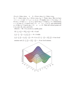
© Copyright 2026