
Viewing - ResearchGate
Time-Space Lower Bounds
for Undirected and
Directed ST -Connectivity
on JAG Models
by
Je A. Edmonds
A thesis submitted in conformity with the requirements
for the degree of Doctor of Philosophy
Graduate Department of Computer Science
University of Toronto
c Je Edmonds 1993
Abstract { Time-space lower bounds
for undirected and directed
st-connectivity on JAG models
Je A. Edmonds
Doctor of Philosophy 1993
Department of Computer Science
University of Toronto
Directed and undirected st-connectivity are important problems in computing. There are algorithms for the undirected case that use O (n) time and algorithms that use O (log n) space. The
rst result of this thesis proves that, in a very natural structured model, the JAG (Jumping Automata for Graphs), these upper bounds are not simultaneously achievable. This uses new entropy
techniques to prove tight bounds on a game involving a helper and a player that models a computation having precomputed information about the input stored in
its bounded
1 space. The second
1
2
result proves that a JAG requires a time-space tradeo of T S 2 mn 2 to compute directed
st-connectivity. The third result proves a time-space tradeo of T S 13 2 m 32 n 23 on a version
of the JAG model that is considerably more powerful and general than the usual JAG.
i
Acknowledgments
There are many people I wish to thank for helping me along the path from s to t. There were
those who held my hand while I walked the treacherous edges from idea to idea and bug to bug.
I am also indebted to those who helped me make sure that my ideas changed state from thought
to written form in a way that insured they were accepted rather than rejected. As I jumped from
deadline to deadline, there were always people who insured that I cleared the hurdles and who gave
me the support I needed to prepare for the next leap. Faith Fich, my advisor, provided the perfect
balance between directing my path and leaving me to take a random walk through the undirected
graph of research.
Courses and research groups were important in providing the necessary supplies for my trip.
They helped me learn about new papers, hear about the research of my peers, and gave me opportunities to share my own work. Some of my favorite courses were combinatorial methods by Faith
and Mauricio Karchmer, logic and non-standard numbers by Russell Impagliazzo and Steve Cook,
graph theory by Derek Corneil, distributed systems by Vassos Hadzilacos, and complexity by Al
Borodin. The research groups that most inuenced me were graph theory led by Derek Corneil,
NC2 led by Mauricio Karchmer, ordinals and graph minors led by Arvind Gupta, the probabilistic
method led by Hisao Tamaki, and complexity theory led by Al Borodin. The breadth requirements
were important as well. Some of them were actually interesting and taking them with Gara Pruesse
made them all the more enjoyable. Especially, the beer afterwards.
When I was traversing some of those edges during my mathematical odyssey, there were
many people who provided valuable support. Russell Impagliazzo, Arvind Gupta, Toni Pitassi,
Hisao Tamaki, Tino Tamon, and Chung Keung Poon were kind enough to listen to my ideas and
help me along. Some of my best work was also done jointly with these same people. Hisao, Tino,
C.K. and Russell were particularly helpful in providing me with information from the mathematical
literature that I wasn't as well versed in as I should have been. Al Borodin, Charlie Racko and
Steve Cook helped me by hitting my bugs with a y swatter. And of course, a great deal of thanks
goes to Faith Fich for treating me as a peer and for always being excited to discuss research.
I will always be grateful to those who helped me convert my research to understandable
English. Faith Fich was my most devoted critic and English teacher and spent much of her time
beating my writing into shape and combing out the typos. Since criticism is often hard to hear,
I sometimes relied on Jeannine St. Jacques to help put it into perspective. Many proof readers
were also crucial in revising my work. In addition to Faith Fich, I would like to thank Toni Pitassi,
Naomi Nishi, Jennifer Edmonds, Miriam Zachariah, Paul Beame, and some unknown referees who
were very hard working. I was also saved many times by Steven Bellantoni, Eric Schenk, and Ken
Lalonde when I was lost with Unix and Latex.
There were many people who provided the emotional support I needed to continue my journey.
ii
Faith Fich, Russell Impagliazzo, and Arvind Gupta, who had already become successful researchers,
often reassured me when I despaired about my own success. Faith was always there for me with
motherly love. Through out the years, Al too gave many touching words of support that were greatly
appreciated. I thank Derek Corneil, Arvind Gupta, Faith Fich, Steven Rudich, and Pat Dymond
for arranging for me to give talks outside of U. of T. which provided me with some of the exposure
and experience I needed. Martha Hendricks lightened things up and provided distractions when I
was working too hard. Rick Wallace, Shirley Russ, Roland Mak, and Toni Pitassi were always by
my side to help me with ongoing emotional issues.
PhD students are responsible for more than their own research. As I learned to teach undergraduates, I found important role models in Jim Mc Innes, Peter Gibbons, and Faith Fich. Kathy
Yen, Teresa Miao, and Vicky Shum led me by the hand when I had administrative obligations.
I would be remiss if I did not mention a few others who helped me on my way. My father, Jack
Edmonds, deserves some of the credit for my introduction to mathematics. He continually kept me
interested in puzzles to ponder. My mother, Patricia Oertel, provided support and encouragement
as I made my way through public school and university. Baby Joshua was very obliging in keeping
me awake at night so that I could do research. He also provided a lots of joy and love. My wife
Miriam was a tremendous support in every way possible and one last thanks goes to Faith Fich for
being such a wonderful advisor.
iii
Contents
1 Introduction
1.1
1.2
1.3
1.4
1.5
JAGS, NNJAGs, and Branching Programs : : :
Time Space Tradeos : : : : : : : : : : : : : :
The st-Connectivity Problem : : : : : : : : : :
A History of Lower Bounds for st-Connectivity
The Contributions of the Thesis : : : : : : : : :
:
:
:
:
:
:
:
:
:
:
:
:
:
:
:
:
:
:
:
:
:
:
:
:
:
:
:
:
:
:
:
:
:
:
:
:
:
:
:
:
:
:
:
:
:
:
:
:
:
:
2 The Helper-Parity Game
2.1
2.2
2.3
2.4
2.5
2.6
2.7
The Denition of the Game : : : : : : : : : : : : : : : : : : : : :
Viewing the Helper's Message as Random Bits : : : : : : : : : :
The Existence of a Helper-Parity Protocol : : : : : : : : : : : :
The r=2b Lower Bound : : : : : : : : : : : : : : : : : : : : : :
The (2 ? ) Lower Bound Using Probabilistic Techniques : : : : :
A (2 ? ) Lower Bound Using Entropy for a Restricted Ordering
A Simpler Version of the Helper-Parity Game : : : : : : : : : : :
3 Undirected st-Connectivity on a Helper-JAG
3.1
3.2
3.3
3.4
3.5
3.6
3.7
3.8
Graph Traversal : : : : : : : : : : : : : : : : : :
The Helper JAG : : : : : : : : : : : : : : : : : :
A Fly Swatter Graph : : : : : : : : : : : : : : : :
The Helper and a Line of Fly Swatter Graphs : :
The Recursive Fly Swatter Graphs : : : : : : : :
The Time, Pebbles, and Cost used at Level l : :
Reducing the Helper Parity Game to st-Traversal
The Formal Proof : : : : : : : : : : : : : : : : :
4 Directed st-Connectivity on a JAG
:
:
:
:
:
:
:
:
:
:
:
:
:
:
:
:
:
:
:
:
:
:
:
:
:
:
:
:
:
:
:
:
:
:
:
:
:
:
:
:
:
:
:
:
:
:
:
:
:
:
:
:
:
:
:
:
:
:
:
:
:
:
:
:
:
:
:
:
:
:
:
:
:
:
:
:
:
:
:
:
:
:
:
:
:
:
:
:
:
:
:
:
:
:
:
:
:
:
:
:
:
:
:
:
:
:
:
:
:
:
:
:
:
:
:
:
:
:
:
:
:
:
:
:
:
:
:
:
:
:
:
:
:
:
:
:
:
:
:
:
:
:
:
:
:
:
:
:
:
:
:
:
:
:
:
:
:
:
:
:
:
:
:
:
:
:
:
:
:
:
:
:
:
:
:
:
:
:
:
:
:
:
:
:
:
:
:
:
:
:
:
:
:
:
:
:
:
:
:
:
:
:
:
:
:
:
:
:
:
:
:
:
:
:
:
:
:
:
:
:
:
:
:
:
:
:
:
:
:
:
:
:
:
:
:
:
:
:
:
:
:
:
:
:
:
:
:
:
:
:
:
:
:
:
:
:
:
:
:
:
:
:
:
:
:
:
:
:
:
:
:
:
:
:
:
:
:
:
:
:
:
:
:
:
:
:
:
:
:
:
:
:
1
1
7
8
9
10
11
12
13
15
16
17
18
23
27
28
30
31
33
33
34
35
41
43
iv
4.1 Comb Graphs : : : : : : : : : : : : : : : : : : : : : : : : : : : : : : : : : : : : : : : : 43
4.2 JAGs with Many States : : : : : : : : : : : : : : : : : : : : : : : : : : : : : : : : : : 44
5 Directed st-Connectivity on a NNJAG
5.1
5.2
5.3
5.4
5.5
5.6
5.7
5.8
A Probabilistic NNJAG with One Sided Error : : : : : : : : : : : : :
The Probability Distribution D on Comb Graphs : : : : : : : : : : :
The Denition of Progress : : : : : : : : : : : : : : : : : : : : : : : :
Converting an NNJAG into a Branching Program : : : : : : : : : : :
The Framework for Proving Lower Bounds on Branching Programs :
A Probabilistic NNJAG with Two Sided Error : : : : : : : : : : : :
Trials : : : : : : : : : : : : : : : : : : : : : : : : : : : : : : : : : : :
The Probability of Finding a Hard Tooth : : : : : : : : : : : : : : :
:
:
:
:
:
:
:
:
:
:
:
:
:
:
:
:
:
:
:
:
:
:
:
:
:
:
:
:
:
:
:
:
:
:
:
:
:
:
:
:
:
:
:
:
:
:
:
:
:
:
:
:
:
:
:
:
:
:
:
:
:
:
:
:
:
:
:
:
:
:
:
:
47
47
49
49
50
51
52
55
56
6 Future Work
60
7 Glossary
63
6.1 Undirected Graphs : : : : : : : : : : : : : : : : : : : : : : : : : : : : : : : : : : : : : 60
6.2 Directed Graphs : : : : : : : : : : : : : : : : : : : : : : : : : : : : : : : : : : : : : : 61
v
Chapter 1
Introduction
This thesis proves lower bounds on the time-space tradeos for computing undirected and directed st-connectivity on the JAG and related models of computation. This introductory chapter
introduces the models of computation considered, gives a brief history of time-space tradeos, summarizes the known upper and lower bounds for st-connectivity, and outlines the contributions of
the thesis.
1.1 JAGS, NNJAGs, and Branching Programs
Many dierent models of computation are used in computer science. These abstract the crucial
features of a machine and allow theoreticians, programmers, and architecture designers to communicate in succinct ways. Another motivation for dening models is to be able to prove lower
bounds. A long term goal is to be able to prove lower bounds on the Random Access Machines
(RAM), because this is the abstraction that best models the computers used in practice. However,
this goal remains elusive.
In order to make the task of proving lower bounds easier, models are dened that are in some
ways more restricted than the RAM and in some ways are less restricted. One way of restricting
the model is to restrict the order in which it is allowed to access the input. Another way is to not
allow the actions of the model to depend on the aspects of the input that have to do with the input
representation and not on the output of the computational task at hand. The usual justication
for restricting the model in these ways is that it seems natural and that most known algorithms
for the given problem adhere to the restrictions.
One way to strengthen a model is to dene the model's internal workspace in such a way that
no assumptions are made about how the space is managed. Another way to strengthen the model
is to add to its instruction set; in the extreme, allow the model to compute any function of the
known information in one time step.
This thesis is particularly interested in two models; JAGs and NNJAGs, and is indirectly
interested in branching programs. These models and some closely related models are dened below.
In Figure 1.1, the relative strengths in terms of direct simulations between these models, the RAM
and the Turing machine are depicted.
The (r-way) branching program [BC82] is the most general and unstructured model
1
BP
RAM
Strong Jumping
TM
NN-JAG
NN-JAG
Comparison
BP
JAG
Figure 1.1: Models of Computation
of sequential computation and is at least as powerful as all reasonable models of computation.
Depending on the current state, one of the input variables is selected and its value is queried.
Based on this value, the state changes. These state transitions are represented by a directed acyclic
rooted graph with out-degree r, where r is the maximum number of dierent values possible for an
input variable. Each node of this graph represents a possible state that the model might be in and
is labeled with the input variable that is queried in this state. The edges emanating out of the node
are labeled with the possible values of the queried variable and the adjacent nodes indicate the
results of the corresponding state transitions. In order to indicate the outcome of the computation,
each sink node is labeled with either accept or reject. A computation for an input consists of
starting at the root of the branching program and following a computation path through the
program as explained above, until an accept or reject sink node is reached. The time TG is the
length of the computation path for input G. The space S is formally the logarithm of the number of
nodes in the branching program. Equivalently, it can be viewed as the number of bits of workspace
required to specify the current state. The branching program is said to be leveled if the nodes can
be assigned levels so that the root has level 0 and all edges go from one level to the next.
The branching program model is more powerful than the RAM model in the two ways mentioned above. Assumptions are made about how the RAM manages its workspace. Specically, the
workspace is broken into many small squares and the RAM is only allowed to alter one of these
squares at a time. What may be more signicant is that, during a particular time step, the RAM's
next action is allowed to depend only on a nite state control together with the contents of only a
few of these input squares. In contrast, the state of the branching program species the contents
of the entire workspace. A branching program is able to alter the entire workspace in one time
step by means of the appropriate state transition and its next action can depend on its new state
in an arbitrary way. Because any transition is allowed, no assumption is made about the way the
model's workspace is managed.
A RAM is also restricted in comparison to a branching program because it has a limited
instruction set. A RAM can compute the sum or the product of the contents of two squares in
one step, but is not, for example, able to quickly factor these numbers. A branching program does
not have this restriction. Its state transition function can be dened arbitrarily and non-uniformly.
Hence, in one time step, it can compute any function of the known information in a manner that
amounts to a table lookup.
Although in many ways unrealistic, the advantage of proving lower bounds on the more
2
powerful branching program model is that we gain the understanding of what features of the
computational problem really are responsible for its diculty. Another benet is that a number of
proof techniques have been developed for the branching program model, whereas we have few tools
to take advantage of the fact that RAM has a restricted instruction set or that it can change only
one bit of its workspace at a time. Besides, any lower bounds for the branching program apply to
the RAM.
Proving lower bounds for decision problems on either the branching program model or the
RAM is beyond the reach of current techniques. Hence, restricted models of computation are
considered. One model that has been a successful tool for understanding the complexity of graph
connectivity is the \jumping automaton for graphs" (JAG) model introduced by Cook and Racko
[CR80]. This model restricts the manner in which it is allowed to access the input and in the type
of information about the input that it is allowed to access. In addition, some of its workspace is
structured to contain only a certain type of information. As well, its basic operations are based on
the structure of the graph, as opposed to being based on the bits in the graph's encoding [Bo82].
Hence, it is referred to as a \structured" model of computation. The JAG model has a set of
pebbles representing node names that a structured algorithm might record in its workspace. They
are useful for marking certain nodes temporarily, so that it can be recognized when other pebbles
reach them.
1
3
s
1
2
1
1
2
1 2
3 1 2
2 3
2
2 1
1 3
1 t
2
Current
State
Figure 1.2: The JAG model for undirected graphs
Ajacency List
v1
v2
v3
v4
deg = 3 : v3 , v1 , v5
deg = 2 : v4 , v3
deg = 4 : v2 , v1 , v4 , v9
deg = 2 : v1 , v3
Current
State
names of p nodes
Figure 1.3: The structured allocation of the workspace that the JAG models
The
JAG [CR80] is a nite automaton with p distinguishable pebbles and q states. The
3
space charged to the model is dened to be S = p log2 n + log2 q . This is because it requires log2 n
bits to store which of the n nodes a pebble is on and log2 q bits to record the current state.
The input to this JAG model is a graph with n nodes, m edges, and two distinguished nodes
s and t. The input graph is directed or undirected depending on whether directed or undirected
st-connectivity is being considered. For each node v, there is a labeling of the out-going edges with
the numbers from 1 to the out-degree of the node. (If the edge is undirected, it can receive two
dierent labels at its two endpoints.) One of the pebbles is initially placed on the distinguished
node t and the other p ? 1 are placed on s. The initial state is Q0.
Each time step, the automaton is allowed an arbitrary non-uniform state transition similar
to that of a branching program. It also does one of the following two things. It either selects some
pebble P 2 [1::p] and some label l and walks P along the edge with label l or it selects two pebbles
P; P 0 2 [1::p] and jumps P to the node occupied by P 0 . (For directed graphs, the pebbles may be
walked in the direction of an edge, but not in the reverse direction.)
What the JAG chooses to do each time step is only allowed to depend on specic parts of
the current machine conguration. Specically, its actions are able to depend on the current state,
which pebbles are on the same nodes, which pebbles are on the distinguished nodes s and t, and
the out-degrees of the nodes containing pebbles1 . (For directed graphs, the model has no direct
access to the in-degrees of the nodes.)
A JAG that solves undirected st-connectivity enters an accepting state if there is an undirected
path between s and t in the input graph and enters a rejecting state if there is no such path.
Similarly, a JAG that solves directed st-connectivity enters an accepting state if and only if there
is a directed path from s to t.
Now that it has been specied what the JAG model is allowed to do, I will make it clearer
what it has not been allowed to do. It is, in fact, restricted in the two ways mentioned at the
beginning of this section.
Like the Turing machine, the JAG model is restricted in the order in which it is allowed to
access its input. The Turing machine is only allowed to move its input heads one square to the
right or one to the left in a single step. The JAG is only allowed to \walk" and \jump" its pebbles.
For the task of graph st-connectivity, accessing the input in an order constrained by the Turing
machine's tape does not seem to be natural. In fact, such a restriction would likely increase the
complexity of the problem by a factor of O (n). 2 In contrast, \walking" pebbles along the edges
of the input graph does seem to be natural to the computational problem at hand. After all, the
model can know that s is connected to t simply by \walking" a pebble from s to t.
Being able to \jump" a pebble directly to the node containing another pebble also adds a
great deal of power to the JAG model that the Turing machine does not have. From lower bounds
on JAGs that are not allowed to jump (WAGs) [BRT92, BBRRT90], it can be concluded that
jumping increases the model's power signicantly, because the model is able to quickly concentrate
its limited pebble resources in the subgraph it is currently working on.
At rst, it might seem unnatural that the JAG model for directed graphs is not allowed to
1 The graphs
in [CR80] are d-regular for some xed degree. I am allowing the input to be more general. The JAG
is told the out-degree of the nodes containing pebbles so that it knows which labels l it can choose for walking a
pebble. The distinction is of greater importance when the model is being charged for the computation time.
2 [CR80] charged the model only for space. I am charging the model for time as well. Hence, these factors are
important.
4
access the in-degree or allowed to walk in the reverse direction along an edge. However, suppose the
input is stored by listing, for each node, the out-degree followed by the out-adjacency list. Then,
even a RAM, would not be able to learn the in-adjacency list of a node without scanning the entire
input3 . Hence, not allowing the JAG to walk pebbles backwards along directed edges is reasonable
and natural.
Even when the order in which the model is allowed to access its input is restricted, proving
lower bounds for decision problems like st-connectivity is hard. One reason is that a general model
of computation is able to perform weird tasks and store arbitrary information. Hence, it is dicult
for us to judge, for each of the possible states that the model might be in, how much progress has
been made towards solving the given problem. By restricting the model again so that it is only able
to learn or store \structured" information about the input, it is then possible to dene a measure
of progress.
More precisely, any input representation of a graph that is written as a list of values must
impose \names" on the nodes of the graph. With these names, a general model of computation is
able to do strange things like taking their bitwise parity and then changing its actions based on
the values obtained. In contrast, the JAG is not allowed to do things which seem to be unnatural.
This restriction can viewed as a restriction on the instruction set of the JAG or, equivalently, as
a change in the way that the input is represented. The input graph can be considered to be as
an abstract object, in which the nodes other than s and t do not have names. The actions of the
JAG do not depend on the names of these nodes. Eectively, this means that the actions of the
JAG are not allowed to depend on which nodes the pebbles are on, but only on which pebbles are
on the same nodes. Note that the answer to a problem instance and hence the nal outcome of a
computation does not depend on the names of the non-distinguished nodes.
The JAG is not the only model that is restricted in how it can react to its input. The comparison based branching program is another example. In this model, a step consists of comparing two
inputs variables and changing state based on which is larger. Hence, the actions of a comparison
based branching program are allowed to depend on the permutation describing the relative ordering of the input variables, but not on the actual values of these variables. Similarly, an arithmetic
circuit model is able to add, subtract, and multiply the values of certain input variables, but the
choice of operations and the variables cannot depend on the actual values that variables have.
Despite the fact that the JAG is restricted in two signicant ways, the JAG is not a weak model
of computation. To begin with, it is not strictly weaker than the RAM, because like a branching
program, it allows arbitrary non-uniform state transitions. More importantly, it is general enough
so that most known algorithms for graph connectivity can be implemented on it. See Section 1.3
for some upper bounds. Furthermore, Beame, Borodin, Raghavan, Ruzzo, and Tompa [BBRRT90]
give a reduction that transforms any O (s) space Turing machine algorithm for any undirected
graph problem to run on a O (s) space JAG within a polynomial factor as fast. Hence, a lower
bound for the JAG
? translates to a lower bound for a Turing machine. However, this is not helpful
here because n2 time bounds for the JAG are too small as compared to the overhead incurred
by this reduction.
There has been a great amount of success in proving lower bounds on the JAG model. Poon
[Po93b] has taken this work another step further by introducing another model that is considerably
3 An
interesting related problem is the following. The input is a set of n pointers forming a set of linked lists of
length l and the last node of one of the lists. The output is the head of the list whose last node has been specied. I
conjecture that a RAM with O (log n) space would require (ln) time.
5
less restricted. The model is referred to as the node named jumping automaton for graphs (NNJAG).
The initial motivation for dening this model was to overcome an apparent weakness of the JAG:
namely, on the JAG, it does not seem possible to implement Immerman's non-deterministic O (log n)
space algorithm for detecting that a graph is not st-connected. However, Poon can do so on an
NNJAG.
The NNJAG is an extension of the JAG, with the additional feature that it can execute
dierent actions based on which nodes the pebbles are on. This feature makes the NNJAG a
considerably more general model of computation than the JAG. The NNJAG is able to store
arbitrary unstructured information about the names of the nodes by transferring the information
that is stored in the \pebble workspace" into the \state workspace". This is done by having the
state transition depend on the names of the nodes containing pebbles.
If the NNJAG was to be able to access its input in an arbitrary order, then the model would
be equivalent to the branching program model. However, it is not. Although it can store any
information in its state, it can only gain new information about the input graph by means of its
pebbles. In addition, even if the model knows the name of a particular node, it is only allowed to
\jump" a pebble there if another pebble is already there and to get a pebble there initially, it must
\walk".
The NNJAG seems incomparable to the Turing machine, because they are allowed to access
their inputs in dierent orders. Savitch introduced a new operation, strong jumping, to the
JAG model [Sa73]. Strong jumping is the ability to move any pebble from a node to the next
higher numbered node, for some ordering of the nodes. Such an operation seems to be comparable
to jumping a pebble to an arbitrary node of the graph, because the nodes can be placed by an
adversary in an arbitrary order. On the other hand, with this additional power, the NNJAG model
is strictly more powerful than the Turing machine model by direct simulation. Because the NNJAG
lacks this ability, it is not able scan to the entire input in linear time. In fact, pebbles are never
able to reach components of the input graph that do not initially contain pebbles. For solving
st-connectivity, it does not seem that the model could gain useful information by doing this, but
this restriction does mean that the JAG and the NNJAG are not considered generals model of
computation. At present, we are unable to remove this restriction on the model, because it is this
feature that enables us to prove lower bounds for JAGs. Recall that a diculty in proving lower
bounds is dening a measure of the amount of progress that a computation has done. For the
NNJAG model, this problem is solved by dening progress in terms of how much of the graph the
model has accessed so far.
All the above mentioned models, the branching program, the JAG, and the NNJAG are
deterministic. Probabilistic versions of these models can be dened quite simply. For every random
string R 2 f0; 1g, the model will have a separate algorithm, with disjoint states. At the beginning
of the computation a random R 2 f0; 1g is chosen. Then the computation proceeds as before with
the selected algorithm.
The space of a probabilistic JAG, NNJAG, or branching program is dened to be the maximum of the space used by each of the separate algorithms. This eectively provides the model
with jRj bits of read only workspace which contains R and which can be accessed in its entirety
every time step.
As long as the model has enough space to store the time step, i.e. S log T , this way of
representing probabilism is stronger than supplying the model with a few random bits each time
6
step4 . In this case, the time step can be used as a pointer into R. Yao uses this same denition
of randomization [Ya77]. However, for upper bounds this denition is unrealistic. A non-uniform
algorithm for one value of n can be specied in polynomial size by giving the circuit. However,
specifying such a random algorithm requires a non-uniform circuit for each random string.
A probabilistic algorithm is said to allow zero-sided error if the correct answer must always
be produced; however, the running time may depend on the choice of the random string R. A
probabilistic algorithm is said to allow one-sided error if for every input not in the language,
the correct answer is given, but for inputs in the language the incorrect answer may be given with
some bounded probability. A probabilistic algorithm is said
to allow two-sided error if for every
input, it may give the incorrect answer with probability 12 ? .
We have now dened models of computation that are both non-uniform and probabilistic. In
many circumstances, this is redundant. Adleman tells us how to convert a probabilistic algorithm
into a non-uniform deterministic algorithm [Ad78]. He does this by proving that, for every probabilistic algorithm, there exists a set of O (n) random strings R, such that for every input, one of the
random strings gives the correct answer. The non-uniform algorithm is to simply deterministically
run the probabilistic algorithm for each of these choices of R. An eect of this reduction is that a
lower bound on a non-uniform deterministic model applies for free to the probabilistic version of the
model. The only diculty
is that, because the reduction blows up the time by a factor of O (n),
?
2
a lower bound of n on the non-uniform deterministic model would say nothing non-trivial
about the probabilistic model. Therefore, there is value to proving lower bounds on non-uniform
probabilistic models of computation. Clearly, such a bound applies to uniform probabilistic models
as well.
Yao compares worst case probabilistic algorithms and average case deterministic algorithms
[Ya77]. He proves that there exists a probabilistic algorithm whose expected running time on the
worst case input is T if for every distribution on inputs, there exists a deterministic algorithm
whose average running time weighted by the input distribution is T . This means that if there is
not a probabilistic algorithm, then there exists a distribution for which there is no algorithm that
is fast on average with respect to this distribution. This thesis will strengthen the lower bound
further by specifying a specic natural input distribution for which the average time must be large.
In fact, this thesis considers both of these settings at the same time, i.e. average case probabilistic
algorithms. Given Yao's result, this might be excessive, but it is helpful for forming additional
intuition.
The lower bounds proved are on probabilistic JAGs for undirected graphs, JAGs for directed
graphs, and probabilistic NNJAGs for directed graphs.
1.2 Time Space Tradeos
Proving time-space tradeos is one of the more classical issues in complexity theory. For some
computational problems it is possible to obtain a whole spectrum of algorithms within which one
can trade the time requirements with the storage requirements. In these cases, the most meaningful
4 If the space is less than this, then the random bits cannot be chosen initially, because the model cannot remember
them. Beame et al. [BBRRT90] proved that a deterministic WAG with pq = (n) traversing 2-regular graphs have
innite worst case time. Hence, with the random bits provided at the beginning of the computation, the expected
time would be innite. However, a probabilistic WAG can easily traverse such a graph in expected n2 time.
7
bounds say something about time and space simultaneously.
Cobham [Co66] established the rst time-space tradeo. The model used was a one tape
Turing Machine. Tompa [Tm80] established a number of time-space tradeos for both the Boolean
and the arithmetic circuit models.
Borodin, Fischer, Kirkpatrick, Lynch, and Tompa [BFKLT81] introduced a framework that
has been extremely successful in proving lower bounds on the time-space tradeos? for branching
programs. Using this framework, they prove the near optimal bound of T S 2 n2 for sorting
on comparison based branching programs. Borodin and Cook [BC82] strengthened this result
signicantly by proving the rst non-trivial time-space tradeo lower bound for a completely general
and
model of computation, the r-way branching program. They showed that
T S 2
nunrestricted
?
2 2
2
log n for sorting n integers in the range [1::n ]. Beame [Be91] improved this to n . These
same techniques were also used to prove lower bounds for a number of algebraic problems such as
the FFT, matrix-vector product, and integer and matrix multiplication [Ye84, Ab86, BNS89].
Each of these lower bounds relies heavily on the fact that the computation requires many
values to be output, in order to establish a measure of progress. For decision problems this method
does not work. Borodin, Fich, Meyer auf der Heide, Upfal, and Wigderson [BFMUW87] dene a
new measure of progress and
3 provea lower bound on the time-space tradeo for a decision problem.
They proved T S 2 n 2 log n for determining element distinctness. This was then improved
? to T S 2 n2? by Yao [Ya88]. They were not, however, able to prove this bound for a general
model of computation, but only for the comparison based branching program.
1.3 The st-Connectivity Problem
Graph connectivity is an important problem, both practically and theoretically. Practically, it
is a basic subroutine for many graph theoretic computations. It is used in solving network ow
optimization problems, such as project scheduling and the matching of people to jobs. Theorem
proving can be viewed as nding a logical path from the assumptions to the conclusion. Graph
connectivity is also important for computer networks and search problems. Theoretically, it has
been studied extensively in a number of settings. Because the undirected version of the problem
is complete for symmetric log-space and the directed version is complete for non-deterministic
log-space, they are natural problems for studying these classes. The study of random walks on
undirected graphs and deterministic universal traversal sequences has made the problem relevant to
the issue of probabilism. In addition, the undirected version was used by Karchmer and Wigderson
to separate monotone NC1 from NC2. The importance of these problems is discussed in more
detail in Wigderson's beautiful survey [Wi92].
The fastest algorithms for undirected graph st-connectivity are depth-rst and breadth-rst
search [Tar72]. These use linear time, i.e. O (m + n) for an n node, m edge graph. However, they
require (n) space on a RAM.
Alternatively, this problem can be solved probabilistically using random walks. The expected time to traverse any component of the graph is only (mn) and uses only O (log n) space
[AKLLR79]. More generally, Broder et al. [BKRU89] have exhibited a family of probabilistic algorithms that achieves a tradeo of S T 2 m2 logO(1) n between space and time. This has been
improved to S T 2 m1:5n:5 logO(1) n [BF93]. A long term goal is to prove a matching lower bound.
8
Deterministic non-uniform algorithms for st-connectivity can be constructed using Universal
traversal sequence. The algorithm uses? a single
the connected components
\pebble" tototraverse
of the graph. Sequences of length O n4 log?n are proved
exist
[CRRST89,
KLNS89]. This
proves the existence of O (log n) space and O n4 log n time algorithms. Nisan provides an explicit
constructions of a universal traversal sequences
using pseudo-random generators. This gives a
deterministic uniform algorithm using O log2 n space and nO(1) time [Ni92]. Finally, Nisan, Sze
meredi, and Wigderson describe and a deterministic uniform algorithm that uses only O log1:5 n
1:5
space [NSW92]. The time for this algorithm, however, is 2O(log n) .
Directed st-connectivity has the same complexity as undirected st-connectivity when there
is ample space. Specically, the linear time, linear space, depth rst search algorithm works ne.
However, the known algorithms for the directed problem require considerably moretime when
the
space allocated to the model is bounded. Savitch's algorithm [Sa70] uses only O log2 n space,
but requires 2O(log2 n) time. It is only recently that a polynomial time, sub-linear O 2pnlog n space
algorithm was found for directed st-connectivity [BBRS92].
Section 1.1 stated that the JAG model is general enough so that most known algorithms
for graph connectivity can be implemented on it. I will now be more specic. It can perform
depth-rst or breadth-rst search. It avoids cycling by leaving a pebble on each node when it
rst visits it. This uses O (n log n) space. As well, because it is a non-uniform
? model,
the JAG is
able to solve st-connectivity for undirected graphs in O (log n) space and O n4 log n time using a
universal traversal sequence [CRRST89, KLNS89]. For directed graphs, Cook and Racko [CR80]
show that the JAG model
is powerful enough to execute an adaptation of Savitch's algorithm [Sa70]
2
which uses O log n space. Poon [Po93a] shows that Barnes et al.'s [BBRS92] sub-linear space,
polynomial time algorithm for directed st-connectivity runs on a JAG as well.
1.4 A History of Lower Bounds for st-Connectivity
A number of space lower bounds have been obtained (even when an unbounded amount
of time
2
is allowed). Cook and Racko [CR80] prove a lower bound of log n= log log n on the space
required for a JAG to compute directed st-connectivity. This has been extended to randomized
JAGs by Berman and Simon [BS83] (for T 2 2logO(1) n ). Recently, Poon [Po93b] has extended this
result again to the powerful probabilistic NNJAG model.
For undirected graph st-connectivity, Cook and Racko [CR80] prove that pq 2 ! (1) and
Beame et al. [BBRRT90] prove that if the pebbles are not allowed to jump, then pq 2 (n) even
for simple 2-regular graphs. These proofs for undirected graphs show that, with a sub-linear number
of states, the model goes into an innite loop. (This method does not work when there are at least
a linear number of states, because then the JAG is able to count the time steps.)
Lower bounds on the tradeo between the number of pebbles p used and the amount of time
needed for undirected graph st-connectivity have also been obtained. These results are particularly
strong, because they do not depend on the number of states q . For example, a universal traversal
sequence is simply a JAG with an unlimited number of states, but only one pebble. Borodin,
? Ruzzo, and Tompa [BRT92] prove that on this model, undirected st-connectivity requires m2
time where the graph has degree 3 d 31 n ? 2. Beame, Borodin, Raghavan, Ruzzo, and Tompa
9
?
[BBRRT90] extend this to n2 =p time for p pebbles on 3-regular graphs with the restriction that
all but one pebble are unmovable (after being initially placed throughout the graph). Thus, for
this very weak version of the model, a quadratic lower bound on timespace has been achieved.
Beame et al. [BBRRT90] also prove that there is a family of 3p-regular
n undirected graphs for which
st-connectivity with p 2 o (n) pebbles requires time m log p , when the pebbles are unable
to jump.
1.5 The Contributions of the Thesis
This thesis proves time-space tradeos for both undirected and directed st-connectivity. The rst
result, presented in Chapter 3 proves the strongest known bound for undirected st-connectivity.log The
n
result is that the expected time to solve undirected
nO2(1)
( log log n ),
log n st -connectivity on a JAG is at least log
n . This
as long as the number of pebbles p 2 O log log n and the number of states q 2 2
result improves upon at least one of the previous results in at least ve ways: the lower bound
on time is larger, all pebbles are allowed to jump, the degree of the graphs considered is only
three, it applies to an average case input instead of just the worst case input, and probabilistic
algorithms are allowed.
This result is obtained by reducing the st-connectivity problem to the problem of traversing
from s to t and then reducing this problem to a two player game. Chapter 2 proves tight bounds for
this game. The game is referred to as the helper-parity game and is designed to mirror a key aspect
of time-space tradeos. When the space is bounded, the computation cannot store the results to all
the previously computed subproblems and hence must recompute them over and over again. The
diculty in proving lower bounds is that we must assume that earlier stages of the computation
communicate partial information about the subproblem via the bounded workspace. The question
then is how helpful this information can be in decreasing the time to recompute the subproblem by
the later stages. This is modeled in the helper-parity game by having the helper communicate the
stored information to the player at the beginning of the player's computation. Upper and lower
bounds are provided giving the tradeo between the amount of information that the helper provides
and the time for the player's computation.
Chapter 4 proves the even stronger lower bound of T S 21 2 mn 21 , but for the more
dicult computational problem of directed st-connectivity. This is the rst time-space tradeo
where the pebbles are able to jump and their number is unrestricted. Note, as well, that the time
bound matches the upper bound of O (m + n) when the amount of available space increases to n.
Another interesting feature of the result is that it does not count the number of states as part of
the space and hence applies even when the JAG has an arbitrarily large number of states. It had
been assumed that the time to compute st-connectivity on a JAG became linear as the number of
states increases.
Chapter 5 then proves a weaker bound of T S 31 2 m 23 n 23 on the same family of graphs,
but on the more powerful probabilistic NNJAG model. Very dierent techniques are required to
accomplish this. The general framework is the one outlined in Section 1.2.
The last chapter describes some current work and open problems.
10
Chapter 2
The Helper-Parity Game
The essential reason that tradeos arise between the time and the space required to solve a problem
is that when the space is bounded the computation cannot store the results to all the previously
computed subproblems and hence must recompute them over and over again. The diculty in
proving lower bounds is that only in the rst encounter with a subproblem is the computation
completely without knowledge about the solution. We must assume that the earlier stages of the
computation communicate partial information about the subproblem via the bound workspace.
This chapter characterizes this problem in terms of a game referred to the helper-parity game. The
helper in the game communicates to the player the information that would be stored in the bounded
workspace. The player then uses this information to help in his computation. Upper and lower
bounds are provided in this chapter, giving the tradeo between the amount of information that
the helper provides and the time for the player's computation.
The hope was that requiring the player to solve multiple instances of the problem would make
proving time-space tradeos easier. Because the space is bounded, the number of bits of information
that the helper is allowed to give the player is bounded. Even if this is enough information for
the player to quickly solve one instance of the problem, the hope was that the helper would not
be able to encode the relevant information about many instances into the same few bits. What
was expected was that if the number of game instances doubles, then the number of bits of help
would need to double as well in order for the complexity per instance to remain constant. This,
however, is not the case. If the same bits of help are given for an arbitrarily large number of
instances, then the complexity of each instance can drop as eectively as if this many bits of help
were given independently to each of the instances. It is surprising that enough information about
so many game instances can be encoded into so few bits. This appears to contradict Shannon's
laws concerning the encoding of information.
This upper bound is best understood by not considering the message sent by the helper as
being information about the input, but as being random bits. With a few \random" bits, the worst
case complexity decreases to the point that it matches the expected complexity for a randomized
protocol, which is 2 questions per game instance. The upper and lower bounds on the number
of helper bits required match the work done by Impagliazzo and Zuckerman [IZ89] on recycling
random bits.
For the purpose of proving lower bounds on time-space tradeos these results are disappointing. Increasing the number of game instances does not help in the way we hoped. However, the
11
results are still useful. Though, achieving 2 questions per game instance requires very few help
bits, a lot of help bits are required to decrease the number of required questions below this number.
Furthermore, this 2 (actually a 1.5) is sucient of provide the lower bound in Chapter 3.
2.1 The Denition of the Game
The task of one game instance is to nd a subset of the indexes on which the input vector has
odd parity. This idea was introduced by Borodin, Ruzzo, and Tompa [BRT92] for the purpose of
proving lower bounds for st-connectivity. The basic idea is that the input graph has two identical
halves connected by r switchable edges. A vector 2 f0; 1gr species which of the switchable
edges have both ends within the same half of the graph and which span from one half to the other.
Traversing from distinguished node s to distinguished node t requires traversing a pebble from one
half of the graph to the other. After a pebble traverses a sequence of switchable edges, which half
of the graph the pebble is contained in is determined by the parity of the corresponding bits of .
The JAG computation on this graph is modeled by a parity game. The following is a more complex
game. A version of it is used in Chapter 3.
The helper-parity game with d game instances is dened as follows. There are two parties,
a player and a helper. The input consists of d non-zero r bit vectors 1 ; : : :; d 2 f0; 1gr?f0r g,
one for each of the d game instances. These are given to the helper. The helper sends b bits in
total about the d vectors. The player asks the helper parity questions. A parity question species
one of the game instances i 2 [1::d] and a subset of the indexes E [1::r]. The
answer to the
L
parity question is the parity of the input i at the indexes in this set, namely j 2E [i ]j . The
game is complete when the player has received an answer of 1 for each of the game instances. For
a particular input ~ , the complexity
of the game is the number of questions asked averaged over
P
1
the game instances, c~ = d i2[1::d] ch~ ;ii, where ch~ ;ii is the number of questions asked about the
ith game instance on input ~ . Both worst case and average case complexities are considered.
One instance of the helper-parity game can be solved using at most 2rb questions per game
instance as follows. Partition the set of input positions [1::r] into 2b blocks. The helper species
the rst non-zero block. The player asks for the value of each bit within the specied block. A
matching worst case complexity lower bound for this problem is easy to obtain.
For d game instances, one might at rst believe that the worst case number of questions per
r . The justication is that if the helper sends the same b bits to all of
game instance would be 2b=d
the game instances then on average only b=d of these bits would be about the ith game instance.
r questions about this instance. The helper and the
Therefore, the player would need to ask 2b=d
player, however, can do much better than this. The number of questions asked averaged over the
number of game instances satises
2r i
h
hr
i
max 2rb ; 2?O db + 2?r+1 Exp~ c~ max
+log
(
e
)+log
c
max
+
o
(1)
;
2+
o
(1)
:
2b
2b
~ ~
As long as the bound is more than 2, it does not depend on the number of game instances
d. Therefore, if we x the size of each game instance r, x the number of questions c asked by the
player per game instance, and increase the number of game instances d arbitrarily, then the number
of help bits b needed does not increase. Given that each player requires some \information" from
the helper \about" each game instance, this is surprising. The result 2rd also says that there is no
12
dierence between the helper independently sending b bits of help for each of the game instances
and requiring the helper to send the same b bits for each of the instances.
This chapter is structured as follows. Section 2.2 explains the connection between these
results and the work done by Impagliazzo and Zuckerman on recycling random bits [IZ89]. In this
light, the results are not as surprising. Section 2.3 proves that a protocol exists that achieves the
upper bound and Section 2.4 gives the simple 2rb lower bound. Section 2.5 presents a recent proof
by Rudich [R93] of the (2 ? ) lower bound. Section 2.6 proves my own (2 ? ) lower bound for
the problem under the restriction that the player must solve the game instance being worked on
before dynamically choosing the next game instance to work on. Both proofs are presented because
they use completely dierent proof techniques. My proof uses entropy to measure the amount of
information the helper's message contains \about" the input i to each game instance and then
examine how this message partitions the input domain. Rudich avoids the dependency between
the game instances caused by the helper's message by using the probabilistic method. Section 2.7
denes a simpler version of the helper-parity game. The st-connectivity lower bound in Chapter 3
could be proved using the original game, but the proof becomes much simpler when using this
simpler game. A tight lower bound is proved for this version of the game using my techniques.
Rudich's techniques could be used to get the same result.
2.2 Viewing the Helper's Message as Random Bits
The fact that the player need ask only maxf 2rb ; 2g questions per game instance may seem surprising.
However, if the game is viewed in the right way, it is not surprising at all. The incorrect way of
viewing the game is that the helper sends the player information about the input. With this view
the result is surprising, because Shannon proves that it requires d times as many bits to send a
message about d dierent independent objects. The correct way of viewing the game is that the
helper sends the player purely random bits. With this view the result is not surprising, because
Impagliazzo and Zuckerman [IZ89] prove that the player can recycle the random bits used in solving
one game instance so that the same random bits can be used to solve other game instances. To
understand this, we need to understand how random bits can help the player, understand how a
random protocol for the game can be converted into a deterministic protocol, and nally understand
how many random bits the helper must send the player.
With no helper bits, if the player asks his questions deterministically, then on the worst case
input, he must ask rd questions. However, if the helper sent the player random bits, then the player
could deterministically use these to choose random questions (from those that are linearly independent from those previously asked). With random questions, the expected number of questions per
a game instance is 2. This is because a random question has odd parity with probability 21 .
By the denition of the game, the helper is not able to send a random message, but must
send a xed message M (~ ) determined by the input ~ . However, this causes no problem for the
following reason. Suppose that there is exists a protocol in which the helper sends the players b
random bits and on every input ~ there is a non-zero probability that the player succeeds after
only c questions. It follows that for every input ~ , there exists a xed message M (~ ) for which the
player asks so few questions. Hence, a deterministic protocol could be dened that achieves this
same complexity by having the helper send this xed message M (~ ) on input ~ .
The question remaining is how many random bits a player needs. First consider one game
13
instance. With b random bits, the player can partition [1::r] into 2b blocks and ask for the values
of each of the bits of within the randomly specied block. Because the entire vector is nonzero, the specied block will be non-zero with a non-zero probability. In this case, the player will
succeed at getting an
answer with odd parity. The number of questions asked by the player is
r . Hence, b = log ? r random bits are needed to ensure that the player is able to succeed with
c
2b
non-zero probability after only c questions. Note that this is exactly the complexity of one game
instance when viewing the helper's message as containing information about the input. A savings
is obtained only when there are many game instances.
Impagliazzo and Zuckerman [IZ89] explain how performing an experiment might require lots
of random bits, but the entropy that it \uses" is much less. Their surprising result is that the
number of random bits needed for a series of d experiments is only the number of random bits
needed for one experiment plus the sum of the entropies that each of the other experiments uses.
The consequence of this for the helper-parity game is that if the player recycles the random bits it
obtains, then the helper need not send as many bits.
Although this technique decreases the number of helper bits needed, it does not completely
explain the amazing upper bound. Recall that the upper bounds says that as the number of game
instances increases arbitrarily, the number of helper bits does not need to increase at all. The
explanation is that we do not require each player to ask fewer than c questions about each game
instance. We only require that the total number of questions asked is less than cd. Because at
most 2 questions are likely to be asked, this will be the case for most inputs. The player is then
able to ask almost O (cd) questions about a few of the game instances and still keep the total
number of questions within the requirements. Ensuring that the maximum number of questions
asked about a particular instance is at most O (cd) requires far fewer random bits then ensuring
that the maximum is c. Therefore, as d increases, the number of random bits needed per game
instance decreases so that the total number remains xed.
Before proving that such a protocol exists, let us try to understand the Impagliazzo and
Zuckerman result better by considering a sightly dierent version of the helper-parity game. Instead
of requiring that the total number of questions asked be at most cd, let us consider requiring that
for each game instance at most w questions are asked. With this change, the game ts into the
Impagliazzo and Zuckerman framework of d separate tasks each with independent measures of
success.
This framework needs to know how much entropy is \used up" by each of these game instances.
Consider the standard protocol again. The input to the game instance is broken into 2b pieces of
size w. The helper species the rst block that is non-zero. Because there are 2b dierent messages
that the helper might send, we assume that the helper must send b bits. However, the entropy of
the helper's message (the expected number of bits) is much less than this, because the helper does
not send each of its messages with the same probability. For a random input i , the rst block will
be non-zero with probability 1 ? 2?w and hence the rst message will be sent with this probability.
The entropy of the message works out to be only 21w .
The Impagliazzo? and
Zuckerman's result then says that the number of random bits need for d
r
game instances is log w + 2dw to give a non-zero probability that all of the game instances succeed
after only w questions each. This, in fact, matches the upper and lower bounds for this version of
the helper-parity game that I am able to obtain using the same techniques used in Section 2.6.
14
2.3 The Existence of a Helper-Parity Protocol
This section proves the existence of the protocol that achieves the surprising upper bound.
Theorem 1 There exists a protocol for the helper-parity game such that for every r and b, as d
increases, the number of questions per game instance is at most
2
3
2r r
X
41
5
+
log
(
e
)
+
log
+
o
(1)
;
2
+
o
(1)
:
c
max
max
h~ ;ii
2b
2b
~ d
i2[1::d]
Proof of Theorem 1: A protocol
the number
of questions
h r will be?1found
for which
i per game
?1=d
2r
=d
instance is at most c = max 2b + log e ; 2 + , where =
2b + 2log e pdr=2b
p
+2rlog q
qr
r
r
?
2
. Note that c 2b + d2b + log (e) + log 2b + 2 d2b and c 2 + 2? dr=2b . Hence, the
required bounds are achieved as d gets suciently large.
A helper-parity protocol is randomly chosen as follows. For each message m 2 [1::2b]
and for each i 2 [1::d], independently at random choose an ordered list of r parity questions,
Ehm;i;1i ; : : :; Ehm;i;ri [1::r]. The player asks questions about each of the game instances in turn.
If the help message received was m, then the player asks the questions Ehm;i;1i; : : :; Ehm;i;ri about
i one at a time until he receives an answer of 1. For each ~ 2 (f0; 1gr?f0r g)d , let Ch~;mi
be the total number of questions that the player asks. On input ~ , the helper sends the message m = M (~ ), that
X minimizes this number. In order to prove that there exists a protocol such that max
ch~ ;ii cd, it is sucient, by the probabilistic method, to prove that
~
i2[1::di]
h
Pr 9~ ; 8m; Ch~ ;mi > cd < 1.
Fix an input ~ and a message m and consider the random variable Ch~;mi determined by the
randomly chosen protocol. Every question asked has a probability of 21 of havingh an odd parity
i
and the player stops asking questions when he receives d odd parities. Thus Pr Ch~ ;mi = k is
the probability that the dth successful Bernoulli trial occurs on the kth trial. It is distributed
according
binomial
distribution. Standard probability texts show this probability to
h to a negative
i ?k?1
?
k
be Pr Ch~;mi = k = d?1 2 .
If the protocol
\fails",
of questions greater than cd. The probability
h
i itPmust ask
? some
2?k .number
of this is Pr Ch~ ;mi > cd = k>cd kd?1
This
is
the tail of a negative binomial distribution.
?1
After k (2 + ) d, these terms become geometric. Specically, the ratio of the kth and the k + 1st
terms is bounded by a constant. Namely,
? k 2?(k+1)
k ? 1) : : : (k ? d + 2) 2?1
d??1 = (k ?k(1)(
k?1 2?k
k ? 2) : : : (k ? d + 1)
d?1
!
k 1
k
1 2 + 1 1 ? :
= (k ? d + 1) 2 1+ 2
4
k ? 2+k 2
?
?
Note that A + 1 ? 4 A + 1 ? 4 2 A + : : : = 4 A. Therefore, because cd (2 + ) d, then
!
d?1
h
i
cd
4
Pr Ch~ ;mi > cd d ? 1 2?(cd+1) ((cdd)? 1)! 2?cd
15
ce d
d
d
(
cd
)
(
cd
)
?
cd
?
cd
d! 2 d d 2 = 2c1=d :
e
Because there are 2b messages m, there are 2b independent chances that the bound on the number of questions succeeds.
Therefore, the probability that all 2b fail is
b
h
i d 2
Pr 8m; Ch~ ;mi > cd 2cce1=d
. However, the algorithm must work for each of the (2r ? 1)d <
2rd inputs ~ . Therefore,
ce d2b
:
Pr 9~ ; 8m; Ch~ ;mi > cd <
2c 1=d
Substituting in c 2rb + log e ?1=d + log 22rb + 2 log e ?1=d gives
?1=d
?1=d i 1d2b
2r
0h r
ce d2b
+
log
e
+
2
log
e
+
log
eA
b
2b
2rd @ 2 rb
2rd c 1=d
?
2
2 2 e ?1=d 2 2rb + log e ?1=d 1=d
1 d2b
h
i
< 2rd
2rd
r
2 2b
We can conclude there exists a protocol.
2.4 The
= 1:
2b Lower Bound
r=
The following is a worst case lower bound for the helper-parity game. It is tight for the case when
at least 2 questions are asked per game instance.
Theorem 2 In 2any protocol for
3 helper-parity game, the average number of questions per game
4
instance is max
~
1 X c 5 r.
h~ ;ii
d
2b
i2[1::d]
Proof of Theorem 2: First consider d = 1 game instance and b = 0 bits of help. Suppose that
there is a protocol in which at most r ? 1 questions must be asked. The protocol consists of a list of
questions E1; : : :; Er?1 that will be asked until an answer of 1 is obtained. The set of homogeneous
equations hE1; : : :; Er?1iT = h0; : : :; 0iT has a non-zero solution 2 f0; 1gr. This vector has
parity 0 on each of the subsets Ei . Therefore, on input , the protocol does not get an answer of 1,
contrary to the assumptions. Thus, every protocol must ask at least r questions in the worst case.
Now consider d game instances played in parallel with b = 0 bits of help. Any input from
(f0; 1gr?f0r g)d is possible when the player starts asking questions, because the helper provides no
information. The player can ask questions about only one of the game instances at a time, so the
set of possible inputs always remains in the form of a cross product of d sets. In eect, the lower
bound for one game instance can be applied to each of the game instances in parallel. It follows
that rd questions are needed in total.
Now consider an arbitrary number of helper bits b. For every subset of vectors S (f0; 1gr?f0r g)d ,
dene C (S ) to be the minimum number of questions that the player must ask assuming that the
16
helper species that the input vector ~ is in S . The b = 0 case proves that C (f0; 1gr?f0r g)d = rd.
The b bits of information sent by the helper partitions the original set of (f0; 1gr?f0r g)d input vectors into 2b sets Sm corresponding to each message m. Given a good player questioning protocol
for each Sm , simply asking the union
of the 2b sets of questions
works for any input because every
P
input is in one of these sets. Thus m2f0;1gb C (Sm ) C (f0; 1gr?f0r g)d = rd. Therefore, there
exists a message m such that C (Sm ) rd
2b .
2.5 The (2 ? ) Lower Bound Using Probabilistic Techniques
The following is an expected case lower bound for the helper-parity game. It is applies when fewer
than 2 questions are asked per game instance. The proof uses the probabilistic method and is by
Rudich [R93].
?
Theorem
3
For every > 0, if b 0:342 ? 2?r+1 d ? log2
i
h Exp~ 1d
P
i2[1::d] ch~ ;ii
2 ? .
100 , then
Proof of Theorem 3 [R93]: Considerd a helper parity protocol. For each helper's message
m 2 f0; 1gb, dene Sm (f0; 1gr?f0r g) to contain those inputs ~ for which the player, after
receiving m, asks at most (2 ? 0:98) d questions. We will prove that Sm contains at most a
0:012?b fraction of the inputs ~ 2 (f0; 1gr?f0r g)d . There are a most 2b dierent help messages
m 2 f0; 1gb. Therefore, unioned over all messages, the player asks at most (2 ? 0:98) d questions
for at most a 0:01 fraction of the inputs. Even if the player asks zero questions for these inputs
and the stated (2 ? 0:98) d questions for the other inputs, the expected number of questions is still
at least (1 ? 0:01) (2 ? 0:98) d (2 ? ) d.
Fix a helper message m. Randomly choose an input ~ uniformly over all the inputs in
(f0; 1gr)d . We will consider what the player's protocol is given this message and this
L input, even
if the helper does not send this message on this input. Given any parity question, j 2E [i ]j for
E [1::r] and i 2 [1::d], the probability that the answer is odd is exactly 21 . After the player receives
the answer to a number of parity questions, the probability distribution is restricted to those inputs
consistent with the answers obtained. The conditional probability that the next question has an odd
answer is still, however, 21 . This is, of course, under the reasonable assumption that the questions
asked by the player are linearly independent (if not the probability is 0).
After (2 ? 0:98) d questions have been asked, we stop the protocol. Even though the actual
questions asked might be chosen dynamically depending on the answers to the previous questions,
the probability of getting an odd parity is 21 for each question. Hence, each question can be viewed as
an independent trial with 12 probability of success and we are able to apply Cherno's bound [Sp92].
Let xi ; i 2 [1::n] be mutually
random
variables with Pr [xi = 1] = Pr [xi = 0] = 12 ,
hP independent
i
2
?
2
a
then for every a > 0, Pr i2[1::n] xi ? n2 > a < e n .
In our situation, the number of trials is n = (2 ? 0:98) d. The player
P requires at least d
odd answers, (one for each game instance). In other words, he requires i2[1::n] xi > d which is
P
equivalent to i2[1::n] xi ? n2 > d ? (2?02:98)d = :49d. Cherno's bound gives that the probability
?2(:49d)2
of this occurring is less than e (2?0:98)d 2?0:342 d . Therefore, for at most this fraction of vectors
17
~ 2 (f0; 1gr )d does the player obtain d odd answers after only (2 ? 0:98) d questions.
Since Sm contains at most a 2?0:342 d fraction of the vectors ~ 2 (f0; 1gr)d , it contains at most
rd
a 2?0:342 d (2r2?1)
~ 2 (f0; 1gr?f0r g)d . Now observe that 1 ? x 2?2x,
d fraction of the inputs rd
?r ?d
2?r+1 d . By the given restriction on the
as long as x 2 [0; 21 ]. Therefore, (2r2?1)
d = (1 ? 2 ) 2
number of help bits b, 2(?0:342 +2?r+1 )d 0:012?b . In conclusion, Sm contains at most a 0:012?b
fraction of the inputs ~ 2 (f0; 1gr?f0r g)d .
2.6 A (2 ? ) Lower Bound Using Entropy for a Restricted Ordering
The following is my original lower bound for the helper-parity game. The proof is more complex
than Rudich's proof and applies to a restricted game, but is included because the techniques are
completely dierent and it provides more intuition into the message sent by the helper.
We will say that the d game instances are played in series if the player must solve the game
instances within continuous blocks of time. He is allowed to dynamically choose the order in which
to solve them. However, after starting to ask questions about one instance, he may not start asking
about another until an odd answer has been obtained about the rst. To help the player, he is
given the full input i to the game instances that he has nished. The following is a lower bound
for this version of the helper-parity game.
Theorem 4 For every > 0, there exists a constant z such that, in any protocol for d helperparity game instances played in series,
h P
i
Exp~ 1d i2[1::d] ch~ ;ii 2 ? ? z db + 2?r+1 .
In Section 2.2, it was suggested that the helper need not provided information about the
input ~ , but need only send random bits. Without help, the player must ask r questions per game
instance in the worst case. With random bits, the player can expect to ask only 2 questions per
game instance. These random bits can be recycled for the dierent game instances, hence the
helper need send very few bits to obtain this complexity. Clearly, this method does not work if the
player wants to ask fewer than 2 questions per game instance. In this case, the helper must reveal
to the player a great deal of information about the input. This section uses entropy to measure the
amount of information that the helper needs to send \about" each game instance.
Shannon's entropy H (x) of the random variable x measures the expected number of bits
of information \contained" in x. In other words, it is the expected number of bits needed to
specify
which specic value the random variable has. Formally, it is dened to be H (x) =
? P Pr [x = ] log (Pr [x = ]). In addition, Shannon's entropy can be used to measure the expected number of bits of information that the random variable x contains \about" the random
variable y . This is dened to be I (x; y ) = H (x) + H (y ) ? H (x; y ). H (x; y ) is the entropy of the
joint random value hx; y i.
The proof of Theorem 4 is structured as follows. Consider a xed protocol for the d instances
of the parity game played in series. Because the game instance are worked on during continuous
blocks of time, the protocol can easily be partitioned into disjoint protocols for the d separate game
18
instances. It is then proved that, on average, only a 1d fraction of the b bits sent by the helper are
\about" any xed game instance. Finally, it is proved that db bits of information are not enough
for the player to achieve the desired number of questions about this game instance.
The protocol is partitioned into disjoint protocols by considering d players instead of just
one. The ith player asks questions only about the ith game instance i . On input ~ , the helper,
who is omnipotent, sends the ith player the information Mi (~ ) that he would know just before the
question about the ith game instance is asked.
We do not know how much information the player has learned about j , by the time he has
completed the j th game instance. Therefore, it is easier to assume that he knows the entire vector
j . This means that the message Mi (~ ) must include M (~ ) and all the game instance asked
about prior to i . The situation is complicated by the fact that the order in which the questions
are asked is not xed, but may be chosen dynamically by the player. For example, suppose that
for input ~ , the helper's message M (~ ) causes the protocol to ask about 1 rst. In such a case,
M1 (~ ) consists of only M (~ ). However, if M (~ 0 ) causes the protocol to ask about 03 rst and
hM (~ 0) ; 03i causes the protocol to ask about 08 next and hM (~ 0) ; 03; 08i causes the protocol to
ask about 01 next, then M1 (~ 0 ) = hM (~ 0 ) ; 03; 08i.
Shannon's entropy provides a measure of the expected number of bits of information the ith
player learns \about" his input i from this message Mi (~ ). Clearly, the more information he has,
the better chance he has to ask a question with odd parity. The following lemma states that on
average only a d1 fraction of the b bits sent by the helper are \about" any one of the game instances.
d
Lemma
X 1 Let ~x be a random variable chosen uniformly from (f0; 1gr?f0rg) .
i2[1::d]
I (Mi (~x) ; xi) = I (M (~x) ; ~x) :
Corollary 5
X
i2[1::d]
I (Mi (~x) ; xi) b:
Proof of Corollary 5: Note that I (M ; ~x) b follows trivially from fact that the helper's message
M (~x) contains only b bits.
Proof of Lemma 1: By denition, H (M (~x)) =
?1 P
~ )]),
u ~ 2(f0;1gr?f0r g)d log (Pr [M (~x) = M (
where u = j (f0; 1gr?f0r g)d j. Hence, the right hand side becomes
X Pr [M (~x) = M (~ ) and ~x = ~ ] 1
I (M (~x) ; ~x) = H (M (~x)) + H (~x) ? H (M (~x) ; ~x) = u log Pr [M (~x) = M (~ )] Pr [~x = ~ ]
~
and the left hand side becomes
X
i2[1::d]
I (Mi (~x) ; xi) =
X 1 X Pr [Mi (~x) = Mi (~ ) and xi = i ] log
:
i2[1::d] u ~
Pr [Mi (~x) = Mi (~ )] Pr [xi = i ]
We will equate these separately for each ~ . For a xed input ~ the order in which the questions are asked about the game instances is xed. Let 1 ; 2 ; : : :; d be this order. Therefore,
19
D
E
the information that the j +1 st player receives is Mj+1 (~ ) = M (~ ) ; 1 ; : : :; j . In particui
h
i
h
lar, this implies that Pr Mj+1 (~x) = Mj+1 (~ ) = Pr Mj (~x) = Mj (~ ) and xj = j , where
Md+1 (~ ) = hM (~ ) ; 1 ; : : :; d i. Hence,
X Pr [Mi (~x) = Mi (~ ) and xi = i] log
Pr [Mi (~x) = Mi (~ )] Pr [xi = i ]
i2[1::d]
i1
0 h
Pr Mj (~x) = Mj (~ ) and xj = j
iA
i h
=
log @ h
Pr
M
(
~
x
)
=
M
(
~
)
Pr
x
=
j
j
j
j 2[1::d]
h
i j1
0
Pr Mj+1 (~x) = Mj+1 (~ )
X @
iA
h
i h
=
log
Pr
M
(
~
x
)
=
M
(
~
)
Pr
x
=
j
j
j
j
j 2[1::d]
!
Pr M (~x) = M (~ )
X
d+1
d+1
= log Pr [M (~x) = M
~ )] i2[1::d] Pr [xi = i ]
1
1 (
Pr [M (~x) = M (~ ) and ~x = ~ ] 1
= log
u
Pr [M (~x) = M (~ )] Pr [~x = ~ ]
The lemma follows.
The protocol has now been partitioned into disjoint protocols for the d separate game instances
and it has been proven that on average db bits of help has been provided to each separate protocol.
What remains to prove is that this is not enough information for a particular player to eectively
ask questions about his game instance.
Lemma 2 For every > 0, there exists a constant z such that, in any protocol for one helper-
parityh gamei instance ?
Exp~ ch~ ;ii 2 ? ? z I (Mi (~x) ; xi) + 2?r+1 .
Before proving the lemma, the following minimization property is needed.
Claim 1 Let z be a constant and let fqig and feigbe nite
sets of constants. Dene the set
1
P
P
of constants fqi0 g such that i qi0 = i qi and qi0 = ei
P q log (e qz ) P q0 log (e (q0)z ) = P q0 log ().
i i
i i
i i
i i
i i
z
for some constant . It follows that
Proof
P of Claim 1: By way of contradiction, suppose that the values fqig minimize the sum
indexes j and k such that ej qjz 6= ek qkz . We will now minimize
the summation
subject to changing qj and qk , but leaving all the other qi 's xed. Because the condiP
exists
a constant K 0 for which qk = K 0 ? qj . The equation
tion i qi = K must be maintained, there
to minimize becomes y = K 00 + qj log ej qjz +(K 0 ? qj ) log (ek (K 0 ? qj )z ). Setting the derivative to
0
zero gives dqdyj = log ej qjz + ejqqj jz zej qjz?1 ? log (ek (K 0 ? qj )z )+ ek (KK 0??qqjj )z zek (K 0 ? qj )z?1 (?1) = 0.
Solving gives log ej qjz = log (ek (K 0 ? qj )z ) = log (ek qkz ). Therefore, the minimum occurs when
ej qjz = ek qkz , contradicting the above assumptions.
z
i qi log (ei qi ) and that there exists
20
Proof of Lemma 2: Consider a protocol. For each message Mi (~ ) = m sent by the helper to
the ith player, the player asks a series of parity questions about the ith game instance i and stops
when he receives an answer of 1. Let E hm;1i; E hm;2i ; : : : [1::r] denote the parity questions asked.
In order to simplify the notation, let = h1 ; : : :; i?1 ; i+1; : : :; d i and hence ~ = hi ; i.
The message sent by the helper partitions the universe of possible inputs hi ; i. Let u =
j (f0; 1gr?f0rg)d j, sm = jfhi; i j m = Mi (i; )gj, Am =Pfi j 9; m = Mi (i; )g, Qhm;ii =
f j m = Mi (i; )g, and qhm;ii = jQhm;iij. By denition, i qhm;ii = sm .
u
qm α
sm
β
α
Am,c
Am
Figure 2.1: The helper's message partitions the input space
Consider a message Mi (~ ) = m sent by the helper to the ith player. After receiving this
message the ith player asks the parity questions E hm;1i; E hm;2i ; : : : [1::r] in order until an answer
of 1 is obtained. Dene chm;i i to be the number of the E hm;1i; E hm;2i ; : : : questions asked when the
player has input i . Recall that Am is the set of inputs i for which the player might receive the
message m. Sort the inputs in Am in increasing order according to chm;i i and partition the list
into wm parts Ahm;1i; : : :; Ahm;wm i of geometrically decreasing size so that 8c 2 [1::wm]; jAhm;ci j =
2rc . (Except maybe the last, which is exponentially small.) I claim that 8c 2 [1::wm]; 8i 2
2
Ahm;ci ; chm;ii c. This is because
the number of r-bit vectors 0i for which one of the questions
P
E m;1; : : :; E m;c?1 has parity 1 is j2[1::c?1] 22rj and there are at least this many vectors proceeding
i in the sorted list. Given this notation, the expected number of questions asked can be expressed
as
X
X X X
Expi ; chMi (i; );i i = u1
chm;ii
m c2[1::wm ] i 2Ahm;ci 2Qhm;i i
X X
u1
As well, we can express
X
m c2[1::wm ] i 2Ahm;ci
qhm;iic:
X x i = i ] I (Mi (~x) ; xi) = u1 log PrPr[M[Mi (~x(~)x)==MMi (~(~) )]and
Pr [xi = i ]
i
i
i ;
!
X
q ii=u
= u1 log (s =uhm;
m ) (1=jfigj)
i ;
!
X X X
(2r ? 1) qhm;i i
1
= u
qhm;ii log
:
sm
m c2[1::wm] i 2Ahm;ci
Let z be a constant to be chosen later. Combining the above two expressions gives
Expi ; chMi (i; );i i + zI (Mi (~x) ; xi)
21
X X
= u1
X
m c2[1::wm ] i 2Ahm;ci
qhm;i i log
!!
(2r ? 1) qhm;i i z
2c
sm
:
In order to bound thisPamount, P
consider each m separately.
ForP all c and all i 2 Ahm;ci , deP
0
0
ne qhm;i i such that c2[1::wm ] i 2Ahm;ci qhm;i i = c2[1::wm] i2Ahm;ci qhm;i i and qh0 m;i i =
? m 1z
sm
(2r ?1) ,
for some constant m . (i.e. the argument of the logarithm
is a constant). By Claim 1, it is clear that
Expi ; chMi (i; );i i + zI (Mi (~x) ; xi)
X X X 0
(2r ? 1) qh0 m;i i !z !
1
c
q
log 2
:
2c
u
m c2[1::wm ] i 2Ahm;ci
hm;i i
!
(2r ?1)qh0 m;i i z
c
m = 2
sm
sm
We need to determine
this constant m is given the constraints on it. The rst constraint
P what P
insures that that sm = c2[1::wm] i 2Ahm;ci qh0 m;i i . Substituting in the second constraint gives that
sm
X m z1 sm
=
c
(2r ? 1) :
c2[1::wm] i 2Ahm;ci 2
X
The terms no longer depend on i . In addition, jAhm;ci j = 22rc for each c 2 [1::wm]. Therefore,
X 2r m z1 sm
2r ( ) z1 s X h21+ 1z i?c
sm =
=
c
c
(2r ? 1)
2r ? 1 m m c2[1::wm ]
c2[1::wm] 2 2
2 ?w 1+ 1 3
)
r
m(
1
2
21+ 1 z 5 :
= 2r ? 1 (m ) z sm 4 1 ?
2 z ?1
Solving for m gives
1+ 1 3z
2
r
2 z ?1
2
?
1
m = 4 2r
1 5 and
1 ? 2?wm (1+ z )
h 1 ?
1 i
log (m ) = z log 21+ z ? 1 + log 1 ? 2?r ? log 1 ? 2?wm (1+ z ) :
endpoints and2?2x is concave.
Now observe that 1 ? x 2?2x as long as x 2 [0; 12 ], since it is true at
1
Therefore, log (1 ? 2?r ) ?2?r+1 . Similarly, the last term ? log 1 ? 2?wm (1+ z ) is positive and
insignicant. This gives log (m ) z log 21+ z1 ? 1 ? z 2?r+1 . The limit of z log 21+ 1z ? 1 as z
goes to innity is 2. Therefore, for any there is a constant z such that log (m ) 2 ? ? z 2?r+1 .
We can now conclude by stating that
Expi ; chMi (i; );i i + z I (Mi ; i)
X X X 0
q
log ( )
1
u
m c2[1::wm ] i 2Ahm;ci
hm;i i
m
3
2
i
h
X
X
X
X
175 2 ? ? z 2?r+1
64 u1
m c2[1::wm] i2Ahm;ci 2Qhm;i i
h
i
= [1] 2 ? ? z 2?r+1 : 22
Now that we know that the player does not have enough information to eectively ask questions about an average game instance, we are ready to prove that the total number of questions
charged to the player is at least (2 ? ) d.
Proof of Theorem 4:
2 0
13
X
1
Exp~ 4 d @
ch~ ;ii A5
i2[1::d]
h i
X
1
= d
Exp~ ch~ ;ii (by Lemma 2)
i2[1::d]
i
X h
1
2 ? ? z I (M (~x) ; x ) + 2?r+1
d i2[1::d]
i
i
1
0
X
1
I (Mi (~x) ; xi )A ? z 2?r+1 (by Lemma 1)
= 2 ? ? z @ d
b i2[1::d] 2 ? ? z d + 2?r+1 : 2.7 A Simpler Version of the Helper-Parity Game
This section denes the version of the helper-parity game that is actually used in Chapter 3. It is
simpler and hence makes the st-connectivity lower bound simpler.
As before, the input consists of a vector for each of the game instances 1 ; : : :; d 2 f0; 1gr?
r
f0 g, the helper sends a help message M (~ ) containing at most b bits of information, and the
player asks parity questions until he asks a question with parity 1 for each of the d game instances.
However, in this version, the player is charged for at most the rst two questions asked about each
game instance.
An equivalent formulation of the game is as follows. First, the helper sends the message
M (~ ) to the player. Then, repeatedly, the player selects a game instance i (in any order) and a
parity question Ei. If the answer to the question is 1 then he is charged only 1 for the question. If
the answer is 0 then he is charged 2. Independent of the answer, the helper reveals the input i to
the player. This is repeated until one question has been asked about each of the game instances.
The cost of the game on input ~ is dened to be the total charge per game instance,
8
<1
X
c~ = d1
i2[1::d] : 2
if
M
j2Ei
[i ]j = 1
otherwise
9
=
;:
These two formulations of the game are equivalent because in both cases the cost for a game
instance depends only on the answer to the rst question. As well, in the second formulation, the
player is given the input i for free, but in the rst formulation the player is not charged if he keeps
asking questions until he learns this information himself.
The rst formulation makes it clear that the complexity of the original game is at least the
complexity of this game. The second formulation simplies the game, making the reduction from
23
st-connectivity much easier. Specically, after the JAG \asks" a rst parity question about a
subgraph, the structure of this subgraph can be revealed to the JAG. Hence, the proof does not
need to be concerned about the model knowing partial information about the subgraph. The proof
does go through if this is not done, but it is more complex. Besides, the complexities of the versions
are (2 ? ) and (1:5 ? ) and hence eect the nal result by very little.
The worst case complexity for this version of the game without any helper bits is clearly 2.
With random bits, the expected complexity is clearly 1.5. This section uses the same techniques
used in Section 2.6 to prove that a helper must provide lots of bits of information for the complexity
to be signicantly less than 1.5.
Theorem 6 For every > 0, there exists a > 0 and a large enough constant r such that if b < d,
then Exp~ c~ 1:5 ? .
For example, if = 0:0125, = 0:0002, r = 13, and d 1 b, then c 1:5 ? . The proof is presented
in Section 2.7.
The structure of the proof is the same as that for Theorem 4. Now, however, a xed protocol
can be partitioned easily into d disjoint protocols, without requiring a restriction on the order the
player asks his questions. This is because, in the second formulation, the player asks only one
question per game instance.
Lemma 3 Let P be the probability that the rst question the player asks about the ith game instance
has even parity. For all > 0, there exists > 0 and r such that if I (Mi (~x) ; xi) , then P 12 ?.
Proof of Lemma 3: As before, let = h1; : : :; i?1; i+1; : : :; di and ~ = hi; i. For each
helper message m, let E m [1::r] be the parity
L question asked by the player. Partition
L the domain
of i 2 f0; 1gr?f0r g into Fm = fi j j 2E m [i ]j = 0g and F m = fi j j 2E m [i ]j = 1g.
Clearly, jFm j = 22r ? 1 and jF m j = 22r . The message sent by the helper partitions the universe of
possible inputs hi ; i. Let u = j (f0; 1gr?f0r g)d j, sm = jfhi ; i j m = Mi (i ; )gj, Qhm;ii =
f j m = Mi (i; )g, and qhm;ii = jQhm;iij. From these values, we can express and compare P
and I (Mi (~x) ; xi).
u
qm α
sm
β
α
Fm
Figure 2.2: The helper's message partitions the input space
Note that the probability that the rst question the player asks about the ith game instance
24
has even parity is
X X
P = u1
qhm;ii ;
m i 2Fm
because the summation counts the number of ~ = hi ; i for which the parity is 0. Similarly,
I (Mi (~x) ; xi) X
1
Pr
[
M
(
x
~
)
=
M
(
~
)
and
x
=
]
i
i
i
i
= u log Pr [M (~x) = M (~ )] Pr [x = ]
i;
XX
= u1
X
i
i
q
=u
i
!
i
ii
log (s =uhm;
)
(1
=jfigj)
m
m i 2Qhm;i i
! X X
!
X X
(2r ? 1) qhm;i i
(2r ? 1) qhm;i i
1
1
qhm;i i log
+u
:
qhm;ii log
= u
sm
sm
m i 2Fm
m i 2F m
We will bound the two summations separately.
P P
P P
For all m and all i 2 Fm , dene qh0 m;i i such that m i 2Fm qh0 m;i i = m i 2Fm qhm;i i
m F , for some constant F . Similarly, for all m and all i 2 F m , dene
and qh0 m;i i = (2srP
?1)
00
qhm;ii such that m Pi2F m qh00m;i i = Pm Pi2F m qhm;ii and qh00m;ii = (2rsm?1) F , for some conP P
stant F . By the rst requirement, it is clear that P = u1 m i 2Fm qh0 m;i i and that 1 ? P =
1P P
00
u m i 2F m qhm;i i . As well, by Claim 1, it is clear that
I (Mi (~x) ; xi)
!
X X 0
(2r ? 1) qh0 m;i i
1 X X q 00 log (2r ? 1) qh00m;i i
+
u1
qhm;i i log
sm
u m 2F m hm;ii
sm
m i 2Fm
i
? = [P ] log (F ) + [1 ? P ] log F :
!
P P
The next step is to bound F and F using the fact that P = u1 m i 2Fmqh0 m;ii =
P
P
P
2r
1
sm
sm
1 P 2r
u ? m i 2Fm (2r ?1) F . Using jFm j = 2 ? 1 and m sm = u, gives P = u m 2 ? 1 (2r ?1) F
2r ?1
= (22r ?1)
F or that F 2P . The same calculations for the second summation over F m gives that
r ?1
2
F = 2r (1 ? P ) = 2 (1 ? 2?r ) (1 ? P ). To be consistent, F 2 (1 ? 2?r ) P .
2
Returning to I , this gives I (Mi (~x) ; xi) [P ] log (2 (1 ? 2?r ) P ) + [1 ? P ] log (2 (1 ? 2?r ) (1 ? P ))
= 1 + log (1 ? 2?r ) + P log (P ) + (1 ? P ) log (1 ? P ). Note that log (1 ? 2?r?) ?2?r+1 as long as
r 1 and let U (P ) = 1+ P log (P ) + (1 ? P ) log (1 ? P ). This gives us that I (Mi; i ) + 2?r+1 U (P ). Plotting U (P ) reveals
the shape of a \U " with key points being (P; U ) = (0; 1) ; (:5; 0) ; and
?
(1; 1). This means that if I (Mi ; i) + 2?r+1 is small, then U (P ) is small, and then P is close to
1
can conclude that 8 > 0; 9 > 0; and a large enough r, such that if I (Mi ; i ) , then
2 . We
P 21 ? .
0
Proof of Theorem 6: Let > 0 be an arbitrary constant and let 0 = P
2:5 . Let and r be the
constants proved to exist in Lemma 3 for 0 . Let = 0 0 . By Lemma 1, i2[1::d] I (Mi (~x) ; xi) b d = 0 0 d. It follows that for at least (1 ? 0 ) d of the game instances, it is the case that
25
i
h
I (Mi (~x) ; xi ) 0 . Hence, for these game instances Pr Lj2Ei [i]j = 0 12 ? 0 . We can conclude
that
9
1 X 8
< 1 if Lj2Ei hhl;iii = 1 = j
Exp~ c~ = Exp~ d
:
;
i2[1::d] 2 otherwise
X
X
= d1
[1 (1 ? Pi ) + 2Pi ] = d1
[1 + Pi ]
i2[1::d]
i2[1::d]
?
1
d 1 ? 0 d 1:5 ? 0
1:5 ? 2:50 = 1:5 ? : 26
Chapter 3
Undirected st-Connectivity on a
Helper-JAG
In this chapter, a lower bound is proved on the time-space tradeo for undirected st-connectivity.
Theorem 7 For every constant z 2, the expected
time to solve undirected zst-connectivity for
1 log n
3-regular graphs on a probabilistic JAG with p 28z log log n pebbles and q 2log n states is at least
1 log n
n 2 25z log log n .
See Section 1.1 for a formal denition of a probabilistic JAG. The graphs considered are called
\recursive y swatter graphs" and are built recursively from the squirrel cage graph considered in
[BBRRT90]. Their lower bound applies when there is at most one moving pebble. My bound
applies as long as there are fewer pebbles than the number of levels of recursion.
The input graph is composed of many y swatter subgraphs. When a superlinear amount
of time is available, the JAG may traverse such a subgraph many times. Although traversing a
particular subgraph the rst time may take many time steps, the JAG can use its states to record
the structure of the subgraph so that subsequent traversals can be performed more quickly. To
deal with this situation, the lower bound is actually proved on a stronger model, called the helper
JAG. In this model, the helper is allowed to set the JAG's initial state and the initial position
of the pebbles to minimize the computation time. In this way, the helper is able to communicate
to the JAG at least as much information about the input as it could learn during a rst traversal
of a subgraph. In eect, a helper JAG lower bound is a bound on the time for a regular JAG to
traverse the graph during subsequent traversals.
The helper JAG lower bound is obtained by reducing the st-connectivity problem to the
problem of traversing from s to t and then reducing this problem to the helper-parity game.
The game characterizes the relationship between the number of bits of help (or foreknowledge) and
the resulting traversal time. Upper and lower bounds for this and other similar games are found in
Chapter 2.
Section 3.1 reduces the st-traversal problem to the st-connectivity problem. Once the computation problem being considered is not a decision problem, I am able to dene the helper JAG.
This is done in Section 3.2. Section 3.3 describes the y swatter graph and provides intuition
about the complexity of the traversal of this family of graphs. This motivates the helper parity
27
game dened in Section 2.7. Section 3.4 describes a graph consisting of a line of y swatters and
informally compares the complexity of traversing such a graph to that of the helper parity game.
Section 3.5 describes the recursive construction of the input graphs and informally estimates the
complexity of its st-traversal. Section 3.6 denes a measure of the time and pebble resources that
are used to traverse a particular level of the recursion. Sections 3.3, 3.4, 3.5, and 3.6 do not provide
a formal proof, but they do give some crucial intuition. Section 3.7 reduces the traversal problem
to the helper parity game and Section 3.8 proves the average case lower bound for a natural input
distribution. By Yao's theorem, this is sucient to prove the expected case probabilistic lower
bound in the stated theorem.
3.1 Graph Traversal
If it is possible for a pebble of a JAG to walk from s to t on a graph, then a graph is st-connected.
However, a JAG can determine that the graph is st-connected in other ways. For example, suppose
that at time T0, pebble Ps is on vertex s, Pt is on t, and P1 and P2 are both on some third vertex
v, at time T 0 2 [T0::T1], Ps and P1 are both on the same vertex v 0 and, at time T 00 2 [T0::T1], Pt
and P2 are both on some other vertex v 00. If these pebbles only walk along edges of the graph, then
it follows that the graph is st-connected.
Additional complexity is caused by the pebbles being able to jump. A single pebble may
not walk these paths from s to t. Instead, one pebble way walk part of the way. Another pebble
may jump to this pebble and continue on the walk. In general, one cannot assume that a task is
completed by \a specic pebble", because the pebbles are able to continually change places and
each could complete some fraction of the task.
Such complex procedures for determining st-connectivity are captured by the st-traversal
problem, which is formally dened as follows. Given a JAG computation on a graph G, the
traversal graph H is dened as follows. For every vertex v of G and step T 2 [T0::T1], let hv; T i
be a vertex of H if and only if there is a pebble on vertex v at time T . Let fhu; T i ; hv; T + 1ig be
an edge of H if a pebble walks along edge fu; v g in G during step T and let fhv; T i ; hv; T + 1ig be
an edge of H if there is a pebble that remains on vertex v during step T . We say that the JAG
traverses the graph G from vertex s to vertex t during the time interval [T0::T1] if and only if
there is an undirected path in H between hs; Tsi and ht; Tti for some Ts; Tt 2 [T0::T1].
In the example given above there is a traversal path comprised of the four segments: from
hs; T0i to hv0; T 0i following the movements of Ps, from hv0; T 0i to hv; T0i following the movements
of P1 backwards in time, from hv; T0i to hv 00; T 00i following the movements of P2 , and from hv 00; T 00i
to ht; T0i following the movements of Pt backwards in time. From the existence of this path, the
JAG can deduce that s and t are connected.
The st-connectivity decision problem and the problem of traversing from s to t are closely
related. Let F be a family of connected graphs with distinguished nodes s and t. Let Gs;t [ Gs0 ;t0 be
the graph comprised of two identical disjoint copies of the graph G 2 F . Let Gs;t0 [ Gs0 ;t be the same
except that one copy has the vertices s and t0 and the other has s0 and t. The rst is st-connected
and the second is not. Let F 0 be the family of graphs fGs;t [ Gs0 ;t0 j G 2 Fg[fGs;t0 [ Gs0 ;t j G 2 Fg.
Lemma 4 If a JAG solves st-connectivity for every graph in F 0 (in T steps), then it performs
st-traversal for every graph in F (in T steps).
28
< s; T0 >
< v; T0 >
ps
p1
0
< v ;T
p2
0
>
00
< v ;T
< t; T0 >
00
>
pt
Figure 3.1: A path in the traversal graph of G
Proof of Lemma 4: Suppose that there is a JAG that solves st-connectivity for all graphs in F 0.
We prove that the JAG must traverse either from s to t or from s0 to t0 . By way of contradiction,
suppose the JAG is given graph Gs;t [ Gs0 ;t0 as input and it neither traverses from s to t nor from
s0 to t0 . Consider the connected components of H . At each point in time, the pebbles can be
partitioned based on which connected component of H they are in. A pebble can change which
part of this partition it is in by jumping, but not by traversing an edge. Since there is no path
from s to t in H , the node hs; Tsi, for any time step Ts , is in a dierent component than the nodes
ht; Tti for any time step Tt. Similarly, for all time steps Ts0 and Tt0 , nodes hs0; Ts0 i and nodes ht0 ; Tt0i
are in dierent components. If this JAG was given Gs;t0 [ Gs0 ;t as input instead, the connected
components of H and the partitioning of the pebbles would be the isomorphic. It follows that the
computation on Gs;t [ Gs0 ;t0 and on Gs;t0 [ Gs0 ;t are identical.
Confusion is added to the lower bound proof by the fact that the path through the traversal
graph H may go forwards and backwards in time many times. As demonstrated in the above
example, this is caused by the graph initially containing pebbles within the graph and by the
pebbles entering the graph via both the distinguished nodes s and t. By the denition of the
st-traversal problem, all the pebbles are initially placed on s and t, and not within the graph.
However, in the proof of the lower bound, we need to consider the traversal of sub-graphs during
sub-intervals of time. By initially, I mean at the beginning of the sub-interval of time during which
the traversal takes place. Therefore, the pebbles could initially have any placement through the
graph, and hence the path through H could be complex.
The following denes the type of traversals for which proving the lower bound is easier.
Consider a sub-graph with distinguished nodes s and t, that initially contains no pebbles and
which is built so that it can be entered by pebbles only via s or t. We will say that the sub-graph
has been forward traversed from s to t if it is traversed, yet, during the time period of the
traversal, pebbles enter the subgraph via only one of the distinguished nodes s or t, but not both.
When this occurs, there must be a path from s to t or from t to s that proceeds only forwards in
time.
Consider a line of d sub-graphs, the ith of which has distinguished nodes si and ti , which are
connected by the nodes si and ti+1 being the same node. The input graph will be many copies of
this line of graphs. Consider a computation of this input graph starting with some initial placement
of the pebbles and stopping when one of the lines of sub-graphs has been traversed. Because the
line is traversed, each of the sub-graphs in the line must have been traversed. However, only some
of these sub-graphs would have been forward traversed. These need to be identied. Let S0 [1::d]
consist of those i for which, some copy of the line initially contains a pebble in its ith sub-graph.
Dene S1 [1::d] ? S0 to consist of those i such that the rst time the ith sub-graph in some line
is traversed, it is not forward traversed. These sub-graphs do not initially contain pebbles, hence,
29
when they are rst traversed, pebbles must inter them via both the distinguished nodes si and ti .
Claim 2 jS0 [ S1j 2p + 1
Proof of Claim 2: jS0j p, because there are only p pebbles. Consider two indices i and i0 2 S0,
such that i < i0 and there is no i00 2 S0 strictly between them i < i00 < i0. Consider two indexes j
and j 0, such that i < j < j 0 < i0. If j; j 0 2 S1, then pebbles would need to enter the j th sub-graph
via tj and enter the j 0th sub-graph via sj 0 . How did pebbles get in the line of sub-graphs between
these two nodes without pebbles rst traversing the j th or the j 0th sub-graphs? Recall pebbles
cannot jump to nodes not already containing pebbles. This is a contradiction. Hence, there can
only be one j 2 S1 between i and i0 . There can also be at most one j 2 S1 before rst i 2 S0 and
at most after the last. Hence, jS1j jS0j + 1.
For all i 2 [1::d] ? (S0 [ S1), the ith sub-graph is forward traversed. The parameters will be dened
so that p 2 o (d), so that most of the sub-graphs need to be forward traversed.
3.2 The Helper JAG
If the goal of the JAG is to compute the st-connectivity problem, then for any given input graph,
a helper could tell the JAG the answer by communicating only one bit of help. On the other hand,
we will show that many bits of help are required to signicantly improve the time for the JAG to
actually traverse from s to t in a certain class of graphs.
Having formally dened st-traversal, we are now able to formally dene a Helper JAG. It is
the same as a regular JAG except that the helper, who knows the complete input, is able to set
the initial state and pebble conguration in a way that minimizes the traversal time. Let T hG; Q; i
be the time required for a regular JAG to traverse the input graph G starting in state Q 2 [1::q ]
and with 2 [1::n]p specifying for each of the p pebbles which of the n nodes it is initially on. The
time for the corresponding helper JAG to traverse G is dened to be minhQ;i T hG; Q; i. It is often
easier to think of the helper giving the JAG b = log (qnp ) bits of information.
In order to prove Theorem 7, it is sucient to prove the theorem with the following changes.
The input domain is restricted to the family of recursive y swatter graphs. The st-traversal
problem is considered instead of st-connectivity. By Lemma 4, this is sucient. As well, the helper
JAG model is considered instead of the regular JAG. Finally, the running time of a deterministic
algorithm averaged over inputs according to a xed input distribution is considered instead of
considering the expected running time for a probabilistic algorithm on the worst case input. Yao
[Ya77] proves that this is sucient, since there exists a random algorithm whose expected running
time on the worst case input is T i for every distribution on inputs, there exists a deterministic
algorithm whose average running time according to the distribution is T . The average case lower
bound is, however, a stronger statement because it is proved for a xed distribution that is natural
for the family of graphs being considered.
Theorem 70 For every constant z 2, the average time for st1 -traversal
by helper JAG with
log n
log n pebbles and q 2logz n states is at least n 2 25z log log n , where the input graph
p 281z loglog
n
G (~ 1 ; :::;~L) is chosen by uniformly choosing ~ 1; :::; ~L from (f0; 1gr?f0r g)d (for suciently large
n).
30
The family of graphs G (~ 1 ; :::;~L) is dened in the next section.
3.3 A Fly Swatter Graph
The basic components of the input graphs dened in Section 3.5 are the y swatter graph. A y
swatter graph consists of two identical graphs with r switches between them. It is very similar to
the squirrel cage graph dened in [BBRRT90]. Each half consists of a path of length h2 , called the
handle, and a swatting part. The swatting part consists of two parallel paths of length r + 1 that
are both connected to one end of the handle. The distinguished nodes s and t are located at the
ends of the handles furthest from the swatting parts. Suppose the swatting part of one half of the
graph contains the paths u00 ; u000; u01; u001; : : :; u00r?1; u0r and v00 ; v000; v10; v100; : : :; vr00?1 ; vr0 and the swatting
part of the other half contains the paths u10; u010; u11; u011; : : :; u01r?1; u1r and v01 ; v001; v11; v101; : : :; vr01?1 ; vr1.
Then the setting of the switches between the halves is specied by a non-zero vector 2 f0; 1gr
as follows. For each j 2 [1::r], the j th switch consists of the two cross-over edges fu0j ; vj[]j g and
fu1j ; v[]j g. Note that if []j = 0, then the switch remains within the same half and if []j = 1, then
the switch crosses over from one half to the other. (The notation []j is used to denote the j th bit
of the vector . The notation i is reserved to mean the ith vector in a vector of vectors.) The
extra nodes u00i and vi00 are added so that the smallest square containing cross-over edges contains
six edges.
α
α1
α2
αd
[α]5= 1
[α] = 0
4
r
[α] = 0
3
[α] = 1
2
[α] = 1
1
h/ 2
s
t
s1
t1 = s2
t2 = s3
t3
d
(a)
(b)
Figure 3.2: A y swatter graph and a line of y swatters
Forward traversing from s to t in the y swatter specied by requires traversingLa sequence of
switches E 2 [1::r]+ for which the parity of the bits of on the indexes in E is 1, i.e. j 2E []j = 1.
To be able complete this task, the JAG must be able to determine the parity of such a sequence
E . There are two ways in which the JAG can ask a parity question. The lower bound will prove
that these are the only ways in which the JAG is able to acquire the information about the input.
The rst method of asking a parity question requires only one pebble, but a great deal of
time. The pebble enters the y swatter via the distinguished node s (or t), traverses up the handle,
through a sequence of switches E 2 [1::r]+, and back down the handle. While the pebble is inside
the y swatter, the JAG has no way of learning which half the pebble is in, because the two halves
31
are indistinguishable. However, when the pebble reaches the bottom of the handle, the parity of the
sequence is determined by whether the distinguished node s or t is reached. Each handle contains
h=2 edges. Therefore, asking a parity question with one pebble requires the JAG to traverse at
least h edges.
[α]5= 1
[α] = 0
[α]5= 0
[α] = 0
[α] = 0
[α] = 1
[α] = 1
[α] = 1
[α] = 1
[α] = 0
4
4
3
3
2
2
1
[α] = 1
[α] = 0
4
4
1
VS
vs
[α] = 0
[α] = 0
3
3
M
M
h/ 2
[α]
1
s
[α]
3
t
[α]5= 0
[α]
1
s
[α]
3
t
[α]5= 1
[α]
3
[α]
[α] = 0
3
4
[α] = 1
4
(b)
(a)
Figure 3.3: A parity question without and with a marker
The second method requires two pebbles, one of which acts as a marker and the other of
which traverses a sequence of switches E . The parity of the sequence is determined by whether the
traversing pebble returns to the marker. For example, if a pebble starts at node u02 and walks the
edges labeled h switch,up,switch,down i, then one possible sequence of nodes for the pebble to follow
is u02; v20; v30; u03; u02 and another is u02; v20; v30; u13; u12 depending on which switches in the graph are
switched. Provided the JAG leaves a pebble as a marker at the node u02 , it can dierentiate between
these two sequences and learn whether []2 []3 is 0 or 1. This is illustrated in Figure 3.3 (b).
Even though a parity question E (for example, the parity of all the bits in ) may require (r)
edges to be traversed, the lower bound will only charge the JAG for the traversal of at most two
edges for a parity question using a marker.
If the JAG can only gain information about the input by asking parity questions in these
two ways, then a JAG that solves st-connectivity for a y swatter graph must be able to solve the
helper-parity game with the number of game instances being d = 1 and the amount of helper bits
being b = 0. Recall, the input to this game consists of a non-zero vector 2 f0; 1gr. The player
asks parity questions. A parity question species a subset of the indexes E [1::r].LThe answer to
the parity question is the parity of the input at the indexes in this set, namely j 2E []j . The
complexity is the number of questions asked before the player asks a parity question with answer
1.
Beame et al. [BBRRT90] prove that, for this game, r questions must be asked in the worst
case. The proof uses the fact that 2 f0; 1gr?f?0r g forms a vector space of dimension r. In this
way, they prove that for one pebble, (hr) = n2 time is needed. However, we are considering
more than one pebble. With two pebbles the JAG can traverse the y swatter graph in linear time.
In order to prove lower bounds when the JAG has more than one pebble, a more complex
graph is needed. The y swatter graph will be a subgraph of this more complex graph. In order to
traverse this complex graph the JAG will have to traverse a particular y swatter subgraph many
times. Hence, on subsequent traversals of this y swatter the JAG may have some precomputed
information about it. This is modeled by a helper providing the JAG with this precomputed
information.
32
3.4 The Helper and a Line of Fly Swatter Graphs
The helper communicates information to the JAG about the input graph by specifying the initial
state Q 2 [1::q ] and location of each of the p pebbles. Hence, the amount of information that the
helper is able to provide is limited to at most b = log (qnp ) bits. As mentioned in Section 3.3,
only log r << b bits are required for the JAG to be able to traverse a y swatter in linear time.
However, b is not enough bits of help to simultaneously provide sucient information about many
y swatter graphs. For this reason, we require the JAG to traverse a line of d y swatters. Such
a line is specied by the parameters r 2 O (1), h 2 O (1), d 2 logO(1) n and the vector of vectors
~ = h1; : : :; di 2 (f0; 1gr?f0r g)d . The d graphs are connected by making the distinguished nodes
ti and si+1 be the same node, for i 2 [1::d ? 1]. This is illustrated in Figure 3.2 (b). The similarities
between the parity game and the traversal of a line of y swatter graphs should be clear, at least
informally. Theorem 6 proves that if the JAG is only able to gain information by asking parity
questions and b << d, then the average number of questions the JAG must ask is (1:5 ? ) d.
The time to traverse the line of y swatters is the product of the number of parity questions
asked and the number of time steps per question. This, however, might be complicated if the JAG
utilizes a marker for some of the questions and not for others. This is handled in the formal proof.
However, it is instructive to consider the situation where this does not happen. Informally, we can
conclude that if a marker is utilized in none of the questions, then the number of edges traversed
by the JAG is h (1:5 ? ) d and, if a marker is utilized in all of the questions then (1:5 ? ) d edges
are traversed.
Because the input graph is built recursively on the edges of this graph, it is convenient to
compare this time bound to the number of edges in the line of y swatters instead of the number of
nodes. Without a marker, the time required is roughly a factor of (1:5 ? ) larger than the number
)
of edges. With a marker, it is roughly a factor of (1:5?
h less than the number of edges. This
dierence is not very impressive, but its eect is magnied in a recursive construction.
3.5 The Recursive Fly Swatter Graphs
D
E
Let G (~ l ) denote the line of y swatters specied by the vector of vectors ~ l = hl;1i; : : :; hl;di
2 (f0; 1gr?f0r g)d. For each l 0, we recursively dene a graph. Dene G (;) to be a single edge.
Dene G (~ 1 ; :::;~l) to be the graph G (~ l ) where each edge is replaced by a super edge consisting of
a copy of G (~ 1 ; :::; ~l?1). The node shl?1;1i is one end of the super edge and the node thl?1;di is the
other
end. All the super edges in one level are thesame. The family of recursive y swatter graphs
is G (~ 1 ; :::;~L) j ~ 1 ; : : :; ~ L 2 (f0; 1gr?f0r g)d , where L is such that n is the total number of
nodes. (Gadgets can be added to make the graph 3-regular without changing it signicantly). The
graph G (~ 1 ; :::;~l) contains (h + 10r) d copies of G (~ 1 ; :::;~l?1). Therefore, the total number of
edges is at most [(h + 10r) d]L . The number of nodes n is approximately two thirds of the number
of edges.
A crucial and dicult observation in understanding the complexity of traversing this graph
is that a pebble can only be used as a marker in one recursion level at a time. To demonstrate
this, consider L = 2 levels of recursion and p = 2 pebbles. If a parity question is asked about the
top level vector ~ L by leaving a pebble as a marker, then only one pebble remains to traverse the
sequence of super edges required by the question. Hence, these super edges, which are themselves
33
Figure 3.4: The recursive line of y swatters graph (Sorry, the cycles in the gure have length 4
instead of 6.)
lines of y swatters, must be traversed with the use of only one pebble. Alternatively, if two pebbles
are used to traverse each super edge, then there is \eectively" one pebble for the traversal of the
top level. See Figures 3.3 (b) and 3.5.
Figure 3.5: Ten super edges of a two level recursive y swatter graph
An intuitive explanation of the lower bound can now be given. (A formal proof is provided
in Section 3.8.) There are p pebbles, hence at most p ? 1 markers. It follows that L ? p + 1
levels are traversed without the use of a marker. Note, as well, that the time to traverse a copy of
G (~ 1 ; :::;~l) is the number of super edges traversed in the lth level subgraph G (~ l) multiplied by
the time to traverse each super edge G (~ 1 ; :::;~l?1). Therefore, an estimation of the total time is
the product of the number of super edges traversed at each of the L levels,
T [h (1:5 ? ) d]L?p+1 [(1:5 ? ) d]p?1
= (1:5 ? )L (hd)L h?p+1
(3.1)
log n . Then
The parameters are chosen as follows: r; h 2 (1), d 2 log(1) n, and L 2 loglog
n
?
log n
log
log
n
the rst factor becomes 2
, the second is close to n (assuming r << h), and the
third
is
log
n
L
insignicant compared to the rst assuming that p is a constant fraction of log h 2 log log n .
This gives the result in Theorem 7.
3.6 The Time, Pebbles, and Cost used at Level l
The lower bound is proved by induction on the number of levels of recursion l. For each l 2 [1::L],
we prove a lower bound on the cost to traverse some copy
of G~(~ 1; :::;~l). Dene ~ = h~ 1; : : :; ~l?1i
~
and = h~ l+1 ; : : :; ~ L i so that G (~ 1 ; :::;~L) and G ~ ; ~ l ; denote the same graph. Think of
34
G (~; ~l) (the sub-graph traversed) as a line of d y swatters G (~ l) with each of its super edges
being a copy of G (~ ). The super edge G (~ ) does not need to be understood, because
the
induction
hypothesis proves a lower bound on the time to traverse it. In the graph G ~ ; ~l; ~ , there are
many copies of G (~ ; ~ l). The graph G(~ ) is called the context in which these copies of G (~ ; ~l)
appear.
Informally, the time required to traverse G (~ ; ~l) is the number of super edges of G (~ l )
traversed multiplied by the time to traverse a super edge G (~ ). This fails to be true, because each
traversal of a super edge may require a dierent amount of time. This dierence in time is caused
by the number of markers (pebbles) beings used in the traversal and by the state and position of
the pebbles before the traversal. Note, dierences in traversal times are not caused by dierences
in the structure of the super edges, because they are all identical.
Let Q 2 [1::q ] be a state of the JAG and let 2 [1::n]p specify which node of G ~ ; ~ l ; ~ each
of the p pebbles is on. Consider the JAG computation starting in the conguration
described
by Q
~
~
and on the graph G ~ ; ~ l; until some copy of G (~ ; ~ l ) is traversed. Dene T l; ~ ; ~ l ; ; Q; to
be the number of time steps
taken. This will be abbreviated to T [l] when the rest of the parameters
are understood. Dene p l; ~ ; ~ l ; ~ ;Q; (abbreviated to p[l]) to be
pl; ~; ~ l ; ~ ; Q; = max [p + 1 ? (# copies of G (~; ~l) containing pebbles at time T )] :
T 2[1::T [l]]
At no time during the interval does a copy of G (~ ; ~l ) contain more than p[l] pebbles. For example,
suppose there are two copies of G (~ ; ~l) containing pebbles. One copy contains at least one pebble
and, therefore, the other copy contains no more than p ? 2 + 1 = p ? 1 pebbles. Think of the \(#
copies of G (~ ; ~ l) containing pebbles)" as the number of pebbles being used as \markers" in the
graph G(~). Essentially, no more than one of these pebbles is available to be used in the traversal
of G (~ ; ~ l).
Dene the cost incurred by the JAG in traversing a copy of G (~ ; ~l) to be
pl; ~; ~ ; ~ ; Q; l
T l; ~; ~ l ; ~ ; Q; (and let)
wl; ~; ~ l; ~ = hmin
log
h
Q;i
W [l] = Exph~;~l;~ i wl; ~; ~ l; ~ :
The motivation for using hp[l] T [l] comes from Equation 3.1. Since the average time T [l] to traverse
G (~; ~l) can be estimated by (1:5 ? )l (hd)l h?p[l]+1 , the quantity hp[l] T [l] is essentially independent
of the number of pebbles used. Technically, it is convenient to use the logarithm of this quantity.
This converts the total complexity from being the product of the complexities at each level into
being the sum. We are then able to use the fact that the expectation of the sum is the sum of
the expectations. The reason for minimizing over hQ; i is that we are assuming the helper sets
the initial JAG conguration in a way that minimizes
the cost of the traversal. Finally, W [l] is
the average cost for a uniformly chosen input ~ ; ~ l; ~ . Substituting the estimate Equation 3.1 into
the denition of W [l] gives the informal estimate of the average cost to be log [(1:5 ? ) hd]l h
= [log h + log d + log (1:5 ? )] l + log h. This motivates Lemma 5.
3.7 Reducing the Helper Parity Game to st-Traversal
Suppose that there is a JAG algorithm for which the time to traverse a copy of G (~ ; ~l) is only a
small factor more than the time to traverse a copy of G (~ ). This means that the JAG is able to
35
traverse the line of y swatters G (~ l ) without traversing many of its super edges and hence without
\asking" many parity questions about ~ l . In eect, the JAG is able to play the helper parity game
with parameters r, d, and b = log (qnp ), where r and d are the parameters dening the line of y
swatters and log (qnp ) is the space allocated to the JAG. This is captured in the following lemma.
Recall that the cost of a traversal is proportional to the logarithm of time for the traversal and
hence dierences in cost correspond to ratios of time.
Lemma 5 Given an algorithm for st-traversal whose average cost to traverse the graph at the l ?1st
and the lth levels are W [l ? 1] and W [l], we can produce a protocol for the helper parity game for
which the average number of questions asked per game instance is
9p
Exp~ l c~ l W [l] ? W [l ? 1] ? log (h) ? log d + 1 + :
d
Proof of Lemma 5: Consider a xed algorithm for st-traversal whose average cost to traverse
the graph at the l ? 1st and the lth levels are W [l ? 1] and W [l]. In the helper-parity protocol dened
below, the game-helper learns what help to send and the game-player learns what questions to ask
by running this xed JAG algorithm as it traverses a line of y swatters at the lth level.
D
E
Both the st-traversal problem and the helper-parity game have the vector ~ l = hl;1i; : : :; hl;di 2
(f0; 1gr?f0r g)d as part of its input. However, the st-traversal problem has the additional inputs ~
and ~ . Since
W [l] ? W [l ? 1] = Exph~;~l;~ iwl; ~; ~ l; ~ ? Exph~;~l ;~iwl ? 1; ~; ~ l; ~ h
i
= Exph~ ;~i Exp~ l wl; ~ ; ~ l ; ~ ? wl ? 1; ~ ; ~ l ; ~ ;
There exists ~ 0 and ~ 0 such that
h Exp~ l w l; ~ 0 ; ~ l; ~ 0
? wl ? 1; ~0; ~ ; ~0 i W [l] ? W [l ? 1]
l
Fix vectors ~ 0 and ~ 0 satisfying this property. These vectors are known in advance to both the
game-helper and the game-player.
The rst thing that the game protocol must specify Dis the messageEM (~ l ) sent by the gamehelper on each input ~ l . This message is dened to be Qhl;~li ; hl;~li , where this species the
conguration in which the JAG-helper initially places the JAG when G ~ 0; ~ l ; ~ 0 is the JAG's
input graph. Note that the game-helper only sends log (qnp ) bits, because this is the number of
bits needed to encode a state and the locations of all p pebbles.
The game-player
the JAG algorithm
0 ~learns
which questions to ask the
D helper by simulating
E
0
on the graph G ~ ; ?; starting in the conguration Qhl;~l i ; hl;~li . The only thing preventing
the game-player from running the JAG is that he does not know the vector ~ l . However, he can run
the JAG as long as the computation does not depend on this unknown information. Specically,
suppose during the simulation, pebbles enter a y swatter dened by a hl;ii that is not known
by the game-player. The game-player will be able to continue running the JAG for quite a while.
However, as soon as the computation depends on which cross-over edges of the y swatter are
switched, he must stop the simulation. He then asks the game-helper a question about the game
instance hl;ii . By denition of the parity game, the game-helper reveals to him the entire vector
36
hl;ii. With this new information, the game-player is able to continue the simulation until the next
such event occurs.
As done in Section 3.1, let S0 [1::d] consist of those i for which some copy of G (~ 0; ~l)
initially (i.e. according to hl;~l i) contains a pebble in its ith y swatter. Note that the p pebbles
of the JAG might be contained in dierent copies of G (~ 0; ~ l), but all such copies are considered.
The game-player begins the game by asking an arbitrary parity question Ei about hl;ii for each
i 2 S0 .
The game-player then starts simulating the JAG. Because he knows hl;ii for every y swatter
containing pebbles, he can run the JAG at least until a pebble moves into an adjacent y swatter.
The JAG might alternately move pebbles contained in dierent copies of G (~ 0; ~l). However, we
will count the number of time steps taken in each copy separately.
If the ith y swatter in some copy of G (~ 0; ~ l) is entered via both its si and ti distinguished
nodes, then the game-player will also ask an arbitrary parity question Ei about hl;ii, as long as a
question has not been asked about hl;ii already. The indexes for which this happens forms the set
S1 , as dened in Section 3.1. By Claim 2, jS0 [ S1j 2p +1. Therefore, this completes at most 2p +1
of the d game instances hl;1i; : : :; hl;di. The remaining y swatters indexed by i 2 [1::d] ? (S0 [ S1)
are forward traversed.
Two events will now be dened. If one of these events occurs within the ith y swatter in
some copy of G (~ 0; ~ l ), then the game-player asks a question about the ith game instance hl;ii.
Below, I prove that the computation of the JAG through the ith y swatter does not depend on
hl;ii until one of these events occurs. It follows that the game-player is always capable of running
the simulation and hence of executing the parity-game protocol currently being dened. I also
prove that, because y swatters indexed by i 2 [1::d] ? (S0 [ S1) are forward traversed, one of the
events eventually occurs within each of them. From this, it follows that the parity-game protocol
will terminate, asking a question about each game instance. Because making these events occur
is costly for the JAG, the JAG cannot make them occur too many times while keeping the cost
W [l] ? W [l ? 1] small. Hence, the game-player in the dened protocol does not ask a lot of questions.
Before continuing, recall that Section 3.3 described two ways to ask a parity question. The
rst event will be dened so that it occurs within a y swatter when the two pebble method is used
within it, i.e. a pebble is left as a marker while another pebble walks along a sequence of super
edges. Similarly, the second event will be dened so that it occurs when the one pebble method is
used, i.e. a pebble walks up the handle, through a sequence of switches and back down a handle
again.
The rst of these events is formally dened to occur within a y swatter after the following
has occurred twice during disjoint intervals of time. What must occur twice is that one of the super
edges of the y swatter is traversed and during the entire time of its traversal, there is a pebble
(not necessarily the same pebble at each time step) contained in the copy of G (~ 0; ~l) containing
the y swatter, but not contained in the super edge of the y swatter in question. If this occurs in
the ith y swatter in some copy of G (~ 0; ~ l), then the player asks an arbitrary question Ei about
hl;ii.
The second event is dened to occur within a y swatter, if it is initially empty, pebbles
traverse up the handle, reaching the cross-over edges, and then traverse down the handle again,
reaching one of the distinguished nodes shl;ii or thl;ii , yet during this entire time the rst event
never occurs. I claim that for this event to occur, for i 2 [1::d] ? (S0 [ S1), all the pebbles within
37
this y swatter must traverse a single well dened sequence of switches. When the second event
occurs within the ith y swatter in some copy of G (~ 0; ~ l), the game-player asks the question Ei
that contains j i the j th switch was traversed an odd number of times.
Now I will prove the claim. As stated, the pebbles are initially outside of the y swatter.
Because i 62 S1, pebbles do not enter the y swatter via both the distinguished nodes shl;ii and thl;ii.
Without loss generality assume that they enter via shl;ii . Furthermore, there are never two pebbles
within the y swatter that are have four or more full super edges between them. The reason is as
follows. The pebbles contained in the y swatter are initially together, because they enter only via
shl;ii . By traversing a super edge, while all the pebbles contained in this entire line of y swatters
G (~ 0; ~ l) is contained in this super edge, two pebbles can move on opposite sides of a super edge.
They can get three full super edges between them by them respectively traversing a super edge
forward and backwards. This requires traversing a super edge of the y swatter while there is a
pebble contained in this copy of G (~ 0; ~ l), but not contained in the super edge in question. For the
rst event to occur, this must happen twice during disjoint intervals of time. For two pebbles to
have four full super edges between, a second super edge must be traversed while there is a pebble
contained in this copy of G (~ 0; ~ l), but not contained in the super edge. These two traversals
occur during disjoint intervals in time and hence the rst event occurs. Because the rst event does
not occur, the pebbles in the y swatter never have four full super edges between them. Hence,
the pebbles must traverse up the handle more or less together. They cannot traverse in opposite
directions around a square of six super edges, hence must traverse the same sequence of switches.
Finally, they must traverse down the handle together. This proves the claim.
I will now prove that the game-player always has enough information to continue running
the JAG. Because of the game-helper's message and the fact that ~ 0 and ~ 0 are xed, the only
information that the player is lacking is ~ l . In addition, hl;ii is revealed as soon he asks a question
about it. Therefore, the only concern is whether the game-player, even though it does not know
hl;ii, can run the JAG as it traverses the ith y swatter, at least until one of the two events happens.
As said, if the rst event has not occurred, then all the pebbles must traverse the same sequence
of switches. Therefore, the only inuence that hl;ii (i.e. which switchable edges are switched) has
on the computation is which of the two y swatter halves these pebbles are contained in. However,
the JAG has no way of knowing which half the pebbles are in, because the super edges in the two
halves, the structure of the halves, and even the edge labels are identical. Therefore, the player
knows as much as the JAG knows (i.e. the state and the partition of the pebbles) until second event
occurs.
It has now been proven that the above protocol is well dened and meets the requirements
of the game. The remaining task is to bound the average number of questions asked by the
game-player. To do this, we need to prove that the JAG requires a lot of time to make one of
the two events occur and hence does not have enough time to make them occur often. For each
i 2 [1::d] ? S0 , dene T [l; ~ l; i] to be the number of time steps for the event to occur within the ith
y swatter of some copy of G (~ 0; ~ l ). There are two factors that eect this time: the number of
pebbles used and the time to traverse a super edge G (~ 0). The game-player runs the JAG until some
copy of G (~ 0; ~ l) is traversed. Hence, the number of pebbles used to make the event in question
happen
is bounded
by the number of pebbles \used"
D during thisE traversal. Recall that by denition
0
0
~
p l; ~ ; ~ l ; ; Qhl;~ i; hl;~ i is this number, where Qhl;~li ; hl;~li species the conguration in which
the JAG-helper initially places the JAG when G ~ 0; ~ l; ~ 0 is the JAG's input graph. This will be
abbreviated by p[l; ~ l ]. The minimum cost to traverse a super edge G (~ 0) when the entire graph is
l
l
38
G ~ 0; ~ l; ~ 0 is dened to be wl ? 1; ~ 0; ~ l; ~ 0 . Abbreviate this with w[l ? 1; ~ l].
Claim 3 For each i 2 [1::d] ? (S0 [ S1),
8
<1
T [l; ~ l;i] :
2
if
M
j2Ei
hl;ii j = 1
otherwise
9
= w[l ? 1; ~ l] ?pl; ~ l+1
h
:
;2
Proof of Claim 3:
Case 1: Suppose the rst event occurs, i.e. two super edges at level l ? 1 are traversed by a pebble
and during the entire time of their traversal, there is another pebble contained in the same copy
of G (~ 0; ~ l), but not
D contained in these
E two super edges. Consider one of these two super edges
traversed and let Qhl?1;~li ; hl?1;~l i be the conguration of the JAG at the beginning of this
traversal. The number of time steps, starting in this conguration,
until some copy of G (~ 0) is
0
traversed (clearly the super edge in question) is dened to be T l ? 1; ~ ; ~
l ; ~0 ;Qhl?1;~ i ; hl?1;~ i and
the number of pebbles \used" in this traversal is dened to be p l ? 1; ~ 0 ; ~ l; ~ 0 ; Qhl?1;~ i ; hl?1;~ i .
Abbreviate these to T [l ? 1; ~ l ] and p[l ? 1; ~ l]. It will also be useful to use T 0 [l ? 1; ~ l ] to denote the
time interval during which this traversal occurs and to use T 0 [l; ~ l ] to denote the time interval during
which the entire line of y swatters G (~ 0; ~ l) is traversed. The \cost" of the traversal of the super
edge is dened to be
p[l ? 1; ~ l ] log h + log T [l ? 1; ~ l]:
This is at least
w[l ? 1; ~ l] min pl ? 1; ~ 0; ~ l; ~ 0 ; Q; log h + log T l ? 1; ~ 0 ; ~ l ; ~ 0 ; Q; :
l
l
l
l
hQ;i
which is the minimal cost of traversing any super edge when the helper has pre-set the JAG
conguration hQ; i to minimize the cost. Solving for the traversal time gives
T [l ? 1; ~ l] 2w[l ? 1; ~ l] h?p l ? 1; ~ l :
The next step is to bound the number of pebbles p[l ? 1; ~ l ] \used" to traverse this super edge.
The intuition is as follows. The JAG has p[l; ~ l] pebbles available to traverse a copy of G (~ 0; ~l). If
it leaves a pebble as a marker in the lth level and traverses a sequence of switchable edges with the
other p[l; ~ l ] ? 1 pebbles, then only p[l; ~ l ] ? 1 pebbles are available for the traversal of these super
edges G (~ 0). More formally, we want to prove that p[l ? 1; ~ l] p[l; ~ l] ? 1. To do this, we must
bound the minimum number of copies of G (~ 0) in G ~ 0; ~ l; ~ 0 that contain pebbles (number of
markers), during the traversal of this super edge. By denition,
p[l; ~ l] = T 2max
[p + 1 ? (# copies of G (~ 0; ~ l) containing pebbles at time T )] :
T 0[l; ~ l ]
Therefore,
min
T 2T 0[l ? 1; ~ l ]
[# copies of G (~ 0; ~ l) containing pebbles at time T ] p ? p[l; ~ l ] + 1:
We know that during the time interval T 0 [l ? 1; ~ l ], one of the copies of G (~ 0; ~l) contains two copies
of G (~ 0) that contain pebbles. Therefore,
min
[# copies of G (~ 0) containing pebbles at time T ] p ? p[l; ~ l ] + 1+1
0
T 2T [l ? 1; ~ l ]
39
and, therefore, p[l ? 1; ~ l] p[l; ~ l] ? 1. From this we can bound the time of this super edge's traversal
to be T [l ? 1; ~ l ] 2w[l ? 1; ~ l ] h?p l; ~ l +1 . Because the rst event occurred, this occurred twice during
disjoint intervals in time. Hence, the time required for the rst event to occur can be taken to be
at least the sum of the times for the
l; ~two
+1super edges to be traversed, without over counting time
?
p
w
[
l
?
1
;
~
]
l
l
steps. Therefore, 2 2
h
time steps are required.
h
i
Case 2: Suppose the second event occurs and Lj2Ei hl;ii j = 1. This event involves traversing
up and down the handle. The handle contains h2 super edges. Therefore, at least h super edges
are traversed. These traversals must occur during disjoint intervals of time, because a super edge
along the handle must be completely traversed, before the next super edge along the handle is
entered. The maximum of number of pebbles p[l ? 1; ~ l ] that can be used to traverse each of these
copies of G (~0) is p[l; ~ l]. Even if this number is used, the traversal time for each is T [l? 1; ~ l ] 2w[l ? 1; ~ l ] h?p l; ~ l . Therefore, the time to traverse h super edges is at least 2w[l ? 1; ~ l ]h?p l; ~ l +1 .
h
i
Case 3: Suppose the second event occurs and Lj2Ei hl;ii j = 0. Without loss of generality,
assume that the pebbles entered the ith y swatter from the (i ? 1)st y swatter through the
shl;ii distinguished node. The pebbles then traverse up the handle through a sequence
h ofi switches
L
specied by Ei and back down the handle to a distinguished node. Because j 2Ei hl;ii j = 0, the
pebbles do not make it to the distinguished node thl;ii, but arrive back at the shl;ii node. How do
we know that the pebbles traverse back up and down the handle a second time? By the denition
of i 62 S1, the JAG must \continue on" to traverse into the i + 1st y swatter. Hence, they must
traverse up and down the handles
+1 a second time. The two traversals up and down the handle take
p
l;
~
w
[
l
?
1
;
~
]
l
lh
at least 2 2
time steps.
The nal goal is to use the fact that W [l] ? W [l ? 1] for the st-connectivity algorithm is small
in order to bound
asked per game instance. Recall that, by
the average number
of questions
denition, T l; ~ 0 ; ~ l ; ~ 0 ;Qhl;~ i ; hl;~ i is the total
number
occurring within the rst
~0; ~ ; ~0 ;Q of; timesteps
copy of G (~ 0; ~ l) to be traversed
and
that
p
l;
is
the
number of pebbles \used"
hl;~ i hl;~ i
D
E l
during this traversal. (Here Qhl;~li ; hl;~li specify the conguration in which the JAG-helper
initially places the JAG when G ~ 0; ~ l ; ~ 0 is the JAG's input graph.) The cost of the traversal of
pl; ~0; ~ ; ~0 ; Q; 0
l
0
0
0
0
~
~
T l; ~ ; ~ l; ; Q; .
this G (~ ; ~ l) is dened to be w l; ~ ; ~ l; = minhQ;i log h
D
E
This minimum is no more than that for the Qhl;~li ; hl;~l i chosen by the JAG-Helper. (Without
D
E
loss of generality, we can assume that the same Qhl;~li ; hl;~li gives the minimum.) Abbreviate
these values to T [l; ~ l], p[l; ~ l ] and w[l; ~ l ]. The average number of questions asked per game instance,
in the helper parity game dened above, is
l
l
l
8
9
M
l
X < 1 if [i]j = 1 =
Exp~ l c~ l = Exp~ l d1
j2E
;:
i2[1::d] : 2 otherwise
Before bounding this, let us bound the following slightly dierent value.
?
Exp~ l log c~ l d ? 4p ? 2
i
40
0
8
91
< 1 if M [i]j = 1 =
X
A (by Claim 3)
Exp~ l log @?4p ? 2 + 2jS0 [ S1j +
j2E
:
;
i2[1::d]?(S0 [S1 ) 2 otherwise
0
1
X
p
l;
~
?1
2?w[l ? 1; ~ l ]h l T [l; ~ l ; i]A
Exp~ l log @
i2[1::d]?(S0 [S1) Exp~ l log 2?w[l ? 1; ~ l]hp l; ~ l ?1T [l; ~ l]
D
E
(by choice of Qhl;~li ; hl;~l i , w[l; ~ l] = log hp l; ~ l T [l; ~ l] )
= Exp~ l log 2?w[l ? 1; ~ l ] hp l; ~ l ?1 2w[l; ~ l ] h?p l; ~ l
= Exp~ l (w[l; ~ l ] ? w[l ? 1; ~ l ] ? log (h))
= W [l] ? W [l ? 1] ? log (h)
? ?
In order to handle the ?4p ? 2, note that log c~ l d ? 4p ? 2 = log c~ l d + log 1 ? 4cp~+2
ld
?
?
4
p
+2
9
p
1
?
x
log c~ l d ? 2 c~ l d log c~ l d ? d , because 1 ? x 4 if x 2 [0; 2 ]. Handling the other
? ? logarithm is more dicult, because in general Exp log c~ l d log Exp c~ l d . In fact, the left
i
hand side can be made arbitrarily small by making the variance of the c~ l values large. Luckily,
this diversity is limited by 1 c~ l 2, because the game never charges less than 1 question per
game instance or more than
1 2. Suppose that is such that Exp~l c~ l = 1:5 ? 1. Then
the worst
case diversity is when a 2 + fraction of the ~ l values give c~ l = 1 and a 2 ? fraction give
c~ l = 2. This gives
1 1 1 ?
Exp~ l log c~ l d 2 + log (1d) + 2 ? log (2d) = log d + 2 ? = log d + 21 ? 1:5 ? Exp~ l c~ l
= Exp~ l c~ l + log d ? 1:
In conclusion,
?
Exp~ l c~ l Exp~ l log c~ l d ? 4p ? 1 ? log d + 1 + 9dp
W [l] ? W [l ? 1] ? log (h) ? log d + 1 + 9p : d
3.8 The Formal Proof
The nal step is to prove the theorem.
Theorem 70 For every constant z 2, the average time for st1 -traversal
by helper JAG with
log n
zn
log
n
1
log
25
z
log
log
n
states is at least n 2
, where the input graph
p 28z loglog n pebbles and q 2
r
r
G (~ 1 ; :::;~L) is chosen by uniformly choosing ~ 1 ; :::;~L from (f0; 1g ?f0 g)d (for most suciently
large n).
log n and q 2logz n . Set
Proof of Theorem 70: Fix any constant z 2 and suppose p 281z loglog
n
= 0:0125, = 0:0002, r = 13, and d = d 2 logz ne 1 (logz n + p log n) 1 log (qnp ) = 1 b. Then,
41
by Theorem 6, c 1:5 ? . As well p 2 o (d). Therefore, by Lemma 5,
1
W [l] W [l ? 1] + log h + log d + 2 ? ? o (1) :
The proof proceeds by induction on l. For the base case, l = 0, the subgraph G () is a
single edge requiring at least 1 time step for traversal by at leasth one pebble. This
gives W [0]i
Exph~ ;~l ;~i minhQ;i [p[0] log h + log T [0]] log h and hence W [L] log h + log d + 12 ? ? o(1) L+
log h. By denition,
?hp[L]T [L] p log h + Exp
W [L] = Exph~;~L;;i hmin
log
log (T [L])
h~ ;~L ;;i hmin
Q;i
Q;i
Rearranging this equation gives the average time for the helper JAG to traverse the entire input
graph.
Exph~ ;~L;;i min T [L]
hQ;i
= 2log (Exp min T [L]) (which by concavity of the log function)
2Exp log (min T [L]) 2W [L] ? p log h 2( 12 ??o(1))L (hd)L h?p+1 :
39 . Then, the number of vertices in G (
Set h = 1922 and 0 = 6hr = 961
~ 1; :::;~L) is n [(h + 6r) d]L
log n0
log n
[(1 + 0) hd]L and L log((1+
)hd) z log log n+O(1) . This gives
Exph~ ;~L;;i hmin
T [L]
Q;i
2( 12 ??o(1))L (hd)L h?p+1
?
1
= 1 + 0 hd L 2( 2 ??o(1)?log(1+0 ))L 2?p log h+1
? 1 log n log1922
log n
1 ?0:0125?o(1)?log(1+0:0406))
(
2
z
log
log
n
+
O
(1)
[n] 2
2 28z log log n
log
n
n 2 251z log log n
42
Chapter 4
Directed st-Connectivity on a JAG
1
1
A lower bound T S 2 2 mn 2 on the time-space tradeo to compute directed st-connectivity
on a JAG is proved in this chapter. The proof is simple and elegant and applies even when the
number of states is not counted as part of the space.
4.1 Comb Graphs
The lower bound on the time-space tradeo is proved for a subdomain of acyclic directed graphs,
referred to as the family of comb graphs. A comb graph, illustrated in Figure 4.1, is composed of
a back, teeth, plus the distinguished node t. The back of the comb consists of a directed path
of n nodes v1; : : :; vn . The rst node v1 is the distinguished node s. The rth tooth consists of the
directed path uhr;1i ; : : :; uhr;li . The length of each tooth will be l = n so that the total number of
nodes is N = 2n + 1.
There are m ( n) directed connecting edges e1 ; : : :; em each going from a back node vi
to the top of one of the teeth in such a way that that the out-degree of any two back nodes can
dier by at most 1. In particular, if m = n, the out-degree of the graph is two. More formally, for
j 2 [1::m], the connecting edge edge ej is the d nj eth edge emanating from back node vh(jmodn)+1i
and has label d nj e. The variables y1 ; : : :; ym 2 [1::] will be used to specify which tooth each of the
connecting edges leads to. Specically, yj = r means that the edge ej leads to the top node of the
rth tooth. We will allow double edges, so it is of no concern if two edges from the same back node
vi go to the same tooth.
If there is to be a directed path from s to t then the node t is attached to the bottom of at
least one of the teeth. The variables 1; : : :; 2 f0; 1g will be used to specify for each of the teeth
whether this is the case. Specically, r = 1 if the bottom node of the rth tooth has a directed
edge to node t. If r = 0, then there is a self loop edge from the bottom node to itself in order to
keep the degree xed.
The number of teeth is a parameter
that will chosen after the space allocated to the model
1 1
2
2
is xed. In Theorem 8, it 1is 1set1 to n p >> p so that there are more teeth than pebbles. In
Theorem 9, it is set to m 3 n 3 S 3 >> S so that the NNJAG is unable to store even a bit of
information about each tooth.
43
n
s
m
n
χ
t?
t?
χ
Figure 4.1: A comb graph
Intuitively, solving st-connectivity for comb graphs is dicult because each tooth needs to
be traversed to the bottom before the JAG can be sure that t is not connected to any of them.
However, because the amount of space is limited, it is dicult for the JAG to \remember" which of
the teeth have been traversed already. Therefore, some teeth may get traversed many times before
the JAG is sure that they all have been traversed.
4.2 JAGs with Many States
There are two basic approaches to computing st-connectivity on comb graphs. One is the brute
force approach. For each connecting edge ei , the JAG walks a pebble to the bottom of the tooth
attached to it. This requires m l time steps and two pebbles.
Another approach is to learn enough about which connecting edges are attached to the same
teeth, so that no tooth needs to be traversed more than once. This is done by choosing two
connecting edges ei and ej and moving a pebble to the top of the tooth attached to ei and another
pebble to the top of the tooth attached to ej . The edges ei and
mejare attached to the same tooth
if and only if the pebbles collide. This approach requires p time steps. This is proved by
reducing the problem to the following game.
P
P
P
P
Figure 4.2: The connecting edges are connected to the same tooth or dierent teeth
The game is parameterized by m, , and and the input consists of a partition of the edges
e1 ; : : :; em into non-empty parts. The player is able to specify two edges and query whether or
not they are in the same part. The game is over when the player has determined a set S of edges
that cover each of the parts of the input partition, i.e. for each of the parts, there is an edge
from the part that is included in S .
Lemma 6 The partition game requires at least 21 ( ? 1) (m ? ) queries.
An upper bound of m is easy for completely determining the partition. Simply, query for each
edge ei whether or not e1 and ei are in the same part. From these m queries, you completely learn
the contents of the part containing e1 . Delete these edges and repeat once for each part.
44
Proof of Lemma 6 [Im93]: For the purpose of this proof, e1; : : :; em will be referred to as nodes
instead of edges, because edges fei ; ej g are required for the proof. The adversary, for the proof,
maintains disjoint parts P1 ; : : :; P?1 fe1 ; ::; emg and an undirected graph H . The adversary
adds a node to the part Pr when he xes the node to be within the rth part of the input partition
and he adds an edge fei ; ej g to H when he reveals to the player that these nodes are in dierent
parts. A property of H that is maintained is that the degree of every node not in [r2[1::?1]Pr is
at most ? 2.
When the player asks a question fei ; ej g for the rst time, the adversary does the following.
For each of ei and ej , if it is not in [r2[1::?1]Pr and has degree ? 2, then it is added to one of the
parts Pr that contains none of ei 's (ej 's) neighbors in H . There are ? 1 parts, so by the pigeon
hole principle such a part exists. If ei and ej are both added to parts, it does not matter whether
or not they go into the same part. Now the adversary responds to the question. If ei and ej are
contained in the same part Pr , the adversary reveals this information. Otherwise, the adversary
answers that ei and ej are in dierent parts and adds the edge fei ; ej g to H .
After only 21 ( ? 1) (m ? ) ? 1 queries, there are at least + 1 nodes not contained in
[r2[1::?1]Pr . This is because a node is not added to a part until ? 1 questions are asked about it.
However, a single query asks about two nodes. Therefore, 12 ( ? 1) (m ? ) queries are required
for all but of the m nodes to be added. Hence, with one fewer query, there are at least + 1
nodes that have not been added to a part.
At the end of the computation, the player must specify a set S of nodes that cover each of
the parts of the input partition. By the pigeon hole principle, there must be a node e that is
amongst the +1 nodes not contained in [r2[1::?1]Pr and is not amongst the nodes in S specied
by the player. The adversary then xes the th part P to be the singleton part containing only
e . Each of the nodes that has not yet been added to a part is added to one of the rst ? 1 parts
that contains none of its neighbors in H . This denes a partition P1; : : :; P which is consistent
with all the answers given by the adversary. Hence, the player's solution to the computation must
be correct, however, it is not. The part P is not covered by the players set of nodes S , since e is
not in it. .
Theorem 8 All JAGs with p pebbles (even
1with1 an arbitrarily large number of states) that compute
directed st-connectivity require time mn 2 =p 2 .
Proof of Theorem 8: We will show that T Min
m l; 12 (?1)( m2 ) .
2
(p?1)
If a JAG has p pebbles,
then setting to
gives the required bound T 2 , since l = n .
The proof reduces the st-connectivity problem to the above partition game with the parameters m, , and = m2 . Suppose by way of contradiction, that there is a JAG algorithm that uses
less than this amount of time. From this, a protocol for the partition game is constructed that
beats the bound given in Lemma 6. The input to the game is a partition of e1 ; : : :; em into parts
P1; : : :; P. The comb graphs corresponding to this partition are those in which, for each r 2 [1::],
the connecting edges in Pr are connected to the rth tooth. The comb graphs considered by the
game-player are only those that are not connected from s to t. In particular, x r = 0 for all
r 2 [1::]. Hence, a partition completely species a comb graph.
The game-player simulates the running of the JAG. As the JAG computation proceeds, he
n 12 p 12
45
mn 12 =p 21
associates each pebble that is contained within a tooth, with the connecting edge ei through which
it entered the tooth. If the pebble had jumped into the tooth, then it is associated the connecting
edge ei that the pebble jumped to was associated with. Whenever there is a pebble associated with
the connecting edge ei and another pebble associated with ej at the same time, the JAG might
learn whether or not ei and ej are connected to the same tooth. When this rst happens, the gameplayer \queries fei; ej g" and learns whether or not they are in the same part. Similarly, whenever
there is a pebble associated with the connecting edge ei that traverses down to the bottom of the
tooth connected to ei , the JAG might learn whether or not this tooth is connected to t. When this
happens, the game-player adds ei to the set S that is supposed to cover the parts (teeth).
The game-player is able to continue this simulation because the JAG computation is the same
for every comb graph consistent with the information revealed by the queries. This follows from
the following two observations. First, although the in-degree of the nodes on the tops of the teeth
depend on the particular comb graph, the JAG has no access to the in-degree of nodes. Secondly,
when two pebbles enter teeth via two dierent connecting edges ei and ej , the answers to the queries
ensure that they are either in the same tooth for each input graph or in dierent teeth for each
graph. Thus if two pebbles meet within the computation for one of the input graphs still being
considered, then they meet within the computation for each of the graphs.
? During the entire computation, the game-player \queries" at most 12 ( ? 1) m2 ? 1 dierent
pairs fei ; ej g. This is because during one time step of the JAG computation only one pebble is
allowed to move. This time step causes the game-player to make a query only if this pebble moves
into the tooth attached to say ei , while there is another pebble already in the tooth attached to
ej . There are only p ? 1 other pebbles. Therefore, this time step cause the game-player to make at
1
( m2 ) ? 1 time steps, at most 1 ( ? 1) ? m ? 1 queries can
most p ? 1 queries. Therefore, in 2 ((?1)
p?1)
2
2
be made.
Note as well, the game-player adds at most m2 connecting edges to the set S . The reason is
that the number of JAG computation steps required to move a pebble into a tooth via a connecting
edge and then to the bottom
? of the tooth is at least l, the length of the tooth. The JAG computation
proceeds for less than m2 l time steps. Therefore, this is done for at most m2 connecting edges.
Finally, for every game input P1 ; : : :; P , the set S formed from this game protocol must cover
all of the parts. By way of contradiction, suppose that there is a partition P1 ; : : :; P and an r
for which S is disjoint from the part Pr . This partition corresponds to a comb graph, which we will
denote by G. Never, during the computation on G, does a pebble traverses to the bottom of the
rth tooth. If a pebble did, then the pebble would need to enter the tooth via a connecting edge.
This connecting edge would need to be contained in both Pr and S . It follows that a pebble never
is on the bottom node uhr;li of this tooth.
Let G0 be the same graph except that the node t is attached to the bottom of the rth tooth,
i.e. r = 1. The JAG computation is identical on the graphs G and G0 , because the JAG must
have a pebble on node uhr;li in order to know whether or not there is an out-going edge from it to
t. Pebbles located on node t do not give the JAG any information about incoming edges. In fact,
because t has no outgoing edges, pebbles on t can only move by jumping.
Because the computation is the same on G and G0, the JAG must give an incorrect answer
for one of the graphs. This is a contradiction, if the JAG algorithm must always give the correct
answer. Hence, the set S produced by the game protocol must cover all the parts of the game's
input.
46
Chapter 5
Directed st-Connectivity on a
NNJAG
In this chapter, I prove another lower bound on the time-space tradeo for computing directed stconnectivity on comb graphs. The bound is a little weaker, but it applies to the stronger NNJAG
model and its probabilistic version with either one-sided or two-sided error.
My time-space tradeo for st-connectivity is proved for the NNJAG by translating any ecient
NNJAG algorithm into a (r-way) branching program. Dening a measure of progress for a decision
problem on such a general model of computation still remains elusive. However, for this result,
the branching program inherits enough structure from the NNJAG that an eective measure of
progress can be dened.
The lower bound follows the framework introduced in [BFKLT81] and used in [BC82] (See
Section 1.2.) If the computation time is short, then for each input there must be a short subbranching program in which lots of the \progress" required for the input is made. However, no
sub-branching program is able to accomplish this for many inputs. Therefore, in order to handle all
of the inputs, the branching program must be composed of many of these sub-branching programs.
This means that the branching program has lots of nodes and hence uses lots of \space".
5.1 A Probabilistic NNJAG with One Sided Error
A probabilistic algorithm is said to allow one-sided error for a language L if for every input not
in L, the correct answer is given, but for inputs in L, the incorrect answer may be given with some
bounded probability. We will be considering algorithms with one-sided error for non-st-connectivity.
Specically, the algorithms must answer correctly, when there is a directed path from s to t. The
result is strengthened by considering a random input chosen from a natural input distribution D
on graphs for which s and t are not connected. (Let st-conn denote the set of graphs that are
connected.) The result is stated as follows.
Theorem 9 There exists a probability distribution D on directed graphs of out-degree two that are
not in st-conn such that for every probabilistic NNJAG solving directed non-st-connectivity with
47
one-sided error
"
#
2 2
3n3
m
T
0:09 1 and hG; Ri 2 Corr 2?S ;
Pr
G2D;R2f0;1g hG;Ri
S3
where ThG;Ri is the computation time for input G and random bit string R 2 f0; 1g and dene
Corr is the set of hG; Ri for which the correct answer to st-connectivity is given.
This formulation of the bound is dierent than that used by Yao [Ya77]. However, his formulation
follows as a simple corollary. When considering only algorithms for which
the probability
of error
?
S
is no more than some constant , the expected running time is at least 1 ? + 2 Tmax , where
Tmax is the bound given above. However, I consider my formulation to be more interesting, because
it considers the running time only for those hG; Ri for which the correct answer is given. The
following upper bound demonstrates that the running time when the incorrect input is given is of
0 . The
no interest. Suppose that there is a deterministic algorithm whose worst case time is Tmax
following is a probabilistic algorithm that allows only one-side error, has error probability , and
0 . On each input, ip a coin. With probability 1 ? ,
the expected running time is (1 ? ) Tmax
0
compute the correct answer
using?STmax time steps. Otherwise,1 answer that the input is in st-conn.
Note that the bound 1 ? + 2 Tmax is ne when 2 ? . However, when the algorithms
allow only one-sided error, it is interesting to consider algorithms that give the correct answer with
only very small probability, for example 1 ? = 2 2?S . It may be dicult to quickly obtain even
this many correct answers while assuring to give the correct answer when the input is in st-conn.
In this case, Yao's formulation gives a very poor result, namely that the expected time is at least
2?S Tmax. However, the formulation in the theorem is still interesting.
The proof of Theorem 9 does not consider probabilistic NNJAGs, but deterministic NNJAG
on a random input. Recall that Yao [Ya77] proves that a lower bound on the average time on a
deterministic algorithm gives an expected case lower bound for a random algorithm. However, there
is a problem when the errors are allowed. If the lower bound on the average time on a deterministic
algorithm applies when the algorithm allows errors with 2 probability, then Yao only gives the
expected case lower bound on for random algorithm directly applies when the algorithm allows
errors with only probability. This factor of 2 in the error probability is signicant. For two-sided
error, an algorithm can get the correct answer with probability 12 , simply by guessing and hence
the strongest result possible will apply to algorithms with error probability = 12 ? . Hence, the
strongest result given by Yao's reduction is for = 14 ? 2 . This is a weaker result. Using the
formulation in Theorem 9, this problem does not arise. The proof proves that for any deterministic
algorithm
"
#
2 2
3 n3
m
Pr T 0:09 1 and G 2 Corr 2?S :
G2D G
S3
It follows that the same is true for a randomly chosen algorithm.
This chapter is structured as follows. Section 5.2 denes the probability distribution on the
input comb graphs. Section 5.3 denes a measure of progress for a computation. Section 5.4
describes how to convert a NNJAG protocol into a branching program. Section 5.5 provides the
basic framework of the proof. Section 5.6 does the same for the two-sided error result. Section 5.7
states the required Cherno results. Finally, Section 5.8 proves the technical probabilistic lemma
that completes the proof.
48
5.2 The Probability Distribution D on Comb Graphs
The input domain consists of the same comb graphs as used in Theorem 8. The only dierence
is that the model requires that the input includes a \name" for each of the nodes. These names
could be assigned arbitrarily. However, we will simply use the names vi and uhr;j i that were used to
describe the graph. The eect is that the model always knows which node within the comb graph
structure each pebble is on. Considering this xed naming only strengths the lower bound result.
The probability distribution D is dened by constructing comb graphs as follows. Set r = 0
for all r 2 [1::]. Thus all inputs G 2 D are not in st-conn. What remains is to set the random variables y1 ; : : :; ym specifying which teeth the connecting edges e1 ; : : :; em are attached to. Randomly
partition the teeth into two equal size subsets easyteethG and hardteethG [1::]. Randomly
choose 2 of the connecting edges and put the associated variables yj in the set hardedgesG . Randomly attach each of these \hard" connecting edges to one of the \hard" teeth in a one-to-one way.
The set easyedgesG is dened to contain the remaining yj variables. Independently assign each
yj 2 easyedgesG a tooth from easyteethG chosen uniformly at random.
5.3 The Denition of Progress
The lower bound measures, for each input G and each step in the computation, how much progress
has been made towards solving st-connectivity. We will say that the amount of progress made
is the number of hard teeth, i.e. r 2 hardteethG , that have had a pebble on their bottom node
uhr;li at some point so far during the computation. It turns out that if the correct answer has been
obtained for G 62 st-conn, then lots of progress must have been made.
Lemma
7 For every comb graph G 62 st-conn, if G 2 Corr, then the computation for G must
make 2 progress.
Proof of Lemma 7: Suppose that G 62 st-conn and there is a hard tooth r 2 hardteethG such
that during the computation there is never a pebble on bottom node of this tooth. Let G0 be
obtained from G by connecting the bottom node of the rth tooth to t, i.e. set r = 1. The NNJAG
model is dened such that it can only learn whether there is a directed edge from uhr;li to t by
having a pebble on node uhr;li . Therefore, the computation on G and G0 is the same. Since G0 2 stconn, the answer given must be that the graph is connected. Since G 62 st-conn, this implies that
G 62 Corr.
The next lemma uses the fact that NNJAG is not a random access machine to prove that l
time steps are required to make progress for one tooth.
Lemma 8 If at some step, the rth tooth does not contain a pebble, then a pebble must enter the
tooth via one of the connecting edges and each edge in the tooth must be traversed by some pebble,
before a pebble arrives at the bottom of this tooth.
Proof of Lemma 8: The NNJAG model does not allow a pebble to arrive at a node unless there
is another pebble to jump to or it walks there.
Moving a pebble to the bottom of a tooth in itself requires too little time for progress to be
suciently costly for a superlinear lower bound. Additional cost occurs because many easy teeth
49
must be traversed before a hard tooth is found. The distribution D on comb graphs is dened so
that the easy teeth are accessed by most of the connecting edges, hence are easy to nd. This is
why arriving at the bottom of these teeth is not considered to be progress. On the other hand, the
hard teeth are each attached to only one connecting edge and hence are hard to nd.
5.4 Converting an NNJAG into a Branching Program
The proof technique is to convert a NNJAG algorithm into a branching program. In general,
proving lower bounds on branching programs is very dicult. However, the branching program
that we will obtain will have \structure" imposed on it by the structure of the NNJAG model.
Lemmas 7 and 8 characterize the required structure.
Consider any xed NNJAG algorithm. The leveled branching program P is formed as follows.
There is a node hQ; ; T i in P for every conguration hQ; i of the NNJAG algorithm and time
step T 2 [1::Tmax], where Tmax is the bound given in the theorem. An NNJAG conguration hQ; i
is specied by the current state Q 2 [1::q ] and the position of the p pebbles 2 [1::N ]p. Start,
accept, and reject states of the NNJAG translate to start, accept, and reject conguration nodes of
the branching program, respectively. There is a directed edge from conguration node hQ; ; T i
to hQ0; 0; T + 1i in P , if there exists a comb graph for which our xed NNJAG algorithm would
cause this transition. Let us consider the possibilities.
Suppose that in conguration hQ; i, our NNJAG algorithm has some pebble jump to another
pebble. species the current positions of the pebbles, hence the resulting positions are uniquely
dened. Similarly, the resulting state is uniquely dened, because no new information about the
input graph is learned. Therefore, the conguration node hQ; ; T i in P has out-degree one.
If, in the conguration hQ; i, the NNJAG algorithm causes some pebble on a back node to
walk the edge to the next back node, then the conguration node has out-degree one as well. This
is also the case if there is some pebble on a tooth node which walks to the next node along the
tooth.
Next, suppose there is a pebble on a back node that the NNJAG has walk the connecting
edge ej into the tooth it is attached to. The pebble will arrive on the top node of one of the
teeth. Which tooth depends on the value of the variable yj . It follows that the out-degree of such
a conguration node is .
Finally, suppose there is a pebble on the bottom of the rth tooth that the NNJAG has walk
the directed edge down. If r = 1, the pebble arrives at t, otherwise it remains where it is. Hence,
the out-degree of this conguration node is two.
The time step T is included in the conguration hQ; ; T i so that P is acyclic and leveled.
Although the NNJAG computation may run arbitrarily long for some G, we will only be concerned
about the rst Tmax n2 steps. The number of nodes in P is q np n2 2 2(1+o(1))S , where
S = log2 q + p log2 n is the space of the NNJAG. Hence, (1 + o(1)) S is the space used by P .
50
5.5 The Framework for Proving Lower Bounds on Branching
Programs
The rst step of the [BC82] framework is to break the leveled branching program P into a collection
of shallow sub-branching programs. This is done by breaking P into layers of h = 4 levels each
and considering the sub-branching programs rooted at each node on the inter-layer boundaries. We
now prove that for the inputs that make lots of progress in a small amount of time, there must be
a sub-branching program Pb that makes quite a bit of progress for this input.
Lemma 9 If G 62 st-conn, TG Tmax, and G 2 Corr, then at least one of these sub-branching
programs makes at least
2
Tmax
h
progress on input G.
Proof of Lemma 9: Consider such an input G. By Lemma 7, the computation on G must make
at least 2 progress. Because the branching program P is leveled, the computation on G passes the
root of only one sub-branching program Pb at each of the Tmax
h inter layer boundaries. Therefore,
one of these sub-branching programs must make 2 = Tmax
of
the
required 2 progress.
h
The next step is to prove that a shallow sub-branching program cannot make this much
progress for many inputs. Consider one of the sub-branching programs Pb 2 P . We will determine
how much progress it makes for every input G 2 D (even if the computation on input G never
reaches the root of Pb ).
Recall that each node hQ; ; T i of the branching program species the location of every pebble
in the comb graph. Dene F [1::] to be the set of teeth that contain pebbles at the root of
Pb. Because there are only p pebbles, jFj p. For each input G 2 D, dene CG [1::] to be the
set of teeth that do not contain pebbles at the root of Pb , yet whose bottoms contain a pebble at
some point during the computation by Pb on G. By Lemma 8, each edge of each tooth in CG must
be traversed by some pebble. The teeth have length l and the computation by Pb performs only h
steps; therefore jCG j hl . Let c = hl denote this bound.
The lower bound considers that progress has been made only when a pebble arrives at the
bottom of hard teeth. Hence,
j (F [ CG ) \ hardteethG j
jCG \ hardteethG j + jFj
jCG \ hardteethG j + p
is an upper bound on the amount of progress made by the sub-branching program Pb on input G.
(The lower bound credits the algorithm with p progress, even if the teeth that initially contain
pebbles are never traversed to the bottom and even if they are not hard. Because p << , this is
not a problem.) What remains is to prove that Pb makes lots of non-free progress, jCG \ hardteethG j
is large, for very few comb graph inputs.
h
i
G j , then Pr
Lemma 10 If h jeasyteeth
G2D jCG \ hardteethG j 2c 2?0:38c, where = m .
2
The proof is left until Section 5.8. The idea is as follows. Within the distribution D, the probability
of a particular tooth r 2 [1::] being hard is 12 . However, the NNJAG is not able to move a pebble
to a particular tooth. Instead, it must select a connecting edge ei and move a pebble into what
51
ever tooth it is attached to. The model can identify the tooth found by the name of its top node.
However, the bounded space model cannot have stored very much information about whether or
not this tooth is hard. Therefore, the algorithm has little information on which to base the decision
as to whether to move the pebble to the bottom of the tooth (i.e. r 2 CG ) or not. It turns out
that the tooth is hard i the connecting edge ei is hard and the probability of this is only =m2 ,
because only 2 of the m dierent connecting edges are chosen to be connected to hard teeth. Using
a more formal argument, each of the at most c teeth in CG is shown to be hard with probability
at most . Hence, we can expect c of the teeth in CG to be hard. Cherno's bounds prove that
jCG \ hardteethG j will not deviate far from this expectation.
The next step is to prove is that if each sub-branching program Pb makes sucient progress
for very few inputs, then not too many inputs have a sub-branching program in which sucient
progress is made.
h
i
Lemma 11 PrG2D 9Pb that makes 2c + p progress for G 2(1+o(1))S 2?0:38c:
From Lemma i 10, for any sub-branching program Pb ,
b
PrG2D P that makes 2c + p progress for G 2?0:38c . The number of nodes in the entire branching program P and hence the number of sub-branching programs Pb is no more than
q np Tmax 2 2(1+o(1))S . Thus, the number of inputs that make the stated progress within some
sub-branching program Pb , is no more than 2(1+o(1))S times the number that make it with one xed
Proof h of Lemma 11:
sub-branching program. The lemma follows.
The nal step combines Lemma 9 and Lemma 11.
Proof of Theorem 9: Recall, l = n , h = 4 , c = hl = 4n2 , and = m . Set the number of teeth
to 2:77m 31 n 13 S 31 in order to insure that 0:38c = 0:38 4mn3 = 2:01 S . Finally, set the time bound
2 2
ml
Tmax to 0:09 mS3 13n 3 or equivalently to 4mn
:02 = 4:02 (which is the time for the brute force algorithm).
By Lemma 9,
Pr [T Tmax and G 2 Corr]
G2D G
i
h b
2 progress for G :
GPr
9
P
that
makes
Tmax
2D
h
h = 2:01c 2c + S 2c + p; it follows that this
Because T =2=h = 2:01 m
l
log n
max
probability is no more than
h b
i
Pr
9
P
that
makes
2
c
+
p
progress
for
G
G2D
(by Lemma 11)
2(1+o(1))S 2?0:38c
(by the defn of )
2(1+o(1))S 2?2:01S 2?S : 5.6 A Probabilistic NNJAG with Two Sided Error
We will now consider a probabilistic NNJAG that allows two sided error. A probabilistic algorithm
is said to allow two-sided error if for every graph it may give the incorrect answer with probability
52
4 2 2
bounded by 12 ? . The lower bound proves that if the time is limited to only o 3 m 133 n 3 time
S
steps, then the probabilistic NNJAG cannot do much better than simply always rejecting or always
accepting.
h
0
Theorem
i 10 There exists a probability distribution D on directed graphs so that PrG2D0 G 2
st-conn = 21 and for every probabilistic NNJAG solving directed st-connectivity with two-sided
error and 0
4 2 2
i 1
h
3 m3 n3
and
G
2
Corr
2 + :
Pr
T
0
:
07
G
1
G2D0
S3
The proof is similar in structure to4 that of Theorem 9, but must be changed in two ways. First, the
allowed time is restricted to an 3 fraction of what it was before so that only an 2 fraction of the
hard teeth are found. Second, the number of easy teeth is restricted to being only an 2 fraction of
the teeth. These conditions ensure that with high probability pebbles reach the bottom of no more
than an fraction of the teeth. This is important because if the NNJAG were to manage to get a
pebble to the bottom of more teeth, then it could give the correct answer with probability > 12 + :
as D except for the following changes. First set
Dene the distribution D0 to be ?the same
jeasyteethG j = 2 and jhardteethG j = 1 ? 2 and then randomly choose the values for y1; ::; ym
as before. Now decide with probability 12 whether the input will be in st-conn. If it is, then
randomly choose one of the teeth r 2 [1::] and put thon the bottom of this tooth.i As before,
1
0 to be the smallest integer such that PrG2D0 TG T 0
dene Tmax
max and G 2 Corr > 2 + .
Lemma 12
h
i
0
Pr T Tmax
and G 2 Corr
G2D0 G
h
progress in the rst T 0 time steps G 2 st-conn i :
12 + 2 + GPr
G
makes
max
2D0
2
Proof of Lemma 12: For every comb graph G 62 st-conn and tooth r 2 [1::], dene Gjr=1 2 stconn to be the same graph except that t is connected to the bottom of the rth tooth. The domain
D0 is npartitioned
into subdomains to be considered separately. Specically, dene
pebbles arrive at the bottom of at least 2 hard teeth during the
A = G G 62 st-conn and
o
0 time steps for G .
rst Tmax
n
o
Ab = n Gjr=1 G 2 A; r 2 [1::]
pebbles arrive at the bottom of less than 2 hard teeth during the
B = G G 62 st-conn and
o
0 time steps for G .
rst Tmax
n
Bb = Gjr=1 G 2 oB; r 2 hardteethG whose bottom never contains a pebble during the rst
0 time steps for G .
Tmax
n
Bc0 = Gjr=1 G 2 B; r 2 easyteethG or r 2 hardteeth
G and a pebble arrives at the bottom of
o
0 time steps for G .
the rth tooth during the rst Tmax
0
The rst step is to prove that if Gjr =1 2 Bb then hTG Tmax
and G 2 Corri is not true
for both it and its unconnected counterpart G. Consider an input Gjr =1 2 Bb. It follows the same
53
0 time steps. If the algorithm then
computation path as the corresponding G 2 B for at least Tmax
0 will not be true. Otherwise, by this time the algorithm
continues the computation, then TG Tmax
either has accepted, or rejected. Either way, the answer is either wrong for Gjr =1 or for G. If the
algorithm rejects in such situations, then it is correct for G 2 B, but
h not ifor Gjr=1 2h Bb. Ifb iit
b
accepts, then it is correct for G 2 B, but not for Gjr =1 2 B. PrG2D0 G 2 B PrG2D0 G 2 B ,
because some of the corresponding Gjr =1 inputs are in c
B0. Hence, it would be wisest for the
algorithm to reject in such situations. It follows that
h
i
0
Pr
T
T
and
G
2
Corr
G
max
G2D0
h
i
h
i
h c0 i
b
GPr
G
2
A
[
A
+
Pr
G
2
B
+
Pr
G2B :
2D0
G2D0
G2D0
What remains is to bound these probabilities.
Progress
of a hard tooth. There- i
h is dened
i to be made
h when a pebble is moved to the bottom
0
fore, PrG2D0 G 2 A = PrG2D0 G makes 2 progress in the rst Tmax time steps and G 2 st-conn
i
h
0 time steps G 2 st-conn . By the deni= 12 PrG2D0 G makes 2 progress in the rst Tmax
h
i
h
i
h
i
h
b
b
0
0
0
0
tions,
Pr
G
2
A
=
Pr
G
2
A
.
Therefore,
Pr
G
2
A
[
A
=
2
Pr
G2D
G2D
G2D
G2D G 2
i
A .
h
i
Bounding B is easy. It is a subset of st-conn and hence PrG2D0 G 2 B 12 . For each input
G 2 B, the number of inputs added to Bc0 is jeasyteethG j = 2 plus at most 2 for the hard teeth.
However,
probability
of Gjr =1 is 1 of the
probability
of the corresponding
G. It follows that
i
h the c
h
i
?
1
1
1
PrG2D0 G 2 B0 2 + 2 PrG2D0 G 2 B () 2 2 . The lemma follows.
We require a version of Lemma 11 as well.
jeasyteethG j , then Pr 0
G2D
2
st-conn 2(1+o(1))S 2?0:38c:
Lemmai 110 If h h b
9P that makes 2c + p progress for G G 2
The fact that jeasyteethG j and jhardteethG j have changed in the denition of D0 changes the
parameters but does not change the proof of this lemma. The fact that D0 contains both inputs
in st-conn and in st-conn does not change the proof either, because the lemma has been stated in
terms of the conditional probability that G 2 st-conn. Therefore, the proof of this lemma is that
same as that in Section 5.8.
G j = , c = h = 2 , and = 2 jhardteethG j 2 .
Proof of Theorem 10: l = n , h = jeasyteeth
2
4
l
4n
m
m
3
Set = 1:75? 31 m 13 n 13 S 31 in order to insure that 0:38c = 0:38 2mn = 1:01S . Finally, set the time
4 2 2
0 to 0:07 3 m 13 n 3 = ml = mn . By Lemma 12,
bound Tmax
8:04 8:04
3
h
S
i
0
Pr T Tmax
and G 2 Corr
G2D0 G
h
0 time steps
G makes 2 progress in the rst Tmax
12 + 2 + GPr
2D0
54
i
G 2 st-conn
h b
i
20 progress for G G 2 st-conn :
9
P
that
makes
21 + 2 + GPr
T
max
2D0
h
h = 2:01c 2c + S 2c + p; it follows that this
2
Because T=
0 =h = 2:01 2 m
l
log n
max
probability is no more than
1 + + Pr h 9Pb that makes 2c + p progress for G G 2 st-conn i
2 2 G2D0
12 + 2 + 2(1+o(1))S 2?0:38c
(by the defn of )
21 + 2 + 2(1+o(1))S 2?1:01S
21 + : (by Lemma 110)
What remains is to prove Lemma 10. This requires the use of Cherno bounds.
5.7 Trials
A well known theorem by Cherno [Sp92] is that given a number of independent trials, the probability of having twice the expected number of successes is exponentially small.
Lemma 13 Supposeh Pthat xr 2 f0; 1g is 1 withi probability independently for each r 2 C . Then
for every > 0, Pr r2C xr ? jC j jC j 2?k jC j ,
where k = min ? ln e (1 + )?(1+) ; 22 .
hP
i
For example, for = 1, k > 0:38. Moreover, for every 1, Pr r2C xr 2jC j 2?0:38jC j.
This becomes more complicated if the trials are not independent. However, if each trial has low
probability of success no matter what outcomes of the other trails have, then the lemma still holds.
Lemma 14 For each r 2 C , let xbr 2 f0; 1g be the random variable
indicating
i the success of the rth
h
trial. For each r 2 C and O 2 f0; 1gC ?frg, let Zhr;Oi = Pr xbr = 1 O , where O indicates that
hP
the other trials have the stated outcome. If 8r; O; Zhr;Oi , then for every 1, Pr r2C xbr i
2jC j 2?0:38jC j
The following proof by Hisao Tamaki [Tam93] uses the fact the xbr events are probabilistically
dominated by the xr events.
Proof of Lemma 14 [Tam93]: It is sucient to prove that for all trials r 2 [1::jC j] and for all
integers k,
2
3
3
2
X
X
Pr 4
xi k 5 :
xbi k5 Pr 4
i2[1::r]
i2[1::r]
55
This is proved by induction on r. It is trivially true for r = 0. Now assume it is true for r ? 1.
Then
2
3
X
Pr 4
xbi k5
i2[1::r]
2
3
2
3
2
3
X
X
X
= Pr 4
xbi = k ? 15 Pr 4
xbi k5 + Pr 4xbr = 1 xbi = k ? 15
i2[1::r?1]
3
2 i2[1::r?1]
3
2i2[1::r?1]
X
X
xi = k ? 15
xi k5 + Pr 4
Pr 4
i2[1::r?1]
2i2[1::r?1] 3
X
= Pr 4
xi k5 :
i2[1::r]
5.8 The Probability of Finding a Hard Tooth
The goal of this section is to prove that lots of non-free progress is made by the sub-branching
program Pb , on very few comb graph inputs. Namely,
h
i ?0:38c
G j , then Pr
Lemma 10 If h jeasyteeth
jC
\
hardteeth
j
2
c
2
, where = m .
G
G
G
2D
2
Proof of Lemma 10: Note that the set of teeth CG depends on the input G only as far as which
computation path it follows. Therefore, it is well dened to instead refer to the set C . Because
every input follows one and only one computation path through Pb , it is sucient to prove that
for every path , a lot of progress is made for very few of the inputs that follow
h the computation
b
path . Specically, for each path through P , we prove that PrG2D jC \ hardteethG j i
2c G follows 2?0:38c.
Each tooth r 2 C can be thought of as a trial. The rth trial consists of choosing a random
input G subject to the condition that G follows the computation path . The trial succeeds if
the rth htooth is hard. For each trial r 2 C and each O 2i fsucceeds; failsgC ?frg, let Zh;r;Oi =
PrG2D r 2 hardteethG G follows and satises O , where O indicates the condition that
the other trials have the stated outcome. We will proceed to prove that for each r and each O,
Zh;r;Oi m = .
In order to bound Zh;r;Oi , x r 2 C and the outcomes O 2 f0; 1gC ?frg for the other trials.
The rst step is to understand the condition \G follows ". Recall that each node of a branching
program queries at most one of the variables y1 ; : : :; ym ; 1; : : :; and the input G follows the
branch corresponding to the value learned. Therefore, a computation path can be specied by
stating the collection of variables queried and their values. For example, = fyj = r; : : :; yj 0 =
r0; r00 = 0; : : :; r000 = 0g. Recall, that in the input distribution D, only inputs G 62 st-conn are
considered, i.e. for all r 2 [1::]; r = 0. Therefore, in all the paths considered, this will be the
case. Hence, the 's will be omitted.
Because r 2 C , we know that at the beginning of the sub-branching program Pb , the rth tooth
does not contain a pebble and at some point in the computation a pebble arrives at the bottom
of this tooth. Therefore, by Lemma 8, we know a pebble must enter the rth tooth via one of the
56
connecting edges during the computation path . Without loss of generality, let the connecting
edge in question be ej . Recall that when a pebble walks the connecting edge ej into the top of
the rth tooth, the branching program learns that yj = r. Hence, the condition that \G follows "
includes the condition that yj = r.
How does this condition by itself aect the probability that r is in hardteethG ? From the definition of hardedgesG , we know
Gi .
h that if yj = r, then yj 2i hardedgeshG if and only if r 2 hardteeth
This gives us that PrG2D r 2 hardteethG yj = r = PrG2D yj 2 hardedgesG yj = r .
i
h
This is equal to PrG2D yj 2 hardedgesG , because we know that yj has some value and there is a
symmetry amongst all the possible values. Hence, telling
you no information
h you that yj =ir gives
=
2
about whether yj 2 hardedgesG . Finally, PrG2D yj 2 hardedgesG = m , because 2 of the
variables y1 ; : : :; ym are randomly chosen to be in hardedgesG .
What remains is to consider the additionalh eects of the other
conditions. i Note that if xes more than one y variable to r, then PrG2D r 2 hardteethG G follows = 0, which is
trivially . Therefore, suppose that does not assign any other variable to r and let b = fyj 0 =
r0; : : :; yj 00 = r00g be all the assignments of the y variables made by , excluding yj . Hence,
h
i
b
Zh;r;Oi = GPr
r
2
hardteeth
y
=
r
and
and
O
G
j
2D
h
PrG2D r 2 hardteethG and yj = r and b and O
h
i
=
PrG2D yj = r and b and O
i
Dene Rb [1::] ? frg to be the teeth that are included in the computation path b = fyj 0 =
r0; : : :; yj 00 = r00g. There is nothing special about the tooth r except that it is not mentioned in b
or in O. Therefore, for all r0 62 Rb ;
h
i
Pr r 2 hardteethG and yj = r and b and O
G2D
h 0
i
0 and b and O and
= GPr
r
2
hardteeth
and
y
=
r
G
j
2D
h
i
i
h
Pr y = r and b and O = GPr
y = r0 and b and O :
G2D j
2D j
From this we get that
h
1 P
0
0
?jRb j r0 62Rb PrG2D r 2 hardteethG and yj = r and
h
i
Zh;r;Oi =
1 P0
0
b
y
=
r
and
and
O
Pr
j
G
2
D
?jRb j r 62Rb
h
b and O
i
i
PrG2D yj 2 hardedgesG and yj is not assigned a tooth in Rb and b and O
h
i
=
PrG2D yj is not assigned a tooth in Rb and b and O
h
i
PrG2D yj 2 hardedgesG and yj is not assigned a tooth in Rb b and O
h
i
=
PrG2D yj is not assigned a tooth in Rb b and O
(5.1)
The following claims bound certain probabilities.
57
h
i
Claim 4 GPr2D yj 2 hardedgesG b and O 2 (m? h) :
Proof of Claim 4: The condition O xes for each tooth in C ? frg whether it is easy or
hard. Dene O0 so that it xes this for all of the teeth [1::] in a way that is consistent with O.
Dene Yb fy1 ; : : :; ymg to be the variables that are assigned values in the computation path
b = fyj 0 = r0; : : :; yj00 = r00g and partition these variables into Yb ;e and Yb ;h according to which are
xed to teeth that O0 xes to be easy and which that it xes to be hard. Note yj is contained in
neither of these sets.
Conditioning on the fact that the variables in Yb ;e are easy and those in Yb ;h are hard eects
the probability that yj is hard. However, beyond this, the conditions b and O0 do not eect this
probability. Which of the variables y1 ; : : :; ym are chosen to be in hardedgesG is independent
which teeth are easy or hard and hence independent of O0 . Once a variable in Yb ;e is xed to
be easy, it is assigned a tooth independent of whether yj is hard. Similarly, for the variables in
Yb ;h. Hence, the fact that b xes the teeth assigned to the variables in Yb ;e [ Yb ;h does not heect
this probability,
beyond0 xing
h the variables are hard or easy. It follows that PrG2iD yj 2
i whether
hardedgesG b and O = PrG2D yj 2 hardedgesG Yb;e are easy and Yb;h are hard .
Recall that according to the distribution D, 2 of the variables y1 ; : : :; ym are randomly chosen to be in hardedgesG . If we know that those in Yb ;e are easy and Yb ;h are hard, then what
remains is to choose 2 ? jYb ;h j of the m ? jYb ;e j ? jYb ;h j variables to be the remaining hardh variables. The variable yj 62 Yb is one of these to be selected from. It follows that PrG2D yj 2
i
=2?jYb ;h j
hardedgesG Yb;e are easy and Yb;h are hard = m?jY j?jY
b ;e b ;hj . Note that jYb;ej + jYb;hj =
jYb j hh, because Pb is of height
h. The
i worst case is when jYb;e j = h and jYb;hj = 0. giving0 that
0
PrG2D yj 2 hardedgesG b and O 2(m?h) . Because this is true for every extension O , it is
also true for O.
h
i
Claim 5 GPr2D yj is assigned a tooth in Rb yj 62 hardedgesG and b and O 12 .
Proof of Claim 5: Suppose that the teeth are partitioned into hardteethG and easyteethG
according to O, the connecting edges are partitioned into hardedgesG and easyedgesG xing yj to
be in easyedgesG , and the variables y1 ; : : :; ym other than yj have been assigned teeth according to
b. The variable yj is then given a random value from easyteethG . The probability that it is assigned
jRb j
jR \easyteethG j
jeasyteethG j .
1
a tooth from the set Rb is jbeasyteethG j jeasyteeth
2
G j 2 , because jRb j h =
These two claims can be combined to give
h
i
b
Pr
y
2
6
hardedges
and
y
is
not
assigned
a
tooth
in
R
and
O
j
G
j
b
G2D
h
i
b
= GPr
y
is
not
assigned
a
tooth
in
R
y
2
6
hardedges
and
and
O
j
j
G
b
2D
h
i
b
GPr
y
2
6
hardedges
and
O
G
2D j (1 ? 1=2) 1 ? 2 (m ? h)
58
(5.2)
To conclude, note that theh denominator of (5.1) is sum of the numerator and (5.2). Also notei
that the numerator PrG2D yj 2 hardedgesG and yj is not assigned a tooth in Rb b and O
h
i
PrG2D yj 2 hardedgesG b and O 2(m?h) . This gives
Zh;r;Oi 2(m?h)
= m ? h + m = :
+ 1? 2
2(m?h)
2(m?h) =2
We are now able to complete the proof of the lemma. Each tooth r 2 C is thought of as a
trial. The rth trial consists of choosing a random input G subject to the condition that G follows the
computation path . The trial hsucceeds if the rth tooth is hard. For each trial r 2iC and each O 2
f0; 1gC?frg, Zh;r;Oi = PrG2D r 2 hardteethG G follows and satisesh O m = . The
total number
jC \hardteethG j. Therefore, by Lemma 14, PrG2D jC \hardteethG j of successes
i is ?0
2jC j G follows 2 :38jC j . (The fact that the probabilities in the statement of the lemma
are conditioned on hG follows i does not eect the result, because every probability is conditioned
c
5.5 proved
jC j hl = c. Therefore, 1 and hence
in the same
i that
h way.) Let = jC j . Section
PrG2D jC \ hardteethG j 2c G follows 2?0:38c.
59
Chapter 6
Future Work
In this chapter, I outline the directions in which the work in this thesis might be improved, describe
some possible approaches and discuss some of their limitations.
6.1 Undirected Graphs
log n
For undirected graphs, the future goals are to increase the number of pebbles beyond O loglog
n
?
log n
and to increase the amount of time beyond n 2 log log n . Two approaches are to use the y
swatter techniques and to use the comb graph techniques.
? log n The lower bound for the recursive y swatter graph of n 2
log log n is tight for a helperJAG even with worst case analysis, when all shl;ii; thl;ii nodes are distinguished. This could be done
by removing the helper or by making the shl;ii; t?hl;ii nodes indistinguishable. It is my belief that
the complexity on a regular JAG is actually n2 . The helper-JAG algorithms arise from the
surprising protocol for the helper-parity game, in which the helper compacts a tremendous amount
of useful information ?about
the input into very few bits. I conjecture that a JAG is not able to do
this compacting in o n2 time.
Some recent work suggests that the result can be improved possibly even n2? by making the
nodes shl;ii and thl;ii indistinguishable. With this change, a JAG is unable to \ask a parity question"
with one pebble, because when the pebble comes down the handle it does not know whether shl;ii
or thl;ii is reached. Moreover, the JAG does not know which direction he is going in the line of d y
swatters and hence is eectively taking a random walk on the line. In general, a random walk of
length d takes d2 time, however, the JAG does have some information about the direction traveled.
Hence, it is not totally clear what result will be obtained. Possibly it ?can be proved that the time
to traverse the line is bounded by d2? . This would give a result of n2? .
It is unlikely that a lower bound with the number of pebbles increased beyond log n can be
proved using the y swatter graph. The technique, as does the Cook and Racko proof [CR80],
allows for an extra pebble for each level of recursion. A graph with n nodes cannot be constructed
with more than log2 n levels of recursion. The only non-trivial lower bound for more than O (log n)
jumping pebbles is the lower bound for comb graphs given in Chapters 4 and 5. These are however
for directed st-connectivity. There are a number of problems with trying to extend these techniques
60
to undirected graphs. The rst issue is that on an undirected version of the comb graph, pebbles
would be able to trivially travel from t backwards to s. This problem can be solved by have in two
identical copies of the graph connected at the t nodes. The new questions is whether s and s0 are
connected. The advantage of this is that all pebbles then are placed on one of the s nodes. Another
problem is that the JAG can dierentiate between the teeth by learning the degrees of their top
nodes. In the JAG (but not the NNJAG) setting, I am able to give the JAG a comb graph for
which these degrees are all the same. This is done by proving a lower bound on the partition game
when the input is guaranteed to be a partition of the m connecting edges into parts of equal
sides. (This is non-trivial.) A third problem arrises from the labels on the edges from the tops of
the teeth to the back nodes. In fact, the following is a 3 pebble, linear time deterministic algorithm
for undirected comb graphs.
For each back node vi
move two pebbles P1 and P2 to vi
move P1 into tooth connected to vi
move P1 back up to the back nodes through the edge labeled 1.
If P1 nds P2 then
we know that the edged connected to vi has label 1
move P1 back into the tooth,
down to the bottom,
look for node t
end if
end for
Every tooth is connected to some back node vi via the edge labeled 1. Therefore, every tooth will
be traversed once and only once.
6.2 Directed Graphs
Recently Greg Barnes
and I [BE93] increased the time-space tradeo for directed graphs from
1
4
2
T S 3 2 n 3 to T S 2 logOn(1)
n on a NNJAG. The techniques are similar to those in
Chapter 4, but use a more complicated family of graphs.
Although there are algorithms for undirected st-connectivity with T S 2 n2 logO(1) n ,
for the directed case, known algorithms that use sub-linear space, use? much
more than n2 time.
Therefore, it might be possible to increase the time-space tradeo to ! n2 and show that directed
st-connectivity is strictly harder than undirected st-connectivity. However, neither the proof by
Cook and Racko [CR80] nor those in Chapters 4 and 5 are able? todo this since for the families of
directed graphs considered, st-connectivity can be solved in O n2 time. The techniques used in
Chapters 4 and 5 only use the fact that, for directed graphs, the model is not able to follow edges
backwards. Cook and Racko's JAG space lower bound [CR80] use this fact as well, but in a very
dierent way. They use the fact that when a pebble traverses a directed edge, it cannot get back
unless there is a pebble left above it for it to jump to. The techniques used for the comb graph,
on the other hand, could let the pebbles retrace their steps. They use the fact that the JAG with
a pebble on a node uhr;1i cannot know what or how many edges point to this node. Therefore, the
JAG does not know whether it has already done the work of traversing down the rth tooth.
61
The last and most signicant future goal is to prove the same lower bounds on a general model
of computation. Recall that the restriction on the NNJAG is that it lacks random access 1to its input.
4
I am able to push the techniques used in Chapter 5 further, by extending the T S 3 2 n 3
lower bound to a model that allows random access to its input. This model is an (r-way) branching
program with a reasonable restriction on what information the model can store. I can also prove
this bound for the unrestricted (r-way) branching program, but for a computation problem similar
to st-connectivity that requires the computation to output for each tooth whether s is connected
to t via this tooth. The main diculty in proving a lower bound on a branching program for a
decision problem seems to be dening a good measure of the progress of a computation.
62
Chapter 7
Glossary
JAG and NNJAG model (Section 1.1)
G
n
m
s
t
v
p
P 2 [1::p]
q
Q 2 [1::q]
2 [1::n]p
R 2 f0; 1g
T
S = p log2 n + log2 q
one-sided error
two-sided error
log
input graph
number of nodes in the graph
number of edges in the graph
distinguished node of input graph to st-connectivity
distinguished node of input graph to st-connectivity
arbitrary node of graph
number of pebbles
a pebble
number of states
a state
species the location of each pebble
random bit string used
computation time or a specic time step
space used by the JAG
the probabilistic algorithm must give the correct answer
for every input in the language
the probabilistic algorithm must give the correct answer
with high probability for every input
all logarithms are base 2
The Helper-Parity Game (Chapter 2)
r
number of bits of input per game instance
d
number of game instances
b
number of bits of help from the helper
~ = h1; : : :; di 2 (f0; 1gr?f0rg)d
input to helper-parity game
63
M (~ )
ch~ ;ii
c~
message sent by helper in helper-parity game
thePnumber of questions asked about the ith game instance on input ~
1
d
i2[1::d] ch~;ii
Recursive line of y swatter (Chapter 3)
H
r
the traversal graph of a st-connectivity computation
number of switches per y swatter graph
h
length
of the handle
2
d
number of y swatters per line
L
number of levels of recursion
l D
level of recursion
E a specic
r
~ l = hl;1i; : : :; hl;di 2 (f0; 1g ?f0rg)d
indicates switches for the lth level
~ = h~ 1 ; : : :; ~ l?1i
the structure of the \super edges"
~ = h~ l+1 ;: : :; ~ Li
the \context" in which the line of y swatter appears
G ~; ~l; ~
the recursive y swatter graph
Comb Graph (Chapter 4-5)
v1 ; : : :; vn
e1; : : :; em
l = n
r
uhr;1i; : : :; uhr;li
y1; ::ym 2 [1::]
r 2 f0; 1g
the back nodes of the comb graph
the connecting edges
the number of teeth
the length of the teeth
indexes a specic tooth
the rth tooth
species which tooth the connecting edge ei is connected to
species whether the bottom of tooth r is connected to t
NNJAG Lower Bound (Chapter 5)
D st-conn
easyteethG
hardteethG
easyedgesG
hardedgesG
= n
Progress
probability distribution on graphs
set of teeth attached to many connecting edges
set of teeth attached to few connecting edges
set of connecting edges attached to teeth in easyteethG
set of connecting edges attached to teeth in hardteethG
probability yi 2 hardedgesG
the number of hard teeth that have had a pebble
on its bottom node at some point in time so far
64
ThG;Ri
Corr
the computation time for input G and random bits R
set of hG; Ri for which the correct answer is given
P
branching program for random string R 2 f0; 1g
hQ; ; T i
conguration node of P
bP
sub-branching program of P
j
easyteeth
j
G
h=
=4
height of sub-branching program
2
F [1::]
the set of teeth that contain pebbles at the root of Pb , jFj p
CG [1::]
the set of teeth that do not contain pebbles at the root of Pb ,
yet whose bottoms contain a pebble at some point
during the computation by Pb on G
c = hl
upper bound on jCG j
computation path
path traced by input through a branching program
= fyj = r; : : :; yj0 = r0 ; r00 = 0; : : :; r000 = 0g
computation path through Pb
00
0
0
b = fyj = r ; : : :; yj00 = r g
be all the assignments of the y variable in ,
excluding those that are assigned r
Rb [1::] ? frg
the teeth that are included in b
C
?f
r
g
O 2 f0; 1g outcome of the trials other then r
65
Bibliography
[Ab86]
[Ad78]
[AKLLR79]
[BNS89]
[BBRS92]
[BE93]
[BF93]
[Be91]
[BBRRT90]
[BS83]
K. Abrahamson. Time-space tradeos for branching programs contrasted with
those for straight-line programs. In 27th Annual Symposium on Foundations of
Computer Science, pages 402{409, Toronto, Ontario, October 1986.
L. Adleman. Two theorems on random polynomial time. In 19th Annual Symposium on Foundations of Computer Science, pages 75{83, Ann Arbor, MI, October
1978. IEEE.
R. Aleliunas, R. M. Karp, R. J. Lipton, L. Lovasz, and C. Racko. Random
walks, universal traversal sequences, and the complexity of maze problems. In
20th Annual Symposium on Foundations of Computer Science, pages 218{223,
San Juan, Puerto Rico, October 1979. IEEE.
Laszlo Babai, Noam Nisan, and Mario Szegedy. Multiparty protocols, pseudorandom generators for logspace, and time-space trade-os. Journal of Computer and
System Sciences, 45(2):204{232, October 1992.
G. Barnes, J. Buss, W. Ruzzo, and B .Schieber. A sublinear space, polynomial
time algorithm for directed s-t connectivity. In Proceedings of the Seventh Annual
Conference, Structure in Complexity Theory, pages 27{33, Boston, MA, June
1992.
Greg Barnes, Je Edmonds. Time-Space Lower Bounds for Directed s-t Connectivity on JAG Models To appear in 34st Annual Symposium on Foundations of
Computer Science, Palo Alto, CA, Nov. 1993.
G. Barnes, and U. Feige. Short random walks on graphs. In Proceedings of the
Twenty Fifth Annual ACM Symposium on Theory of Computing, San Diego, CA,
May 1993.
P. Beame. A general time-space tradeo for nding unique elements. SIAM
Journal on Computing, 20(2):270{277, 1991.
P. Beame, A. Borodin, P. Raghavan, W. L. Ruzzo, and M. Tompa. Time-space
tradeos for undirected graph connectivity. In 31st Annual Symposium on Foundations of Computer Science, pages 429{438, St. Louis, MO, October 1990. Full
version submitted for journal publication.
Piotr Berman and Janos Simon. Lower bounds on graph threading by probabilistic
machines. In 24th Annual Symposium on Foundations of Computer Science, pages
304{311, Tucson, AZ, November 1983. IEEE.
66
[Bo82]
[BC82]
[BFMUW87]
[BFKLT81]
[BRT92]
[BKRU89]
[CRRST89]
[Co66]
[CR80]
[Ed93a]
[Ed93b]
[Ed93c]
[Im93]
[IZ89]
Allan Borodin. Structured vs. general models in computational complexity. L'Enseignement Mathematique, XXVIII(3-4):171{190, July-December 1982.
A. Borodin and S. A. Cook. A time-space tradeo for sorting on a general sequential model of computation. SIAM Journal on Computing, 11(2):287{297,
May 1982.
A. Borodin, F. Fich, F. Meyer auf der Heide, E. Upfal, and A. Wigderson. A timespace tradeo for element distinctness. SIAM Journal on Computing, 16(1):97{99,
February 1987.
A. Borodin, M. J. Fischer, D. G. Kirkpatrick, N. A. Lynch, and M. Tompa. A
time-space tradeo for sorting on non-oblivious machines. Journal of Computer
and System Sciences, 22(3):351{364, June 1981.
A. Borodin, W. L. Ruzzo, and M. Tompa. Lower bounds on the length of universal
traversal sequences. Journal of Computer and System Sciences, 45(2):180{203,
October 1992.
A. Z. Broder, A. R. Karlin, P. Raghavan, and E. Upfal. Trading space for time
in undirected s-t connectivity. In Proceedings of the Twenty First Annual ACM
Symposium on Theory of Computing, pages 543{549, Seattle, WA, May 1989.
A. K. Chandra, P. Raghavan, W. L. Ruzzo, R. Smolensky, and P. Tiwari. The
electrical resistance of a graph captures its commute and cover times. In Proceedings of the Twenty First Annual ACM Symposium on Theory of Computing,
pages 574{586, Seattle, WA, May 1989.
Alan Cobham. The recognition problem for the set of perfect squares. Research
Paper RC-1704, IBM Watson Research Center, 1966.
S. A. Cook and C. W. Racko. Space lower bounds for maze threadability on
restricted machines. SIAM Journal on Computing, 9(3):636{652, August 1980.
Je Edmonds. Time-space trade-os for undirected st-connectivity on a JAG. In
Proceedings of the Twenty Fifth Annual ACM Symposium on Theory of Computing, page 718-727, San Diego, CA, May 1993.
Je Edmonds. Trading non-deterministic help for deterministic time in multiple
instances of a game. Manuscript.
Je Edmonds. n4=3 time-space trade-os for directed st-connectivity on a
JAG and other more powerful models. Submitted to 34st Annual Symposium on
Foundations of Computer Science, Palo Alto, CA, Nov. 1993.
Russell Impagliazzo. Personal conversation.
Russell Impagliazzo and David Zuckerman. How to recycle random bits. In
30th Annual Symposium on Foundations of Computer Science, pages 248{253,
Research Triangle Park, NC, October 1989. IEEE.
67
[KLNS89]
[Ni92]
[NSW92]
[Po93a]
[Po93b]
[R93]
[Sa70]
[Sa73]
[Sp92]
[Tam93]
[Tar72]
[Tm80]
[Wi92]
[Ye84]
[Ya77]
[Ya88]
Je D. Kahn, Nathan Linial, Noam Nisan, and Michael E. Saks. On the cover
time of random walks on graphs. Journal of Theoretical Probability, 2(1):121{128,
January 1989.
Noam Nisan. RL SC . In Proceedings of the Twenty Fourth Annual ACM
Symposium on Theory of Computing, pages 619{623, Victoria, B.C., Canada,
May 1992.
Noam Nisan, Endre Szemeredi, and Avi Wigderson. Undirected Connectivity
in O(log1:5 n) Space In 33rd Annual Symposium on Foundations of Computer
Science, Pittsburgh, PA, October 1992. IEEE.
C. K. Poon. A sublinear space, polynomial time algorithm for directed stconnectivity on the JAG model. Manuscript.
C. K. Poon. Space Bounds For Graph Connectivity Problems On Node-named
JAGs and Node-ordered JAGs. To appear in 34st Annual Symposium on Foundations of Computer Science, Palo Alto, CA, Nov. 1993.
Steven Rudich. personal communication.
W. J. Savitch. Relationships between nondeterministic and deterministic tape
complexities. Journal of Computer and System Sciences, 4(2):177{192, 1970.
W. J. Savitch. Maze recognizing automata and nondeterministic tape complexity.
Journal of Computer and System Sciences, 7(4):389{403, 1973.
N. A. Spencer. The probabilistic Method. John Wiley and Sons, Inc., page 239,
1992.
Hisao Tamaki. personal communication.
R. E. Tarjan. Depth-rst search and linear graph algorithms. SIAM Journal on
Computing, 1(2):146{160, June 1972.
Martin Tompa. Time-space tradeos for computing functions, using connectivity
properties of their circuits. Journal of Computer and System Sciences, 20:118{
132, April 1980.
A. Wigderson. The Complexity of Graph Connectivity. Proceedings of the 17th
Symposium on the Mathematical Foundations of Computer Science, 1992.
Y. Yesha. Time-space tradeos for matrix multiplication and the discrete Fourier
transform on any general sequential random-access computer. Journal of Computer and System Sciences, 29:183{197, 1984.
A. C. Yao. Probabilistic computations: Toward a unied measure of complexity.
In 18th Annual Symposium on Foundations of Computer Science, pages 222{227,
Providence, RI, October 1977. IEEE.
A. C. Yao. Near-optimal time-space tradeo for element distinctness. In 29th
Annual Symposium on Foundations of Computer Science, pages 91{97, White
Plains, NY, October 1988. IEEE.
68
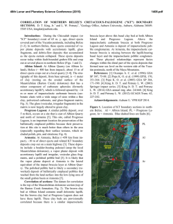


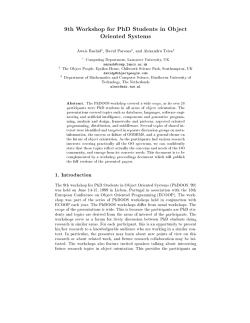
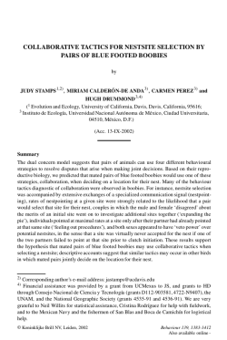
© Copyright 2026