
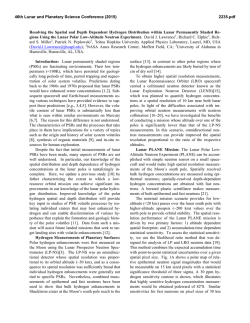
All-reflective interferometric autocorrelator fort
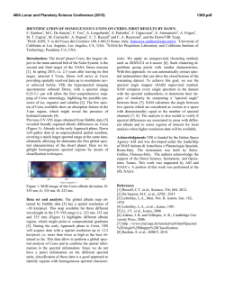
Appl. Phys. B 76, 525–530 (2003)
Applied Physics B
DOI: 10.1007/s00340-003-1148-0
Lasers and Optics
h. mashiko∗
a. suda✉
k. midorikawa
All-reflective interferometric autocorrelator for
the measurement of ultra-short optical pulses
RIKEN, 2-1 Hirosawa, Wako-shi, Saitama 351-0198, Japan
Received: 9 December 2002
Revised version: 18 February 2003
Published online: 5 May 2003 • © Springer-Verlag 2003
ABSTRACT We have developed a novel interferometric autocor-
relator composed of only reflective elements, which functions as
a beam splitter and an optical delay line. Analytical expressions
are derived to give second-order autocorrelation functions and
deconvolution factors for various conditions. The measurement
of femtosecond laser pulses by interferometric autocorrelation
is demonstrated in the visible region. The results are compared
with those by calculation.
PACS 42.65.Re; 42.65.Tg
1
Introduction
Recent advances in femtosecond laser technology
make possible the generation of sub-5-fs pulses, which correspond to two optical cycles in the visible region [1, 2]. Further
shortening has been carried out in various spectral regimes [3,
4], and a sub-fs pulse was obtained by high-order harmonic
generation based on intense Ti:sapphire lasers [5, 6]. From the
viewpoint of the bandwidth limitation to ultra-short pulse generation, it is reasonable to shift the center wavelength to the
shorter side. However, in the short-wavelength region below
the vacuum ultraviolet, measurements of the pulse duration
with conventional autocorrelation techniques are difficult, because the optical components used in the autocorrelator cannot provide sufficiently good transmission and/or reflection
performance. In particular, it is hard to make a replica pulse
and to introduce an optical delay between the original and
replica pulses [7]. For example, the conventional beam splitter
used in a Michelson interferometer is unavailable at wavelengths below the vacuum ultraviolet [8], and it must be replaced by reflective elements.
Recently, an all-reflective interferometric autocorrelator has been developed and demonstrated in the visible
✉ Fax: +81-48/462-4682, E-mail: [email protected]
∗ Present address: Department of Physics, Tokai University, 1117 Kitakaname, Hiratsuka, Kanagawa 259-1207, Japan
region [9, 10], in which a pair of split mirrors functions
as a beam splitter and an optical delay line. The incident
beam is split equally into two by the reflective beam splitter made of the split mirrors. One of the beams is temporally
delayed from the other by slight translation of the corresponding split mirror. The two beams focused together by
a focusing mirror are superimposed at the focal point having the same intensity profiles, but the wavefronts tilt in
opposite directions to each other. The spatial distribution
of the synthesized electric field at the focal point changes
depending on the relative phase, i.e. the optical delay between the two pulses introduced by the reflective beam splitter. The second-order autocorrelation signal can be detected
through a two-photon-induced semiconductor photodetector [11], second-harmonic generation in a nonlinear crystal,
and so on. This technique can be applied to the measurement of ultra-short pulses in the short-wavelength region,
coupled with appropriate nonlinear phenomena for secondorder autocorrelation.
In this article we investigate the fundamental characteristics of all-reflective interferometric autocorrelation by calculation and by experiment. The autocorrelation trace and the
deconvolution factor are derived from analytical expressions
and compared with those from experiments demonstrated in
the visible region. In the following, Sect. 2 presents analytical descriptions of the autocorrelation functions of various
temporal and spatial profiles. Section 3 presents the experimental setup and procedure for preparing the autocorrelator
together with results and a discussion of the measurement of
Ti:sapphire laser pulses. Section 4 is the conclusion gained
from this study.
2
Theoretical considerations
2.1
Spatial profile of split beams at the focal point
First of all, we derive the spatial profile of split
beams at the focal point of the focusing optics. When a collimated beam with a Gaussian profile is split equally into two,
and then one of them is focused with a focal length f l , the
526
Applied Physics B – Lasers and Optics
spatial profile of the focused beam is obtained based on Fraunhofer diffraction theory as follows [12]:
∼
U(x 2 , y2 ) =
i
λ fl
exp −
Then, (1) can be solved and written as
∼
U (x 2 , y2 ) =
x 12 + y12
k
+ i (x 1 x 2 + y1 y2 )
ω2
fl
2 x2
× 1 ± i√
1 F1
π ω0
dx 1 d y1
i
=
λ fl
±∞
exp −
x1
ω
y1
ω
+i
±δ/2
∞
exp −
−∞
2
2
+i
(1)
where ω is the spot size of the initial Gaussian beam, λ the
wavelength, k the wave number, and δ the gap between the
two split beams at the beam splitter. fl can be eliminated using
the following equation that is related to the waist size of the
focused beam ω0 under the assumption of tight focusing, i.e.
the beam waist is located at the focal point of the focusing
optics:
ω0 =
ω
λ fl
≈
.
2
2
πω
1 + (πω /λ fl )
profile
2
,
(3)
∼
U (x 2 , y2 ) =
x 2 + y2
1 ω
exp − 2 2 2
2 ω0
ω0
×
4
1+
π
x2
ω0
2
1 F1
x2
1 3
, ,
2 2 ω0
2
2
(4)
and
ϕ(x 2 , y2 ) =
2 x2
π
± arctan √
1 F1
2
π ω0
1 3
x2
, ,
2 2 ω0
2
. (5)
(2)
If the gap at the beam splitter is narrow enough and
a diffracted wave originated from here spreads out at the
focal point, we can neglect ±δ/2 in the integration in (1),
replacing
it √
with zero. Such an assumption is valid when
√
δ < λ fl ≈ πωω0 .
FIGURE 1
1 3
x2
, ,
2 2 ω0
where 1 F1 is the confluent hypergeometric function [13]. The
sign for the imaginary part in the large parentheses denotes
which half-area is integrated in (1). The amplitude and phase,
respectively, are given by
k
x 1 x 2 dx 1
fl
k
y1 y2 d y1 ,
fl
i ω
x 2 + y2
exp − 2 2 2
2 ω0
ω0
Figure 1 illustrates the spatial profiles given by (4) and (5).
The two split beams have the same electric-field profiles at
the focal point, but the wavefronts tilt in opposite directions
to each other. The spatial variation of the phase is no longer
a function of y2 , which simplifies the analysis described later.
When two beams are superimposed on a plane, the synthesized electric field is expressed as
Spatial profiles of electric-field amplitude a before focusing and b at the focal point. c Phase at the focal point. The original beam has a Gaussian
MASHIKO et al.
All-reflective interferometric autocorrelator for the measurement of ultra-short optical pulses
∞
∼
∼
E (x, y, t) = f(t) U1 (x, y) eiϕ1 (x,y)
−∞
∼
(6)
where the first term on the right-hand side denotes one of
the beams and the second term is the other beam with a time
delay τ . f(t) is the temporal profile of the pulse envelope
and Ω the angular frequency of the pulse. The spatial distribution of the synthesized electric field at the focal point
changes depending on the relative phase ϕ (= Ωτ), i.e. a slight
optical delay between the two pulses. Figure 2 shows examples of the intensity profiles of the synthesized field at
(a) ϕ = 0, (b) ϕ = π/2, and (c) ϕ = π . The second-order
autocorrelation signal can be obtained by integrating the
square of the intensity over the area as a function of the
delay.
2.2
∞
−∞
∞
−∞
dt
−∞
∼
ds E (x, y, t)
4
−∞
∞
∼
ds U (x, y)
∞
−∞
∞
4
−∞
4
∼
4
∼
4
ds U (x, y) sin[2(ϕ1 (x, y) − ϕ2 (x, y))]
∞
∼
4
(9)
−∞
(7)
dt f(t)4 + f(t − τ)4 + 4 f(t)2 f(t − τ)2 ,
∞
dt f(t) f(t − τ)[ f(t)2 + f(t − τ)2] ,
−∞
∞
dt f(t)2 f(t − τ)2 ,
4
ds U (x, y) .
∞
F3 (τ) = 2
∼
∞
−∞
∞
−∞
where the temporal parameters Fi (τ) (i = 1 ∼ 3) and spatial
factors Sj ( j = 1 ∼ 4) are expressed as follows.
F2 (τ) = 4
∼
ds U (x, y) cos[2(ϕ1 (x, y) − ϕ2 (x, y))]
S3 =
S4 =
−∞
+ F3 (τ) { S3 cos(2Ωτ) + S4 sin(2Ωτ)},
−∞
4
ds U (x, y) ,
= F1 (τ) + F2 (τ) { S1 cos(Ωτ) + S2 sin(Ωτ)}
F1 (τ) =
∼
ds U (x, y) ,
The second-order autocorrelation function G 2 (τ) is
G 2 (τ) =
4
ds U (x, y) sin(ϕ1 (x, y) − ϕ2 (x, y))
S2 =
given by
∞
∼
ds U (x, y) ,
Autocorrelation functions
∞
4
ds U (x, y) cos(ϕ1 (x, y) − ϕ2 (x, y))
S1 =
+ f(t − τ) U2 (x, y) eiϕ2 (x,y) eiΩτ ,
∼
527
(8)
The denominators in (7) and (9) are normalization factors for the spatial integrations. The temporal parameters have
been introduced in a number of publications [14]. In the following, we focus on the effect of the spatial profiles, giving
examples of the conventional Michelson-type autocorrelator
and the all-reflective autocorrelator developed in this study.
In the case of a conventional Michelson-type autocorrelator, the problem is quite simple because two beams are superimposed with the same spatial amplitude and phase. Substituting ϕ1 (x, y) = ϕ2 (x, y) in (9), we can obtain a set of spatial
factors ( S1 , S2 , S3 , S4 ) = (1, 0, 1, 0). The second-order autocorrelation function is expressed as
−∞
FIGURE 2
and c ϕ = π
Spatial profiles of a synthesized field for various values of temporal phase corresponding to the delay between two pulses. a ϕ = 0, b ϕ = π/2,
528
Applied Physics B – Lasers and Optics
G MI
2 (τ) = F1 (τ) + F2 (τ) cos(Ωτ) + F3 (τ) cos(2Ωτ).
(10)
If the temporal profile is given by a Gaussian function,
i.e. f(t) = exp(−t 2 ), the temporal parameters are expressed as
follows.
2
F1Gauss (τ) = 1 + 2e−τ ,
3 2
F2Gauss (τ) = 4e− 4 τ ,
F3Gauss (τ) = e−τ .
2
(11)
Then, (5) can be rewritten as
3 2
−τ
+ 4e− 4 τ cos(Ωτ) + e−τ cos(2Ωτ).
G MI
2 (τ) = 1 + 2e
2
2
(12)
In the same way, when the temporal profile is given by
a hyperbolic-secant function, i.e. f(t) = sech(t), the corresponding temporal parameters and the autocorrelation function
are expressed as follows.
F1sech (τ) = 1 +
F2sech (τ) =
sech
F3
(τ) =
6 {τ cosh(τ) − sinh(τ)}
,
sinh3 (τ)
3 {sinh(2τ) − 2τ}
,
sinh3 (τ)
3 {τ cosh(τ) − sinh(τ)}
,
sinh3 (τ)
G MI
2 (τ) = 1 +
Because both S3 and S4 are equal to zero, only the
third term including S1 contributes to the interferometric
properties. Figure 3 shows typical interferometric autocorrelation traces based on (16) and (17), together with the
intensity autocorrelation traces. The interference fringe visibility is 0.54, which is different from the interferometric
autocorrelation traces for the Michelson interferometer. The
lower envelope is only slightly curved on the upper side
and is a maximum at τ = 0. Because of these characteristics it is difficult in practice to find the base line, which
is the same situation for the intensity autocorrelation with
background. Therefore, we define the autocorrelation full
width at half maximum (FWHM) considering just the second and third terms while neglecting the first term, i.e.
unity, in (16) or (17). The deconvolution factor, which is
the ratio of the autocorrelation width (FWHM) to the original pulse width (FWHM), is 1.51 for the Gaussian and
1.66 for the hyperbolic-secant functions. For the intensity
autocorrelation, the corresponding values are 1.41 and 1.54,
respectively. Note that the first-order correlation is a constant, as can be understood from energy conservation in this
configuration.
(13)
6 {τ cosh(τ) − sinh(τ)}
sinh3 (τ)
+
3 {sinh(2τ) − 2τ}
cos(Ωτ)
sinh3 (τ)
+
3 {τ cosh(τ) − sinh(τ)}
cos(2Ωτ).
sinh3 (τ)
(14)
In the all-reflective autocorrelator, the spatial phase is
line-symmetric with regard to the x axis and ϕ2 (x, y) =
−ϕ1(x, y) as shown in Fig. 1c. Substituting ϕ2 (x, y) =
−ϕ1(x, y) into (9), S2 = S4 = 0 because sin(2ϕ1(x, y)) is an
∼
odd function, while cos(2ϕ1(x, y)) and U (x, y) are even
functions. For the others, numerical integration is required
based on (9), and as a result we found that S1 = 0.406 and
S3 = 0. The latter result is probably peculiar to the confluent hypergeometric function, although we were unable to find
an analytical solution. The second-order autocorrelation function is given by
G AR
2 (τ) = F1 (τ) + 0.406F 2 (τ) cos(Ωτ).
FIGURE 3 Calculated interferometric autocorrelation traces for a Gaussian
and b hyperbolic-secant temporal profiles. The bold lines show the intensity
autocorrelation traces
3
Experiment
Figure 4 shows the experimental setup of the autocorrelator. A beam splitter composed of a pair of goldcoated mirrors was prepared by cutting them from a piece of
fused-silica plate after polishing. One of these was fixed on
a mirror holder and the other on a piezo-electric translator
(15)
For Gaussian and hyperbolic-secant temporal profiles,
(15) is converted into (16) and (17), respectively:
3 2
−τ
+ 1.624e− 4 τ cos(Ωτ),
G AR
2 (τ) = 1 + 2e
2
G AR
2 (τ) = 1 +
+
(16)
6 {τ cosh(τ) − sinh(τ)}
sinh3 (τ)
1.218 {sinh(2τ) − 2τ}
cos(Ωτ).
sinh3 (τ)
(17)
FIGURE 4
Experimental setup for the all-reflective autocorrelator
MASHIKO et al.
All-reflective interferometric autocorrelator for the measurement of ultra-short optical pulses
(PI P-841.10) for scanning the optical delay. The closed-loop
control of the piezo-electric translator has a resolution as high
as 1 nm, which corresponds to a temporal resolution of 66 as.
The gap between the mirrors was set to be as small as 100 µm.
The displacement and parallelism of the surface of the mirrors were monitored by a laser displacement sensor (Keyence
LT-8000) while being adjusted using manual actuators (Newport HPS-100) of the mirror mounts. Compared with a conventional Michelson-type autocorrelator, beam splitting and
optical delay are accomplished in a very short distance at the
reflective beam splitter. In addition, the structure is simple and
stiff, which enables the measurements to be both robust and
reliable.
The output beam from a mode-locked Ti:sapphire oscillator operating at 800 nm was used to test the autocorrelator. The pulse width was measured with a conventional
Michelson-type autocorrelator and, as a result, it was found
to be 14 fs FWHM assuming a hyperbolic-secant profile. The
beam was sent to the reflective beam splitter after expanding the beam diameter to approximately 6 mm. Then, the
two beams were focused together by a multilayer-dielectriccoated off-axis parabolic mirror with a focal length of 50 cm.
A GaAsP detector (Hamamatsu G1117) was set at the focal point to observe autocorrelation signals directly from the
two-photon-induced photocurrent. When the first-order autocorrelation signal was monitored, the detector was replaced
by a PIN-Si photodiode.
Figure 5 shows typical signals from the all-reflective autocorrelator: (a) first-order and (b) second-order autocorrelation signals. In Fig. 5a, the first-order correlation signal did
not show any temporal variation, as expected. In Fig. 5b,
the second-order autocorrelation trace gives a FWHM of
23 fs. Based on the deconvolution factor of 1.66 for the
hyperbolic-secant profile, the pulse width is evaluated to be
14 fs FWHM, which agrees well with that measured with the
Michelson-type autocorrelator. It was noted that the fringe
visibility was not as high as in the calculated autocorrelation trace shown in Fig. 3b. This is probably due to the
spatial coherence of the incident beam being slightly degraded by the focusing mirror, the surface figure of which
is not good enough for interferometric autocorrelation. Assuming that only the interferometric term represented by
S1 is influenced, we find that S1 = 0.26 provides almost
the same profile as in Fig. 5b. Figure 6 shows the corresponding autocorrelation trace calculated for S1 = 0.26. However, the deconvolution factor in this case is 1.63, which
529
is different by only 2%. Thus, the measurement is not seriously degraded by such an effect. With a numerical approach, we have investigated the effects of beam profiles
other than a Gaussian, aberration of two beams in a lateral
direction at the focal point, asymmetric beam splitting, and
so on. All results show the reliability as well as the robustness of this scheme, which will be reported in a separate
paper.
FIGURE 6 Calculated interferometric autocorrelation trace, which is the
same as in Fig. 3b except that S1 = 0.26
4
Conclusion
A novel autocorrelator composed of only reflective elements has been developed, which has the advantage
of reducing both the number of reflections and dispersion induced by optical components. Analytical expressions were
derived to give autocorrelation functions together with deconvolution factors. The measurement of ultra-short laser pulses
was demonstrated in the visible region and good agreements
were obtained with calculated results.
If the reflective beam splitter can be made from a spherical or aspherical focusing mirror, the autocorrelation needs
only one reflection. This type of autocorrelator is particularly
effective for optical pulses in the extreme ultraviolet and soft
X-ray spectral regions, eliminating difficulties due to the lack
of good optical elements. It is noted that the intensity autocorrelation is also good for practical use once the setup is verified
with the interferometric autocorrelation.
REFERENCES
FIGURE 5 a First-order and b second-order autocorrelation signals obtained in the experiment
1 A. Baltuska, Z. Wei, M.S. Pshenichnikov, D.A. Wiersma: Opt. Lett. 22,
102 (1997)
2 S. Sartania, Z. Cheng, M. Lenzner, G. Tempea, Ch. Spielmann,
F. Krausz: Opt. Lett. 22, 1562 (1997)
3 A.V. Sokolov, D.R. Walker, D.D. Yavuz, G.Y. Yin, S.E. Harris: Phys.
Rev. Lett. 87, 033402 (2001)
4 N. Zhavoronkov, G. Korn: Phys. Rev. Lett. 88, 203901 (2002)
5 P.M. Paul, E.S. Toma, P. Berger, G. Mullot, F. Aug´e, Ph. Balcou,
H.G. Muller, P. Agostini: Science 292, 1689 (2001)
6 M. Hentschel, R. Klenberger, Ch. Spielmann, G.A. Reider, N. Millosevic, T. Brabec, P. Corkum, U. Heinzmann, M. Drescher, F. Krausz:
Nature 414, 509 (2001)
530
Applied Physics B – Lasers and Optics
7 Autocorrelation measurement of high-order harmonics in the extreme
ultraviolet was demonstrated although a replica pulse was prepared by
splitting the fundamental pulse into two before high-order harmonic generation (Y. Kobayashi, T. Sekikawa, Y. Nabekawa, S. Watanabe: Opt.
Lett. 23, 64 (1998))
8 Use of a transmission grating in an interferometer was proposed in
E. Goulielmakis, G. Nersisyan, N.A. Papadogiannis, D. Charalambidis,
G.D. Tsakiris, K. Witte: Appl. Phys. B 74, 197 (2002)
9 H. Mashiko, A. Suda, K. Midorikawa: In Tech. Dig. CLEO/Pacific Rim
2001 (IEEE, Piscataway 2001) p. II-504
10 E. Constant, E. M´evel, A. Zaïr, V. Bagnoud, F. Salin: J. Phys. IV Fr. 11,
537 (2001)
11 D.T. Reid, M. Padgett, C. McGowan, W.E. Sleat, W. Sibbett: Opt. Lett.
22, 233 (1997)
12 E. Hecht: Optics, 2nd edn. (Addison-Wesley, Massachusetts 1987)
p. 493
13 I.S. Gradshteyn, I.M. Ryzhik: Table of Integrals, Series, and Products,
6th edn. (Academic, San Diego 2000) p. 1012
14 See for example J.-C.M. Diels, J.J. Fontaine, I.C. McMichael, F. Simoni:
Appl. Opt. 24, 1270 (1985)

© Copyright 2026