
PDF version
Hamburg Institute
of International
Economics
It's not all about parents’
education, it also matters
what they do.
Parents' employment and children's
school success in Germany
Christina Boll, Malte Hoffmann
HWWI Research
Paper 162
© Hamburg Institute of International Economics (HWWI) | 2015
ISSN XISSN 1861-504X
Corresponding author:
Dr. Christina Boll
Hamburg Institute of International Economics (HWWI)
Heimhuder Strasse 71 | 20148 Hamburg | Germany
Phone +49 (0)40 34 05 76 - 668 | Fax +49 (0)40 34 05 76 - 776
[email protected]
HWWI Research Paper
Hamburg Institute of International Economics (HWWI)
Heimhuder Strasse 71 | 20148 Hamburg | Germany
Phone +49 (0)40 34 05 76 - 0 | Fax +49 (0)40 34 05 76 - 776
[email protected] | www.hwwi.org
ISSN 1861-504X
Editorial board:
Ph. Dr. Christian Growitsch (Chair)
Prof. Dr. Henning Vöpel
Dr. Christina Boll
© Hamburg Institute of International Economics (HWWI) | January 2015
All rights reserved. No part of this publication may be reproduced, stored in a retrieval
system, or transmitted in any form or by any means (electronic, mechanical, photocopying, recording or otherwise) without the prior written permission of the publisher.
HWWI Research Paper No. 162
It's not all about parents’ education,
it also matters what they do.
Parents' employment and children's school success
in Germany
Christina Boll, Malte Hoffmann
This study is part of a research project partially funded by the Federal Ministry of
Labour and Social Affairs. The full content of the study, any omissions and views
expressed therein are in the sole responsibility of the authors.
© Hamburg Institute of International Economics (HWWI) | 2015
Content
Executive Summary
4
1 | Introduction
5
2 | Theory and hypotheses
7
3 | Data, method and samples
13
4 | Main results
19
5 | Robustness Checks
23
6 | Conclusion
26
References
29
Appendix
A 1 | Endogeneous variables
A 2 | Detailed description of covariates
A 3 | Descriptive statistics of covariates, by samples
A 4 | Sample specification
A 5 | Main regression results
A 6 | Results of robustness checks
35
35
36
40
44
45
49
HWWI Research Paper Nr. 162
3
Executive Summary
In this paper, we use GSOEP data to explore whether parents’ employment has an
extra effect on the school achievement of their children, beyond the well-established
effects of education, income and demography. First, we test whether the source of income or parents’ unemployment determine children’s school achievements. Second,
we analyze the effect of job prestige and factors of societal engagement on children’s
performance. Our results indicate no clear income associations but the existence of an
employment channel as well as a social channel from mothers to their kids. A negative
role model for girls is found for maternal housework. Moreover, the fathers’ job prestige is substantial.
HWWI Research Paper Nr. 162
4
1 | Introduction
Recent literature recognizes that for Germany family background still features not
only success in school but also later income in life (Schnitzlein [2013]). Children whose
parents have low educational attainment less often achieve tertiary education than
children from different backgrounds (OECD [2012]: 107-109). Assuming the distribution of inborn talents being independent from the parental socio-economic status, this
observation implies that potential is wasted. Apart from normative concerns that arise
here, negative long-term consequences for the individual as well as for the economy
are likely to occur (Wößmann/Piopiunik [2009]). The economic view aside, there are
also individual non-monetary benefits of schooling like for instance a larger set of opportunities or better decision making (Oreopoulos/Salvanes [2011]). In order to achieve
the optimal possible school achievement it is important to use every child’s potential.
Child poverty is seen a main cause for suboptimal school achievements (McLoyd
[1998]). Laubstein et al. [2012] identify several factors determining the risk of child
poverty in Germany including parental education, job security, a sufficient income and
the availability of care facilities. This paper contributes to deepening our knowledge of
determinants of school achievement focusing on time use, employment behavior, attitudes and other family background features related to children’s school achievements.
Refining the term family background, parental education is a strong predictor of a
child’s school success. Theoretically, the positive correlation between parental and
child education can have two explanations: One is pure selection, i.e. better parents
choose higher education, the other causal. In obtaining more education one becomes a
better parent. Evidence from the literature is not unequivocal. Björklund and Salvanes
[2010], however, find that parental education plays a minor role in explaining variation
in school achievement. Black et al. [2005] provide evidence that, with one exception,
parental education causally affects the child’s education only to a low degree. The exceptions are mother-son pairs, where increased maternal educational attainment leads
to increased attainment of their sons, too. In contrast, evidence from Plug [2004], who
uses a sample of adoptees, suggests only positive effects from father’s education. Behrman/Rosenzweig [2002], who utilize data on pairs of identical twins, even find a negative, almost significant relationship between maternal education and the outcome.1 To
sum up and in accordance with Teachman [1987], there is evidence that parental education alone does not cover all relevant aspects of family background. The cited findings rather suggest that other attributes, which are more or less closely related to parental education play a role.
1
In adoptee samples, if children are randomly assigned to adoptive parents, genetic factors can be excluded in
the transmission. In twin samples, differences due to genetics can be differenced out between twins.
HWWI Research Paper Nr. 162
5
In this paper, we examine the association of various features relating to family background beyond education in order to shed more light on the driving forces of a child’s
school achievement. The investigated features are deemed to capture parental timeuse, their employment biography and human capital, the household’s pecuniary endowment, and socio-demographic characteristics. Due to data restrictions, the focus of
this analysis is the time where all children are in school, i.e. aged between 7 to 15 years.
To account for sample selection effects we estimate different specifications which are
also checked for robustness amongst others by using two different indicators of
achievement.
First, we test whether the source of income or parents’ unemployment determine
children’s school achievements. Second, we analyze the effect of job prestige and factors of societal engagement on children’s performance. Our results indicate no clear
income associations but the existence of an employment channel as well as a social
channel from mothers to their kids. A negative role model for girls is found for maternal housework. Moreover, the fathers’ job prestige is substantial.
The paper is organized as follows. The next section discusses the theoretical considerations and the derived hypotheses thereof. Section 3 describes the data, the models
and the samples used. Section 4 presents the main results whereas section 5 provides
some additional results from robustness checks. Section 6 concludes.
HWWI Research Paper Nr. 162
6
2 | Theory and hypotheses
In this section, we introduce factors and mechanisms beyond parental education
that, we argue, contribute to explaining a child’s school achievement. We start with the
factors that establish our main six hypotheses and supplement them with core sociodemographic attributes further on. It has to be noted that the importance of many described relationships depends on the child’s age in focus. For instance, the extent of
parental child care is arguably more important for primary school aged children than
for teenagers. As our considered time window is relatively large (9 years), our theory
needs to be somewhat general while the final specification is carried out in the empirical part.
One important factor related to education is parental behavior on the labor market
because it affects several criterions which are considered to be important for the child’s
development and hence its school achievement. Empirical evidence on this topic is
manifold but inconsistent (Goldberg et al. [2008]). This is not surprising given the time, extent- and effect-variant nature of this characteristic. It is, for instance, important at
which age of the child parental employment is measured and how it is measured.
Parental employment can affect the child’s development through at least four interrelated channels, which are: (1) Time spent together with or in the presence of the child
(child care time, housework time, leisure time), (2) the household’s monetary endowment, (3) the transmission of values through role modeling (parenting style), and (4)
the family stress level. The channels and their interactions will be described in more
detail in the following.
Given the daily time restriction of twenty-four hours, parents can spend their time
on labor, child related activities (child care), housework or other activities. The restriction is binding but not necessarily excluding. An increase in working hours, for
instance, does not necessarily imply less time on child care; it might merely shift the
upper bound downwards and time for other activities is reduced. Some kind of tradeoff between child care and employment, however, may be induced. Moreover, this
apparent immediate trade-off can also have long-term effects for the caring parent,
typically the mother. If the time of out-of-labor force (OLF) or the part-time employment is prolonged, future earnings losses will occur, mainly attributable to the depreciation of human capital and/or foregone earnings due to human capital investment
that has not been undertaken during that phase. Boll [2011] calculated expected losses
for diverse scenarios. The induced income losses severely restrict the family’s future
welfare prospects.
Put differently, parental employment can bear positive effects for the child’s development. An increase in working hours will raise a household’s disposable income. In-
HWWI Research Paper Nr. 162
7
come has been found both positively associated (as in Dahl/Lochner [2012] or Duncan
et al. [2011]) and non-significantly associated (as in Løken [2010] or Tamm [2008]) with
the child’s success in school. Several possible transmission channels were suggested in
the literature: Direct effects include enhanced possibilities to purchase inputs favorable
for the school achievement (Becker [1965]), e.g. by affording private tuition, moving to
a better neighborhood, a reduced risk of stigmatization or even less parental stress
(McLoyd [1990]). Schneider [2004] shows for West Germany that a higher maternal
education does not prevent the household from purchasing private tutoring and
homework help.
Akee et al. [2010] argue for an indirect effect: in a quasi-experimental study about the
effect of an increase in household income on parental interactions with their children, a
share of the profits from a newly built casino is periodically distributed to Native
Americans but not to Non-Native Americans. This is an exogenous increase in household income for the first group. The authors compare the groups and find that individuals in this group do not reduce working time due to the windfall. The positive effect
on school achievement the authors found is mainly attributable to improved parental
interactions and experiences with their children. Their measures are the parents’
statement on how often they know the whereabouts of their child and the child’s
statement on how much of the time spent together with their parents they consider to
be enjoyable. The authors also emphasize that a larger effect occurs for low-income
families. Others pointed out that low household income can increase the risk of separation and divorce (D’Addio [2007: 31f]). The latter occurrences are negatively related to
the child’s school achievement (Björklund/Sundström [2006]).
Based on the cited literature, we hypothesize that, in general, a higher household income is associated to better school achievements of children. However, the question
arises whether the effects differ between different kinds of household income, i. e. maternal and paternal labor income. Results for the latter could indicate the existence of
labor division and specialization effects or effects of role models and values conveyed
with maternal and paternal employment. Relatedly, the propensity to work is negatively influenced by income types such as asset income or public or private transfers
since they are non-labor income (Borjas [2010]). For employment can carry more than
monetary benefits and underlying parental characteristics will not be fully ascertainable, we suggest that the source of income matters: income stemming from public transfers will be different from income from labor. We therefore hypothesize:
Hypothesis 1
We expect different effects of different sources of income. In particular, the receipt of public
transfers is expected to be negatively associated, while income stemming from labor will be positively associated with the child’s outcome.
HWWI Research Paper Nr. 162
8
With regard to the effect of parental unemployment there is evidence for a negative
association between paternal job loss and school achievements (Gregg [2012]). Bratberg
et al. [2008] on the other hand find no long term effect on children’s earnings for Norwegian data. Rege et al. [2011] find a negative effect on school performance only for a
father’s job loss, but the effect could not be confirmed for maternal job losses. This is
elucidated by the observation that mothers often extend child care time after losing
their job, while for men the break with the traditional breadwinner model leads to psychological problems in the family. Despite having the same number of nominal working hours, namely zero, this implies a need to differentiate between (involuntary) unemployment and (voluntary) OLF time. Apart from the scars that arise through the layoff, it leads to the opposite effects of the previously described benefits of employment
and is also associated with arising psychological problems and low self-esteem (Ström
[2003], Sheeran et al. [1995]). Low self-esteem, in particular, is considered to change
parental expectations for their children to the negative (Kaplan et al. [2001]). We therefore hypothesize:
Hypothesis 2
In relation to the other statuses, parental unemployment is negatively affecting achievement.
A fundamental issue underlying all effects arising through employment is its extent.
Depending on the working hours and conditions, employment might affect the family
stress level and thus the environment where a child grows up. An effect can be positive
if sorrows due to low income and social stigmatization are mitigated by higher income.
Negative effects are also conceivable if, for instance, the job requires frequent unexpected overtime or leaves too little time for remaining activities. This time trade-off
holds particularly true for the more highly educated who work more overtime hours
than others [Zapf 2012]. Moreover, it applies especially to mothers who are traditionally more in charge with the care of their offspring than fathers. Findings of Felfe and
Hsin [2012] show that maternal work-related hazards and stress negatively affect the
child’s development. Their results also portend that compensating maternal time investments are indeed significant but have a small effect.2 Because overtime is positively
related to the number of working hours (Institut der deutschen Wirtschaft [2014], Zapf
[2012]) we hypothesize not only that high working hours tighten up parental time
budgets but are also linked to the stress level within the family and that this particular-
2
The linkage between mothers’ time devoted to their children and the offspring’s outcomes later in life depends also on the quality. The findings of Datcher-Loury [1988] show that extended time use on child care of
highly educated, but not of less educated mothers, significantly increases children's years of schooling. Recent evidence from Kalil et al. [2012] demonstrates that more educated mothers spend more time on childrelated activities that promote the child’s development than less educated mothers do. Thus the amount and
the quality of parental care time must both be regarded; often, however, only quantitative information is accessible as in the case for the used SOEP data.
HWWI Research Paper Nr. 162
9
ly applies to mothers.3 Whether the relationship is linear or not is not clear a priori. We
therefore hypothesize:
Hypothesis 3
We expect negative effects by high working hours, particularly of mothers.
A fourth channel arises when the idea of a parental role model is applied. Employment can signal the child commitment, social participation and in the case of maternal
employment also a modern view of a woman’s role in society (Röhr-Sendlmeier [2009;
2011]). Often, the role model is interpreted as an intergenerational transmitter of attitudes. Fernandez, Fogli, and Olivetti [2004] and Morrill & Morrill [2013] find that
women are more likely to participate in the labor force if their mother had already
worked. This correlation also remains stable between mother-in-law/daughter-in-law
pairs. With regards to other positive effects, Alessandri [1992] found that children with
employed single-parent mothers have greater self-esteem than children with nonemployed mothers and girls whose mothers are full-time employed had higher academic achievement. Finally, Anger [2012] notes that the older children get the more
similar their personality becomes to the parental one. In terms of maternal autonomy
and employment, this might have a positive influence on a child’s, in particular a girl’s,
achievement. We therefore hypothesize:
Hypothesis 4
Maternal employment, for girls in particular, is positively associated with the outcome
through role modeling.
One characteristic that has not been paid attention to yet is occupational prestige. In
spite of its high correlation with income and education, it can be argued that parental
social status relates not only to income but also to occupation. Furthermore, occupational prestige might reflect parental aspirations concerning human capital formation.
We therefore hypothesize:
Hypothesis 5
Beyond education and income, parents’ occupational prestige impacts positively on the
child’s schooling outcome.
To improve the view on the family life, additional ‘soft factors’ should be regarded.
Extending our argumentation that occupational prestige and education carry aspirations, which we assume to correlate with the aspirations parents hold for their children, there is evidence that such aspirations are substantially heterogeneous across
3
The study shows that almost 80% of full-time employed workers, but only 65% of the part-time employed,
work long hours. The data are from 2011.
HWWI Research Paper Nr. 162
10
similar levels of formal education (Ehmke [2009]; Paulus/Blossfeld [2007]). As the
measurement of aspirations is typically rather complicated or subject to data limitations, we use a different approach. It attempts to shed more light on family life and
parental aspirations by regarding indicators of parental interests and activities. Certain
characteristics relate to personal aspirations and also to milieus in which certain norms
for activities, attitudes and aspirations are hold up. Because the question of whether
the milieu shapes personal characteristics or the milieu is chosen according to personal
preferences is difficult to answer, we simply refer to the observed characteristics and
argue through an indirect channel. We thus construe aspirations from family life, expressed by personal interests and behavior. We hypothesize:
Hypothesis 6
Given parental education, income, and employment features, parents’ leisure activities and
interests relating to parental a#itudes and aspirations will still have an effect on the child’s
school outcome.
Suggested influence from socio-demographics on the child’s outcome
Beyond parents’ human capital and employment, socio-demographic attributes are
found to have a bearing on the child’s development. We will therefore control for a
range of demographic factors. For instance, the existence of a partner and his or her
time use play a key role. In general, couples face a lower risk of low household income,
specialization in household duties can take place and events like unexpected unemployment can be cushioned better. Also the compatibility of family and career is harder
to attain for lone parents since they would, for instance, ceteris paribus need more time
for work to sustain a certain level of income.
Another aspect concerns the child itself. With respect to school performance, girls
achieve better grades on average than boys (Voyer/Voyer [2014]). Furthermore, from
an intra-family resources view, the number of siblings in relation with the birth order
may also play a role (Lindahl [2008]; Booth/Kee [2005]). While many siblings decrease
the parental resources left per child, being the first-born has the advantage that the
previous effect will eventuate later. On the other side, parents gain experience from
raising kids which can affect the later-born positively. A more general experiencerelated argument is the parents’ age. As Nechyba et al. [1999], based on evidence by
Geronimus et al. [1992], point out, this correlation is likely to be non-causal as underlying characteristics influence both the time of birth and the child’s development. Particularly, birth timing is associated to the mother’s education. In Germany, for instance, a
positive correlation between education and age of first birth is observable (Boll et al.
[2013]). Highly educated mothers face higher opportunity costs of child bearing and
rearing, whereas the care time investment for each child is assumed not to be lower
than a certain threshold [Oreopoulos/Salvanes 2011]. Moreover, according to Becker’s
HWWI Research Paper Nr. 162
11
quantity-quality model, the demand for child quality increases with parents’ education, resulting in fewer children (Becker/Lewis [1973]). We expect that preferences for a
high child quality particularly address the first born child and motivate a rather low
number of siblings in general. Hence, they should benefit the educational performance
of the first born more than that of his or her junior siblings provided they exist. Finally,
the number of siblings is related to the mother’s age at first birth since productiontechnological restrictions might stipulate births at the end of the fertile life span of
women. All in all, maternal age, education and the number of siblings are likely to be
interrelated but their effect on the outcome variable is a-priori ambiguous. Hence, we
control for each factor separately.
Considering the relationship between parental separation and divorce, a negative association can be ascertained. The main reason is distress for the child. It has been
found, however, that the distress fades over time for the majority. The minority for
which this does not apply achieves particularly bad outcomes on the other hand
(Rodgers/Pryor [1998]). A different view on the topic is due to Björklund and
Sundström [2006]. Using a sibling-difference approach, their findings suggest that the
negative association between separation and children’s development is rather due to
selection than to causality. That is, unobserved parental traits that negatively impact
children’s school achievement also enforce separation. As we control for many factors
that might capture to a certain extent parental unobservables related to their propensity of separation, we do not expect to find a significant effect from separation or divorce
by its own, pointing to a causal effect.4
4
Another important factor is the peer group that can have an important influence, in particular in teenage
years. However, our dataset is limited regarding suitable data on this topic (Lohmann et al. 2009) - only milieu indicators might capture some of the effect. Hence, we do not explicitly consider this issue here.
HWWI Research Paper Nr. 162
12
3 | Data, method and samples
We make use of the German Socio Economic Panel Study (GSOEP, v29, see Wagner
et al. 2007), where we link parental data to child’s data from the youth questionnaire of
the years 2000-2012. As the outcome is available for only one point in time, our analysis
is a cross-section analysis. Owing to the restrictions in the number of observations, we
consider retrospective parental data only from the time onwards when the child was
enrolled in school.
Dependent Variables
To check the robustness of our results we use two different endogenous variables.
One is the (expected) school leave degree (ESLD), the other is a Grade Point Average
(henceforth: GPA). Their advantages and disadvantages are inversely related. Using
the expected school leave degree discards variation within a certain school type since it
does not regard the variation in grades; it accepts, however, the structure of the educational system. 5 By contrast, the calculation of the GPA requires a scheme to convert
grades between school types. Such a scheme does not exist in general. On the other
hand, grade variation within a school type is regarded. The dependent variables are
measured at about the age of 15 to 17 which is close to or already the end of a school
career. The first variable carries the interpretation that only the type of graduation matters in later life as – except for those who resume a higher schooling degree later in life
– it paves the way for the highest feasible educational level and henceforth career perspectives.6 The second variable regards the heterogeneity in individual performance
somewhat more and might therefore be more informative.
We base ESLD on either a finished school graduation or, if the child is still in school,
on the usual graduation for the current school it is on. The latter typically only applies
to pupils on the Gymnasium – pupils on other school types are graduated from before
the age of 17 if no grade retention or comparable events took place. The ordering follows the level of requirement. If possible, we double-check the school graduation with
5
6
There are three main secondary school types in Germany. They differ in requirements to attain a certain grade.
The highest standards are found at the upper secondary school (”Gymnasium”), the lowest at the lower secondary school (”Hauptschule”). In between is the middle secondary school (”Realschule”). The grades on
each school range from 1 (the best grade) to 6 (the worst grade). The different requirements and outcomes
can be used for evaluation of school achievement. There are, however, more but less often visited school
types in Germany – a fact that is also reflected in the GSOEP. For the purpose of this paper, it is convenient to
assign these to the scheme above. Therefore pupils at technical secondary schools were assigned to the
Gymnasium. Pupils currently at an occupational school were assigned to the type of school they were visiting
before. This is done because there is a plethora of different occupational schools in Germany which also cannot be sensibly ordered. The assumption is that pupils would self-select into further education that meets
their standards, neither higher nor lower.
Although in principal, a lower secondary school degree does not make tertiary education impossible, de facto
only few persons graduating from lower secondary school enter college later in life (Statistisches Bundesamt
[2013]).
HWWI Research Paper Nr. 162
13
GSOEP-data obtained from later questionnaires. This procedure also allows including
pupils from comprehensive schools where the type of graduation can be unclear. Differences in the graduation rates between the German states imply that the requirements to be on a certain school type vary or, put differently, the distances between the
threshold values for the underlying latent continuous variable are specific to each
German state. In order to remove such differences, we standardize the measure on
state level, so the variable becomes metric.
The GPA is computed from answers to the questions about the last grades in the
main subjects German, Mathematics and the first foreign language. The answers were
given once for all by the adolescent when he or she turned 17. Some individuals reported finer information in terms of half point grading which is incorporated. To obtain a single variable that can be compared across pupils from different school types,
differences due to valuation standards have to be removed and the grades from three
subjects have to be merged. The transformation between school types is based on the
“Hamburger Stadtteilschule” transformation scheme. Hereby, a new scale, ranging
from 1 to 9 is created. The grades from pupils on the upper track secondary school are
transferred one-to-one on the new scale. The grades from pupils on the other schools
are transformed. If a pupil achieved the best grade, i.e. a 1, in a subject at the school
type with the lowest requirements (Hauptschule) the “transformed” grade at the most
difficult school (Gymnasium) is a 4. The grade on the new scale is then accordingly 4. If
the pupil on lower secondary track did not achieve a 1 but the second worst grade, that
is a 5, the corresponding grade on the new scale will be 8. Pupils at comprehensive
schools have subject-specific valuation standards. Thus, they are subject-wise assigned
to the three basic school types Hauptschule, Realschule and Gymnasium. For convenience of interpretation in the regressions, the new scale, which ranges from 1 to 9, is
reversed such that favorable grades are larger than unfavorable ones. Table 2 in Appendix A1 provides an illustrative example.
Extending the previous measure of success, we standardize the grades for each subject statewise. In so doing, we account for both general and subject specific differences
in level and variance between federal states. To have a large enough number of observations when standardizing, all grades over the years acquired in a certain federal state
were pooled. It is hereby assumed that the relative requirements in each federal state
remained stable over the decade.7 The final step is to apply the arithmetic mean to the
standardized grades on the three subjects.
In creating the dependent variables with the described method, we transformed two
variables initially containing ordered categories to two more or less metric ones. While
the GPA appears metric, the (expected) school leave degree kept some of its categorical
7
Saarland and Rhineland-Palatinate were treated as one federal state for data reasons.
HWWI Research Paper Nr. 162
14
character (please find the respective histograms for the two dependent variables in
diagram 2 in appendix A1). Yet it consists of sufficiently many distinct observations.
For both dependent variables, we therefore apply ordinary least squares.8
Explanatory variables
According to the goal of this paper to evaluate the additional effect of parents’ employment on their offspring’s school achievement, we partition the set of explanatory
variables into three groups which are successively added in the estimation process (diagram 1). The first set includes socio-demographic variables only (model I). Model I is
enriched by human capital related variables of income and education yielding model
II, and model III additionally comprises variables related to parents’ employment status and employment biography.
Table 1
Model types
Model I
Model II
Model III
Socio-demographic variables
Socio-demographic variables
Socio-demographic variables
Human capital variables
Human capital variables
Employment status, employment
biography
With our list of covariates we extend former analyses in two aspects, (a) our income
variables are more fine-grained in order to investigate the particular importance of
labor earnings, and (b) we furthermore add an indexing variable of ‘soft factors’ to the
demographic variables that has been exclusively constructed for this analysis. However, the third category that comprises of the employment biography variables represents
the focus of this paper.
Appendix A2 provides a comprehensive variable description and Table 4-7 in appendix A3 the respective summary statistics, so we will not go into details here. In
short, as to the socio-demographic variables, we control for the state of living together
with both parents or one parent only, the number of siblings, birth order, parental age,
milieu, migration background, daily workloads concerning household and childcare
tasks, and the family’s number of moves. Human capital related variables comprise
years of attained education of each parent and four income categories (net household
income, gross labor earnings, asset income, private and public transfers). Employment
status and biography related variables refer to the factual weekly working hours (of
8
We abstain from using robust standard errors as the differences to ordinary standard errors turned out to be
small.
HWWI Research Paper Nr. 162
15
mothers in the child’s age span 7 to 9 only) and the years of full-time employment,
part-time employment, years out of the labor force (OLF), years of further education
and years of unemployment (the latter serving as a reference category) of each parent.
Finally, this category is completed by information referring to the occupational prestige
given that the parent is (or has at least once been) employed.
Samples
If one attempts to explain school achievement, the relevant characteristics of all
available parent (-like) household members should be regarded. In not so few cases,
however, the household composition changes, household members leave the household or are perhaps replaced by other persons. Owing to potential time variation within the scope of nine years, including partner data would require strong assumptions on
a model and also not be feasible for some households at all. We therefore estimate two
different sample specifications which address this issue.
In the first specification, a child’s data is linked separately to only the mother’s and
only the father’s characteristics, respectively, not directly regarding possibly available
partner data.
The link is established by the information about the respective parent’s personal
number in the youth questionnaire. If we merge the child’s data with parental data via
the mother’s personal number, the mother is termed as reference parent. The data that
has been linked to the child will refer solely to the mother. If we merge via the father’s
personal number, the father is called reference parent. The data that has been linked to
the child will refer solely to the father, then.
In addition to the implicit restriction that the parent must exist (in the GSOEP), one
more restriction is set up, however: In the data set where child’s data are linked to the
mothers’ data, the mother has to be in the GSOEP at all considered times, i.e. from the
child’s age of 7 to 15. The same has to hold true for the father for the data set where
child’s data are linked to fathers’ data.9 This first specification leaves us with two samples – one with the mother as the reference parent, one with the father in this position.10
Note that the fact that the parent has to be in the SOEP at all considered times is likely to threaten sample
representativeness. Evidence is provided by Spieß / Kroh [2008] who predicted the probability of reinterviewing versus refusal in the year 2006. Amongst others, non-German households and households experiencing separation and unemployment were associated with an increased risk of attrition. As argued, these
factors are also related to the child’s school achievement. Hence, even the sample disregarding partner information might be positively selected with regards to the endogenous variable.
10 One might criticize that some children grow up with only one parent, say the mother, but supply both parents’
personal numbers. Linking the child with father’s data in this case might then be somewhat misleading. But
although the child lives officially with the mother, we cannot exclude that the child spends much time with its
father. Hence, we use the data if available, although the influence is most certainly heterogeneous across the
children.
9
HWWI Research Paper Nr. 162
16
Although it is sometimes possible to merge parental partner data to the data set in a
second step, there is an advantage not to do it. If data of only one parent is used, the
household composition is allowed to change, for example due to a separation of parents. However, the partner data are of interest, too, therefore a second specification is
set up.
The second specification embarks with linking the child’s data again to either the
mother or the father and activating the restriction on the parent to have participated in
the GSOEP in the considered time range once more. Then each sample is further restricted to those who lived together in a relationship with one and the same person
during the whole period from the child’s age 7 to 15. The person is called partner and
also has to be in the GSOEP in the considered period. Given the constant partner, we
can enrich the model with partner data. We treat cohabitation, marriage and switching
between the two states as the same. The important aspect is to have one and the same
partner during the whole period. Those who were at least once in this period without a
partner or switched the partner are hence excluded. The two partner data samples with
one time the mother being the reference parent, the other time the father, have many
observations in common (just in “opposite positions”) but they are not completely the
same: if, for instance, both biological parents live separated and one or both have new
partners, who are also in the GSOEP, the information differs.
Note that the time horizon of the aforementioned “living” variables is different from
that of the constant partner: Having lived together with mother and father or one parent only focuses on the child’s age span 0 to 15. Moreover, the living variables also address the issue of biological parents whereas the constant partner restriction does not.
This second sample specification leaves us with two more samples – one with the
mother as the reference parent and one with the father in this position. Note that due to
the additional restriction of stable couples, the two samples of specification 2 are subsamples of the two samples of specification 1.11
The restriction of stable couples is likely to cause positive selection effects with respect to the outcome variable as stable partnerships are expected to positively impact
on the child’s development. As stable partners have to be observed, there is a double
selection. We therefore check the effects of partnership survival on the main endogenous variable, the expected school leave degree. We perform t-tests on the equality of
the mean value. We do not find significant mean-value differences for samples without
11
One critique by Björklund/Chadwick [2003] points at caveats by treating biological and non-biological fathers
the same: regarding intergenerational income mobility, the association between the biological father and the
child is much stronger, presumably due to inherited ability. This indicates potential differences also for other
outcomes. We ignore the issue for two reasons: Firstly, we restrict the sample to partners that were there at
all considered times, the difference might therefore not be expected too strong. Secondly, the low number of
cases would make separate analyses difficult. Please find detailed information on the descriptive comparison
of endogenous variables in Table 3 of A2 in the appendix.
HWWI Research Paper Nr. 162
17
partner data. For the expected school leave degree in the mother’s sample with partner,
we run a one-sided t-test (with unequal variances). The test results indicate differences
in the mean value at the 10%-level. The same t-test result applies to father’s samples
with partner. Moreover, the average expected school leave degree is somewhat higher
in our stable partnership-samples than on average.12 That is, indeed, the results hint at
a slightly positive selection of stable couples that requires to carefully interpret results
arising from sample comparisons. However, as we are more interested in the structural
information within samples this finding does not cause us to modify our specification
strategy.
Through incorporating the maximum value of the prestige variable during the considered period, individuals who have never worked in that period are dropped from
the sample. In order to take into account potential selection effects due to the employment restriction, we have estimated several specifications. For the analyses without
incorporated partner data, each model was estimated with the full sample, but also
with the sample for which the restriction “at least once employed during the regarded
period” binds (for a visualization, see Table 7 in appendix A4)
We chose the sample with binding restrictions for both parents as the main samples.
Therefore, in Section 4 only results referring to this specification are discussed. Important
deviating results from other specifications are reported in Section 5.13
For the analysis with considered partner data, each model was additionally estimated under the restrictions “partner at least once employed during the regarded period”
and “reference parent and partner were both at least once employed during the regarded period”. One exception occurred in the father’s samples: if the female partner
was employed, then the father was, too. So the restriction “reference parent and partner were both at least once employed during the regarded period” is equal to “partner
at least once employed during the regarded period” in this case. Again, we selected the
samples with binding restrictions for both parents as the main samples.14 See the appendix for a descriptive table. Tables 9-12 in appendix A5 show the results for our selected specifications.
Please find detailed information on the descriptive comparison of endogenous variables in Table 3 of A2 in
the appendix.
13 Detailed results from the full sample may be provided on request.
14 We could find some slight changes when the restriction held for the female part. The effect through the paternal restriction affected only a small number of observations and virtually no differences were visible, thus
these results are not shown at all. This observation also implies that most men were at least once in employment.
12
HWWI Research Paper Nr. 162
18
4 | Main results
Generally, it is notable that the results for the samples with partner data are often
similar. The reason is that in many cases the same parental individuals are present, just
in opposite positions. But as described in section 3, the samples are not the same. One
observation concerns the sample selection of parents which reduces the variation in
some of the variables. In particular, the stable households are marked by little variation
in paternal employment and few cases unequal to zero in some of the “number of years
living together with”-variables. So there is some stability in family life which suggests
that the sample mainly consists of rather unproblematic, homogenous households.
Indeed, children in stable partnerships face somewhat more favorable outcomes. However, as we will show in more detail below, the structural information gained from
those samples resembles to a wide extent the patterns observed in samples without
considered partner data.
For the socio-demographic variables we find results in accordance with the literature.
Robust effects are ascertained through the child’s gender whereat we find girls attaining
higher achievement than boys. The effect is typically of the magnitude of about a third
of a full grade. The position in the birth order turns out to be of noticeable importance,
too, with the more advantaged the sooner born. The number of siblings is sometimes in
the first model significantly positively, but never negatively, associated with the outcome.15 The number of moves in the last nine years, although mostly negatively related to
the outcome, plays no significant role.
The dummy variable for living in former East Germany is exclusively positively significant and also exhibiting quite a strong effect. This is surprising as the dependent
variable has undergone state-level standardization. Analyses divided according to the
child’s gender reveal that the effect is driven by sons. The indicator variable for living
in a rural area is in most models significantly negatively associated with the outcome.
However, the effect is slightly diminished once human capital and employment biography of parents are controlled for and even becomes insignificant in the samples with
partner data.
Furthermore, in the mother samples and also in some of the father samples, there is a
negative association of maternal housework in the period where the child was aged between 7 and 9. We provide two explanations. One is that the variable might take up
some negative effects through unemployment as women might tag their “free time” as
housework to avoid stigmatization. The other one is linked to the role model channel: a
mother doing a lot of housework embodies the traditional role model and daughters
15
It is possible that birth order already takes up some of the siblings’ variable’s effect, because a high birth
order is only possible with several siblings.
HWWI Research Paper Nr. 162
19
will not enjoy potential benefits of a working mother. This interpretation is strengthened by additional analyses presented in Section 5 which indeed show that the negative effect is driven by the daughters in the sample: boys are not significantly affected.
As expected, parental age is positively associated; the effect is diminished if variablericher specifications are chosen, but remains highly significant. The weakening of the
effect when human capital variables are controlled for is in line with expectations since
a positive correlation between the parental age and income or education can be expected.
One interesting result concerns the soft factor variables: paternal soft factors are a lot
less significant than maternal soft factors once maternal soft factors, paternal years of
education and paternal income are controlled for. Paternal soft factors even become
insignificant in some specifications. This is remarkable, since they are highly significant
in father samples without partner data. Analyses split by the child’s gender indicate
that the stronger maternal effect is driven slightly more by the sons in the sample (see
Section 5). We further observe that a soft variables’ effect size dwindles by roughly a
half when the set of human capital variables is added – the main reason being its correlation to education.
Moreover, no effects are brought about by parents having direct migration background. Indirect migration background exhibits negative associations in the first model
of the father’s samples; the results are not robust, however.
We now discuss results for human capital variables. Our results for parental education
are as expected: a highly significant, positive association to the child’s expected school
leave degree can be found. In contrast to former analyses in the literature, remaining
effects through inherited abilities and assortative mating are not excluded in our analyses.
With regards to income variables we found mixed results. First of all, asset income is
only weakly significant or insignificant in father samples with partner, otherwise not
significant. We hence dropped the variable from our estimations. Starting by discussing labor income, we find that in samples with the mother being the reference partner
and excluded partner information, it is negatively associated with the child’s outcome.
It is unlikely that money harms the outcome, instead, underlying characteristics like
many working hours are more likely to explain the negative association. Also a slight
correction effect to the positive coefficient of net household income can be adduced as
an explanation. In samples with partner data, the corresponding variable is insignificant. The effect of the father’s labor income is overall not significantly different from
zero. We suggest a possible reason for that, which is a noticeable correlation between
household income and paternal labor earnings. This explanation might also be applicable to samples with stable partnerships. When it comes to public transfers, we find
HWWI Research Paper Nr. 162
20
negative associations for the samples without partner data for model II and one positive effect for public transfer income in model III for the mother sample with partner
data.
Net household income turns out to be highly positively related to the outcome variables in most mother samples, in particular for samples without partner. A high
household income might not only indicate sufficient monetary endowment but in those
samples also hint at a stable relationship because the partner contributes to the household income. Private transfers play solely a role in the second model of mother samples
without a partner. In sum it can be observed that many effects shrink when the model
is enriched with variables of the employment biography.
As to employment variables, we find negative effects for the factual number of maternal
working hours between the child’s age 7 and 9, the variable is significant in merely one
specification, however. In further analyses, we examined the influence of overtime in
several specifications which were mostly insignificant. Furthermore, the overtime coefficient would be difficult to interpret due to reduced number of observations that result
from the construction of the variable. It requires information on contract working
hours that lacks for amongst others the self-employed. We therefore skipped the overtime variable. We also tested the hypothesis of a quadratic increase in effect of factual
working hours, but this could neither be confirmed and was also skipped.
While maternal maximum prestige is only significant in the samples without partner
data, paternal maximum prestige exerts an overall highly significant positive effect,
also when maternal maximum prestige is simultaneously included. The effect size for
paternal maximum prestige also exceeds the maternal one by far when the samples
without partner data are compared. Sub analyses show that the effect of education is
diminished once the prestige variable’s is included. Using the average prestige value
over the years of employment instead of the maximum value does not change any of
these relations substantially.
With regards to the employment biography, we find much stronger effects for the
mother or the maternal partner than for the father. This is attributable to little variation
in the respective information for fathers.16 However, we observe that weak positive
effects emerge from years in full-time or part-time in samples without partner. In the
double-selected, more homogenous samples with partner, no significance can be established. It makes therefore more sense to only scrutinize the maternal employment variables in more detail.
16
Fathers’ mean years in full-time employment are about 8 of 9, while the mean months spent in unemployment are roughly 6 and part-time and OLF experience as well as educational training are even less present.
This also likely explains why we find no effects for factual paternal working hours.
HWWI Research Paper Nr. 162
21
Recall that unemployment is defined as the reference group. The category “further
education” is generally suffering from low variation which makes the coefficients unstable and therefore the variable is not sensibly interpretable.
One can observe highly significant positive effects for maternal full-time and parttime employment as well as years OLF. This holds true for mother samples without
and with partner and also for father samples with partner. The effect size of full-time
and part-time employment is typically at least as strong as that of OLF. In mother
samples with partner and the more so in father samples with the mother as the partner,
effects are less significant and OLF time loses significance in the latter sample. Thus
there is clear evidence that maternal labor market participation is positively related to
the child’s outcome. It is hereby unclear whether full-time or part-time employment is
more beneficial. The effect size differs across samples.
HWWI Research Paper Nr. 162
22
5 | Robustness Checks
This section demonstrates that some of the results are sensitive to the choice of the
dependent variable, the gender of the child, to sample restrictions and the specification
of core covariates.17
We begin with comparisons between the two endogenous variables, the results are
provided in Table 16 and 17 in appendix A5. For overview reasons we focus on presenting noticeable different results for model III only. In comparing the samples for the
different endogenous variables, we note that some differences are stable across the
samples with and without partner data. The gender effect is stronger or more significant for the GPA, while the influence of living in the new “Länder” is in absolute terms
smaller for the GPA than for the expected school leave degree.
Independent of whether the mother is the reference parent or not, the daily amount
of maternal housework between the child’s age 7 to 9 is more robustly negatively associated with the expected school leave degree. The same holds true for the maternal
employment biography variables in samples without partner data.
Results furthermore differ by the child’s gender, as gender-divided samples show (see
Table 20 and 21 in appendix A5). The following results are striking: The positive effect
of living in the new “Länder” is driven by boys in the sample. Another interesting
gender-specific aspect concerns the effect of the soft-factor index variable: It is observed that sons are almost exclusively influenced by the mother’s soft factors while
the girls are also, but only slightly, influenced by the father’s soft factors variable.
The negative effect of maternal housework is, as described before, affecting girls
much more than boys. We refer to the role model explanation here. Mother’s employment biography (full-time, part-time or OLF with unemployment as reference time)
matters more to daughters than to sons in samples without partner data. This applies
in parts also to maternal occupational prestige and holds for all samples with the
mother being the reference partner irrespective of considered partner data. Note that
employment is correlated with labor income, the latter partly exhibiting gendered effects on children’s school outcomes. In mother chaired samples without partner, maternal labor income is negatively associated to daughters’ outcomes but lacks significance for sons. Apparently, the positive gender role model does not operate via the
earnings channel but via the parent’s time investment decision itself. This particularly
holds true for mothers. However, intense labor market involvement of mothers produces contrary effects, the same applies to intense housework. It seems that a moderate
attachment of mothers to the market suits their offspring’s outcomes best. Furthermore
17
In the appendix, only a shortlist of results is presented. Full results of all robustness checks may be provided
on request.
HWWI Research Paper Nr. 162
23
some cross-gender effects may be portrayed. Boys are positively affected not only by
their mothers’ soft factors but also by their labor market success (particularly in mother
samples without partner) and maternal prestige (particularly in stable partnerships
chaired by the mother). Paternal employment biography lacks significance for boys
and girls but this is presumably due to low variation in the data as most fathers are
continuously full-time employed.
Sample restrictions in this paper refer to the employment restriction (parent being at
least once employed in the time span 7 to 15) and to the stable partnership restriction.
The effects of the latter have been well documented above, so robustness checks address the employment restriction solely. It turns out that the restriction is almost exclusively binding for mothers, as almost all fathers or male partners were once employed.
Being at least once employed in the considered period is a precondition for measuring
occupational prestige. One robustness check compares the results for the third specification under different maternal employment restrictions, see Table 18 and 19 in appendix A5. We only compare results for the mother as reference parent. In the samples
without partner data, we find only slight changes, our results seem to be robust. When
partner data is included, the results mainly change with respect to the effect size. In
particular, the employment biography variables get more influential once the maternal
employment restriction is activated.
We further run two calculations with modified specifications of covariates, 1) our income variables, 2) occupational prestige, 3) an added tracking recommendation variable and 4) milieu factors included.
1) As mentioned in Section 3, we also run a specification that differentiates between
income accrued in the child’s age 7 to 9 and 13 to 15, respectively as a robustness check
of our main specification of pooled income information from 7 to 15. The results
essentially resemble those of our main specification. This particularly applies to the
positive association of net household income and the negative association of public
transfers, both findings being mostly reserved to samples with the mother being
the reference parent. A noteworthy exception refers to maternal and paternal labor
income that are insignificant throughout all estimations, maybe due to an inherent
path dependence of labor market returns.
2) We also calculated mean occupational prestige for available years. Since occupational
prestige is usually slow to change, this did not change the results in any substantial
way.
3) We further checked a specification that includes a tracking recommendation variable
as an additional regressor (enlarged model). The underlying theoretical consideration is that the recommendation made by school representatives, i.e. teachers,
might reflect the child’s abilities as an outcome-relevant but yet omitted infor-
HWWI Research Paper Nr. 162
24
mation with the covariates at hand. However, it is well known that the tracking
recommendation is no suitable measure for the child’s “true” (inherent) ability as it
is affected by ability assignments which by themselves are influenced by parental
home indicators shown up at school, i.e. parents’ social prestige. As the tracking
recommendation is subject to many of the demographic and human capital related
covariates of our model, incorporating this variable means incorporating endogenous information which is highly significant. It is not surprising that as a result,
many of the covariates exhibit a reduced (or even lost) significance in the enlarged
model. Given the tracking recommendation, the parameters of remaining covariates have to be interpreted as measuring their outcome effect after primary school.
In this context, it is highly intriguing that maternal employment history keeps its
significance (in stable partnerships irrespective of chair) and even becomes more
significant in samples without partner. As employment history is measured during
the child’s age ranging from 7 to 15, we take this finding as evidence for a notable
influence of mothers’ employment in teenage years (during secondary school).
4) What changes when the milieu indicators are brought into the model (see Table 1215 in appendix A5)? First of all, the number of observations decreases by about 400.
In the mother sample without partner, the most notable changes occur in the
housework and in the prestige variable. Both become clearly less significant. Although the effect could be caused by the change in the sample, this is unlikely the
case for the prestige variable because social status is (indirectly) part of its composition. On the other hand, we cannot find such a pattern for the father samples
without partner. The prestige variable of fathers remains as important as before.
The soft factors variable also remains highly significant. Except for maternal
housework and maternal prestige variables, the changes attributable to the inclusion of milieu factors are rather small. The fundamental messages remain largely
unchanged.
We could find no differences regarding the dependent variable between Traditional, Established and German Democratic Republic (GDR)-Nostalgic milieus, so they
make up the reference group. Among the remaining milieus, we find stable negative effects for the Consumer-Materialistic milieu. Some more or less stable negative associations were found for the other milieus, too. Thus, the Established, the
Traditionalists and GDR-nostalgic milieus are often found to be more positively
associated with the outcome.18
18
Note that the share of the experimental (6 %) and conservative (3 %) milieu is rather small in our sample.
HWWI Research Paper Nr. 162
25
6 | Conclusion
This paper analyzes the influence of various socio-demographic, human capital and
employment variables on the child’s school achievement at the age of 15. To this end,
we use GSOEP data from about 800-1500 households. To account for different family
structures, we split the analysis into two specifications: One of which does not consider
any partner data and so includes data from all parents, either if they are (temporarily)
lone or not. The other one considers partner data under the restriction that the partner,
who can be a spouse or life partner, remained the same in the considered period. We
examine the robustness of our results, i.e. by varying samples restrictions and by introducing another measure of educational success that attaches importance to other aspects of educational success.
The contribution of this paper lies in the simultaneous analysis and decomposition
of various family background factors and their influence on school achievement. Particularly, we want to know whether parents’ employment states and biographies have
extra effects beyond the well-known effects of parental education, income and demography established in former studies. Our split analyses and robustness checks indicate
that some of the results are sensitive to the sample that is selected by 1) the choice of
the reference parent, 2) the choice whether partner data are used and in some instances
3) the child’s gender.
In addressing the established hypotheses, we find mixed results for the first hypothesis stating diverging effects of income sources induced by different underlying characteristics. We often find positive effects of net household income, but only in some specifications the receipt of public transfers is negatively associated with the outcome. The
effect of maternal labor income is ambiguous and that of paternal labor income is insignificant. Maternal labor income is never positively but sometimes negatively associated to the outcome. Fathers’ earnings are highly correlated with household income as
fathers are the main bread winners of the families which might explain the insignificance of paternal income. The effect of income stemming from assets plus fictive rent
was found to be mostly insignificant and therefore dropped. In general the significance
of income variables is reduced when a more homogenous sample, i.e. taking account of
partner data, is used. The findings therefore do not confirm that role model effects operate via the earnings channel.
As to the second hypothesis stating that parental time in unemployment is negatively associated with the child’s school success, we observe positive effects of maternal
employment and OLF time compared to time spent in unemployment. We hence confirm the hypothesis for mothers. The paternal variables exhibited low variation in this
respect as most fathers in our sample were almost exclusively full-time employed.
Apart from some exceptions in the samples without partner, where years in full-time
HWWI Research Paper Nr. 162
26
employment exhibited a positive influence, this led to mostly insignificant results or
fathers.
Our third hypothesis refers to the negative time stress effects of many working hours
for mothers. In our specification the time frame of the child’s age 7 to 9 was chosen. We
find weak but significant negative effects in most specifications for maternal factual
working hours, whereas paternal working hours were overall insignificant, supporting
our hypothesis. Contract working hours and overtime hours were overall insignificant.
We observed that the inclusion of maternal labor income in the corresponding time
period reduced the significance of maternal working hours.
The fourth hypothesis concerns the impact of maternal (un-)employment on girls,
addressing the number of weekly working hours at the child’s age 7 to 9, the daily
hours of housework at the same time, the employment biography and the occupational
prestige of the mother. Maternal housework negatively affects children’s outcomes,
particularly those of daughters. We link this finding to the role model idea. Taken together with the negative effect of high maternal working hours, we conclude that a
moderate attachment of mothers to the market seems to suit their offspring’s outcomes
best.
Except for this effect, we cannot ascertain effects particular to girls. On the contrary,
the maternal employment biography is slightly more beneficially related to the boys’
school achievement but has a significant positive influence on girls as well.
Regarding the occupational prestige (hypothesis 5), our findings support its suggested beneficial effect on children’s outcomes at school. In more detail, the paternal prestige seems to outweigh the maternal one in partner samples. If we include only the
maternal prestige, the variable is highly significant.
The last hypothesis refers to the influence of what we called ‘soft factors’, a variable
composed of parental self-stated interest in politics, the participation in local political
initiatives, frequency of exercising and interest in further education. We could find
very specific results: paternal soft factors are insignificant in partner samples once maternal soft factors, paternal years of education and paternal income are controlled for.
They hold up significance in samples without partner data, however. Separate analyses
show that the mother’s almost exclusive influence in partner samples is driven more
strongly by boys. Girls are also mainly influenced by the mother but their fathers’ soft
factors exert some influence, too. If such factors relate positively to a child’s achievement and it is recognized that most fathers were almost exclusively full-time employed, the findings might be interpreted as ‘the more time spent together, the stronger
the transmission of aspirations’.
As to the political inferences, what can be learnt from our study? Our findings indicate that parents’ employment behavior indeed matters for their children’s school per-
HWWI Research Paper Nr. 162
27
formance. It seems that the effects operate through role models rather than generated
income. Results for mothers’ time use in favor of paid work point to beneficial outcomes for their children in some aspects, particularly for daughters. Hence, while there
is no necessity to further stimulate fathers’ participation in the labor market, social policy should foster that of mothers. We suggest that beyond flexible work schedules and
adequate childcare facilities, the societal promotion of working moms could be an effective tool to reach this goal. However, our results further suggest that employment is
not the only beneficial channel. By contrast, extreme time use positions, whether for
unpaid or paid work, seem to have adverse effects. Instead, distinct soft factors of parents that indicate aspirations and self-esteem are important. The soft factor channel
seems to require that the parent is sufficiently present at home though. This particularly applies to mothers since they still bear the lion’s share of care and household tasks in
German families. Thus, our results could be interpreted in favor of a balanced workfamily workload of each parent and more egalitarian gender roles. While the latter are
usually postulated in the context of gender mainstreaming issues, we argue that they
could also boost children’s educational development.
What has been left for further research? As mentioned in the introduction, one factor
that has not been taken account of in this analysis is the school context: more precisely,
the existence of full-day schools. They are likely to influence at least some of the presented relations. The propensity of parents to work will be increased as the availability
of external care weakens the trade-off between care and work. On the other hand, as
shown in our paper the soft factors channel probably operates via joint time of parents
and children at home. The overall effect on children’s educational outcomes is a priori
unclear. With this note we pave the way for our future investigations on this topic.
HWWI Research Paper Nr. 162
28
References
Akee, R. K. Q.; Copeland, W. E.; Keeler, G.; Angold, A.; Costello, E. J. (2010): Parents' incomes and children's outcomes. A quasi-experiment using transfer payments from casino profits. In: American economic journal: a journal of the American Economic Association 2 (1), S. 86–115.
Alessandri, S. M. (1992): Effects of maternal work status in single-parent families on
children's perception of self and family and school achievement. In: Journal of Experimental Child Psychology 54 (3), S. 417–433. DOI: 10.1016/0022-0965(92)90028-5.
Anger, S. (2012): Die Weitergabe von Persönlichkeitseigenschaften und intellektuellen
Fähigkeiten von Eltern an ihre Kinder. In: DIW-Wochenbericht : Wirtschaft, Politik,
Wissenschaft 79 (29), S. 3–12. Online verfügbar unter
http://www.diw.de/documents/publikationen/73/diw_01.c.406005.de/12-29-1.pdf.
Becker, G. S. (1965): A theory of the allocation of time. In: The economic journal: the
journal of the Royal Economic Society 75 (1965), S. 493–517.
Becker, G. S.; Lewis, H. G. (1973): On the interaction between the quantity and quality of
children. In: The journal of political economy 81 (2, P.2), S. 2 (1973), S. 279-288.
Behrman, J.; Rosenzweig, M. (2002): Does Increasing Women’s Schooling Raise the
Schooling of the Next Generation? In: American Economic Review, 92(1), S. 323-334.
Björklund, A.; Chadwick, L. (2003): Intergenerational income mobility in permanent and
separated families. In: Economics Letters 80 (2), S. 239–246.
Björklund, A.; Sundström, M. (2006): Parental separation and children's educational attainment. A siblings’ analysis on Swedish register data. In: Economica 73 (292), S. 605–
624.
Björklund, A.; Salvanes, K. G. (2010): Education and family background: Mechanisms
and policies. No. 5002. Discussion paper series/Forschungsinstitut zur Zukunft der
Arbeit.
Black, S. E.; Devereux, P. J.; Salvanes, K. G. (2005): Why the Apple Doesn’t Fall Far: Understanding Intergenerational Transmission of Human Capital. In: American Economic
Review 95 (1), S. 437–449. DOI: 10.1257/0002828053828635.
Boll, C.; Bonin, H.; Gerlach, I.; Hank, K.; Laß, I.; Nehrkorn-Ludwig, M.; Reich, N.; Reuß, K.;
Schnabel, R.; Schneider, A.; Stichnoth, H.; Wilke, C. (2013): Geburten und Kinderwünsche
in Deutschland: Bestandsaufnahme, Einflussfaktoren und Datenquellen, Hamburg.
Boll, C. (2011): Lohneinbußen von Frauen durch geburtsbedingte Erwerbsunterbrechungen. Der Schattenpreis von Kindern und dessen mögliche Auswirkungen auf
weibliche Spezialisierungsentscheidungen im Haushaltszusammenhang. Eine quanti-
HWWI Research Paper Nr. 162
29
tative Analyse auf Basis von SOEP-Daten. 1. Aufl. Frankfurt am Main [u.a.]: Lang, Peter Frankfurt.
Booth, A. L.; Kee, H. J. (2005): Birth order matters. The effect of family size and birth order on educational attainment. Bonn, Germany (Discussion paper series / Forschungsinstitut zur Zukunft der Arbeit). Online verfügbar unter
ftp://ftp.iza.org/dps/dp1713.pdf.
Borjas, G. J. (2000): Labor economics (Vol. 2). Boston etc: McGraw-Hill.
Bratberg, E., Øivind A. N., Vaage, K. (2008): "Job losses and child outcomes." In: Labour
Economics 15.4, S. 591-603.
Bremer, H.; Kleemann-Göhring, M. (2012): Familienbildung, Grundschule und Milieu.
Eine Expertise im Rahmen des Projekts: Familienbildung während der Grundschulzeit.
Sorgsame Elternschaft „fünf bis elf“. Herausgegeben von der Landesarbeitsgemeinschaft der Familienbildung NRW. Hg. v. Landesarbeitsgemeinschaft der Familienbildung NRW. Essen: Universität Duisburg Essen. Online verfügbar unter
http://www.familienbildung-innrw.de/tclasen/bildungpbw/fambild/content/e2153/e3006/e3723/Familienbildung_Grun
dschule_Milieu.pdf, zuletzt geprüft am 07.10.2014.
Coleman, J. S. (1990): Foundations of social theory. Cambridge, Mass: Belknap Press of
Harvard Univ. Press.
DʹAddio, A. C. (2007): Intergenerational transmission of disadvantage. Mobility or immobility across generations? A review of the evidence for OECD countries. Paris:
OECD (OECD Social, Employment and Migration Working Papers, 52).
Dahl, G. B.; Lochner, L. (2012): The Impact of Family Income on Child Achievement:
Evidence from the Earned Income Tax Credit. In: American Economic Review 102 (5), S.
1927–1956. DOI: 10.1257/aer.102.5.1927.
Datcher-Loury, L. P. (1988): Effects of mother's home time on children's schooling. In:
The review of economics and statistics 70 (3), S. 367-373.
Duncan, G. J.; Morris, P. A.; Rodrigues, C. (2011): Does money really matter? Estimating
impacts of family income on young children's achievement with data from randomassignment experiments. In: Dev Psychol 47 (5), S. 1263–1279. DOI: 10.1037/a0023875.
Ehmke, T. (2009): Welche Bedeutung haben lernförderliche Prozesse und naturwissenschaftsbezogene Einstellungen im Elternhaus für die Erklärung sozialer Disparitäten in
der naturwissenschaftlichen Kompetenz? In: Manfred Prenzel und Jürgen Baumert
(Hg.): Vertiefende Analysen zu PISA 2006. Wiesbaden: VS Verlag für Sozialwissenschaften, S. 129–148.
HWWI Research Paper Nr. 162
30
Felfe, C.; Hsin, A. (2012): Maternal work conditions and child development. In: Economics of Education Review 31 (6), S. 1037–1057.
Fernández, R.; Fogli, A.; Olive#i, C. (2004): Mothers and sons. Preference formation and
female labor force dynamics. In: The Quarterly Journal of Economics 119 (4), S. 1249–
1299.
Harney, K.; Weischet, M.; Fuhrmann C. (2003): Dimensionalisierung, Gruppenbildung
und Wahrscheinlichkeitsübergang. Zur Identifizier- und Interpretierbarkeit multivariater Beziehungen zwischen Milieu, Beruf und Weiterbildung an SOEP-Daten. In: ZAInformation / Zentralarchiv für Empirische Sozialforschung (53), S. 97–135.
Geronimus, A. T.; Korenman, S.; Hillemeier, M. M. (1992): Does young maternal age adversely affect child development? Evidence from cousin comparisons. Ann Arbor, MI:
University of Michigan, Population Studies Center.
Geyer, J.; Steiner V. (2009): Statistisches Matching von SOEP und SUFVSKT2005. In:
Deutsche Rentenversicherung Bund (Hrsg.): FDZ-RV-Daten zur Rehabilitation, über
Versicherte und Rentner. DRV-Schriften 55/2009. Berlin. S. 55ff.
Goebel, J., Spieß, C. K., Wi#e, N. R. J., Gerstenberg, S. (2007): Die Verknüpfung des SOEP
mit MICROM-Indikatoren: Der MICROM-SOEP Datensatz. Hg. v. DIW Berlin. Berlin
(Data documentation / DIW, 26). Online verfügbar unter
http://www.diw.de/documents/publikationen/73/diw_01.c.78103.de/diw_datadoc_2007
-026.pdf, zuletzt geprüft am 29.09.2014.
Goldberg, W. A.; Prause, J. A.; Lucas-Thompson, R.; Himsel, A. (2008): Maternal employment and children’s achievement in context: A meta-analysis of four decades of research.Psychological Bulletin, 134, S. 77–108.
Gregg, P.; Macmillan, L.; Nasim, B. (2012): The impact of fathers' job loss during the
1980s recession on their child's educational attainment and labour market outcomes.
Bristol: CMPO (Working papers / Centre for Market and Public Organisation, 12,288).
Kalil, A.; Ryan, R.; Corey, M. (2012): Diverging destinies: maternal education and the
developmental gradient in time with children. In: Demography 49 (4), S. 1361–1383.
DOI: 10.1007/s13524-012-0129-5.
Kaplan, D. S.; Liu, X.; Kaplan, H. B. (2001): Influence of Parents' Self-Feelings and Expectations on Children's Academic Performance. In: The Journal of Educational Research
94 (6), S. 360–370. DOI: 10.1080/00220670109598773.
Institut der deutschen Wirtschaft Köln (2014): „Weniger als vermutet – bezahlte Überstunden in Deutschland“. iwd - Nr. 26 vom 26. Juni 2014. Online verfügbar unter
www.iwkoeln.de/de/infodienste/iwd/archiv/beitrag/ueberstunden-weniger-alsvermutet-169618
HWWI Research Paper Nr. 162
31
Laubstein, C.; Holz, G.; Di#mann, J.; Stahmer, E. (2012): Von alleine wächst sich nichts aus.
Lebenslagen von (armen) Kindern und Jugendlichen und gesellschaftliches Handeln
bis zum Ende der Sekundarstufe I. Abschlussbericht der 4. Phase der Langzeitstudie
im Auftrag des Bundesverbandes der Arbeiterwohlfahrt. neue Ausgabe Berlin, Berlin:
Institut f. Sozialarbeit und Sozialpädagogik; Arbeiterwohlfahrt Bundesverband.
Lindahl, L. (2008): Do birth order and family size matter for intergenerational income
mobility? Evidence from Sweden. In: Applied economics 40 (16/18), S. 2239–2257.
Lohmann, H.; Spieß, C. K.; Groh-Samberg, Olaf; Schupp, Jürgen (2009): Analysepotenziale
des Sozio-oekonomischen Panels (SOEP) für die empirische Bildungsforschung. Kiel.
Online verfügbar unter http://hdl.handle.net/10419/67725.
Løken, K. V. (2010): Family income and children's education: Using the Norwegian oil
boom as a natural experiment. In: Labour Economics 17 (1), S. 118–129. DOI:
10.1016/j.labeco.2009.06.002.
McLoyd, V. C. (1990): The Impact of Economic Hardship on Black Families and Children: Psychological Distress, Parenting, and Socioemotional Development. In: Child
Development 61 (2), S. 311. DOI: 10.2307/1131096.
McLoyd, V. C. (1998): Socioeconomic disadvantage and child development. In: American Psychologist 53 (2), S. 185–204. DOI: 10.1037/0003-066X.53.2.185.
Morrill, M. S.; Morrill, T. (2013): Intergenerational links in female labor force participation. In: Labour Economics 20, S. 38–47. DOI: 10.1016/j.labeco.2012.10.002.
Nechyba, T. J.; McEwan, P. J.; Older-Aguilar, D. (1999): The impact of family and community resources on student outcomes. An assessment of the international literature
with implications for New Zealand. [Wellington, N.Z.]: Ministry of Education, Research Division (Strategic Research Initiative literature review).
OECD (2012): Education at a glance 2012: OECD indicators, OECD Publishing,
http://dx.doi.org/10.787/eag-2012-en.
Oreopoulos, P.; Salvanes, K. G. (2011): Priceless. The nonpecuniary benefits of schooling.
In: The journal of economic perspectives 25 (1), S. 159–184.
Paulus, W.; Blossfeld, H.-P. (2007): Schichtspezifische Präferenzen oder sozioökonomisches Entscheidungskalkül? Zur Rolle elterlicher Bildungsaspirationen im Entscheidungsprozess beim Übergang von der Grundschule in die Sekundarstufe. In:
Zeitschrift für Pädagogik 4 (53), S. 491–508.
Plug, E. (2004): Estimating the effect of mother's schooling on children's schooling using a sample of adoptees. In: The American economic review 94 (1), S. 358–368.
HWWI Research Paper Nr. 162
32
Rege, M.; Telle, K.; Votruba, M. (2011): Parental Job Loss and Children's School Performance. In: The Review of Economic Studies 78 (4), S. 1462–1489. DOI:
10.1093/restud/rdr002.
Rodgers, B; Pryor, J. (1998): Divorce and Separation. Outcomes for Children. Joseph
Rowntree Foundation.
Röhr-Sendlmeier, U. M. (2009): Berufstätige Mütter und die Schulleistungen ihrer Kinder.
In: Bildung und Erziehung 62 (2), S. 225–242.
Röhr-Sendlmeier, U. M. (2011): Die Bedeutung der mütterlichen Berufstätigkeit für Leistungsmotivation und Berufswahlreife von Jugendlichen. In: Bildung und Erziehung 64
(2), S. 213–223.
Shah, D. V. (1998): Civic engagement, interpersonal trust, and television use. An individual-level assessment of social capital. In: Political Psychology 19 (3), S. 469–496.
Schneider, T. (2004): Nachhilfe als Strategie zur Verwirklichung von Bildungszielen.
Eine empirische Untersuchung mit Daten des Sozio-oekonomischen Panels, DIW Discussion Paper No. 447.
SchniOlein, D. D. (2013): Wenig Chancengleichheit in Deutschland: Familienhintergrund prägt eigenen ökonomischen Erfolg (DIW Wochenbericht, 4). Online verfügbar
unter http://www.diw.de/documents/publikationen/73/diw_01.c.414565.de/13-4-1.pdf,
zuletzt aktualisiert am 25.04.2013, zuletzt geprüft am 25.04.2013.
Shani, D. (2009): On the Origins of Political Interest. Ph.D. dissertation, Princeton University.
Sheeran, P.; Abrams, D.; Orbell S. (1995): Unemployment, self-esteem, and depression: A
social-comparison theory approach. In: Basic and Applied Social Psychology 17 ((1&2)),
S. 65–82.
Socio-Economic Panel (SOEP): data for years 1984-2012, version 29, SOEP, 2012,
10.5684/soep.v29
Spieß, M.; Kroh, M. (2008): Documentation of sample sizes and panel attrition in the
German Socio Economic Panel (SOEP) (1984 until 2006). Berlin (Data documentation /
DIW).
Statistisches Bundeamt (2013): Statistisches Jahrbuch 2013. Online verfügbar unter
http://www.bpb.de/61656/bildungsstand, zuletzt geprüft am 09.09.2014.
Ström, S. (2003): Unemployment and Families: A Review of Research. In: Social Service
Review 77 (3), S. 399–430.
Tamm, M. (2008): Does money buy higher schooling? Evidence from secondary school
track choice in Germany. In: Economics of education review 27 (5), S. 536–545.
HWWI Research Paper Nr. 162
33
Teachman, J. D. (1987): Family Background, Educational Resources, and Educational
Attainment. In: American Sociological Review 52 (4), S. 548. DOI: 10.2307/2095300.
Voyer, D.; Voyer, S. D. (2014): Gender differences in scholastic achievement: A metaanalysis. In: Psychological Bulletin Vol 140 (4), S. 1174-120. DOI: 10.1037/a0036620.
Wagner, G., Frick, J.R., Schupp, J. (2007): The German Socio-Economic Panel Study
(SOEP) - Scope, Evolution and Enhancements, Schmollers Jahrbuch (Journal of Applied
Social Science Studies), 127 (1), S. 139-169.
Wößmann, L.; Piopiunik, M. (2009): Was unzureichende Bildung kostet. Eine Berechnung
der Folgekosten durch entgangenes Wirtschaftswachstum. Gütersloh: Bertelsmann
Stiftung.
Zapf, I. (2012): Flexibilität am Arbeitsmarkt durch Überstunden und Arbeitszeitkonten,
IAB-Forschungsbericht 03/2012, S. 12.
HWWI Research Paper Nr. 162
34
Appendix
A 1 | Endogeneous variables
Table 2
Grade Point Average (GPA) ex-ante standardization
GPA harmonized
GYM
RS
1
1
2
2
1
3
3
2
4
4
3
1
5
5
4
2
6
6
5
3
6
4
7
HS
8
5
9
6
Figure 1
Distribution of the two dependent variables overlaid by a scaled normal density
Dependent Variable: (Expected) School Leave Degree
0
0
0.1
0.5
Density
Density
0.2
0.3
1
0.4
0.5
1.5
Dependent Variable: GPA
-3
-2
-1
0
1
Dependent Variable: GPA
2
-3
-2
-1
0
Dependent Variable: (E)SLD
1
Note: Bin size chosen according to: min{sqrt(N), 10*ln(N)/ln(10)}.
HWWI Research Paper Nr. 162
35
A 2 | Detailed description of covariates
Socio-demographic variables
We take account of the partner issue in two ways. First, we conduct two different
analyses where in one we consider partner data and in the other not (albeit the partner
may be available). The first mentioned sample is restrained to parents with a constant
partner during the whole observation period. This sample is therefore a subsample of
the second sample which does not consider partner data. Secondly, we will control for
the years children have spent with one parent alone, comparing the results to the effect
of living together with both parents.
We do not explicitly account for divorces and separations as these variables would
reduce the number of observations drastically. Instead we use the child’s statement at
the age of 15 on how many years it has lived in a certain family environment. We differentiate between 6 environments here: Living together with both parents, with the
mother only, with the mother and a partner, with the father only, with the father and a
partner and with other people. For some samples these categories suffer from low variation and must therefore be interpreted carefully. As moves put children in a complete
new environment, it is possible that initial struggles to cope with the new situation
arise which may eventually influence performance in school. We evaluate the number
of moves in the last 9 years (time point: at the child’s age 15) in this respect. For the
agglomeration area, a dummy “rural” and a “living in the new Laender at the age of
15” dummy have been added.19
For the number of siblings, we decided to use the number of siblings at age 15. There
are variables that relate more closely to the parental time budget, e.g. the number of
siblings between age 0 and 4, but those can be measured at arbitrary points in the
child’s school career. Completeness would require the simultaneous inclusion of the
variables at all relevant points of time, otherwise imprecise indications are obtained. To
avoid such an inflated model, we argue that the number of siblings at age 15, together
with the information on birth order, will suffice to explain the variation caused by
scarcity of parental resources and additional parental experience in bringing up children. Relatedly, we also include parental age at the child’s age of 17.
As pointed out in theoretical part, there are good reasons to include ‘softer factors’.
We therefore consider proxy-variables indicating aspirations, interests, and behavior.
More precisely, we first make use of revealed interest in politics as we expect that it
reflects self-efficacy and personal control [Shani 2009]. Secondly, we use parental
19
Initially, we distinguished between four degrees ranging from large cities to rural areas. Ideally, no systematic
differences with regard to grades or proportion of school leave degrees should exist; however, the degree of
agglomeration is different across states and so are mean grades and relative shares of types of graduation.
Thus, we expected to find effects. However, only rural areas turned out to be different from the other areas.
HWWI Research Paper Nr. 162
36
statements as to how often they take part in local political activities. The social connectedness of the second component can also be related to Coleman’s [1990] term of
social capital (Shah [1998]). Thirdly, an exercise-oriented indicator is used, which can
be related to knowledge on what is important to preserve well-being in the future and
the wish and self-confidence to attain it. These variables are standardized and summed
up. Fourthly, we regard general interest in further education, as this can be connected
to occupational or personal prospering and thus aspirations [Harney et al. 2003]. We
construct a dummy variable indicating whether a parent is generally interested (=1) in
further education or not (=0). This dummy is added to the standardized former three.
We condense the information from the named four sources and construct an index variable. The index is composed of variables measured at the time when the child is 13 to
15 years old. In our view, a high index value indicates a rather open minded, societally
active parent with high educational aspirations, self-esteem and self-efficacy.
In an alternative specification, we replace the index variable by the four index components as separate regressors. Three out of four components show a similar pattern as
the index variable, results being robust throughout models and samples (the exercise
variable slightly loses significance from model II to model III). Only the local political
activities’ effect turns out to be less significant. We take this as an additional information but stick to our index variable concept to shorten down the variable list.
To check once more for the variable’s explanatory power, we conduct robustness
checks by including indicator variables for MOSAIC-milieus which are a projection of
Sinus-milieus created by Sinus Sociovision GmbH.20 A milieu is determined according
to a two-dimensional system consisting of social status and personal basic values. The
milieus are, however, subject to societal change and also not necessarily distinct. To
make sure which milieus are used, we mark the labels with the respective codes provided in the SOEP: Established (B1), Postmaterials (B12), Modern Performers (C12),
Conservatives (A12), Traditionals (A23), Middle Class (B2), GDR-Nostalgic (AB2), FunDriven (BC3), Experimentalists (C2) and Consumer-Materialists (B3) [Goebel et al.
2007: 28ff for details]. For a qualitative classification how these milieus relate to a family’s educational practice we refer to Bremer & Kleemann-Göhring (2012).
One fundamental difference to the ‘soft factors’-variable is that if a milieu effect is
assumed, the underlying individuals within their group must be relatively homogenous in relevant characteristics. The soft factors, however, leave more room for withingroup individual heterogeneity.
We also control for direct and indirect migration background of parents. Given the
time-use argument above, we also include variables measuring the average daily hours
20
In the SOEP, the exact milieus are not known. Only probabilities for a household to be in a certain milieu are
estimated. Then for each household the milieu with the highest probability is chosen as the dominant milieu.
We use the latter variable to create a set of dummy variables measured at the child’s age 15.
HWWI Research Paper Nr. 162
37
of doing housework. We argue that growing up children need less and less exclusive
parental time. Instead, parents’ availability in the household to be used on children’s
request gains importance.
Human capital variables
For the parental educational level we use years of attained education which ranges
between 7 and 18 years.
In our final estimations, we use four different income variables measured as averages in the child’s age corridor 7 to 15. We use net household income, net public transfers
received by the household, net household income from assets (including imputed
rent), income stemming from private transfers and individual gross labor earnings.
Public transfers contain earnings replacement benefits like unemployment benefit, unemployment assistance, social assistance and housing allowance. Labor earnings comprise wages and salary from all employment including training, primary and secondary jobs, and self-employment, plus income from bonuses, over-time, and profitsharing. Net household income as an aggregate income controls for further income
accruing to the household. Income variables are measured on a monthly base in 1,000
Euros (for example, a household income of 3.8 equals 45,600 €/Year).21
Employment biography variables
For the parental employment biography variables, we employ the Artkalen spell data. We divided the data into the categories full-time, part-time, OLF time, further education and unemployment according to Geyer/Steiner [2009]. As the employment biography variables add up to 9, a reference group is needed. We define years spent in
unemployment as the reference.22 Individuals with statuses deviating from the ones
mentioned above are excluded from the analysis.
The occupational prestige, measured by the Wegener-Scale, is one indicator for the
socio-economic status of a person. The scale assigns a prestige value to different kind
We initially generated three averages over the time spans where the child was between 7 and 9, 10 and 12,
13 and 15, respectively. However, the three household variables proved to be highly correlated in test analyses thus we skipped the two most recent ones and kept the household workload when the child was aged 7
to 9 with the idea that parental availability of the mother at home most likely matters at primary school age
paving the streaming decision at age 10. Moreover, we initially constructed a childcare variable that focused
on time that is exclusively devoted to children. This variable proved to be insignificant throughout analyses,
therefore we skipped it.
22 The data exhibited certain ambiguities, which we removed at two stages. Related entries that added up to
inadmissible values were corrected to admissible values. An example: If in a certain year, an individual has
two spells, housewife and OLF time, which both last 12 months, this is categorized to a one-year OLF timespell. Consistency between the five categories was ensured as follows: If sum of the durations of the five
spells for a certain year summed up to more than 1, they were multiplied by an individual factor that ensures
their sum to be 1. The relative duration of the categories served as a weight in this correction. This corresponds to the assumption that we don’t know which spell is true and our best guess is the relative length. The
last step is the summation of each of the categories over the period when the child was between 7 and 15,
such that the sum of the five variables equals 9.
21
HWWI Research Paper Nr. 162
38
of jobs, depending on their standing in society. Its scale is adjusted specifically for
Germany (Boll [2011]: 71). However, it can only take values if a person is employed.
Using the occupational prestige as an explanatory variable implies sample selection, as
the never-employed individuals cannot be regarded. Another problem is the potential
time-variation of the variable. Measuring it at all relevant times removes all individuals
who were at least once not employed and so reduces observations markedly. Since we
hypothesize that occupational prestige beyond its associations to income and education additionally transmits latent skills and aspirations as hardly time-varying traits,
we chose the maximum value in the period 7-15 as a representative. However, this
proxy holds for all but those individuals who were never employed during the observation period. Although this applies only to a small number of observations, we check
the selection arising from this specification (see Section 5: robustness checks).
We also include average contract and average factual weekly working hours. Owing
to the changing and edged definition of what constitutes full-time, part-time and marginal employment, we decided to use the number of working hours as metrically
scaled information on the employment extent. An additional advantage of factual
working hours is that also self-employed parents who do not have a formal working
contract can be included in this way. If no factual working hours are stated, we impute
contract working hours if available. The aforementioned path-dependency of time use
does not only apply to unpaid but also to paid work. To narrow down the variable list
we choose the time-span 7 to 9 analogous to the housework variable, as parents’ tradeoff between care and work is considered most crucial during primary school. However,
we only find effects emanating from the number of factual working hours but not from
contract working hours, so contract working hours were omitted as a separate regressor in the final estimations.23
Table 3
Descriptive statistics of endogenous variables, by samples
Original Variable
Obs
Mean
Mother w/o partner
Father w/o partner
Mother w partner
Father w partner
GPA
(E)SLD
GPA
(E)SLD
GPA
(E)SLD
GPA
(E)SLD
GPA
(E)SLD
3,705
3,934
1,775
1,864
1,518
1,593
1,292
1,347
1,241
1,300
0.0232684 0.003548 0.0029332 0.0014659 0.0216067 0.023155 0.0465528 0.0519163 0.0457769 0.0463542
Std. Dev. 0.9107312 0.9965938 0.8853337 0.9696419 0.8753483 0.9628292 0.8741308 0.9631552 0.8621428 0.9627634
Min
Max
23
-3.189115 -3.197582
2.03603
1.27574
-3.189115
-3.101652
1.897062
1.27574
-3.189115 -3.101652
-3.189115
-3.101652
-2.766153
-3.101652
1.858771
1.846063
1.27574
1.846063
1.27574
1.27574
Furthermore, we initially included information about the father’s/male partner’s factual work hours, too; after
controlling for related variables like education and income, all of them turned out to be insignificant though.
Thus, we removed fathers’ factual working hours from our final specifications.
HWWI Research Paper Nr. 162
39
A 3 | Descriptive statistics of covariates, by samples
Table 4
Descriptive statistics for mother as reference parent without partner data
mean
sd
min
max
mean
sd
min
max
mean
sd
min
max
(E)SLD
0.014
0.954
-3.015
1.276
0.022
0.95
-3.015
1.276
0.01
0.949
-3.015
1.276
Yrs w sgl. mother
1.106
3.162
0
15
1.099
3.169
0
15
1.099
3.147
0
15
Yrs w sgl. mother & partner
0.692
2.477
0
15
0.679
2.469
0
15
0.681
2.468
0
15
Yrs w sgl. father
0.046
0.549
0
10
0.041
0.526
0
10
0.036
0.473
0
9
Yrs w sgl. father & partner
0.038
0.559
0
13
0.04
0.568
0
13
0.042
0.585
0
13
Yrs w others
0.048
0.589
0
15
0.047
0.592
0
15
0.046
0.589
0
15
Gender
0.498
0.5
0
1
0.495
0.5
0
1
0.493
0.5
0
1
Birth Order
1.644
1.071
0
8
1.646
1.074
0
8
1.649
1.073
0
8
Siblings
1.481
1.17
0
11
1.486
1.176
0
11
1.468
1.161
0
11
East
0.304
0.46
0
1
0.306
0.461
0
1
0.31
0.463
0
1
Rural Area
0.352
0.478
0
1
0.354
0.478
0
1
0.353
0.478
0
1
Moves
0.587
0.84
0
5
0.573
0.832
0
5
0.569
0.826
0
5
Soft Factors
-0.46
2.128
-4.14
11.50
-0.45
2.134
-4.14
11.50
-0.47
2.145
-4.14
11.50
Mother Age
65 44.258
65 44.257
44.202
4.965
33
4.975
33
4.993
33
65
Migration
0.211
0.408
0
1
0.207
0.405
0
1
0.21
0.407
0
1
Housework
3.494
1.635
0
16
0
11
3.503
1.632
0
16
3.498
1.602
Labor Income
1.103
1.152
0 10.553
1.125
1.16
0 10.553
Post Gov Income
3.535
1.397
0.703 12.555
3.521
1.382
0.703 12.555
Public Transfers
0.066
0.139
0
0.978
0.065
0.138
0
0.978
Private Transfers
0.024
0.087
0
0.78
0.025
0.089
0
0.78
11.876
2.487
7
18 11.859
2.482
7
18
17.653 15.624
0
70
Years of Education
Work Hours
Years Fulltime
2.377
3.21
0
9
Years Parttime
3.039
2.905
0
9
Years Fur.Educ
0.095
0.264
0
1.964
Years OLF
2.905
3.004
0
9
69.382 30.901
30.2
216
Max Prestige
HWWI Research Paper Nr. 162
40
Table 5
Descriptive statistics for father as reference parent without partner data
mean
sd
min
max
mean
sd
min
max
mean
sd
min
max
(E)SLD
-0.078
0.987
-2.972
1.276
-0.069
0.987
-2.972
1.276
-0.079
0.987
-2.972
1.276
Yrs w sgl. mother
0.464
1.967
0
15
0.439
1.922
0
15
0.443
1.947
0
15
Yrs w sgl. mother & partner
0.272
1.662
0
15
0.266
1.651
0
15
0.276
1.682
0
15
Yrs w sgl. father
0.118
0.885
0
11
0.103
0.852
0
11
0.09
0.806
0
11
Yrs w sgl. father & partner
0.051
0.69
0
13
0.054
0.707
0
13
0.056
0.72
0
13
Yrs w others
0.042
0.465
0
9
0.04
0.463
0
9
0.041
0.471
0
9
Birth Order
1.669
1.16
0
9
1.676
1.169
0
9
1.682
1.166
0
9
Siblings
1.577
1.385
0
11
1.575
1.367
0
11
1.571
1.368
0
11
East
0.314
0.464
0
1
0.314
0.465
0
1
0.316
0.465
0
1
Rural Area
0.354
0.479
0
1
0.356
0.479
0
1
0.35
0.477
0
1
Moves
0.496
0.722
0
5
0.487
0.715
0
5
0.485
0.705
0
5
-0.36
2.143
-4.52
8.428
-0.343
2.128
-4.52
8.428
-0.331
2.142
-4.52
8.428
47.036
5.65
32
71 47.096
71 47.115
0.209
0.407
0
Soft Factors
Father Age
5.704
32
5.691
32
71
0.208
0.406
0
1
0.209
0.407
0
1
Labor Income
3.352
1.971
0 17.716
3.365
1.966
0 17.716
Post Gov Income
3.681
1.382
0.932 11.514
3.688
1.391
0.932 11.514
Public Transfers
0.058
0.154
0
1.32
0.054
0.149
0
1.32
0.005
0.032
0
0.463
12.242
2.678
7
Migration
Private Transfers
1
0.006
0.033
0
0.463
18 12.236
2.681
7
18
Years Fulltime
8.292
1.656
0
9
Years Parttime
0.154
0.653
0
7.597
Years OLF
0.085
0.582
0
9
Years Fur.Educ
0.075
0.231
0
2.143
65.368 30.781
30.1
216
Years of Education
Max Prestige
HWWI Research Paper Nr. 162
41
Table 6
Descriptive statistics for father as reference parent without partner data
mean
sd
min
max
mean
sd
min
max
mean
sd
min
max
1.276
(E)SLD
0.054
0.949
-3.015
1.276
0.054
0.949
-3.015
1.276
0.05
0.953
-3.015
Yrs w sgl. mother
0.081
0.781
0
15
0.068
0.653
0
15
0.043
0.394
0
7
Yrs w sgl. mother & partner
0.308
1.879
0
15
0.312
1.897
0
15
0.271
1.765
0
15
Yrs w sgl. father & partner
0.011
0.385
0
13
0.012
0.391
0
13
0.013
0.418
0
13
Yrs w others
0.039
0.574
0
15
0.036
0.571
0
15
0.02
0.323
0
9
0.49
0.5
0
1
0.491
0.5
0
1
0.481
0.5
0
1
Birth Order
1.656
1.059
0
8
1.654
1.058
0
8
1.635
1.031
0
7
Siblings
1.482
1.145
0
11
1.484
1.148
0
11
1.44
1.097
0
11
East
0.308
0.462
0
1
0.31
0.463
0
1
0.31
0.463
0
1
Rural Area
0.362
0.481
0
1
0.363
0.481
0
1
0.37
0.483
0
1
0.43
0.665
0
5
0.43
0.665
0
5
0.41
0.627
0
4
Soft Factors
-0.488
2.076
-4.147 10.068
-0.485
2.079
-4.147 10.068
-0.455
2.106
-4.147 10.068
Partner: Soft Factors
-0.437
2.089
-4.506
-0.436
2.1
-4.506
7.52
-0.406
2.092
-4.506
7.52
Mother Age
44.36
4.892
33
65 44.356
4.91
33
65
44.34
4.837
33
65
0.02
0.141
0
1
0.021
0.143
0
1
0.017
0.128
0
1
3.624
1.65
0.143
16
3.635
1.658
0.143
16
3.644
1.619
0.143
11
Labor Income
1.021
1.074
0 10.553
1.039
1.087
0 10.553
Post Gov Income
3.703
1.368
1.246 12.555
3.73
1.374
1.246 12.555
HHPublic Transfers
0.106
0.244
0
2.237
0.094
0.227
0
2.237
Private Transfers
0.004
0.024
0
0.365
0.003
0.023
0
0.365
Years of Education
11.859
2.446
7
18 11.878
2.421
7
18
Partner: Years of Education
12.075
2.637
7
18 12.084
2.602
7
18
16.382 15.652
0
70
Gender
Moves
Migration
Housework
Work Hours
7.52
Years Fulltime
2.135
3.121
0
9
Years Parttime
3.152
2.933
0
9
Years OLF
3.121
3.096
0
9
Years Fur.Educ
0.075
0.236
0
1.949
Partner: Years Fulltime
8.468
1.331
0
9
Partner: Years Parttime
0.11
0.519
0
7.333
Partner: Years Fur.Educ
0.043
0.155
0
2.143
Partner: Years OLF
0.045
0.372
0
9
Partner: Max Prestige
63.02 28.099
30.1
191.3
69.037 30.513
30.2
216
Max Prestige
HWWI Research Paper Nr. 162
42
Table 7
Descriptive statistics for father as reference parent with partner data
mean
sd
min
max
mean
sd
min
max
mean
sd
min
max
(E)SLD
0.069
0.941
-2.972
1.276
0.084
0.932
-2.972
1.276
0.074
0.936
-2.972
1.276
Yrs w sgl. mother
0.083
0.81
0
15
0.084
0.819
0
15
0.067
0.737
0
15
Yrs w sgl. mother & partner
0.209
1.547
0
15
0.214
1.563
0
15
0.164
1.381
0
15
Yrs w sgl. father & partner
0.025
0.518
0
13
0.015
0.417
0
13
0.017
0.444
0
13
Yrs w others
0.046
0.629
0
15
0.043
0.624
0
15
0.04
0.63
0
15
Gender
0.501
0.5
0
1
0.499
0.5
0
1
0.485
0.5
0
1
Birth Order
1.605
1.011
0
6
1.6
1.003
0
6
1.602
0.998
0
6
Siblings
1.385
1.033
0
6
1.386
1.028
0
6
1.373
1.002
0
6
East
0.319
0.466
0
1
0.323
0.468
0
1
0.311
0.463
0
1
Rural Area
0.373
0.484
0
1
0.373
0.484
0
1
0.378
0.485
0
1
Moves
0.421
0.658
0
5
0.423
0.661
0
5
0.402
0.618
0
4
Soft Factors
-0.413
2.097
-4.52
7.379
-0.406
2.097
-4.52
7.379
-0.379
2.101
-4.52
7.379
9.756
-0.434
2.036
-4.169
9.351
65 46.961
5.286
34
65
Partner: Soft Factors
-0.459
2.07
-4.169
9.756
-0.449
2.074
-4.169
46.865
5.399
33
65
46.87
5.404
33
Migration
0.191
0.393
0
1
0.188
0.391
0
1
0.192
0.394
0
1
Partner: Housework
3.448
1.594
0
16
3.459
1.585
0
16
3.476
1.55
0
11
Labor Income
3.302
1.927
0 17.018
3.338
1.927
0 17.018
Post Gov Income
3.725
1.359
1.246 11.946
3.754
1.37
1.474 11.946
HHPublic Transfers
0.099
0.23
0
2.237
0.093
0.23
0
2.237
Private Transfers
0.003
0.02
0
0.365
0.003
0.021
0
0.365
Years of Education
12.127
2.646
7
18 12.128
2.644
7
18
Partner:Years of Education
12.011
2.462
7
18 12.026
2.464
7
18
18.389 15.609
0
70
Father Age
Partner: Work Hours
Years Fulltime
8.31
1.66
0
9
Years Parttime
0.13
0.623
0
8
0.137
0.903
0
9
Years OLF
Years Fur.Educ
0.062
0.208
0
2.143
Partner: Years Fulltime
2.4122
3.272
0
9
Partner: Years Parttime
3.481
2.903
0
9
Partner: Years Fur.Educ
0.0621
0.193
0
1.377
2.598
2.682
Partner: Years OLF
0
9
Partner: Max Prestige
64.460 29.028 30.100
216
Max Prestige
63.461 27.808 30.100 191.303
HWWI Research Paper Nr. 162
43
A 4 | Sample specification
Table 8
Concept of sample specification
Without Partner:
Specification 1
Specification 2
Mother-Sample
Mother not necessarily employed
Mother at least once employed
Father-Sample
Father not necessarily employed
Father at least once employed
With partner:
Specification 3
Specification 4
Mother-Sample
Male partner/husband at least once employed Mother & male partner/husband both at
least once employed
Father-Sample
Female partner/wife at least once employed
Father & female partner/wife both at least
once employed
Note: Specifications in bold are the main specifications discussed in Section 4.
HWWI Research Paper Nr. 162
44
A 5 | Main regression results
Table 9
Results for mother as reference parent without partner data
Mother Without Partner Data
Dep.Var.: 24
(E)SLD
(E)SLD
(E)SLD
Coef.
Std.Err.
P-value
Coef.
Std. Err.
P-value
Coef.
Std. Err.
Yrs w sgl. mother
-0.022
0.007
0.002³
-0.012
0.008
0.128
-0.009
0.008
P-value
0.266
Yrs w sgl. mother & partner
-0.025
0.009
0.006³
-0.03
0.01
0.002³
-0.031
0.01
0.002³
Yrs w sgl. father
-0.036
0.041
0.381
-0.026
0.042
0.533
-0.069
0.048
0.151
Yrs w sgl. father & partner
0.027
0.039
0.486
0.023
0.038
0.547
0.032
0.038
0.391
Yrs w others
-0.033
0.037
0.376
-0.029
0.036
0.431
-0.022
0.038
0.568
Gender
0.254
0.044
0.000³
0.25
0.043
0.000³
0.267
0.044
0.000³
Birth Order
-0.179
0.032
0.000³
-0.137
0.032
0.000³
-0.133
0.033
0.000³
Siblings
0.055
0.028
0.051¹
0.037
0.028
0.194
0.043
0.031
0.165
East
0.151
0.052
0.004³
0.163
0.058
0.005³
0.244
0.068
0.000³
Rural Area
-0.131
0.047
0.005³
-0.113
0.046
0.014²
-0.095
0.047
0.045²
Moves
-0.034
0.03
0.255
-0.018
0.03
0.548
-0.018
0.03
0.56
Soft Factors
0.137
0.011
0.000³
0.089
0.012
0.000³
0.09
0.012
0.000³
Mother Age
0.038
0.005
0.000³
0.025
0.005
0.000³
0.025
0.005
0.000³
Migration
-0.076
0.059
0.203
0.024
0.059
0.686
0.07
0.061
0.253
Housework
-0.038
0.015
0.010²
-0.029
0.015
0.058¹
-0.032
0.017
0.069¹
Labor Income
-0.057
0.025
0.020²
-0.063
0.035
0.073¹
Post Gov Income
0.082
0.02
0.000³
0.072
0.021
0.001³
Public Transfers
-0.534
0.184
0.004³
-0.142
0.262
0.587
Private Transfers
0.568
0.287
0.049²
0.443
0.29
0.127
Years of Education
0.082
0.011
0.000³
0.067
0.013
0.000³
-0.005
0.003
0.086¹
Years Fulltime
0.08
0.03
0.008³
Years Parttime
0.082
0.027
0.003³
Years Fur.Educ
0.118
0.098
0.229
Years OLF
0.065
0.027
0.015²
Max Prestige
0.003
0.001
0.004³
-2.648
0.358
0.000³
Work Hours
Constant
-1.288
N
1,537
1,493
1,403
0.2
0.25
0.27
A-R2
0.239
0.000³
-2.047
0.251
0.000³
Note: Results for mother as reference parent without partner data.¹: 10%, ²: 5%, ³: 1%.
24
(E)SLD: (Expected) School Leave Degree. GPA: Grade Point Average
HWWI Research Paper Nr. 162
45
Table 10
Results for father as reference parent without partner data
Father Without Partner Data
Dep.Var.: 25
(E)SLD
(E)SLD
(E)SLD
Coef.
Std Err.
P-value
Coef.
Std. Err.
P-value
Coef.
Std. Err.
Yrs w sgl. mother
-0.018
0.013
0.171
-0.015
0.013
0.248
-0.018
0.014
0.18
Yrs w sgl. mother & partner
-0.013
0.013
0.342
-0.021
0.013
0.104
-0.022
0.014
0.104
Yrs w sgl. father
-0.039
0.029
0.172
-0.033
0.029
0.253
-0.038
0.034
0.254
Yrs w sgl. father & partner
0.015
0.041
0.709
-0.011
0.039
0.784
-0.009
0.039
0.814
Yrs w others
-0.031
0.043
0.471
-0.024
0.042
0.56
-0.018
0.042
0.672
Gender
0.274
0.046
0.000³
0.273
0.046
0.000³
0.292
0.047
0.000³
Birth Order
-0.163
0.031
0.000³
-0.133
0.032
0.000³
-0.138
0.033
0.000³
Siblings
0.027
0.024
0.258
0.023
0.027
0.399
0.02
0.028
0.475
0.14
0.054
0.010²
0.148
0.059
0.012²
0.174
0.061
0.004³
Rural Area
-0.138
0.049
0.005³
-0.098
0.049
0.044²
-0.106
0.05
0.032²
Moves
-0.051
0.034
0.138
-0.034
0.034
0.314
-0.05
0.036
0.157
Soft Factors
0.124
0.011
0.000³
0.069
0.012
0.000³
0.067
0.012
0.000³
Father Age
0.025
0.005
0.000³
0.015
0.005
0.001³
0.015
0.005
0.002³
-0.2
0.06
0.001³
-0.097
0.061
0.115
-0.063
0.063
0.317
Labor Income
0.018
0.021
0.403
0.004
0.024
0.853
Post Gov Income
0.054
0.027
0.048²
0.041
0.029
0.16
Public Transfers
-0.295
0.165
0.074¹
0.232
0.352
0.509
Private Transfers
0.868
0.825
0.293
1.191
0.841
0.157
0.08
0.011
0.000³
0.049
0.013
0.000³
Years Fulltime
0.077
0.044
0.082¹
Years Parttime
0.112
0.055
0.043²
Years OLF
0.051
0.053
0.328
0.01
0.124
0.937
0.005
0.001
0.000³
-2.288
0.467
0.000³
East
Migration
Years of Education
Years Fur.Educ
Max Prestige
Constant
-0.879
N
1,467
1,401
1,341
0.15
0.22
0.23
A-R2
0.221
0.000³
-1.746
0.238
0.000³
P-value
Note: Results for father as reference parent without partner data. ¹: 10%, ²: 5%, ³: 1%.
25
(E)SLD: (Expected) School Leave Degree. GPA: Grade Point Average
HWWI Research Paper Nr. 162
46
Table 11
Results for mother as reference parent with partner data
Mother With Partner Data
Dep.Var.: 26
(E)SLD
(E)SLD
(E)SLD
Coef.
Std. Err.
P-value
Coef.
Std. Err.
P-value
Coef.
Std. Err.
Yrs w sgl. mother
-0.001
0.033
0.979
0.03
0.04
0.45
0.064
0.075
0.399
Yrs w sgl. mother & partner
-0.045
0.014
0.001³
-0.047
0.015
0.002³
-0.049
0.017
0.005³
0.929
Yrs w sgl. father & partner
P-value
0.02
0.066
0.761
0.007
0.063
0.916
0.006
0.063
Yrs w others
-0.058
0.044
0.188
-0.024
0.044
0.589
-0.092
0.085
0.283
Gender
0.268
0.051
0.000³
0.276
0.05
0.000³
0.292
0.054
0.000³
Birth Order
-0.195
0.037
0.000³
-0.13
0.037
0.000³
-0.128
0.041
0.002³
Siblings
0.082
0.034
0.016²
0.051
0.035
0.141
0.053
0.04
0.186
East
0.193
0.057
0.001³
0.091
0.065
0.16
0.196
0.083
0.019²
Rural Area
-0.173
0.053
0.001³
-0.122
0.053
0.021²
-0.094
0.057
0.099¹
Moves
-0.063
0.041
0.122
-0.046
0.04
0.255
-0.038
0.046
0.403
Soft Factors
0.118
0.015
0.000³
0.078
0.015
0.000³
0.081
0.016
0.000³
Partner: Soft Factors
0.051
0.014
0.000³
0.02
0.015
0.172
0.013
0.016
0.407
Mother Age
0.033
0.006
0.000³
0.018
0.006
0.004³
0.016
0.007
0.015²
Migration
-0.064
0.184
0.727
-0.025
0.18
0.887
-0.23
0.217
0.291
Housework
-0.047
0.017
0.005³
-0.043
0.018
0.015²
-0.052
0.021
0.012²
Labor Income
-0.019
0.03
0.536
-0.027
0.047
0.561
Post Gov Income
0.052
0.024
0.033²
0.026
0.028
0.351
HHPublic Transfers
-0.149
0.118
0.205
0.518
0.256
0.043²
Private Transfers
-0.048
1.121
0.966
0.048
1.232
0.969
Years of Education
0.044
0.015
0.002³
0.038
0.016
0.020²
Partner: Years of Education
0.057
0.013
0.000³
0.033
0.016
0.045²
Work Hours
-0.007
0.003
0.032²
Years Fulltime
0.134
0.034
0.000³
Years Parttime
0.118
0.031
0.000³
Years OLF
0.104
0.029
0.000³
Years Fur.Educ
0.044
0.129
0.736
Partner: Years Fulltime
0.105
0.049
0.034²
Partner: Years Parttime
0.065
0.072
0.371
Partner: Years Fur.Educ
-0.258
0.187
0.168
Partner: Years OLF
0.168
0.092
0.067¹
Partner: Max Prestige
0.005
0.001
0.000³
0
0.001
0.885
-3.505
0.644
0.000³
Max Prestige
Constant
-1.028
N
1,142
1,107
968
0.2
0.25
0.28
A-R2
0.275
0.000³
-1.852
0.294
0.000³
Note: Results for mother as reference parent with partner data. ¹: 10%, ²: 5%, ³: 1%.
26
(E)SLD: (Expected) School Leave Degree. GPA: Grade Point Average
HWWI Research Paper Nr. 162
47
Table 12
Results for father as reference parent with partner data
Father With Partner Data
Dep.Var.: 27
(E)SLD
Coef.
Std. Err.
Yrs w sgl. mother
-0.025
Yrs w sgl. mother & partner
-0.039
Yrs w sgl. father & partner
0.032
Yrs w others
-0.034
0.24
Gender
(E)SLD
P-value
Coef.
Std. Err.
0.034
0.466
-0.022
0.033
0.018
0.025²
-0.038
0.017
0.051
0.53
-0.014
0.061
0.042
0.416
-0.01
0.041
0.053
0.000³
0.26
P-value
(E)SLD
Coef.
Std.Err.
P-value
0.499
0.001
0.04
0.979
0.024²
-0.034
0.02
0.094¹
0.822
-0.014
0.061
0.815
0.808
0.001
0.044
0.985
0.051
0.000³
0.305
0.055
0.000³
0.003³
Birth Order
-0.171
0.04
0.000³
-0.124
0.039
0.001³
-0.125
0.042
Siblings
0.052
0.038
0.172
0.035
0.038
0.347
0.032
0.043
0.459
East
0.241
0.063
0.000³
0.146
0.068
0.033²
0.188
0.087
0.032²
Rural Area
-0.179
0.057
0.002³
-0.123
0.055
0.025²
-0.087
0.059
0.139
Moves
-0.047
0.044
0.284
-0.034
0.042
0.411
-0.024
0.048
0.609
Soft Factors
0.065
0.015
0.000³
0.025
0.015
0.095¹
0.016
0.016
0.32
Partner: Soft Factors
0.109
0.016
0.000³
0.067
0.016
0.000³
0.083
0.017
0.000³
Father Age
0.026
0.006
0.000³
0.018
0.005
0.001³
0.017
0.006
0.007³
Migration
-0.166
0.075
0.026²
-0.029
0.074
0.699
0.023
0.081
0.777
Partner: Housework
-0.029
0.018
0.108
-0.032
0.018
0.075¹
-0.044
0.022
0.044²
0.035
0.025
0.17
0.024
0.032
0.45
-0.01
0.034
0.762
-0.028
0.042
0.517
HHPublic Transfers
-0.209
0.131
0.111
-0.098
0.26
0.706
Private Transfers
0.975
1.332
0.464
1.434
1.43
0.316
Years of Education
0.056
0.013
0.000³
0.043
0.016
0.008³
Partner: Years of Education
0.062
0.014
0.000³
Labor Income
Post Gov Income
0.067
0.017
0.000³
Partner: Work Hours
-0.007
0.003
0.032²
Years Fulltime
0.011
0.048
0.825
Years Parttime
-0.001
0.067
0.992
Years OLF
-0.017
0.054
0.755
Years Fur.Educ
-0.138
0.149
0.355
Partner: Years Fulltime
0.063
0.036
0.083¹
Partner: Years Parttime
0.055
0.033
0.102
Partner: Years Fur.Educ
-0.154
0.159
0.331
Partner: Years OLF
0.034
0.033
0.3
Max Prestige
0.004
0.001
0.006³
-0.001
0.001
0.378
-2.372
0.652
0.000³
Partner: Max Prestige
Constant
-0.825
N
1,018
996
876
0.2
0.27
0.28
A-R2
0.271
0.002³
-2.053
0.298
0.000³
Note: Results for father as reference parent with partner data. ¹: 10%, ²: 5%, ³: 1%.
27
(E)SLD: (Expected) School Leave Degree. GPA: Grade Point Average
HWWI Research Paper Nr. 162
48
A 6 | Results of robustness checks
Table 13
Results for mother as reference parent without partner data, milieu included
Dep.Var.: 28
(E)SLD
(E)SLD
(E)SLD
Coef.
Std. Err.
P-value
Coef.
Std. Err.
P-value
Coef.
Std. Err.
P-value
Yrs w sgl. mother
-0.017
0.008
0.033²
-0.003
0.008
0.699
0.001
0.009
0.873
Yrs w sgl. mother & partner
-0.027
0.01
0.007³
-0.026
0.01
0.008³
-0.028
0.01
0.005³
Yrs w sgl. father
-0.025
0.041
0.548
-0.005
0.04
0.892
-0.04
0.045
0.372
Yrs w sgl. father & partner
0.035
0.04
0.387
0.025
0.038
0.523
0.031
0.038
0.423
Yrs w others
-0.022
0.038
0.571
-0.019
0.037
0.599
-0.01
0.038
0.788
Gender
0.236
0.05
0.000³
0.244
0.048
0.000³
0.271
0.05
0.000³
Birth Order
-0.174
0.038
0.000³
-0.139
0.037
0.000³
-0.134
0.039
0.001³
Siblings
0.037
0.034
0.272
0.054
0.037
0.145
0.054
0.041
0.181
0.16
0.058
0.006³
0.165
0.063
0.009³
0.252
0.077
0.001³
Rural Area
-0.131
0.054
0.016²
-0.093
0.053
0.082¹
-0.097
0.055
0.078¹
Moves
-0.011
0.033
0.728
0.01
0.032
0.759
0.019
0.033
0.574
Soft Factors
0.133
0.013
0.000³
0.087
0.013
0.000³
0.086
0.013
0.000³
Mother Age
0.038
0.006
0.000³
0.024
0.006
0.000³
0.024
0.006
0.000³
Migration
-0.134
0.069
0.055¹
-0.035
0.069
0.612
0.011
0.071
0.878
Housework
-0.027
0.017
0.111
-0.029
0.018
0.104
-0.019
0.02
0.356
…
…
…
…
…
…
…
…
…
Post Gov Income 13-15
0.062
0.026
0.016²
0.06
0.027
0.024²
Public Transfers 13-15
-0.219
0.09
0.015²
-0.175
0.094
0.063¹
Asset Income 13-15
-0.125
0.052
0.017²
-0.122
0.054
0.024²
Labor Income 13-15
0.043
0.032
0.18
0.01
0.037
0.791
Post Gov Income 7-9
0.057
0.03
0.055¹
0.054
0.031
0.078¹
Public Transfers 7-9
-0.119
0.094
0.203
-0.118
0.105
0.265
Asset Income 7-9
0.113
0.069
0.101
0.113
0.072
0.119
Labor Income 7-9
-0.126
0.038
0.001³
-0.087
0.044
0.052¹
Years of Education
0.082
0.012
0.000³
East
…
0.074
0.015
0.000³
Work Hours
-0.004
0.003
0.188
Years Fulltime
0.069
0.029
0.016²
Years Parttime
0.074
0.026
0.004³
Years Fur.Educ
0.136
0.106
0.2
Years OLF
0.051
0.025
0.044²
0.001
0.001
0.377
-2.492
0.385
0.000³
Max Prestige
Constant
-1.234
N
1,187
1,171
1,092
0.2
0.27
0.27
A-R2
0.283
0.000³
-1.937
0.297
0.000³
Note: Results for mother as reference parent without partner data.¹: 10%, ²: 5%, ³: 1%, controlled for milieu variables.
28
(E)SLD: (Expected) School Leave Degree. GPA: Grade Point Average
HWWI Research Paper Nr. 162
49
Table 14
Results for father as reference parent without partner data, milieu included
Dep.Var.: 29
(E)SLD
(E)SLD
(E)SLD
Coef.
Std. Err.
P-value
Coef.
Std. Err.
P-value
Coef.
Std. Err.
P-value
-0.01
0.015
0.521
-0.007
0.015
0.665
-0.007
0.016
0.673
Yrs w sgl. mother & partner
-0.019
0.015
0.196
-0.021
0.014
0.141
-0.022
0.015
0.139
Yrs w sgl. father
-0.044
0.033
0.182
-0.052
0.032
0.102
-0.052
0.037
0.159
Yrs w sgl. father & partner
0.029
0.043
0.5
0.001
0.041
0.975
0.004
0.041
0.929
Yrs w others
-0.026
0.044
0.561
-0.022
0.043
0.606
-0.019
0.043
0.661
Gender
0.282
0.052
0.000³
0.287
0.051
0.000³
0.306
0.052
0.000³
Birth Order
-0.141
0.035
0.000³
-0.134
0.037
0.000³
-0.139
0.038
0.000³
Siblings
0.011
0.027
0.69
0.05
0.036
0.171
0.047
0.039
0.223
0.11
0.061
0.069¹
0.15
0.067
0.026²
0.163
0.07
0.020²
Rural Area
-0.166
0.056
0.003³
-0.119
0.055
0.032²
-0.126
0.057
0.026²
Moves
-0.051
0.038
0.188
-0.029
0.038
0.457
-0.034
0.04
0.4
Soft Factors
0.114
0.013
0.000³
0.062
0.014
0.000³
0.061
0.014
0.000³
Yrs w sgl. mother
East
Father Age
0.02
0.005
0.000³
0.014
0.005
0.011²
0.013
0.006
0.020²
-0.162
0.069
0.019²
-0.071
0.069
0.307
-0.04
0.071
0.577
…
…
…
…
…
…
…
…
…
Post Gov Income 13-15
0.046
0.037
0.214
0.025
0.039
0.529
Public Transfers 13-15
-0.182
0.095
0.055¹
-0.14
0.105
0.183
Asset Income 13-15
-0.106
0.05
0.035²
-0.081
0.052
0.117
Labor Income 13-15
0.013
0.029
0.647
0.011
0.03
0.728
Post Gov Income 7-9
0.036
0.038
0.343
0.043
0.039
0.269
Public Transfers 7-9
-0.052
0.099
0.597
-0.026
0.109
0.814
Asset Income 7-9
0.123
0.071
0.084¹
0.061
0.075
0.414
Labor Income 7-9
-0.002
0.033
0.96
-0.011
0.035
0.763
Years of Education
0.081
0.012
0.000³
0.052
0.015
0.000³
Years Fulltime
0.024
0.031
0.435
Years Parttime
0.055
0.05
0.274
Years OLF
0.062
0.078
0.426
Years Fur.Educ
-0.136
0.135
0.315
Max Prestige
0.005
0.001
0.000³
-1.718
0.423
0.000³
Migration
…
Constant
N
A-R2
-0.57
0.26
0.028²
-1.651
0.287
0.000³
1,206
1,168
1,115
0.14
0.21
0.21
Note: Results for father as reference parent without partner data. ¹: 10%, ²: 5%, ³: 1%, controlled for milieu variables.
29
(E)SLD: (Expected) School Leave Degree. GPA: Grade Point Average
HWWI Research Paper Nr. 162
50
Table 15
Results for mother as reference parent with partner data, milieu included
Dep.Var.: 30
(E)SLD
(E)SLD
(E)SLD
Coef.
Std. Err.
P-value
Coef.
Std. Err.
P-value
Coef.
Std. Err.
Yrs w sgl. mother
0.015
0.048
0.755
0.04
0.047
0.389
0.054
0.111
0.629
Yrs w sgl. mother & partner
-0.051
0.015
0.001³
-0.05
0.014
0.000³
-0.057
0.018
0.002³
Yrs w sgl. father & partner
0.025
0.066
0.708
-0.005
0.063
0.936
-0.002
0.063
0.979
Yrs w others
-0.047
0.045
0.302
-0.02
0.044
0.654
-0.049
0.097
0.61
Gender
0.245
0.059
0.000³
0.262
0.056
0.000³
0.267
0.062
0.000³
Birth Order
-0.186
0.045
0.000³
-0.138
0.044
0.002³
-0.145
0.049
0.003³
Siblings
0.056
0.043
0.196
0.059
0.048
0.221
0.033
0.059
0.577
East
0.225
0.066
0.001³
0.141
0.075
0.058¹
0.178
0.099
0.072¹
Rural Area
-0.159
0.062
0.011²
-0.08
0.061
0.193
-0.053
0.067
0.43
Moves
-0.037
0.046
0.427
-0.01
0.046
0.821
0.002
0.053
0.964
Soft Factors
0.123
0.017
0.000³
0.087
0.015
0.000³
0.083
0.016
0.000³
Partner: Soft Factors
0.039
0.017
0.020²
Mother Age
0.033
0.007
0.000³
0.021
0.007
0.005³
0.02
0.008
0.015²
Migration
0.096
0.221
0.665
0.183
0.214
0.394
-0.006
0.26
0.982
Housework
-0.042
0.02
0.036²
-0.051
0.021
0.015²
-0.041
0.024
0.093¹
…
…
…
…
P-value
…
…
…
…
…
…
Post Gov Income 13-15
0.027
0.036
0.452
0.011
0.041
0.788
Public Transfers 13-15
-0.131
0.108
0.226
0.002
0.147
0.987
Asset Income 13-15
-0.103
0.057
0.069¹
-0.09
0.06
0.131
Labor Income 13-15
0.086
0.042
0.040²
0.04
0.052
0.433
Post Gov Income 7-9
0.056
0.039
0.153
0.058
0.046
0.211
Public Transfers 7-9
-0.199
0.12
0.098¹
-0.117
0.159
0.462
Asset Income 7-9
0.103
0.075
0.17
0.081
0.082
0.324
Labor Income 7-9
-0.154
0.051
0.003³
-0.109
0.064
0.088¹
Years of Education
0.054
0.016
0.001³
0.048
0.019
0.012²
Partner: Years of Education
0.056
0.015
0.000³
0.038
0.019
0.046²
Work Hours
-0.006
0.004
0.119
Years Fulltime
0.089
0.037
0.017²
Years Parttime
0.077
0.033
0.021²
Years OLF
0.051
0.032
0.11
Years Fur.Educ
0.041
0.144
0.778
Partner: Years Fulltime
0.001
0.046
0.987
Partner: Years Parttime
-0.081
0.078
0.299
Partner: Years Fur.Educ
-0.338
0.2
0.092¹
Partner: Years OLF
0.126
0.139
0.364
Partner: Max Prestige
0.004
0.002
0.007³
0
0.001
0.958
-2.444
0.65
0.000³
Max Prestige
Constant
N
A-R2
-0.957
0.336
0.004³
-1.963
0.352
0.000³
860
844
723
0.2
0.27
0.29
Note: Results for mother as reference parent with partner data. ¹: 10%, ²: 5%, ³: 1%, controlled for milieu variables.
30
(E)SLD: (Expected) School Leave Degree. GPA: Grade Point Average
HWWI Research Paper Nr. 162
51
Table 16
Results for father as reference parent with partner data, milieu included
Dep.Var.: 31
(E)SLD
(E)SLD
(E)SLD
Coef.
Std. Err.
P-value
Coef.
Std. Err.
P-value
Coef.
Std. Err.
-0.035
0.037
0.333
-0.027
0.035
0.435
0.006
0.043
0.897
-0.05
0.019
0.010²
-0.044
0.018
0.017²
-0.049
0.023
0.036²
Yrs w sgl. father & partner
0.044
0.053
0.397
0.009
0.05
0.857
-0.014
0.063
0.826
Yrs w others
-0.026
0.043
0.552
-0.005
0.042
0.911
0
0.045
0.995
Gender
0.238
0.059
0.000³
0.248
0.057
0.000³
0.31
0.062
0.000³
Birth Order
-0.133
0.044
0.003³
-0.102
0.043
0.018²
-0.125
0.048
0.010²
Siblings
0.017
0.042
0.686
0.029
0.047
0.54
0.059
0.058
0.311
East
0.194
0.069
0.005³
0.121
0.077
0.117
0.181
0.102
0.075¹
Rural Area
-0.191
0.063
0.003³
-0.117
0.062
0.058¹
-0.081
0.067
0.229
Moves
-0.019
0.048
0.686
-0.008
0.046
0.865
0.039
0.054
0.466
Soft Factors
0.046
0.017
0.008³
Partner: Soft Factors
0.117
0.017
0.000³
0.082
0.016
0.000³
0.094
0.017
0.000³
Father Age
0.022
0.006
0.000³
0.016
0.006
0.007³
0.018
0.007
0.011²
Migration
-0.179
0.083
0.032²
-0.049
0.083
0.556
0.002
0.092
0.983
Partner: Housework
-0.025
0.02
0.205
-0.033
0.02
0.097¹
-0.039
0.025
0.114
…
…
…
Yrs w sgl. mother
Yrs w sgl. mother & partner
…
P-value
…
…
…
…
…
…
0.03
0.048
0.537
-0.016
0.057
0.771
Public Transfers 13-15
-0.092
0.111
0.407
0.008
0.145
0.954
Asset Income 13-15
-0.112
0.071
0.114
-0.046
0.078
0.55
Labor Income 13-15
0.006
0.039
0.874
0.012
0.045
0.794
Post Gov Income 7-9
-0.021
0.05
0.674
-0.009
0.057
0.873
Public Transfers 7-9
-0.07
0.121
0.562
-0.199
0.172
0.248
Asset Income 7-9
0.169
0.076
0.027²
0.132
0.083
0.114
Labor Income 7-9
0.043
0.043
0.327
0.033
0.05
0.511
Years of Education
0.055
0.015
0.000³
0.046
0.019
0.013²
Partner: Years of Education
0.066
0.016
0.000³
0.061
0.019
0.002³
Partner: Work Hours
-0.007
0.004
0.045²
Years Fulltime
0.006
0.046
0.891
Years Parttime
-0.027
0.068
0.698
Years OLF
0.135
0.118
0.251
Years Fur.Educ
-0.211
0.167
0.205
Partner: Years Fulltime
0.077
0.037
0.040²
Partner: Years Parttime
0.067
0.034
0.054¹
Partner: Years Fur.Educ
-0.126
0.176
0.475
Partner: Years OLF
0.035
0.033
0.3
Max Prestige
0.003
0.002
0.058¹
0
0.001
0.778
-2.412
0.657
0.000³
Post Gov Income 13-15
Partner: Max Prestige
Constant
N
A-R2
-0.583
0.306
0.057¹
-1.994
0.343
0.000³
850
837
712
0.2
0.27
0.28
Note: Results for father as reference parent with partner data. ¹: 10%, ²: 5%, ³: 1%, controlled for milieu variables.
31
(E)SLD: (Expected) School Leave Degree. GPA: Grade Point Average
HWWI Research Paper Nr. 162
52
Table 17
Comparison of regression results between endogenous variables, main samples
without partner data
Mother without partner data
Dep.Var.:
(E)SLD
32
Father without partner data
GPA
(E)SLD
GPA
Coef.
Std Err.
P-value
Coef.
Std Err.
P-value
Coef.
Std Err.
P-value
Coef.
Std Err.
P-value
Yrs w sgl. mother
-0.009
0.008
0.266
-0.007
0.008
0.395
-0.018
0.014
0.18
-0.021
0.013
0.109
Yrs w sgl. mother &
partner
-0.031
0.01
0.002³
-0.04
0.009
0.000³
-0.022
0.014
0.104
-0.024
0.013
0.066¹
Yrs w sgl. father
-0.069
0.048
0.151
-0.095
0.045
0.037²
-0.038
0.034
0.254
-0.021
0.034
0.537
Yrs w sgl. father &
partner
0.032
0.038
0.391
0.054
0.035
0.123
-0.009
0.039
0.814
0.052
0.037
0.159
Yrs w others
-0.022
0.038
0.568
-0.041
0.038
0.288
-0.018
0.042
0.672
-0.051
0.043
0.232
Gender
0.267
0.044
0.000³
0.356
0.042
0.000³
0.292
0.047
0.000³
0.39
0.044
0.000³
Birth Order
-0.133
0.033
0.000³
-0.108
0.032
0.001³
-0.138
0.033
0.000³
-0.128
0.031
0.000³
Siblings
0.043
0.031
0.165
0.052
0.029
0.081¹
0.02
0.028
0.475
0.056
0.027
0.036²
East
0.244
0.068
0.000³
0.175
0.065
0.007³
0.174
0.061
0.004³
0.112
0.057
0.050²
Rural Area
-0.095
0.047
0.045²
-0.046
0.045
0.308
-0.106
0.05
0.032²
-0.05
0.047
0.283
Moves
-0.018
0.03
0.56
-0.001
0.029
0.975
-0.05
0.036
0.157
-0.058
0.033
0.084¹
Soft Factors
0.09
0.012
0.000³
0.081
0.012
0.000³
0.067
0.012
0.000³
0.055
0.012
0.000³
Mother Age
0.025
0.005
0.000³
0.02
0.005
0.000³
0.015
0.005
0.002³
0.015
0.005
0.001³
0.07
0.061
0.253
0.014
0.058
0.817
-0.063
0.063
0.317
-0.115
0.059
0.052¹
Housework
-0.032
0.017
0.069¹
-0.022
0.017
0.19
Labor Income
-0.063
0.035
0.073¹
-0.061
0.033
0.066¹
0.004
0.024
0.853
0.005
0.022
0.832
Post Gov Income
0.072
0.021
0.001³
0.064
0.02
0.001³
0.041
0.029
0.16
0.019
0.027
0.479
Public Transfers
-0.142
0.262
0.587
-0.369
0.25
0.14
0.232
0.352
0.509
0.136
0.338
0.687
Private Transfers
0.443
0.29
0.127
0.493
0.274
0.072¹
1.191
0.841
0.157
0.993
0.774
0.2
Years of Education
0.067
0.013
0.000³
0.054
0.012
0.000³
0.049
0.013
0.000³
0.046
0.012
0.000³
Work Hours
0.273
Migration
-0.005
0.003
0.086¹
-0.005
0.003
0.068¹
Years Fulltime
0.08
0.03
0.008³
0.043
0.029
0.143
0.077
0.044
0.082¹
0.047
0.043
Years Parttime
0.082
0.027
0.003³
0.038
0.027
0.152
0.112
0.055
0.043²
0.083
0.053
0.12
Years Fur.Educ
0.118
0.098
0.229
0.083
0.095
0.382
0.051
0.053
0.328
0.005
0.05
0.917
Years OLF
0.065
0.027
0.015²
0.021
0.026
0.423
0.01
0.124
0.937
-0.046
0.118
0.698
Max Prestige
0.003
0.001
0.004³
0.002
0.001
0.024²
0.005
0.001
0.000³
0.004
0.001
0.001³
Constant
-2.648
0.358
0.000³
-1.967
0.345
0.000³
-2.288
0.467
0.000³
-1.956
0.447
0.000³
N
1,403
1,344
1,341
1,284
0.27
0.24
0.23
0.21
A-R2
Note: Comparison between endogenous variables for main sample specification, i.e. with employment restriction. Analyses without partner data.
¹: 10%, ²: 5%, ³: 1%.
32
(E)SLD: (Expected) School Leave Degree. GPA: Grade Point Average
HWWI Research Paper Nr. 162
53
Table 18
Comparison of regression results between endogenous variables, main samples
with partner data
Mother With Partner Data
Dep.Var.: 33
(E)SLD
Father With Partner Data
GPA
Coef. Std Err. P-value
(E)SLD
Coef. Std Err. P-value
GPA
Coef. Std Err. P-value
Coef.
StdErr P-value
Yrs w sgl. mother
0.064
0.075
0.399
0.054
0.072
0.448
0.001
0.04
0.979
0.005
0.038
0.897
Yrs w sgl. mother & partner
-0.049
0.017
0.005³
-0.054
0.017
0.002³
-0.034
0.02
0.094¹
-0.038
0.021
0.063¹
Yrs w sgl. father & partner
0.006
0.063
0.929
0.069
0.059
0.245
-0.014
0.061
0.815
0.047
0.058
0.412
Yrs w others
-0.092
0.085
0.283
-0.125
0.179
0.486
0.001
0.044
0.985
-0.034
0.047
0.469
Gender
0.292
0.054
0.000³
0.372
0.051
0.000³
0.305
0.055
0.000³
0.413
0.053
0.000³
Birth Order
-0.128
0.041
0.002³
-0.116
0.039
0.003³
-0.125
0.042
0.003³
-0.118
0.041
0.004³
Siblings
0.053
0.04
0.186
0.072
0.038
0.055¹
0.032
0.043
0.459
0.078
0.042
0.065¹
East
0.196
0.083
0.019²
0.112
0.08
0.16
0.188
0.087
0.032²
0.108
0.085
0.202
Rural Area
-0.094
0.057
0.099¹
-0.022
0.054
0.681
-0.087
0.059
0.139
-0.062
0.057
0.276
Moves
-0.038
0.046
0.403
-0.039
0.044
0.374
-0.024
0.048
0.609
-0.036
0.046
0.44
Soft Factors
0.081
0.016
0.000³
0.076
0.016
0.000³
0.016
0.016
0.32
0.022
0.016
0.173
Partner: Soft Factors
0.013
0.016
0.407
0.016
0.016
0.291
0.083
0.017
0.000³
0.072
0.017
0.000³
Mother/Father Age
0.016
0.007
0.015²
0.014
0.006
0.026²
0.017
0.006
0.007³
0.011
0.006
0.060¹
-0.23
0.217
0.291
-0.132
0.203
0.516
0.023
0.081
0.777
0.013
0.078
0.866
Housework/
Partner: Housework
-0.052
0.021
0.012²
-0.036
0.02
0.073¹
-0.044
0.022
0.044²
-0.03
0.021
0.15
Labor Income
-0.027
0.047
0.561
-0.026
0.044
0.55
0.024
0.032
0.45
0.046
0.031
0.134
Post Gov Income
0.026
0.028
0.351
-0.002
0.026
0.944
-0.028
0.042
0.517
-0.067
0.041
0.097¹
HHPublic Transfers
0.518
0.256
0.043²
0.339
0.244
0.165
-0.098
0.26
0.706
-0.21
0.25
0.401
Private Transfers
0.048
1.232
0.969
0.393
1.161
0.735
1.434
1.43
0.316
1.382
1.355
0.308
Years of Education
0.038
0.016
0.020²
0.024
0.016
0.122
0.043
0.016
0.008³
0.029
0.016
0.061¹
Partner: Years of Education
0.033
0.016
0.045²
0.03
0.015
0.053¹
0.067
0.017
0.000³
0.044
0.016
0.008³
Work Hours/
Partner: Work Hours
-0.007
0.003
0.032²
-0.006
0.003
0.042²
-0.007
0.003
0.032²
-0.006
0.003
0.044²
Years Fulltime
0.134
0.034
0.000³
0.098
0.033
0.003³
0.011
0.048
0.825
0.007
0.046
0.879
Years Parttime
0.118
0.031
0.000³
0.073
0.03
0.014²
-0.001
0.067
0.992
-0.022
0.065
0.734
Years OLF
0.104
0.029
0.000³
0.062
0.028
0.027²
-0.017
0.054
0.755
-0.027
0.052
0.597
Years Fur.Educ
0.044
0.129
0.736
-0.018
0.124
0.882
-0.138
0.149
0.355
-0.134
0.144
0.354
Partner: Years Fulltime
0.105
0.049
0.034²
0.084
0.047
0.073¹
0.063
0.036
0.083¹
0.073
0.035
0.040²
Partner: Years Parttime
0.065
0.072
0.371
0.035
0.07
0.618
0.055
0.033
0.102
0.055
0.033
0.097¹
Partner: Years Fur.Educ
-0.258
0.187
0.168
-0.335
0.177
0.060¹
-0.154
0.159
0.331
-0.104
0.152
0.496
Partner: Years OLF
0.168
0.092
0.067¹
0.15
0.086
0.083¹
0.034
0.033
0.3
0.038
0.032
0.242
Partner: Max Prestige
0.005
0.001
0.000³
0.005
0.001
0.000³
-0.001
0.001
0.378
0
0.001
0.72
0
0.001
0.885
0
0.001
0.685
0.004
0.001
0.006³
0.004
0.001
0.002³
-3.505
0.644
0.000³
-2.759
0.618
0.000³
-2.372
0.652
0.000³
-1.895
0.631
0.003³
Migration
Max Prestige
Constant
N
968
932
876
838
A-R2
0.28
0.25
0.28
0.27
Note: Comparison between endogenous variables for main sample specification, i.e. with employment restriction. Analyses with partner data.
¹: 10%, ²: 5%, ³: 1%.
33
(E)SLD: (Expected) School Leave Degree. GPA: Grade Point Average
HWWI Research Paper Nr. 162
54
Table 19
Comparison of regression results between different sample restrictions, mother
samples without partner data
Mother Without Partner Data
Restrictions:
None
Maternal Employment
Dep.Var.: 34
(E)SLD
E)SLD
Implicit by MPS
E)SLD
Coef.
Std. Err.
P-value
Coef.
Std. Err.
P-value
Coef.
Std. Err.
Yrs w sgl. mother
-0.008
0.008
0.304
-0.009
0.008
0.291
-0.009
0.008
P-value
0.266
Yrs w sgl. mother & partner
-0.029
0.01
0.003³
-0.031
0.01
0.002³
-0.031
0.01
0.002³
Yrs w sgl. father
-0.074
0.048
0.125
-0.074
0.048
0.127
-0.069
0.048
0.151
Yrs w sgl. father & partner
0.036
0.037
0.331
0.028
0.038
0.452
0.032
0.038
0.391
Yrs w others
-0.005
0.036
0.886
-0.019
0.038
0.618
-0.022
0.038
0.568
Gender
0.275
0.043
0.000³
0.271
0.044
0.000³
0.267
0.044
0.000³
Birth Order
-0.124
0.032
0.000³
-0.136
0.033
0.000³
-0.133
0.033
0.000³
Siblings
0.039
0.029
0.169
0.042
0.031
0.167
0.043
0.031
0.165
East
0.235
0.066
0.000³
0.254
0.068
0.000³
0.244
0.068
0.000³
Rural Area
-0.091
0.046
0.049²
-0.098
0.047
0.039²
-0.095
0.047
0.045²
Moves
-0.032
0.029
0.276
-0.016
0.03
0.596
-0.018
0.03
0.56
Soft Factors
0.094
0.012
0.000³
0.09
0.012
0.000³
0.09
0.012
0.000³
Mother Age
0.024
0.005
0.000³
0.026
0.005
0.000³
0.025
0.005
0.000³
Migration
0.091
0.058
0.12
0.063
0.061
0.306
0.07
0.061
0.253
Housework
-0.033
0.017
0.049²
-0.034
0.017
0.054¹
-0.032
0.017
0.069¹
Labor Income
-0.049
0.034
0.154
-0.044
0.035
0.203
-0.063
0.035
0.073¹
Post Gov Income
0.079
0.019
0.000³
0.084
0.021
0.000³
0.072
0.021
0.001³
Public Transfers
-0.218
0.211
0.301
-0.171
0.262
0.514
-0.142
0.262
0.587
Private Transfers
0.388
0.276
0.159
0.487
0.29
0.093¹
0.443
0.29
0.127
Years of Education
0.084
0.011
0.000³
0.081
0.012
0.000³
0.067
0.013
0.000³
Work Hours
-0.005
0.003
0.086¹
-0.005
0.003
0.065¹
-0.005
0.003
0.086¹
Years Fulltime
0.078
0.027
0.003³
0.076
0.03
0.011²
0.08
0.03
0.008³
Years Parttime
0.081
0.024
0.001³
0.08
0.028
0.004³
0.082
0.027
0.003³
Years Fur.Educ
0.133
0.095
0.165
0.134
0.098
0.171
0.118
0.098
0.229
Years OLF
0.066
0.023
0.004³
0.065
0.027
0.014²
0.065
0.027
0.015²
0.003
0.001
0.004³
Constant
-2.656
0.329
0.000³
-2.7
0.358
0.000³
-2.648
0.358
0.000³
N
1,500
1,403
1,403
0.27
0.26
0.27
Max Prestige
A-R2
Note: Comparison between different restrictions. Data without partner, reference parent: Mother. ¹: 10%, ²: 5%, ³: 1%.
34
(E)SLD: (Expected) School Leave Degree. GPA: Grade Point Average
HWWI Research Paper Nr. 162
55
Table 20
Comparison of regression results between different sample restrictions, mother
samples with partner data
Mother With Partner Data
Restrictions:
None.
Only Maternal. Emp.
Dep.Var.: 35
(E)SLD
E)SLD
Coef.
Std. Err.
Yrs w sgl. mother
0.055
0.076
Yrs w sgl. mother & partner
-0.052
0.017
Yrs w sgl. father & partner
0.002
0.063
Yrs w others
-0.096
0.085
Gender
P-value
Coef.
Std. Err.
0.469
0.06
0.076
0.003³
-0.05
0.018
0.977
0.001
0.063
0.263
-0.092
0.086
Implicit by MPS
E)SLD
P-value
Coef.
Std. Err.
P-value
0.431
0.061
0.076
0.418
0.004³
-0.051
0.018
0.004³
0.991
0.001
0.063
0.983
0.281
-0.094
0.086
0.271
0.29
0.051
0.000³
0.284
0.053
0.000³
0.281
0.053
0.000³
Birth Order
-0.111
0.039
0.004³
-0.112
0.04
0.006³
-0.112
0.04
0.006³
Siblings
0.041
0.036
0.251
0.039
0.04
0.32
0.04
0.04
0.312
East
0.149
0.08
0.064¹
0.174
0.083
0.036²
0.166
0.083
0.046²
Rural Area
-0.093
0.055
0.091¹
-0.108
0.057
0.057¹
-0.106
0.057
0.061¹
Moves
-0.037
0.044
0.409
-0.033
0.046
0.464
-0.031
0.046
0.495
Soft Factors
0.084
0.016
0.000³
0.082
0.016
0.000³
0.082
0.016
0.000³
Partner: Soft Factors
0.017
0.016
0.28
0.017
0.016
0.303
0.016
0.016
0.316
Mother Age
0.016
0.006
0.012²
0.016
0.007
0.015²
0.016
0.007
0.015²
Migration
-0.192
0.208
0.358
-0.256
0.218
0.24
-0.252
0.218
0.248
-0.05
0.02
0.012²
-0.049
0.021
0.017²
-0.048
0.021
0.019²
Labor Income
-0.016
0.044
0.708
-0.017
0.045
0.705
-0.027
0.046
0.553
Post Gov Income
0.044
0.024
0.070¹
0.051
0.026
0.051¹
0.047
0.027
0.082¹
HHPublic Transfers
0.042
0.223
0.851
0.349
0.24
0.147
0.352
0.24
0.143
Private Transfers
0.437
0.957
0.648
-0.026
1.236
0.983
0.007
1.237
0.996
Years of Education
0.045
0.015
0.003³
0.044
0.016
0.006³
0.04
0.016
0.015²
Partner: Years of Education
0.061
0.014
0.000³
0.06
0.014
0.000³
0.057
0.014
0.000³
Work Hours
-0.006
0.003
0.059¹
-0.006
0.003
0.051¹
-0.006
0.003
0.060¹
Years Fulltime
0.085
0.032
0.007³
0.117
0.034
0.001³
0.117
0.034
0.001³
Years Parttime
0.075
0.028
0.007³
0.107
0.03
0.000³
0.106
0.03
0.000³
Years OLF
0.067
0.026
0.010²
0.096
0.029
0.001³
0.094
0.029
0.001³
Years Fur.Educ
0.036
0.126
0.774
0.066
0.13
0.61
0.057
0.13
0.659
Partner: Years Fulltime
0.028
0.04
0.491
0.075
0.043
0.079¹
0.076
0.043
0.074¹
Partner: Years Parttime
0.026
0.065
0.695
0.075
0.067
0.263
0.075
0.067
0.263
Partner: Years Fur.Educ
-0.253
0.178
0.156
-0.241
0.185
0.193
-0.245
0.185
0.186
Partner: Years OLF
-0.021
0.05
0.668
0.021
0.052
0.684
0.025
0.052
0.629
0.001
0.001
0.297
-3.301
0.59
0.000³
Housework
Partner: Max Prestige
Max Prestige
Constant
-2.625
N
1,052
978
978
0.27
0.27
0.27
A-R2
0.548
0.000³
-3.327
0.59
0.000³
Note: Comparison between different restrictions. With partner data, reference parent: Mother. ¹: 10%, ²: 5%, ³: 1%.
35
(E)SLD: (Expected) School Leave Degree. GPA: Grade Point Average
HWWI Research Paper Nr. 162
56
Table 21
Comparison of regression results by the child’s gender, samples without partner data
Mother Sons
Dep.Var.: 36
Mother Daughters
(E)SLD
Father Sons
(E)SLD
Coef. Std. Err. P-value
Father Daughters
(E)SLD
Coef. Std. Err. P-value
(E)SLD
Coef. Std. Err. P-value
Coef. Std. Err. P-value
Yrs w sgl. mother
0.002
0.011
0.874
-0.02
0.012
0.107
-0.032
0.019
0.086¹
0.005
0.02
0.816
Yrs w sgl. mother & partner
-0.019
0.013
0.129
-0.045
0.016
0.005³
-0.02
0.021
0.338
-0.019
0.018
0.289
Yrs w sgl. father
-0.082
0.064
0.196
-0.027
0.078
0.727
-0.024
0.042
0.572
-0.067
0.059
0.255
Yrs w sgl. father & partner
0.073
0.077
0.346
0.012
0.046
0.786
-0.021
0.048
0.654
0.027
0.076
0.727
Yrs w others
-0.01
0.045
0.831
-0.044
0.07
0.525
-0.073
0.073
0.32
0.03
0.051
0.562
Birth Order
-0.127
0.046
0.005³
-0.135
0.05
0.007³
-0.146
0.047
0.002³
-0.128
0.047 0.006³
Siblings
0.032
0.043
0.462
0.044
0.045
0.33
-0.031
0.039
0.425
0.087
0.043 0.044²
East
0.146
0.099
0.143
0.306
0.095
0.001³
0.249
0.088
0.005³
0.073
0.085
0.39
Rural Area
-0.045
0.065
0.486
-0.161
0.071
0.024²
-0.105
0.074
0.157
-0.098
0.067
0.143
Moves
-0.009
0.041
0.83
-0.041
0.045
0.366
-0.014
0.053
0.791
-0.072
0.048
0.134
Soft Factors
0.097
0.017
0.000³
0.088
0.017
0.000³
0.052
0.018
0.004³
0.079
0.017 0.000³
Mother/Father Age
0.025
0.007
0.001³
0.025
0.008
0.003³
0.018
0.007
0.015²
0.01
0.007
0.121
Migration
0.125
0.083
0.133
0.036
0.092
0.695
-0.149
0.094
0.113
-0.017
0.084
0.837
Housework
-0.039
0.024
0.11
-0.026
0.025
0.294
Labor Income
-0.107
0.05
0.035²
-0.027
0.05
0.587
0.025
0.034
0.457
-0.013
0.033
0.687
Post Gov Income
0.071
0.028
0.010²
0.069
0.033
0.036²
0.04
0.043
0.357
0.038
0.04
0.344
Public Transfers
-0.303
0.346
0.381
0.132
0.401
0.743
0.935
0.495
0.059¹
-0.513
0.512
0.317
Private Transfers
0.318
0.341
0.35
0.569
0.547
0.299
2.984
1.083
0.006³
-2.017
1.398
0.149
Years of Education
0.079
0.018
0.000³
0.061
0.018
0.001³
0.042
0.019
0.031²
0.058
0.017 0.001³
Work Hours
-0.005
0.004
0.132
-0.003
0.004
0.423
Years Fulltime
0.072
0.04
0.069¹
0.097
0.046
0.035²
0.124
0.062
0.046²
0.024
0.064
0.706
Years Parttime
0.057
0.036
0.117
0.116
0.043
0.006³
0.19
0.081
0.020²
0.032
0.078
0.679
Years Fur.Educ
0.154
0.124
0.215
0.073
0.16
0.65
0.041
0.185
0.826
-0.029
0.17
0.863
Years OLF
0.048
0.035
0.177
0.091
0.041
0.027²
0.109
0.086
0.205
-0.002
0.071
0.974
Max Prestige
0.002
0.001
0.088¹
0.003
0.001
0.038²
0.005
0.002
0.004³
0.005
0.002 0.002³
Constant
-2.263
0.493
0.000³
-2.842
0.531
0.000³
-2.773
0.657
0.000³
-1.402
0.677 0.039²
N
691
712
680
661
A-R2
0.26
0.25
0.22
0.22
Note: Results split in gender of child. Analysis without partner data for both reference parents, employment restriction implicitly fulfilled by MPSvariable. ¹: 10%, ²: 5%, ³: 1%.
36
(E)SLD: (Expected) School Leave Degree. GPA: Grade Point Average
HWWI Research Paper Nr. 162
57
Table 22
Comparison of regression results by the child’s gender, samples with partner data
Mother Sons
Dep.Var.:
Mother Daughters
(E)SLD
37
Father Sons
(E)SLD
Father Daughters
(E)SLD
(E)SLD
Coef.
Std Err.
P-value
Coef.
Std Err.
P-value
Coef.
Std Err.
P-value
Coef.
Std Err.
P-value
Yrs w sgl. mother
0.063
0.091
0.491
0.093
0.156
0.551
-0.034
0.062
0.586
0.05
0.053
0.352
Yrs w sgl. mother &
partner
-0.091
0.028
0.001³
-0.026
0.026
0.303
-0.064
0.038
0.091¹
-0.02
0.024
0.409
Yrs w sgl. father &
partner
0.007
0.068
0.922
0
.
.
-0.009
0.066
0.888
0
.
.
Yrs w others
-0.084
0.093
0.366
0.719
0.775
0.354
-0.042
0.097
0.666
0.028
0.049
0.564
Birth Order
-0.107
0.06
0.073¹
-0.132
0.056
0.020²
-0.15
0.062
0.016²
-0.11
0.06
0.065¹
Siblings
-0.015
0.055
0.791
0.109
0.058
0.060¹
-0.01
0.064
0.875
0.099
0.062
0.11
East
0.289
0.12
0.016²
0.13
0.123
0.292
0.299
0.126
0.018²
0.007
0.126
0.955
Rural Area
-0.124
0.086
0.15
-0.047
0.078
0.545
-0.102
0.089
0.249
-0.078
0.081
0.34
Moves
-0.072
0.07
0.305
-0.029
0.061
0.629
-0.05
0.074
0.501
-0.013
0.063
0.835
Soft Factors
0.09
0.024
0.000³
0.075
0.024
0.002³
0.007
0.024
0.774
0.027
0.024
0.249
Partner: Soft Factors
0.001
0.023
0.955
0.042
0.024
0.081¹
0.076
0.025
0.002³
0.098
0.026
0.000³
Mother/Father Age
0.008
0.01
0.446
0.022
0.009
0.015²
0.017
0.009
0.076¹
0.014
0.008
0.092¹
0.1
0.117
0.391
0.05
0.106
0.639
0.074
0.125
0.557
-0.064
0.108
0.556
-0.035
0.03
0.245
-0.073
0.029
0.012²
-0.039
0.032
0.211
-0.06
0.031
0.058¹
-0.03
0.067
0.659
-0.04
0.067
0.545
0.05
0.051
0.324
0.008
0.042
0.85
Post Gov Income
0.035
0.045
0.435
0.011
0.034
0.741
-0.065
0.065
0.321
-0.01
0.057
0.864
HHPublic Transfers
0.677
0.376
0.072¹
0.294
0.365
0.42
0.077
0.39
0.844
-0.338
0.366
0.356
Private Transfers
1.291
1.479
0.383
-2.231
2.877
0.439
2.572
1.786
0.151
-0.161
2.795
0.954
Years of Education
0.035
0.023
0.126
0.058
0.024
0.019²
0.038
0.025
0.133
0.047
0.022
0.036²
0.03
0.024
0.209
0.026
0.023
0.255
0.064
0.025
0.010²
0.067
0.024
0.007³
-0.006
0.005
0.186
-0.008
0.004
0.075¹
-0.007
0.005
0.136
-0.006
0.004
0.163
Years Fulltime
0.15
0.052
0.004³
0.114
0.047
0.015²
0.038
0.067
0.57
-0.03
0.073
0.684
Years Parttime
0.158
0.046
0.001³
0.075
0.042
0.078¹
0.009
0.103
0.928
-0.04
0.094
0.673
Years OLF
0.123
0.044
0.006³
0.081
0.04
0.041²
0.033
0.087
0.701
-0.079
0.076
0.3
Years Fur.Educ
-0.167
0.225
0.46
0.165
0.158
0.295
-0.16
0.202
0.428
-0.037
0.243
0.879
Partner: Years Fulltime
0.041
0.081
0.616
0.128
0.065
0.051¹
0.098
0.058
0.091¹
0.031
0.047
0.516
Partner: Years Parttime
0.004
0.115
0.972
0.041
0.101
0.689
0.104
0.053
0.051¹
0.002
0.044
0.963
Partner: Years Fur.Educ
-0.475
0.256
0.065¹
0.014
0.303
0.964
-0.284
0.266
0.287
-0.045
0.201
0.824
0.14
0.119
0.239
0.212
0.275
0.44
0.076
0.052
0.148
-0.011
0.043
0.805
Partner: Max Prestige/
Max Prestige
0.005
0.002
0.032²
0.007
0.002
0.001³
0.004
0.002
0.041²
0.004
0.002
0.046²
Max Prestige/
Partner: Max Prestige
0.001
0.002
0.485
-0.002
0.002
0.166
0.001
0.002
0.788
-0.003
0.002
0.069¹
Constant
-2.844
1.015
0.005³
-3.411
0.898
0.000³
-2.904
0.943
0.002³
-1.137
0.939
0.227
Migration
Housework/
Partner: Housework
Labor Income
Partner:Years of Education
Work Hours/
Partner:Work Hours
Partner: Years OLF
N
502
466
451
425
A-R2
0.24
0.29
0.26
0.28
Note: Results split in gender of child. Analysis with partner data for both reference parents, employment restriction implicitly fulfilled by MPSvariable. ¹: 10%, ²: 5%, ³: 1%.
37
(E)SLD: (Expected) School Leave Degree. GPA: Grade Point Average
HWWI Research Paper Nr. 162
58
HWWI Research Papers
since 2014
161 A Location Quotient-based Interregional Input-Output (IRIOLQ) Framework
Malte Jahn; January 2015
160 Green, greener, grey. Disentangling different types of green growth
Marie-Christin Rische, Andreas Marcus Röhlig, Jana Stöver; Dezember 2014
159 How to Woo the Smart Ones? Evaluating the Determinants that Particularly Attract Highly Qualified People to Cities
Tanja Buch, Silke Hamann, Annekatrin Niebuhr, Anja Rossen; Dezember 2014
158 The Relation Between Overreaction in Forecasts and Uncertainty: A Nonlinear Approach
Julian Sebastian Leppin; November 2014
157 On the Predictive Content of Nonlinear Transformations of Lagged Autoregression Residuals and Time
Series Observations
Anja Rossen; November 2014
156 Modeling Dynamics of Metal Price Series via State Space Approach with Two Common Factors
Vasyl Golosnoy, Anja Rossen; November 2014
155 What are metal prices like? Co-movement, price cycles and long-run trends
Anja Rossen; November 2014
154 A Spatial Computable General Equilibrium Model for the Analysis of Regional Climate Change Impacts and
Adaptation Policies
Malte Jahn; August 2014
153 The Role of a Changing Market - Environment for Credit Default Swap Pricing
Julian Sebastian Leppin, Stefan Reitz; August 2014
152 Tax sovereignty and feasibility of international regulations for tobacco tax policies
Michael Bräuninger; July 2014
151 Entwicklung und Determinanten des Siedlungsabfallaufkommens in Deutschland
Jan-Ove Erichsen, Friso Schlitte, Sven Schulze; Juni 2014
150 Changing patterns of electricity use in European manufacturing a decomposition analysis
Lars Wenzel, André Wolf; June 2014
149 Who is overeducated and why? Probit and dynamic mixed multinomial logit analyses of vertical mismatch
in East and West Germany
Christina Boll, Julian Sebastian Leppin, Klaus Schömann; May 2014
148 Welfare implications of power rationing: an application to Germany
Lars Wenzel, André Wolf; February 2014
147 Overeducation among graduates: An overlooked facet of the gender pay gap? Evidence from East and
West Germany
Christina Boll, Julian Sebastian Leppin; January 2014
HWWI Research Paper Nr. 162
59
The Hamburg Institute of International Economics (HWWI) is an economic think tank. The HWWI is a non-profit
research organisation (gemeinnützige GmbH), privately funded, independent and committed to the principles of
a Social Market Economy. Through our research work, we assume responsibility for and contribute to a free,
progressive and open society.
Value-free science, open-ended research and methodological pluralism characterise our work. By doing so, we
commit ourselves to rules on Safeguarding Good Scientific Practice..
The HWWI operates in the following research areas, acting in a scientific and consultancy capacity:
−
Economic Trends and Global Markets
−
Regional Economics and Urban Development
−
Sectoral Change: Maritime Industries and Aerospace
−
Institutions and Institutional Change
−
Energy and Raw Material Markets
−
Environment and Climate
−
Demography, Migration and Integration
−
Labour Economics, Economics of Education, Family Economics
−
Health and Sports Economics
−
Family Owned Business
−
Real Estate and Asset Markets
Hamburg Institute of International Economics (HWWI)
Heimhuder Strasse 71 | 20148 Hamburg | Germany
Phone +49 (0)40 34 05 76 - 0 | Fax +49 (0)40 34 05 76 - 776
[email protected] | www.hwwi.org

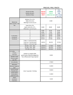


© Copyright 2026