
Introduction to Real Analysis by Lee Larson
Introduction to Real Analysis
Lee Larson
University of Louisville
February 5, 2015
About This Document
I often teach the MATH 501-502: Introduction to Real Analysis course at the
University of Louisville. These are notes I’ve compiled from those experiences. They
cover the basic ideas of analysis on the real line. The course is intended for a mix of
mostly senior mathematics majors and beginning graduate students.
The notes are updated quite often. The date of the version you’re reading is at
the bottom-left of most pages. The latest version is available for download at the
Web address math.louisville.edu/⇠lee/ira.
Feel free to use these notes for any purpose, as long as you give me blame or
credit. In return, I only ask you to tell me about mistakes. Also appreciated are
any suggestions and opinions. I can be contacted using the email address on the
Web page referenced above.
February 5, 2015
i
Contents
About This Document
i
Chapter 1. Basic Ideas
1. Sets
2. Algebra of Sets
3. Indexed Sets
4. Functions and Relations
5. Cardinality
6. Exercises
1-1
1-1
1-2
1-4
1-5
1-10
1-12
Chapter 2. The Real Numbers
1. The Field Axioms
2. The Order Axiom
3. The Completeness Axiom
4. Comparisons of Q and R
5. Exercises
2-1
2-1
2-3
2-5
2-8
2-10
Chapter 3. Sequences
1. Basic Properties
2. Monotone Sequences
3. Subsequences and the Bolzano-Weierstrass Theorem
4. Lower and Upper Limits of a Sequence
5. The Nested Interval Theorem
6. Cauchy Sequences
7. Exercises
3-1
3-1
3-4
3-6
3-7
3-9
3-9
3-12
Chapter 4. Series
1. What is a Series?
2. Positive Series
3. Absolute and Conditional Convergence
4. Rearrangements of Series
5. Exercises
4-1
4-1
4-3
4-10
4-12
4-15
Chapter 5. The Topology of R
1. Open and Closed Sets
2. Relative Topologies and Connectedness
3. Covering Properties and Compactness on R
4. More Small Sets
5. Exercises
5-1
5-1
5-4
5-5
5-8
5-13
Chapter 6.
Limits of Functions
6-1
i
1.
2.
3.
4.
5.
6.
7.
Basic Definitions
Unilateral Limits
Continuity
Unilateral Continuity
Continuous Functions
Uniform Continuity
Exercises
6-1
6-4
6-5
6-8
6-10
6-12
6-13
Chapter 7. Di↵erentiation
1. The Derivative at a Point
2. Di↵erentiation Rules
3. Derivatives and Extreme Points
4. Di↵erentiable Functions
5. Applications of the Mean Value Theorem
6. Exercises
7-1
7-1
7-2
7-5
7-6
7-9
7-14
Chapter 8. Integration
1. Partitions
2. Riemann Sums
3. Darboux Integration
4. The Integral
5. The Cauchy Criterion
6. Properties of the Integral
7. The Fundamental Theorem of Calculus
8. Change of Variables
9. Integral Mean Value Theorems
10. Exercises
8-1
8-1
8-2
8-4
8-7
8-9
8-10
8-13
8-16
8-19
8-20
Chapter 9. Sequences of Functions
1. Pointwise Convergence
2. Uniform Convergence
3. Metric Properties of Uniform Convergence
4. Series of Functions
5. Continuity and Uniform Convergence
6. Integration and Uniform Convergence
7. Di↵erentiation and Uniform Convergence
8. Power Series
9-1
9-1
9-3
9-5
9-6
9-6
9-11
9-13
9-15
Chapter 10. Fourier Series
1. Trigonometric Polynomials
2. The Riemann Lebesgue Lemma
3. The Dirichlet Kernel
4. Dini’s Test for Pointwise Convergence
5. The Fej´er Kernel
6. Fej´er’s Theorem
7. Exercises
Appendix.
Index
February 5, 2015
Bibliography
10-1
10-1
10-3
10-3
10-5
10-7
10-10
10-11
A-1
A-1
http://math.louisville.edu/⇠lee/ira
Appendix.
February 5, 2015
Index
A-2
http://math.louisville.edu/⇠lee/ira
CHAPTER 1
Basic Ideas
In the end, all mathematics can be boiled down to logic and set theory. Because
of this, any careful presentation of fundamental mathematical ideas is inevitably
couched in the language of logic and sets. This chapter defines enough of that
language to allow the presentation of basic real analysis. Much of it will be familiar
to you, but look at it anyway to make sure you understand the notation.
1. Sets
Set theory is a large and complicated subject in its own right. There is no time
in this course to touch on any but the simplest parts of it. Instead, we’ll just look
at a few topics from what is often called “naive set theory.”
We begin with a few definitions.
A set is a collection of objects called elements. Usually, sets are denoted by the
capital letters A, B, · · · , Z. A set can consist of any type and number of elements.
Even other sets can be elements of a set. The sets dealt with here usually have real
numbers as their elements.
If a is an element of the set A, we write a 2 A. If a is not an element of the set
A, we write a 2
/ A.
If all the elements of A are also elements of B, then A is a subset of B. In this
case, we write A ⇢ B or B A. In particular, notice that whenever A is a set, then
A ⇢ A.
Two sets A and B are equal, if they have the same elements. In this case we
write A = B. It is easy to see that A = B i↵ A ⇢ B and B ⇢ A. Establishing that
both of these containments are true is the most common way to show that two sets
are equal.
If A ⇢ B and A 6= B, then A is a proper subset of B. In cases when this is
important, it is written A ( B instead of just A ⇢ B.
There are several ways to describe a set.
A set can be described in words such as “P is the set of all presidents of the
United States.” This is cumbersome for complicated sets.
All the elements of the set could be listed in curly braces as S = {2, 0, a}. If
the set has many elements, this is impractical, or impossible.
More common in mathematics is set builder notation. Some examples are
P = {p : p is a president of the United states}
= {Washington, Adams, Je↵erson, · · · , Clinton, Bush, Obama}
and
A = {n : n is a prime number} = {2, 3, 5, 7, 11, · · · }.
1-1
1-2
CHAPTER 1. BASIC IDEAS
In general, the set builder notation defines a set in the form
{formula for a typical element : objects to plug into the formula}.
A more complicated example is the set of perfect squares:
S = {n2 : n is an integer} = {0, 1, 4, 9, · · · }.
The existence of several sets will be assumed. The simplest of these is the
empty set, which is the set with no elements. It is denoted as ;. The natural
numbers is the set N = {1, 2, 3, · · · } consisting of the positive integers. The set
Z = {· · · , 2, 1, 0, 1, 2, · · · } is the set of all integers. ! = {n 2 Z : n
0} =
{0, 1, 2, · · · } is the nonnegative integers. Clearly, ; ⇢ A, for any set A and
; ⇢ N ⇢ ! ⇢ Z.
Definition 1.1. Given any set A, the power set of A, written P(A), is the set
consisting of all subsets of A; i. e.,
P(A) = {B : B ⇢ A}.
For example, P({a, b}) = {;, {a}, {b}, {a, b}}. Also, for any set A, it is always
true that ; 2 P(A) and A 2 P(A). If a 2 A, it is never true that a 2 P(A), but it
is true that {a} ⇢ P(A). Make sure you understand why!
An amusing example is P(;) = {;}. (Don’t confuse ; with {;}! The former is
empty and the latter has one element.) Now, consider
P(;) = {;}
P(P(;)) = {;, {;}}
P(P(P(;))) = {;, {;}, {{;}}, {;, {;}}}
After continuing this n times, for some n 2 N, the resulting set,
P(P(· · · P(;) · · · )),
is very large. In fact, since a set with k elements has 2k elements in its power set,
22
there 22 = 65, 536 elements after only five iterations of the example. Beyond
this, the numbers are too large to print. Number sequences such as this one are
sometimes called tetrations.
2. Algebra of Sets
Let A and B be sets. There are four common binary operations used on sets.1
The union of A and B is the set containing all the elements in either A or B:
A [ B = {x : x 2 A _ x 2 B}.
The intersection of A and B is the set containing the elements contained in
both A and B:
A \ B = {x : x 2 A ^ x 2 B}.
1In the following, some logical notation is used. The symbol _ is the logical nonexclusive “or.”
The symbol ^ is the logical “and.” Their truth tables are as follows:
^
T
F
February 5, 2015
T
T
F
F
F
F
_
T
F
T
T
T
F
T
F
http://math.louisville.edu/⇠lee/ira
2. ALGEBRA OF SETS
1-3
A
A
B
A
B
A
B
A∆B
A\B
A
B
B
A
B
Figure 1. These are Venn diagrams showing the four standard binary
operations on sets. In this figure, the set which results from the operation
is shaded.
The di↵erence of A and B is the set of elements in A and not in B:
A \ B = {x : x 2 A ^ x 2
/ B}.
The symmetric di↵erence of A and B is the set of elements in one of the sets,
but not the other:
A B = (A [ B) \ (A \ B).
Another common set operation is complementation. The complement of a set A
is usually thought of as the set consisting of all elements which are not in A. But,
a little thinking will convice you this is not a meaningful definition because the
collection of elements not in A is not a precisely understood collection. To make
sense of the complement of a set, there must be a well-defined universal set U which
contains all the sets in question. Then the complement of a set A ⇢ U is Ac = U \ A.
It is usually the case that the universal set U is evident from the context in which
it is used.
With these operations, an extensive algebra for the manipulation of sets can
be developed. It’s usually done hand in hand with formal logic because the two
subjects share much in common. These topics are studied as part of Boolean algebra.
Several examples of set algebra are given in the following theorem and its corollary.
Theorem 1.2. Let A, B and C be sets.
(a) A \ (B [ C) = (A \ B) \ (A \ C)
(b) A \ (B \ C) = (A \ B) [ (A \ C)
February 5, 2015
http://math.louisville.edu/⇠lee/ira
1-4
CHAPTER 1. BASIC IDEAS
Proof. (a) This is proved as a sequence of equivalences.2
x 2 A \ (B [ C) () x 2 A ^ x 2
/ (B [ C)
() x 2 A ^ x 2
/ B^x2
/C
() (x 2 A ^ x 2
/ B) ^ (x 2 A ^ x 2
/ C)
() x 2 (A \ B) \ (A \ C)
(b) This is also proved as a sequence of equivalences.
x 2 A \ (B \ C) () x 2 A ^ x 2
/ (B \ C)
() x 2 A ^ (x 2
/ B_x2
/ C)
() (x 2 A ^ x 2
/ B) _ (x 2 A ^ x 2
/ C)
() x 2 (A \ B) [ (A \ C)
⇤
Theorem 1.2 is a version of a group of set equations which are often called
DeMorgan’s Laws. The more usual statement of DeMorgan’s Laws is in Corollary 1.3.
Corollary 1.3 is an obvious consequence of Theorem 1.2 when there is a universal
set to make the complementation well-defined.
Corollary 1.3 (DeMorgan’s Laws). Let A and B be sets.
(a) (A [ B)c = Ac \ B c
(b) (A \ B)c = Ac [ B c
3. Indexed Sets
We often have occasion to work with large collections of sets. For example, we
could have a sequence of sets A1 , A2 , A3 , · · · , where there is a set An associated
with each n 2 N. In general, let ⇤ be a set and suppose for each 2 ⇤ there is a set
A . The set {A : 2 ⇤} is called a collection of sets indexed by ⇤. In this case, ⇤
is called the indexing set for the collection.
Example 1.1. For each n 2 N, let An = {k 2 Z : k 2 n}. Then
A1 = A2 =A3 = { 1, 0, 1}, A4 = { 2, 1, 0, 1, 2}, · · · ,
A50 = { 7, 6, 5, 4, 3, 2, 1, 0, 1, 2, 3, 4, 5, 6, 7}, · · ·
is a collection of sets indexed by N.
Two of the basic binary operations can be extended to work with indexed
collections. In particular, using the indexed collection from the previous paragraph,
we define
[
A = {x : x 2 A for some 2 ⇤}
2⇤
and
\
2⇤
A = {x : x 2 A for all
2 ⇤}.
DeMorgan’s Laws can be generalized to indexed collections.
2The logical symbol () is the same as “if, and only if.” If A and B are any two statements,
then A () B is the same as saying A implies B and B implies A. It is also common to use i↵
in this way.
February 5, 2015
http://math.louisville.edu/⇠lee/ira
4. FUNCTIONS AND RELATIONS
then
Theorem 1.4. If {B :
1-5
2 ⇤} is an indexed collection of sets and A is a set,
A\
[
B =
A\
\
B =
and
2⇤
2⇤
\
(A \ B )
[
(A \ B ).
2⇤
2⇤
⇤
Proof. The proof of this theorem is Exercise 1.3.
4. Functions and Relations
4.1. Tuples. When listing the elements of a set, the order in which they are
listed is unimportant; e. g., {e, l, v, i, s} = {l, i, v, e, s}. If the order in which n items
are listed is important, the list is called an n-tuple. (Strictly speaking, an n-tuple is
not a set.) We denote an n-tuple by enclosing the ordered list in parentheses. For
example, if x1 , x2 , x3 , x4 are 4 items, the 4-tuple (x1 , x2 , x3 , x4 ) is di↵erent from the
4-tuple (x2 , x1 , x3 , x4 ).
Because they are used so often, 2-tuples are called ordered pairs and a 3-tuple
is called an ordered triple.
Definition 1.5. The Cartesian product of two sets A and B is the set of all
ordered pairs
A ⇥ B = {(a, b) : a 2 A ^ b 2 B}.
Example 1.2. If A = {a, b, c} and B = {1, 2}, then
A ⇥ B = {(a, 1), (a, 2), (b, 1), (b, 2), (c, 1), (c, 2)}.
and
B ⇥ A = {(1, a), (1, b), (1, c), (2, a), (2, b), (2, c)}.
Notice that A ⇥ B 6= B ⇥ A because of the importance of order in the ordered pairs.
A useful way to visualize the Cartesian product of two sets is as a table. The
Cartesian product A ⇥ B from Example 1.2 is listed as the entries of the following
table.
1
2
a (a, 1) (a, 2)
b (b, 1) (b, 2)
c (c, 1) (c, 2)
Of course, the common Cartesian plane from your analytic geometry course is
nothing more than a generalization of this idea of listing the elements of a Cartesian
product as a table.
The definition of Cartesian product can be extended to the case of more than
two sets. If {A1 , A2 , · · · , An } are sets, then
A1 ⇥ A2 ⇥ · · · ⇥ An = {(a1 , a2 , · · · , an ) : ak 2 Ak for 1 k n}
is a set of n-tuples. This is often written as
n
Y
k=1
February 5, 2015
Ak = A1 ⇥ A2 ⇥ · · · ⇥ An .
http://math.louisville.edu/⇠lee/ira
1-6
CHAPTER 1. BASIC IDEAS
4.2. Relations.
Definition 1.6. If A and B are sets, then any R ⇢ A ⇥ B is a relation from A
to B. If (a, b) 2 R, we write aRb.
In this case,
dom (R) = {a : (a, b) 2 R}
is the domain of R and
is the range of R.
ran (R) = {b : (a, b) 2 R}
In the special case when R ⇢ A ⇥ A, for some set A, there is some additional
terminology.
R is symmetric, if aRb () bRa.
R is reflexive, if aRa whenever a 2 dom (A).
R is transitive, if aRb ^ bRc =) aRc.
R is an equivalence relation on A, if it is symmetric, reflexive and transitive.
Example 1.3. Let R be the relation on Z ⇥ Z defined by aRb () a b.
Then R is reflexive and transitive, but not symmetric.
Example 1.4. Let R be the relation on Z ⇥ Z defined by aRb () a < b.
Then R is transitive, but neither reflexive nor symmetric.
Example 1.5. Let R be the relation on Z ⇥ Z defined by aRb () a2 = b2 .
In this case, R is an equivalence relation. It is evident that aRb i↵ b = a or b = a.
4.3. Functions.
Definition 1.7. A relation R ⇢ A ⇥ B is a function if
aRb1 ^ aRb2 =) b1 = b2 .
If f ⇢ A ⇥ B is a function and dom (f ) = A, then we usually write f : A ! B
and use the usual notation f (a) = b instead of af b.
If f : A ! B is a function, the usual intuitive interpretation is to regard f
as a rule that associates each element of A with a unique element of B. It’s not
necessarily the case that each element of B is associated with something from A;
i.e., B may not be ran (f ).
Example 1.6. Define f : N ! Z by f (n) = n2 and g : Z ! Z by g(n) = n2 .
In this case ran (f ) = {n2 : n 2 N} and ran (g) = ran (f ) [ {0}. Notice that even
though f and g use the same formula, they are actually di↵erent functions.
Definition 1.8. If f : A ! B and g : B ! C, then the composition of g with
f is the function g f : A ! C defined by g f (a) = g(f (a)).
In Example 1.6, g f (n) = g(f (n)) = g(n2 ) = (n2 )2 = n4 makes sense for all
n 2 N, but f g is undefined at n = 0.
There are several important types of functions.
Definition 1.9. A function f : A ! B is a constant function, if ran (f ) has a
single element; i. e., there is a b 2 B such that f (a) = b for all a 2 A. The function
f is surjective (or onto B), if ran (f ) = B.
February 5, 2015
http://math.louisville.edu/⇠lee/ira
4. FUNCTIONS AND RELATIONS
1-7
f
b
a
c
f
B
A
f
g
b
a
c
g
B
A
g
Figure 2. These diagrams show two functions, f : A ! B and g : A !
B. The function g is injective and f is not because f (a) = f (c).
In a sense, constant and surjective functions are the opposite extremes. A
constant function has the smallest possible range and a surjective function has the
largest possible range. Of course, a function f : A ! B can be both constant and
surjective, if B has only one element.
Definition 1.10. A function f : A ! B is injective (or one-to-one), if
f (a) = f (b) implies a = b.
The terminology “one-to-one” is very descriptive because such a function
uniquely pairs up the elements of its domain and range. An illustration of this
definition is in Figure 2. In Example 1.6, f is injective while g is not.
Definition 1.11. A function f : A ! B is bijective, if it is both surjective and
injective.
A bijective function can be visualized as uniquely pairing up all the elements of
A and B. Some authors, favoring less pretentious language, use the more descriptive
terminology one-to-one correspondence instead of bijection. This pairing up of the
elements from each set is like counting them and finding they have the same number
of elements. Given any two sets, no matter how many elements they have, the
intuitive idea is they have the same number of elements if, and only if, there is a
bijection between them.
The following theorem shows that this property of counting the number of
elements works in a familiar way. (Its proof is left as an easy exercise.)
Theorem 1.12. If f : A ! B and g : B ! C are bijections, then g f : A ! C
is a bijection.
4.4. Inverse Functions.
February 5, 2015
http://math.louisville.edu/⇠lee/ira
1-8
CHAPTER 1. BASIC IDEAS
f
f
—1
f —1
A
f
B
Figure 3. This is one way to visualize a general invertible function.
First f does something to a and then f
1
undoes it.
Definition 1.13. If f : A ! B, C ⇢ A and D ⇢ B, then the image of C is the
set f (C) = {f (a) : a 2 C}. The inverse image of D is the set f 1 (D) = {a : f (a) 2
D}.
Definitions 1.11 and 1.13 work together in the following way. Suppose f : A ! B
is bijective and b 2 B. The fact that f is surjective guarantees that f 1 ({b}) 6= ;.
Since f is injective, f 1 ({b}) contains only one element, say a, where f (a) = b. In
this way, it is seen that f 1 is a rule that assigns each element of B to exactly one
element of A; i. e., f 1 is a function with domain B and range A.
Definition 1.14. If f : A ! B is bijective, the inverse of f is the function
f 1 : B ! A with the property that f 1 f (a) = a for all a 2 A and f f 1 (b) = b
for all b 2 B.
There is some ambiguity in the meaning of f 1 between 1.13 and 1.14. The
former is an operation working with subsets of A and B; the latter is a function
working with elements of A and B. It’s usually clear from the context which meaning
is being used.
Example 1.7. Let A = N and B be the even natural numbers. If f : A ! B
is f (n) = 2n and g : B ! A is g(n) = n/2, it is clear f is bijective. Since
f g(n) = f (n/2) = 2n/2 = n and g f (n) = g(2n) = 2n/2 = n, we see g = f 1 .
(Of course, it is also true that f = g 1 .)
Example 1.8. Let f : N ! Z be defined by
(
(n 1)/2, n odd,
f (n) =
n/2,
n even
It’s quite easy to see that f is bijective and
(
2n + 1,
1
f (n) =
2n,
n 0,
n<0
Given any set A, it’s obvious there is a bijection f : A ! A and, if g : A ! B is a
bijection, then so is g 1 : B ! A. Combining these observations with Theorem 1.12,
an easy theorem follows.
Theorem 1.15. Let S be a collection of sets. The relation on S defined by
A ⇠ B () there is a bijection f : A ! B
is an equivalence relation.
February 5, 2015
http://math.louisville.edu/⇠lee/ira
4. FUNCTIONS AND RELATIONS
1-9
4.5. Schr¨
oder-Bernstein Theorem. The following theorem is a powerful
tool in set theory, and shows that a seemingly intuitively obvious statement is
sometimes difficult to verify. It will be used in Section 5.
Theorem 1.16 (Schr¨oder-Bernstein3). Let A and B be sets. If there are injective
functions f : A ! B and g : B ! A, then there is a bijective function h : A ! B.
A
A1
B1
A3
A2
B3
B2
A4
A5
B5
B4
f (A)
···
···
B
Figure 4. Here are the first few steps from the construction used in
the proof of Theorem 1.16.
Proof. Let B1 = B\f (A). If Bk ⇢ B is defined for some k 2 N, let Ak = g(Bk )
and Bk+1 = f (Ak ). This inductively defines Ak and Bk for all k 2 N. Use these
S
sets to define A˜ = k2N Ak and h : A ! B as
(
g 1 (x), x 2 A˜
h(x) =
.
f (x),
x 2 A \ A˜
It must be shown that h is well-defined, injective and surjective.
˜ then it is clear h(x) = f (x) is
To show h is well-defined, let x 2 A. If x 2 A \ A,
˜
defined. On the other hand, if x 2 A, then x 2 Ak for some k. Since x 2 Ak = g(Bk ),
we see h(x) = g 1 (x) is defined. Therefore, h is well-defined.
To show h is injective, let x, y 2 A with x 6= y.
˜ then the assumptions that g and f are injective,
If both x, y 2 A˜ or x, y 2 A \ A,
respectively, imply h(x) 6= h(y).
˜ Suppose x 2 Ak and
The remaining case is when x 2 A˜ and y 2 A \ A.
h(x) = h(y). If k = 1, then h(x) = g 1 (x) 2 B1 and h(y) = f (y) 2 f (A) = B \ B1 .
This is clearly incompatible with the assumption that h(x) = h(y). Now, suppose
k > 1. Then there is an x1 2 B1 such that
x=g f
|
k
This implies
h(x) = g
1
g f ··· f
{z
1 f ’s and k g’s
(x) = f
|
k
g f
··· f
{z
1 f ’s and k
g (x1 ).
}
g (x1 ) = f (y)
}
1 g’s
3
This is often called the Cantor-Schr¨
oder-Bernstein or Cantor-Bernstein Theorem, despite the
fact that it was apparently first proved by Richard Dedekind.
February 5, 2015
http://math.louisville.edu/⇠lee/ira
1-10
CHAPTER 1. BASIC IDEAS
so that
y=g f
|
k
g f ··· f
{z
2 f ’s and k
1 g’s
g (x1 ) 2 Ak
}
1
˜
⇢ A.
This contradiction shows that h(x) 6= h(y). We conclude h is injective.
To show h is surjective, let y 2 B. If y 2 Bk for some k, then h(Ak ) = g 1 (Ak ) =
Bk shows y 2 h(A). If y 2
/ Bk for any k, y 2 f (A) because B1 = B \ f (A), and
˜ so y = h(x) = f (x) for some x 2 A. This shows h is surjective.
g(y) 2
/ A,
⇤
The Schr¨oder-Bernstein theorem has many consequences, some of which are at
first a bit unintuitive, such as the following theorem.
Corollary 1.17. There is a bijective function h : N ! N ⇥ N
Proof. If f : N ! N ⇥ N is f (n) = (n, 1), then f is clearly injective. On the
other hand, suppose g : N ⇥ N ! N is defined by g((a, b)) = 2a 3b . The uniqueness
of prime factorizations guarantees g is injective. An application of Theorem 1.16
yields h.
⇤
To appreciate the power of the Schr¨oder-Bernstein theorem, try to find an
explicit bijection h : N ! N ⇥ N.
5. Cardinality
There is a way to use sets and functions to formalize and generalize how we
count. For example, suppose we want to count how many elements are in the set
{a, b, c}. The natural way to do this is to point at each element in succession and
say “one, two, three.” What is really happening is that we’re defining a bijective
function between {a, b, c} and the set {1, 2, 3}. This idea can be generalized.
Definition 1.18. Given n 2 N, the set n = {1, 2, · · · , n} is called an initial
segment of N. The trivial initial segment is 0 = ;. A set S has cardinality n, if
there is a bijective function f : S ! n. In this case, we write card (S) = n.
The cardinalities defined in Definition 1.18 are called the finite cardinal numbers.
They correspond to the everyday counting numbers we usually use. The idea can
be generalized still further.
Definition 1.19. Let A and B be two sets. If there is an injective function
f : A ! B, we say card (A) card (B).
According to Theorem 1.16, the Schr¨oder-Bernstein Theorem, if card (A)
card (B) and card (B) card (A), then there is a bijective function f : A ! B. As
expected, in this case we write card (A) = card (B). When card (A) card (B), but
no such bijection exists, we write card (A) < card (B). Theorem 1.15 shows that
card (A) = card (B) is an equivalence relation between sets.
The idea here, of course, is that card (A) = card (B) means A and B have the
same number of elements and card (A) < card (B) means A is a smaller set than B.
This simple intuitive understanding has some surprising consequences when the sets
involved do not have finite cardinality.
In particular, the set A is countably infinite, if card (A) = card (N). In this case,
it is common to write card (N) = @0 .4 When card (A) @0 , then A is said to be a
4The symbol @ is the Hebrew letter “aleph” and @ is usually pronounced “aleph nought.”
0
February 5, 2015
http://math.louisville.edu/⇠lee/ira
5. CARDINALITY
1-11
countable set. In other words, the countable sets are those having finite or countably
infinite cardinality.
Example 1.9. Let f : N ! Z be defined as
(
n+1
when n is odd
2 ,
f (n) =
.
n
1 2 , when n is even
It’s easy to show f is a bijection, so card (N) = card (Z) = @0 .
Theorem 1.20. Suppose A and B are countable sets.
(a) A ⇥ B is countable.
(b) A [ B is countable.
Proof. (a) This is a consequence of Theorem 1.17.
(b) This is Exercise 1.20.
⇤
An alert reader will have noticed from previous examples that
@0 = card (Z) = card (!) = card (N) = card (N ⇥ N) = card (N ⇥ N ⇥ N) = · · ·
A logical question is whether all sets either have finite cardinality, or are countably
infinite. That this is not so is seen by letting S = N in the following theorem.
Theorem 1.21. If S is a set, card (S) < card (P(S)).
Proof. Noting that 0 = card (;) < 1 = card (P(;)), the theorem is true when
S is empty.
Suppose S 6= ;. Since {a} 2 P(S) for all a 2 S, it follows that card (S)
card (P(S)). Therefore, it suffices to prove there is no surjective function f : S !
P(S).
To see this, assume there is such a function f and let T = {x 2 S : x 2
/ f (x)}.
Since f is surjective, there is a t 2 S such that f (t) = T . Either t 2 T or t 2
/ T.
If t 2 T = f (t), then the definition of T implies t 2
/ T , a contradiction. On
the other hand, if t 2
/ T = f (t), then the definition of T implies t 2 T , another
contradiction. These contradictions lead to the conclusion that no such function f
can exist.
⇤
A set S is said to be uncountably infinite, or just uncountable, if @0 < card (S).
Theorem 1.21 implies @0 < card (P(N)), so P(N) is uncountable. In fact, the same
argument implies
@0 = card (N) < card (P(N)) < card (P(P(N))) < · · ·
So, there are an infinite number of distinct infinite cardinalities.
In 1874 Georg Cantor [5] proved card (R) = card (P(N)) and card (R) > @0 ,
where R is the set of real numbers. (A version of Cantor’s theorem appears in
Theorem 2.25 below.) This naturally led to the question whether there are sets S
such that @0 < card (S) < card (R). Cantor spent many years trying answer this
question and never succeeded. His assumption that no such sets exist came to be
called the continuum hypothesis.
The importance of the continuum hypothesis was highlighted by David Hilbert
at the 1900 International Congress of Mathematicians in Paris, when he put it first
on his famous list of the 23 most important open problems in mathematics. Kurt
G¨odel proved in 1940 that the continuum hypothesis cannot be disproved using
February 5, 2015
http://math.louisville.edu/⇠lee/ira
1-12
CHAPTER 1. BASIC IDEAS
standard set theory, but he did not prove it was true. In 1963 it was proved by
Paul Cohen that the continuum hypothesis is actually unprovable as a theorem in
standard set theory.
So, the continuum hypothesis is a statement with the strange property that it
is neither true nor false within the framework of ordinary set theory. This means
that in the standard axiomatic development of set theory, the continuum hypothesis,
or a suitable negation of it, can be taken as an additional axiom without causing
any contradictions. The technical terminology is that the continuum hypothesis is
independent of the axioms of set theory.
The proofs of these theorems are extremely difficult and entire broad areas of
mathematics were invented just to make their proofs possible. Even today, there
are some deep philosophical questions swirling around them. A more technical
introduction to many of these ideas is contained in the book by Ciesielski [7].
A nontechnical and very readable history of the e↵orts by mathematicians to
understand the continuum hypothesis is the book by Aczel [1].
6. Exercises
1.1. If a set S has n elements for n 2 !, then how many elements are in P(S)?
1.2. Prove that for any sets A and B,
(a) A = (A \ B) [ (A \ B)
(b) A [ B = (A \ B) [ (B \ A) [ (A \ B) and that the sets A \ B, B \ A and
A \ B are pairwise disjoint.
(c) A \ B = A \ B c .
1.3. Prove Theorem 1.4.
1.4. For any sets A, B, C and D,
(A ⇥ B) \ (C ⇥ D) = (A \ C) ⇥ (B \ D)
and
(A ⇥ B) [ (C ⇥ D) ⇢ (A [ C) ⇥ (B [ D).
Why does equality not hold in the second expression?
1.5. Prove Theorem 1.15.
1.6. Suppose R is an equivalence relation on A. For each x 2 A define Cx =
{y 2 A : xRy}. Prove that if x, y 2 A, then either Cx = Cy or Cx \ Cy = ;. (The
collection {Cx : x 2 A} is the set of equivalence classes induced by R.)
1.7. If f : A ! B and g : B ! C are bijections, then so is g f : A ! C.
1.8. Prove or give a counter example: f : X ! Y is injective i↵ whenever A and
B are disjoint subsets of Y , then f 1 (A) \ f 1 (B) = ;.
1.9. If f : A ! B is bijective, then f
1
is unique.
1.10. Prove that f : X ! Y is surjective i↵ for each subset A ⇢ X, Y \ f (A) ⇢
f (X \ A).
February 5, 2015
http://math.louisville.edu/⇠lee/ira
6. EXERCISES
1-13
1.11. Suppose that Ak is a set for each positive integer k.
T 1 S1
(a) Show that x 2 Sn=1 (Tk=n Ak ) i↵ x 2 Ak for infinitely many sets Ak .
1
1
(b) Show that x 2 n=1 ( k=n Ak ) i↵ x 2 Ak for all but finitely many of the
sets Ak .
T1 S 1
The S
set n=1
T1( k=n Ak ) from (a) is often called the superior limit of the sets Ak
1
and n=1 ( k=n Ak ) is often called the inferior limit of the sets Ak .
B
1.12. Given two sets A and B, it is common to let
⇣ A
⌘ denote the set of all
A
functions f : B ! A. Prove that for any set A, card 2
= card (P(A)). This is
why many authors use 2A as their notation for P(A).
1.13. Let S be a set. Prove the following two statements are equivalent:
(a) S is infinite; and,
(b) there is a proper subset T of S and a bijection f : S ! T .
This statement is often used as the definition of when a set is infinite.
1.14. If S is an infinite set, then there is a countably infinite
collection of nonempty
S
pairwise disjoint infinite sets Tn , n 2 N such that S = n2N Tn .
1.15. Without using the Schr¨oder-Bernstein theorem, find a bijection f : [0, 1] !
(0, 1).
1.16. If f : [0, 1) ! (0, 1) and g : (0, 1) ! [0, 1) are given by f (x) = x + 1 and
g(x) = x, then the proof of the Schr˘oder-Bernstein theorem yields what bijection
h : [0, 1) ! (0, 1)?
1.17. Find a function f : R \ {0} ! R \ {0} such that f
1
= 1/f .
1.18. Find a bijection f : [0, 1) ! (0, 1).
1.19. If f : A ! B and g : B ! A are functions such that f
x 2 B and g f (x) = x for all x 2 A, then f 1 = g.
g(x) = x for all
1.20. If A and B are sets such that card (A) = card (B) = @0 , then card (A [ B) =
@0 .
1.21. Using the notation from the proof of the Schr¨oder-Bernstein Theorem, let
A = [0, 1), B = (0, 1), f (x) = x + 1 and g(x) = x. Determine h(x).
1.22. Using the notation from the proof of the Schr¨oder-Bernstein Theorem, let
A = N, B = Z, f (n) = n and
(
1 3n, n 0
g(n) =
.
3n 1, n > 0
Calculate h(6) and h(7).
1.23. Suppose that in the statement of the Schr¨oder-Bernstein theorem A = B = Z
and f (n) = g(n) = 2n. Following the procedure in the proof yields what function h?
February 5, 2015
http://math.louisville.edu/⇠lee/ira
1-14
CHAPTER 1. BASIC IDEAS
1.24. If {An : n 2 N} is a collection of countable sets, then
S
n2N
An is countable.
1.25. If A and B are sets, the set
⇣ of⌘all functions f : A ! B is often denoted by
S
B A . If S is a set, prove that card 2 = card (P(S)).
1.26. If @0 card (S)), then there is an injective function f : S ! S that is not
surjective.
1.27. If card (S) = @0 , then there is a sequence
S of pairwise disjoint sets Tn , n 2 N
such that card (Tn ) = @0 for every n 2 N and n2N Tn = S.
February 5, 2015
http://math.louisville.edu/⇠lee/ira
CHAPTER 2
The Real Numbers
This chapter concerns what can be thought of as the rules of the game: the
axioms of the real numbers. These axioms imply all the properties of the real
numbers and, in a sense, any set satisfying them is uniquely determined to be the
real numbers.
The axioms are presented here as rules without very much justification. Other
approaches can be used. For example, a common approach is to begin with the
Peano axioms — the axioms of the natural numbers — and build up to the real
numbers through several “completions” of the natural numbers. It’s also possible to
begin with the axioms of set theory to build up the Peano axioms as theorems and
then use those to prove our axioms as further theorems. No matter how it’s done,
there are always some axioms at the base of the structure and the rules for the real
numbers are the same, whether they’re axioms or theorems.
We choose to start at the top because the other approaches quickly turn into
a long and tedious labyrinth of technical exercises without much connection to
analysis.
1. The Field Axioms
These first six axioms are called the field axioms because any object satisfying
them is called a field. They give the algebraic properties of the real numbers.
A field is a nonempty set F along with two binary operations, multiplication
⇥ : F ⇥ F ! F and addition + : F ⇥ F ! F satisfying the following axioms.1
Axiom 1 (Associative Laws). If a, b, c 2 F, then (a + b) + c = a + (b + c) and
(a ⇥ b) ⇥ c = a ⇥ (b ⇥ c).
Axiom 2 (Commutative Laws). If a, b 2 F, then a + b = b + a and a ⇥ b = b ⇥ a.
Axiom 3 (Distributive Law). If a, b, c 2 F, then a ⇥ (b + c) = (a ⇥ b) + (a ⇥ c).
Axiom 4 (Existence of identities). There are 0, 1 2 F such that a + 0 = a and
a ⇥ 1 = a, for all a 2 F.
Axiom 5 (Existence of an additive inverse). For each a 2 F there is
such that a + ( a) = 0.
a2F
1Given a set A, a function f : A ⇥ A ! A is called a binary operation. In other words, a
binary operation is just a function with two arguments. The standard notations of +(a, b) = a + b
and ⇥(a, b) = a ⇥ b are used here. The symbol ⇥ is unfortunately used for both the Cartesian
product and the field operation, but the context in which it’s used removes the ambiguity.
2-1
2-2
a
1
CHAPTER 2. THE REAL NUMBERS
Axiom 6 (Existence of a multiplicative inverse). For each a 2 F \ {0} there is
2 F such that a ⇥ a 1 = 1.
Although these axioms seem to contain most properties of the real numbers we
normally use, they don’t characterize the real numbers; they just give the rules for
arithmetic. There are other fields besides the real numbers and studying them is a
large part of most abstract algebra courses.
Example 2.1. From elementary algebra we know that the rational numbers
Q = {p/q : p 2 Z ^ q 2 N}
p
form a field. It is shown in Theorem 2.12 that 2 2
/ Q, so Q doesn’t contain all the
real numbers.
Example 2.2. Let F = {0, 1, 2} with addition and multiplication calculated
modulo 3. The addition and multiplication tables are as follows.
+
0
1
2
0
0
1
2
1
1
2
0
2
2
0
1
⇥
0
1
2
0
0
0
0
1
0
1
2
2
0
2
1
It is easy to check that the field axioms are satisfied. This field is usually called Z3 .
The following theorems, containing just a few useful properties of fields, are
presented mostly as examples showing how the axioms are used. More complete
developments can be found in any beginning abstract algebra text.
Theorem 2.1. The additive and multiplicative identities of a field F are unique.
Proof. Suppose e1 and e2 are both multiplicative identities in F. Then
e1 = e1 ⇥ e2 = e2 ,
so the multiplicative identity is unique. The proof for the additive identity is
essentially the same.
⇤
Theorem 2.2. Let F be a field. If a, b 2 F with b 6= 0, then
unique.
a and b
1
are
Proof. Suppose b1 and b2 are both multiplicative inverses for b 6= 0. Then,
using Axioms 4 and 1,
b1 = b1 ⇥ 1 = b1 ⇥ (b ⇥ b2 ) = (b1 ⇥ b) ⇥ b2 = 1 ⇥ b2 = b2 .
This shows the multiplicative inverse in unique. The proof is essentially the same
for the additive inverse.
⇤
There are many other properties of fields which could be proved here, but they
correspond to the usual properties of the real numbers learned in beginning algebra,
so we omit them. Some of them are in the exercises at the end of this chapter.
From now on, the standard notations for algebra will usually be used; e. g., we
will allow ab instead of a ⇥ b and a/b instead of a ⇥ b 1 . The reader may also use
the standard facts she learned from elementary algebra.
February 5, 2015
http://math.louisville.edu/⇠lee/ira
2. THE ORDER AXIOM
2-3
2. The Order Axiom
The axiom of this section gives the order and metric properties of the real
numbers. In a sense, the following axiom adds some geometry to a field.
Axiom 7 (Order axiom.). There is a set P ⇢ F such that
(a) If a, b 2 P , then a + b, ab 2 P .
(b) If a 2 F, then exactly one of the following is true: a 2 P ,
a = 0.
a 2 P or
Any field F satisfying the axioms so far listed is naturally called an ordered field.
Of course, the set P is known as the set of positive elements of F. Using Axiom 7(ii),
we see that F is divided into three pairwise disjoint sets: P , {0} and { x : x 2 P }.
The latter of these is, of course, the set of negative elements from F. The following
definition introduces familiar notation for order.
Definition 2.3. We write a < b or b > a, if b
and b a are now as expected.
a 2 P . The meanings of a b
Notice that a > 0 () a = a 0 2 P and a < 0 () a = 0 a 2 P , so
a > 0 and a < 0 agree with our usual notions of positive and negative.
Our goal is to capture all the properties of the real numbers with the axioms.
The order axiom eliminates many fields from consideration. For example, Exercise
2.5 shows the field Z3 of Example 2.2 is not an ordered field. On the other hand,
facts from elementary algebra imply Q is an ordered field, so the first seven axioms
still don’t “capture” the real numbers.
Following are a few standard properties of ordered fields.
Theorem 2.4. Let F be an ordered field and a 2 F. a 6= 0 i↵ a2 > 0.
Proof. ()) If a > 0, then a2 > 0 by Axiom 7(a). If a < 0, then
Axiom 7(b) and a2 = 1a2 = ( 1)( 1)a2 = ( a)2 > 0.
(() Since 02 = 0, this is obvious.
a > 0 by
⇤
Theorem 2.5. If F is an ordered field and a, b, c 2 F, then
(a) a < b () a + c < b + c,
(b) a < b ^ b < c =) a < c,
(c) a < b ^ c > 0 =) ac < bc,
(d) a < b ^ c < 0 =) ac > bc.
Proof. (a) a < b () b a 2 P () (b + c) (a + c) 2 P () a + c < b + c.
(b) By supposition, both b a, c b 2 P . Using the fact that P is closed under
addition, we see (b a) + (c b) = c a 2 P . Therefore, c > a.
(c) Since b a 2 P and c 2 P and P is closed under multiplication, c(b a) =
cb ca 2 P and, therefore, ac < bc.
(d) By assumption, b a, c 2 P . Apply part (c) and Exercise 2.1.
⇤
Theorem 2.6 (Two Out of Three Rule). Let F be an ordered field and a, b, c 2 F.
If ab = c and any two of a, b or c are positive, then so is the third.
Proof. If a > 0 and b > 0, then Axiom 7(a) implies c > 0. Next, suppose
a > 0 and c > 0. In order to force a contradiction, suppose b 0. In this case,
Axiom 7(b) shows
0 a( b) = (ab) = c < 0,
which is impossible.
⇤
February 5, 2015
http://math.louisville.edu/⇠lee/ira
2-4
CHAPTER 2. THE REAL NUMBERS
Corollary 2.7. Let F be an ordered field and a 2 F. If a > 0, then a
If a < 0, then a 1 < 0.
1
> 0.
⇤
Proof. The proof is Exercise 2.2.
Suppose a > 0. Since 1a = a, Theorem 2.6 implies 1 > 0. Applying Theorem
2.5, we see that 1 + 1 > 1 > 0. It’s clear that by induction, we can find a copy of N
embedded in any ordered field. Similarly, Z and Q also have unique copies in any
ordered field.
The standard notation for intervals will be used on an ordered field, F; i. e.,
(a, b) = {x 2 F : a < x < b}, (a, 1) = {x 2 F : a < x}, [a, b] = {x 2 F : a x b},
etc. It’s also useful to start visualizing F as a standard number line.
2.1. Metric Properties. The order axiom on a field F allows us to introduce
the idea of the distance between points in F. To do this, we begin with the following
familiar definition.
Definition 2.8. Let F be an ordered field. The absolute value function on F is
a function | · | : F ! F defined as
(
x,
x 0
|x| =
.
x, x < 0
The most important properties of the absolute value function are contained in
the following theorem.
Theorem 2.9. Let F be an ordered field and x, y 2 F. Then
(a) |x| 0 and |x| = 0 () x = 0;
(b) |x| = | x|;
(c) |x| x |x|;
(d) |x| y () y x y; and,
(e) |x + y| |x| + |y|.
Proof.
(a) The fact that |x| 0 for all x 2 F follows from Axiom 7(b).
Since 0 = 0, the second part is clear.
(b) If x 0, then x 0 so that | x| = ( x) = x = |x|. If x < 0, then
x > 0 and |x| = x = | x|.
(c) If x 0, then |x| = x x = |x|. If x < 0, then |x| = ( x) = x <
x = |x|.
(d) This is left as Exercise 2.3.
(e) Add the two sets of inequalities |x| x |x| and |y| y |y| to see
(|x| + |y|) x + y |x| + |y|. Now apply (d).
⇤
From studying analytic geometry and calculus, we are used to thinking of |x y|
as the distance between the numbers x and y. This notion of a distance between
two points of a set can be generalized.
Definition 2.10. Let S be a set and d : S ⇥ S ! R satisfy
(a) for all x, y 2 S, d(x, y) 0 and d(x, y) = 0 () x = y,
(b) for all x, y 2 S, d(x, y) = d(y, x), and
(c) for all x, y, z 2 S, d(x, z) d(x, y) + d(y, z).
Then the function d is a metric on S. The pair (S, d) is called a metric space.
February 5, 2015
http://math.louisville.edu/⇠lee/ira
3. THE COMPLETENESS AXIOM
2-5
A metric is a function which defines the distance between any two points of a
set.
Example 2.3. Let S be a set and define d : S ⇥ S ! S by
(
1, x 6= y
d(x, y) =
.
0, x = y
It can readily be verified that d is a metric on S. This simplest of all metrics is
called the discrete metric and it can be defined on any set. It’s not often useful.
Theorem 2.11. If F is an ordered field, then d(x, y) = |x
Proof. Use parts (a), (b) and (e) of Theorem 2.9.
y| is a metric on F.
⇤
The metric on F derived from the absolute value function is called the standard
metric on F. There are other metrics sometimes defined for specialized purposes,
but we won’t have need of them.
3. The Completeness Axiom
All the axioms given so far are obvious from beginning algebra, and, on the
surface, it’s not obvious they haven’t captured all the properties of the real numbers.
Since Q satisfies them all, the following theorem shows that we’re not yet done.
Theorem 2.12. There is no ↵ 2 Q such that ↵2 = 2.
Proof. Assume to the contrary that there is ↵ 2 Q with ↵2 = 2. Then there
are p, q 2 N such that ↵ = p/q with p and q relatively prime. Now,
✓ ◆2
p
(4)
= 2 =) p2 = 2q 2
q
shows p2 is even. Since the square of an odd number is odd, p must be even; i. e.,
p = 2r for some r 2 N. Substituting this into (4), shows 2r2 = q 2 . The same
argument as above establishes q is also even. This contradicts the assumption that
p and q are relatively prime. Therefore, no such ↵ exists.
⇤
p
Since we suspect 2 is a perfectly fine number, there’s still something missing
from the list of axioms. Completeness is the missing idea.
The Completeness Axiom is somewhat more complicated than the previous
axioms, and several definitions are needed in order to state it.
3.1. Bounded Sets.
Definition 2.13. A subset S of an ordered field F is bounded above, if there
exists M 2 F such that M
x for all x 2 S. A subset S of an ordered field F is
bounded below, if there exists m 2 F such that m x for all x 2 S. The elements
M and m are called an upper bound and lower bound for S, respectively. If S is
bounded both above and below, it is a bounded set.
There is no requirement in the definition that the upper and lower bounds for a
set are elements of the set. They can be elements of the set, but typically are not.
For example, if N = ( 1, 0), then [0, 1) is the set of all upper bounds for N , but
none of them is in N . On the other hand, if T = ( 1, 0], then [0, 1) is again the
set of all upper bounds for T , but in this case 0 is an upper bound which is also an
February 5, 2015
http://math.louisville.edu/⇠lee/ira
2-6
CHAPTER 2. THE REAL NUMBERS
element of T . An extreme case is ;. A vacuous argument shows every element of F
is both an upper and lower bound, but obviously none of them is in ;.
A set need not have upper or lower bounds. For example N = ( 1, 0) has no
lower bounds, while P = (0, 1) has no upper bounds. The integers, Z, has neither
upper nor lower bounds. If S has no upper bound, it is unbounded above and, if
it has no lower bound, then it is unbounded below. In either case, it is usually just
said to be unbounded.
If M is an upper bound for the set S, then every x M is also an upper bound
for S. Considering some simple examples should lead you to suspect that among
the upper bounds for a set, there is one that is best in the sense that everything
greater is an upper bound and everything less is not an upper bound. This is the
basic idea of completeness.
Definition 2.14. Suppose F is an ordered field and S is bounded above in F.
A number B 2 F is called a least upper bound of S if
(a) B is an upper bound for S, and
(b) if ↵ is any upper bound for S, then B ↵.
If S is bounded below in F, then a number b 2 F is called a greatest lower bound of
S if
(a) b is a lower bound for S, and
(b) if ↵ is any lower bound for S, then b ↵.
Theorem 2.15. If F is an ordered field and A ⇢ F is nonempty, then A has at
most one least upper bound and at most one greatest lower bound.
Proof. Suppose u1 and u2 are both least upper bounds for A. Since u1 and
u2 are both upper bounds for A, u1 u2 u1 =) u1 = u2 . The proof of the
other case is similar.
⇤
Definition 2.16. If A ⇢ F is nonempty and bounded above, then the least
upper bound of A is written lub A. When A is not bounded above, we write
lub A = 1. When A = ;, then lub A = 1.
If A ⇢ F is nonempty and bounded below, then the greatest lower of A is
written glb A. When A is not bounded below, we write glb A = 1. When A = ;,
then glb A = 1.2
Notice that the symbol “1” is not an element of F. Writing lub A = 1 is just
a convenient way to say A has no upper bounds. Similarly lub ; = 1 tells us ;
has every real number as an upper bound.
Theorem 2.17. Let A ⇢ F and ↵ 2 F. ↵ = lub A i↵ (↵, 1) \ A = ; and for
all " > 0, (↵ ", ↵] \ A 6= ;. Similarly, ↵ = glb A i↵ ( 1, ↵) \ A = ; and for all
" > 0, [↵, ↵ + ") \ A 6= ;.
Proof. We will prove the first statement, concerning the least upper bound.
The second statement, concerning the greatest lower bound, follows similarly.
()) If x 2 (↵, 1) \ A, then ↵ cannot be an upper bound of A, which is a
contradiction. If there is an " > 0 such that (↵ ", ↵] \ A = ;, then from above, we
2Some people prefer the notation sup A and inf A instead of lub A and glb A, respectively.
They stand for the supremum and infimum of A.
February 5, 2015
http://math.louisville.edu/⇠lee/ira
3. THE COMPLETENESS AXIOM
2-7
conclude (↵ ", 1) \ A = ;. This implies ↵ "/2 is an upper bound for A which
is less than ↵ = lub A. This contradiction shows (↵ ", ↵] \ A 6= ;.
(() The assumption that (↵, 1) \ A = ; implies ↵ lub A. On the other hand,
suppose lub A < ↵. By assumption, there is an x 2 (lub A, ↵) \ A. This is clearly a
contradiction, since lub A < x 2 A. Therefore, ↵ = lub A.
⇤
An eagle-eyed reader may wonder why the intervals in Theorem 2.17 are (↵ ", ↵]
and [↵, ↵ + ") instead of (↵ ", ↵) and (↵, ↵ + "). Just consider the case A = {↵}
to see that the theorem fails when the intervals are open. When lub A 2
/ A or
glb A 2
/ A, the intervals can be open, as shown in the following corollary.
Corollary 2.18. If A is bounded above and ↵ = lub A 2
/ A, then for all " > 0,
(↵ ", ↵) \ A is an infinite set. Similarly, if A is bounded below and = glb A 2
/ A,
then for all " > 0, ( , + ") \ A is an infinite set.
Proof. Let " > 0. According to Theorem 2.17, there is an x1 2 (↵ ", ↵] \ A.
By assumption, x1 < ↵. We continue by induction. Suppose n 2 N and xn has
been chosen to satisfy xn 2 (↵ ", ↵) \ A. Using Theorem 2.17 as before to
choose xn+1 2 (xn , ↵) \ A. The set {xn : n 2 N} is infinite and contained in
(↵ ", ↵) \ A.
⇤
When F = Q, Theorem 2.12 shows there is no least upper bound for A = {x :
x2 < 2} in Q. In a sense, Q has a hole where this least upper bound should be.
Adding the following completeness axiom enlarges Q to fill in the holes.
Axiom 8 (Completeness). Every nonempty set which is bounded above has a
least upper bound.
This is the final axiom. Any field F satisfying all eight axioms is called a
complete ordered field. We assume the existence of a complete ordered field, R,
called the real numbers.
In naive set theory it can be shown that if F1 and F2 are both complete
ordered fields, then they are the same, in the following sense. There exists a unique
bijective function i : F1 ! F2 such that i(a + b) = i(a) + i(b), i(ab) = i(a)i(b) and
a < b () i(a) < i(b). Such a function i is called an order isomorphism. The
existence of such an order isomorphism shows that R is essentially unique. More
reading on this topic can be done in some advanced texts [9, 10].
Every statement about upper bounds has a dual statement about lower bounds.
A proof of the following dual to Axiom 8 is left as an exercise.
Corollary 2.19. Every nonempty set which is bounded below has a greatest
lower bound.
In Section 4 it will be shown that there is an x 2 R satisfying x2 = 2. This will
show R removes the deficiency of Q highlighted by Theorem 2.12. The Completeness
Axiom plugs up the holes in Q.
3.2. Some Consequences of Completeness. The property of completeness
is what separates analysis from geometry and algebra. It requires the use of approximation, infinity and more dynamic visualizations than algebra or classical geometry.
The rest of this course is largely concerned with applications of completeness.
Theorem 2.20 (Archimedean Principle ). If a 2 R, then there exists na 2 N
such that na > a.
February 5, 2015
http://math.louisville.edu/⇠lee/ira
2-8
CHAPTER 2. THE REAL NUMBERS
Proof. If the theorem is false, then a is an upper bound for N. Let = lub N.
According to Theorem 2.17 there is an m 2 N such that m >
1. But, this is a
contradiction because = lub N < m + 1 2 N.
⇤
Some other variations on this theme are in the following corollaries.
Corollary 2.21. Let a, b 2 R with a > 0.
(a) There is an n 2 N such that an > b.
(b) There is an n 2 N such that 0 < 1/n < a.
(c) There is an n 2 N such that n 1 a < n.
Proof. (a) Use Theorem 2.20 to find n 2 N where n > b/a.
(b) Let b = 1 in part (a).
(c) Theorem 2.20 guarantees that S = {n 2 N : n > a} 6= ;. If n is the least
element of this set, then n 1 2
/ S and n 1 a < n.
⇤
Corollary 2.22. If I is any interval from R, then I \ Q 6= ; and I \ Qc 6= ;.
⇤
Proof. Left as an exercise.
A subset of R which intersects every interval is said to be dense in R. Corollary
2.22 shows both the rational and irrational numbers are dense.
4. Comparisons of Q and R
All of the above still does not establish that Q is di↵erent from R. In Theorem
2.12, it was shown that the equation x2 = 2 has no solution in Q. The following
theorem shows x2 = 2 does have solutions in R. Since a copy of Q is embedded in
R, it follows, in a sense, that R is bigger than Q.
Theorem 2.23. There is a positive ↵ 2 R such that ↵2 = 2.
Proof. Let S = {x > 0 : x2 < 2}. Then 1 2 S, so S 6= ;. If x
2, then
Theorem 2.5(c) implies x2 4 > 2, so S is bounded above. Let ↵ = lub S. It will
be shown that ↵2 = 2.
Suppose first that ↵2 < 2. This assumption implies (2 ↵2 )/(2↵ + 1) > 0.
According to Corollary 2.21, there is an n 2 N large enough so that
0<
Therefore,
✓
1
2 ↵2
2↵ + 1
<
=) 0 <
<2
n
2↵ + 1
n
✓
◆
2↵
1
1
1
+ 2 = ↵2 +
2↵ +
n
n
n
n
(2↵ + 1)
< ↵2 +
< ↵2 + (2 ↵2 ) = 2
n
contradicts the fact that ↵ = lub S. Therefore, ↵2 2.
Next, assume ↵2 > 2. In this case, choose n 2 N so that
↵+
1
n
◆2
↵2 .
0<
Then
✓
February 5, 2015
↵
1
n
◆2
= ↵2 +
1
↵2 2
2↵
<
=) 0 <
< ↵2
n
2↵
n
= ↵2
2↵
1
+ 2 > ↵2
n
n
2↵
> ↵2
n
2.
(↵2
2) = 2,
http://math.louisville.edu/⇠lee/ira
4. COMPARISONS OF Q AND R
↵1 =
↵2 =
↵3 =
↵4 =
↵5 =
..
.
.↵1 (1)
.↵2 (1)
.↵3 (1)
.↵4 (1)
.↵5 (1)
..
.
↵1 (2)
↵2 (2)
↵3 (2)
↵4 (2)
↵5 (2)
..
.
2-9
↵1 (3)
↵2 (3)
↵3 (3)
↵4 (3)
↵5 (3)
..
.
↵1 (4)
↵2 (4)
↵3 (4)
↵4 (4)
↵5 (4)
..
.
↵1 (5)
↵2 (5)
↵3 (5)
↵4 (5)
↵5 (5)
..
.
...
...
...
...
...
Figure 1. The proof of Theorem 2.25 is called the “diagonal argument’”
because it constructs a new number z by working down the main diagonal
of the array shown above, making sure z(n) 6= ↵n (n) for each n 2 N.
again contradicts that ↵ = lub S.
Therefore, ↵2 = 2.
⇤
Theorem 2.12 leads to the obvious question of how much bigger R is than Q.
First, note that since N ⇢ Q, it is clear that card (Q) @0 . On the other hand,
every q 2 Q has a unique reduced fractional representation q = m(q)/n(q) with
m(q) 2 Z and n(q) 2 N. This gives an injective function f : Q ! Z ⇥ N defined by
f (q) = (m(q), n(q)), and we conclude card (Q) card (Z ⇥ N) = @0 . The following
theorem ensues.
Theorem 2.24. card (Q) = @0 .
In 1874, Georg Cantor first showed that R is not countable. The following proof
is his famous diagonal argument from 1891.
Theorem 2.25. card (R) > @0
Proof. It suffices to prove that card ([0, 1]) > @0 . If this is not true, then there
is a bijection ↵ : N ! [0, 1]; i.e.,
(5)
[0, 1] = {↵n : n 2 N}.
P1
Each x 2 [0, 1] can be written in the decimal form x = n=1 x(n)/10n where
x(n) 2 {0, 1, 2, 3, 4, 5, 6, 7, 8, 9} for each n 2 N. This decimal representation is not
necessarily unique. For example,
1
X
1
5
4
9
=
=
+
.
2
10
10 n=2 10n
In such a case, there is a choice of x(n) so it is constantly 9 or constantly 0 from
some N onward. When given a choice, we will always opt to end the number with a
string of nines. With this convention, the decimal representation of x is unique.
Define
z 2 [0, 1] by choosing z(n) 2 {d 2 ! : d 8} such that z(n) 6= ↵n (n).
P1
Let z = n=1 z(n)/10n . Since z 2 [0, 1], there is an n 2 N such that z = ↵(n).
But, this is impossible because z(n) di↵ers from ↵n in the nth decimal place. This
contradiction shows card ([0, 1]) > @0 .
⇤
Around the turn of the twentieth century these then-new ideas about infinite
sets were very controversial in mathematics. This is because some of these ideas are
very unintuitive. For example, the rational numbers are a countable set and the
irrational numbers are uncountable, yet between every two rational numbers are an
February 5, 2015
http://math.louisville.edu/⇠lee/ira
2-10
CHAPTER 2. THE REAL NUMBERS
uncountable number of irrational numbers and between every two irrational numbers
there are a countably infinite number of rational numbers. It would seem there are
either too few or too many gaps in the sets to make this possible. Such a seemingly
paradoxical situation flies in the face of our intuition, which was developed with
finite sets in mind.
This brings us back to the discussion of cardinalities and the Continuum
Hypothesis at the end of Section 5. Most of the time, people working in real
analysis assume the Continuum Hypothesis is true. With this assumption and
Theorem 2.25 it follows that whenever A ⇢ R, then either card (A) @0 or
card (A) = card (R) = card (P(N)).3 Since P(N) has many more elements than N,
any countable subset of R is considered to be a small set, in the sense of cardinality,
even if it is infinite. This works against the intuition of many beginning students
who are not used to thinking of Q, or any other infinite set as being small. But it
turns out to be quite useful because the fact that the union of a countably infinite
number of countable sets is still countable can be exploited in many ways.4
In later chapters, other useful small versus large dichotomies will be found.
5. Exercises
2.1. Prove that if a, b 2 F, where F is a field, then ( a)b =
2.2. Prove Corollary 2.7. If a > 0, then so is a
2.3. Prove |x| y i↵
1
(ab) = a( b).
. If a < 0, then so is a
1
.
y x y.
2.4. If S ⇢ R is bounded above, then
lub S = glb {x : x is an upper bound for S}.
2.5. Prove there is no set P ⇢ Z3 which makes Z3 into an ordered field.
2.6. If ↵ is an upper bound for S and ↵ 2 S, then ↵ = lub S.
2.7. Let A and B be subsets of R that are bounded above. Define A + B = {a + b :
a 2 A ^ b 2 B}. Prove that lub (A + B) = lub A + lub B.
2.8. If A ⇢ Z is bounded below, then A has a least element.
2.9. If F is an ordered field and a 2 F such that 0 a < " for every " > 0, then
a = 0.
2.10. Let x 2 R. Prove |x| < " for all " > 0 i↵ x = 0.
2.11. If p is a prime number, then the equation x2 = p has no rational solutions.
2.12.
If p is a prime number and " > 0, then there are x, y 2 Q such that
x2 < p < y 2 < x2 + ".
3Since @ is the smallest infinite cardinal, @ is used to denote the smallest uncountable
0
1
cardinal. You will also see card (R) = c, where c is the old-style German letter c, standing for the
“cardinality of the continuum.” Assuming the continuum hypothesis, it follows that @0 < @1 = c.
4See Problem 24 on page 1-13.
February 5, 2015
http://math.louisville.edu/⇠lee/ira
5. EXERCISES
2-11
2.13. If a < b, then (a, b) \ Q 6= ;.
2.14. If q 2 Q and a 2 R \ Q, then q + a 2 R \ Q. Moreover, if q 6= 0, then
aq 2 R \ Q.
2.15. Prove that if a < b, then there is a q 2 Q such that a <
p
2q < b.
2.16. Prove Corollary 2.22.
2.17. If F is an ordered field and x1 , x2 , . . . , xn 2 F for some n 2 N, then
(8)
n
X
i=1
xi
n
X
i=1
|xi |.
2.18. Prove Corollary 2.19.
2.19. Prove card (Qc ) = c.
2.20. If A ⇢ R and B = {x : x is an upper bound for A}, then lub (A) = glb (B).
February 5, 2015
http://math.louisville.edu/⇠lee/ira
CHAPTER 3
Sequences
1. Basic Properties
Definition 3.1. A sequence is a function a : N ! R.
Instead of using the standard function notation of a(n) for sequences, it is
usually more convenient to write the argument of the function as a subscript, an .
Example 3.1. Let the sequence an = 1
a1 = 0, a2 = 1/2, a3 = 2/3, etc.
1/n. The first three elements are
Example 3.2. Let the sequence bn = 2n . Then b1 = 2, b2 = 4, b3 = 8, etc.
Example 3.3. If a and r are constants, then a sequence given by c1 = a,
c2 = ar, c3 = ar2 and in general cn = arn 1 is called a geometric sequence. The
number r is called the ratio of the sequence. Staying away from the trivial cases
where a = 0 or r = 0, a geometric sequence can always be recognized by noticing
that aan+1
= r for all n 2 N. Example 3.2 is a geometric sequence with a = r = 2.
n
Example 3.4. If a and d are constants, then a sequence of the form dn =
a + (n 1)d is called an arithmetic sequence. Another way of looking at this is that
dn is an arithmetic sequence if dn+1 dn = d for all n 2 N.
Example 3.5. Some sequences are not defined by an explicit formula, but are
defined recursively. This is an inductive method of definition in which successive
terms of the sequence are defined by using other terms of the sequence. The most
famous of these is the Fibonacci sequence. To define the Fibonacci sequence, fn ,
let f1 = 0, f2 = 1 and for n > 2, let fn = fn 2 + fn 1 . The first few terms are
0, 1, 1, 2, 3, 5, 8, . . . . There actually is a simple formula that directly gives fn , but
we leave its derivation as Exercise 3.5.
It’s often inconvenient for the domain of a sequence to be N, as required by
Definition 3.1. For example, the sequence beginning 1, 2, 4, 8, . . . can be written
20 , 21 , 22 , 23 , . . . . Written this way, it’s natural to let the sequence function be 2n
with domain !. As long as there is a simple substitution to write the sequence
function in the form of Definition 3.1, there’s no reason to adhere to the letter of the
law. In general, the domain of a sequence can be any set of the form {n 2 Z : n N }
for some N 2 Z.
Definition 3.2. A sequence an is bounded if {an : n 2 N} is a bounded set.
This definition is extended in the obvious way to bounded above and bounded below.
The sequence of Example 3.1 is bounded, but the sequence of Example 3.2 is
not, although it is bounded below.
3-1
3-2
CHAPTER 3. SEQUENCES
Definition 3.3. A sequence an converges to L 2 R if for all " > 0 there exists
an N 2 N such that whenever n N , then |an L| < ". If a sequence does not
converge, then it is said to diverge.
When an converges to L, we write limn!1 an = L, or often, more simply,
an ! L.
Example 3.6. Let an = 1 1/n be as in Example 3.1. We claim an ! 1. To
see this, let " > 0 and choose N 2 N such that 1/N < ". Then, if n N
|an
so an ! 1.
1| = |(1
1/n)
1| = 1/n 1/N < ",
Example 3.7. The sequence bn = 2n of Example 3.2 diverges. To see this,
suppose not. Then there is an L 2 R such that bn ! L. If " = 1, there must be
an N 2 N such that |bn L| < " whenever n N . Choose n N . |L 2n | < 1
implies L < 2n + 1. But, then
bn+1
L = 2n+1
L > 2n+1
(2n + 1) = 2n
1
1 = ".
This violates the condition on N . We conclude that for every L 2 R there exists an
" > 0 such that for no N 2 N is it true that whenever n N , then |bn L| < ".
Therefore, bn diverges.
Definition 3.4. A sequence an diverges to 1 if for every B > 0 there is an
N 2 N such that n N implies an > B. The sequence an is said to diverge to 1
if an diverges to 1.
When an diverges to 1, we write limn!1 an = 1, or often, more simply,
an ! 1.
A common mistake is to forget that an ! 1 actually means the sequence
diverges in a particular way. Don’t be fooled by the suggestive notation into treating
1 as a number!
Example 3.8. It is easy to prove that the sequence an = 2n of Example 3.2
diverges to 1.
Theorem 3.5. If an ! L, then L is unique.
Proof. Suppose an ! L1 and an ! L2 . Let " > 0. According to Definition
3.2, there exist N1 , N2 2 N such that n N1 implies |an L1 | < "/2 and n N2
implies |an L2 | < "/2. Set N = max{N1 , N2 }. If n N , then
|L1
L2 | = |L1
an + an
L2 | |L1
an | + |an
L2 | < "/2 + "/2 = ".
Since " is an arbitrary positive number an application of Exercise 3.10 shows
L1 = L2 .
⇤
Theorem 3.6. an ! L i↵ for all " > 0, the set {n : an 2
/ (L
finite.
", L + ")} is
Proof. ()) Let " > 0. According to Definition 3.2, there is an N 2 N such
that {an : n N } ⇢ (L ", L+"). Then {n : an 2
/ (L ", L+")} ⇢ {1, 2, . . . , N 1},
which is finite.
(() Let " > 0. By assumption {n : an 2
/ (L ", L + ")} is finite, so let
N = max{n : an 2
/ (L ", L + ")} + 1. If n
N , then an 2 (L ", L + "). By
Definition 3.2, an ! L.
⇤
February 5, 2015
http://math.louisville.edu/⇠lee/ira
1. BASIC PROPERTIES
3-3
Corollary 3.7. If an converges, then an is bounded.
Proof. Suppose an ! L. According to Theorem 3.6 there are a finite number
of terms of the sequence lying outside (L 1, L + 1). Since any finite set is bounded,
the conclusion follows.
⇤
The converse of this theorem is not true. For example, an = ( 1)n is bounded,
but does not converge. The main use of Corollary 3.7 is as a quick first check to see
whether a sequence might converge. It’s usually pretty easy to determine whether a
sequence is bounded. If it isn’t, it must diverge.
The following theorem lets us analyze some complicated sequences by breaking
them down into combinations of simpler sequences.
Theorem 3.8. Let an and bn be sequences such that an ! A and bn ! B.
Then
(a) an + bn ! A + B,
(b) an bn ! AB, and
(c) an /bn ! A/B as long as bn 6= 0 for all n 2 N and B 6= 0.
Proof.
(a) Let " > 0. There are N1 , N2 2 N such that n
N1 implies |an
A| < "/2 and n
N2 implies |bn
B| < "/2. Define
N = max{N1 , N2 }. If n N , then
|(an + bn )
(A + B)| |an
A| + |bn
B| < "/2 + "/2 = ".
Therefore an + bn ! A + B.
(b) Let " > 0 and ↵ > 0 be an upper bound for |an |. Choose N1 , N2 2 N such
that n N1 =) |an A| < "/2(|B|+1) and n N2 =) |bn B| < "/2↵.
If n N = max{N1 , N2 }, then
|an bn
AB| = |an bn
|an bn
an B + an B
an B| + |an B
AB|
AB|
= |an ||bn B| + ||B||an
"
"
<↵
+ |B|
2↵
2(|B| + 1)
< "/2 + "/2 = ".
A|
(c) First, notice that it suffices to show that 1/bn ! 1/B, because part (b) of
this theorem can be used to achieve the full result.
Let " > 0. Choose N 2 N so that the following two conditions are
satisfied: n N =) |bn | > |B|/2 and |bn B| < B 2 "/2. Then, when
n N,
1
1
B bn
B 2 "/2
=
<
= ".
bn
B
bn B
(B/2)B
Therefore 1/bn ! 1/B.
⇤
If you’re not careful, you can easily read too much into the previous theorem
and try to use its converse. Consider the sequences an = ( 1)n and bn = an .
Their sum, an + bn = 0, product an bn = 1 and quotient an /bn = 1 all converge,
but the original sequences diverge.
February 5, 2015
http://math.louisville.edu/⇠lee/ira
3-4
CHAPTER 3. SEQUENCES
It is often easier to prove that a sequence converges by comparing it with a
known sequence than it is to analyze it directly. For example, a sequence such
as an = sin2 n/n3 can easily be seen to converge to 0 because it is dominated by
1/n3 . The following theorem makes this idea more precise. It’s called the Sandwich
Theorem here, but is also called the Squeeze, Pinching, Pliers or Comparison
Theorem in di↵erent texts.
Theorem 3.9 (Sandwich Theorem). Suppose an , bn and cn are sequences such
that an bn cn for all n 2 N.
(a) If an ! L and cn ! L, then bn ! L.
(b) If bn ! 1, then cn ! 1.
(c) If bn ! 1, then an ! 1.
Proof.
(a) Let " > 0. There is an N 2 N large enough so that when
n
N , then L " < an and cn < L + ". These inequalities imply
L " < an bn cn < L + ". Theorem 3.6 shows cn ! L.
(b) Let B > 0 and choose N 2 N so that n
N =) bn > B. Then
cn bn > B whenever n N . This shows cn ! 1.
(c) This is essentially the same as part (b).
⇤
2. Monotone Sequences
One of the problems with using the definition of convergence to prove a given
sequence converges is the limit of the sequence must be known in order to verify the
sequence converges. This gives rise in the best cases to a “chicken and egg” problem
of somehow determining the limit before you even know the sequence converges. In
the worst case, there is no nice representation of the limit to use, so you don’t even
have a “target” to shoot at. The next few sections are ultimately concerned with
removing this deficiency from Definition 3.2, but some interesting side-issues are
explored along the way.
Not surprisingly, we begin with the simplest case.
Definition 3.10. A sequence an is increasing, if an+1 an for all n 2 N. It is
strictly increasing if an+1 > an for all n 2 N.
A sequence an is decreasing, if an+1 an for all n 2 N. It is strictly decreasing
if an+1 < an for all n 2 N.
If an is any of the four types listed above, then it is said to be a monotone
sequence.
Notice the and in the definitions of increasing and decreasing sequences,
respectively. Many calculus texts use strict inequalities because they seem to better
match the intuitive idea of what an increasing or decreasing sequence should do.
For us, the non-strict inequalities are more convenient.
Theorem 3.11. A bounded monotone sequence converges.
Proof. Suppose an is a bounded increasing sequence, L = lub {an : n 2 N}
and " > 0. Clearly, an L for all n 2 N. According to Theorem 2.17, there
exists an N 2 N such that aN > L ". Because the sequence is increasing,
L an aN > L " for all n N . This shows an ! L.
If an is decreasing, let bn = an and apply the preceding argument.
⇤
February 5, 2015
http://math.louisville.edu/⇠lee/ira
2. MONOTONE SEQUENCES
3-5
The key idea of this proof is the existence of the least upper bound of the sequence
when viewed as a set. This means the Completeness Axiom implies Theorem 3.11.
In fact, it isn’t hard to prove Theorem 3.11 also implies the Completeness Axiom,
showing they are equivalent statements. Because of this, Theorem 3.11 is often used
as the Completeness Axiom on R instead of the least upper bound property we used
in Axiom 8.
Example 3.9. The sequence en = 1 +
1 n
n
converges.
Looking at the first few terms of this sequence, e1 = 2, e2 = 2.25, e3 ⇡ 2.37,
e4 ⇡ 2.44, it seems to be increasing. To show this is indeed the case, fix n 2 N and
use the binomial theorem to expand the product as
n ✓ ◆
X
n 1
(9)
en =
k nk
k=0
and
(10)
en+1 =
n+1
X✓
k=0
◆
n+1
1
.
k
(n + 1)k
For 1 k n, the kth term of (9) is
✓ ◆
n 1
n(n 1)(n 2) · · · (n (k 1))
=
k nk
k!nk
1 n 1n 2
n k+1
=
···
k! ✓ n
n
◆✓
◆n ✓
◆
1
1
2
k 1
=
1
1
··· 1
k!
n
n
n
✓
◆✓
◆
✓
◆
1
1
2
k 1
<
1
1
··· 1
k!
n+1
n+1
n+1
(n + 1)n(n 1)(n 2) · · · (n + 1 (k 1))
=
k!(n + 1)k
✓
◆
n+1
1
=
,
k
(n + 1)k
which is the kth term of (10). Since (10) also has one more positive term in the
sum, it follows that en < en+1 , and the sequence en is increasing.
Noting that 1/k! 1/2k 1 for k 2 N, equation (9) implies
✓ ◆
n 1
n!
1
=
k nk
k!(n k)! nk
n 1n 2
n k+1 1
=
···
n
n
n
k!
1
<
k!
1
k 1.
2
February 5, 2015
http://math.louisville.edu/⇠lee/ira
3-6
CHAPTER 3. SEQUENCES
Substituting this into (9) yields
en =
n ✓ ◆
X
n 1
k nk
k=0
<1+1+
=1+
1
1
1 1
1
+ + ··· + n
2 4
2
1
2n
1
2
1
< 3,
so en is bounded.
Since en is increasing and bounded, Theorem 3.11 implies en converges. Of
course, you probably remember from your calculus course that en ! e ⇡ 2.71828.
Theorem 3.12. An unbounded monotone sequence diverges to 1 or
depending on whether it is increasing or decreasing, respectively.
1,
Proof. Suppose an is increasing and unbounded. If B > 0, the fact that an is
unbounded yields an N 2 N such that aN > B. Since an is increasing, an aN > B
for all n N . This shows an ! 1.
The proof when the sequence decreases is similar.
⇤
3. Subsequences and the Bolzano-Weierstrass Theorem
Definition 3.13. Let an be a sequence and : N ! N be a function such
that m < n implies (m) < (n); i.e., is a strictly increasing sequence of natural
numbers. Then bn = a
(n) = a (n) is a subsequence of an .
The idea here is that the subsequence bn is a new sequence formed from an
old sequence an by possibly leaving terms out of an . In other words, we see all the
terms of bn must also appear in an , and they must appear in the same order.
Example 3.10. Let (n) = 3n and an be a sequence. Then the subsequence
(n) looks like
a3 , a6 , a9 , . . . , a3n , . . .
The subsequence has every third term of the original sequence.
a
Example 3.11. If an = sin(n⇡/2), then some possible subsequences are
bn = a4n+1 =) bn = 1,
cn = a2n =) cn = 0,
and
dn = an2 =) dn = (1 + ( 1)n+1 )/2.
Theorem 3.14. an ! L i↵ every subsequence of an converges to L.
Proof. ()) Suppose : N ! N is strictly increasing, as in the preceding
definition. With a simple induction argument, it can be seen that (n) n for all
n. (See Exercise 3.8.)
Now, suppose an ! L and bn = a (n) is a subsequence of an . If " > 0, there
is an N 2 N such that n
N implies an 2 (L ", L + "). From the preceding
paragraph, it follows that when n N , then bn = a (n) = am for some m n. So,
bn 2 (L ", L + ") and bn ! L.
(() Since an is a subsequence of itself, it is obvious that an ! L.
⇤
February 5, 2015
http://math.louisville.edu/⇠lee/ira
4. LOWER AND UPPER LIMITS OF A SEQUENCE
3-7
The main use of Theorem 3.14 is not to show that sequences converge, but, rather
to show they diverge. It gives two strategies for doing this: find two subsequences
converging to di↵erent limits, or find a divergent subsequence. In Example 3.11, the
subsequences bn and cn demonstrate the first strategy, while dn demonstrates the
second.
Even if the original sequence diverges, it is possible there are convergent subsequences. For example, consider the divergent sequence an = ( 1)n . In this case, an
diverges, but the two subsequences a2n = 1 and a2n+1 = 1 are constant sequences,
so they converge.
Theorem 3.15. Every sequence has a monotone subsequence.
Proof. Let an be a sequence and T = {n 2 N : m > n =) am an }. There
are two cases to consider, depending on whether T is finite.
First, assume T is infinite. Define (1) = min T and assuming (n) is defined,
set (n + 1) = min T \ { (1), (2), . . . , (n)}. This inductively defines a strictly
increasing function : N ! N. The definition of T guarantees a (n) is an increasing
subsequence of an .
Now, assume T is finite. Let (1) = max T + 1. If (n) has been chosen for
some n > max T , then the definition of T implies there is an m > (n) such that
am a (n) . Set (n + 1) = m. This inductively defines the strictly increasing
function : N ! N such that a (n) is a decreasing subsequence of an .
⇤
If the sequence in Theorem 3.15 is bounded, then the corresponding monotone
subsequence is also bounded. Recalling Theorem 3.11, we see the following.
Theorem 3.16 (Bolzano-Weierstrass). Every bounded sequence has a convergent
subsequence.
4. Lower and Upper Limits of a Sequence
There are an uncountable number of strictly increasing functions : N ! N,
so every sequence an has an uncountable number of subsequences. If an converges,
then Theorem 3.14 shows all of these subsequences converge to the same limit. It’s
also apparent that when an ! 1 or an ! 1, then all its subsequences diverge in
the same way. When an does not converge or diverge to ±1, the situation is a bit
more difficult.
Example 3.12. Let Q = {qn : n 2 N} and ↵ 2 R. Since every interval
contains an infinite number of rational numbers, it is possible to choose (1) =
min{k : |qk ↵| < 1}. In general, assuming (n) has been chosen, choose (n +
1) = min{k > (n) : |qk ↵| < 1/n}. Such a choice is always possible because
Q\(↵ 1/n, ↵+1/n)\{qk : k (n)} is infinite. This induction yields a subsequence
q (n) of qn converging to ↵.
If an is a sequence and bn is a convergent subsequence of an with bn ! L,
then L is called an accumulation point of an . A convergent sequence has only one
accumulation point, but a divergent sequence may have many accumulation points.
As seen in Example 3.12, a sequence may have all of R as its set of accumulation
points.
To make some sense out of this, suppose an is a bounded sequence, and
Tn = {ak : k n}. Define
`n = glb Tn and µn = lub Tn .
February 5, 2015
http://math.louisville.edu/⇠lee/ira
3-8
CHAPTER 3. SEQUENCES
Because Tn
Tn+1 , it follows that for all n 2 N,
`1 `n `n+1 µn+1 µn µ1 .
(11)
This shows `n is an increasing sequence bounded above by µ1 and µn is a decreasing
sequence bounded below by `1 . Theorem 3.11 implies both `n and µn converge. If
`n ! ` and µn ! µ, (11) shows for all n,
` n ` µ µn .
(12)
Suppose bn ! is any convergent subsequence of an . From the definitions of
`n and µn , it is seen that `n bn µn for all n. Now (12) shows ` µ.
The normal terminology for ` and µ is given by the following definition.
Definition 3.17. Let an be a sequence. If an is bounded below, then the lower
limit of an is
lim inf an = lim glb {ak : k n}.
n!1
If an is bounded above, then the upper limit of an is
lim sup an = lim lub {ak : k
n!1
n}.
When an is unbounded, the lower and upper limits are set to appropriate infinite
values, while recalling the familiar warnings about 1 not being a number.
Example 3.13. Define
an =
(
2 + 1/n,
1 1/n,
Then
µn = lub {ak : k
n} =
(
2 + 1/n,
2 + 1/(n + 1),
n odd
#2
n even
n} =
(
1
1
1/n,
1/(n + 1),
n even
" 1.
n even
and
`n = glb {ak : k
n odd
.
n even
So,
lim sup an = 2 > 1 = lim inf an .
Suppose an is bounded above and both µn and µ are as in the discussion
preceding the definition. Choose (1) so a (1) > µ1 1. If (n) has been chosen for
some n 2 N, then choose (n + 1) > (n) to satisfy
µn
a
(n+1)
> lub Tn+1
1/n = un+1
1/n.
This inductively defines a subsequence a (n) ! µ = lim sup an , where the convergence is guaranteed by Theorem 3.9, the Sandwich Theorem.
In the cases when lim sup an = 1 and lim sup an = 1, it is left to the reader
to show there is a subsequence bn ! lim sup an .
Similar arguments can be made for lim inf an .
To summarize: If is an accumulation point of an , then
lim inf an
lim sup an .
In case an is bounded, both lim inf an and lim sup an are accumulation points of an
and an converges i↵ lim inf an = limn!1 an = lim sup an .
The following theorem has been proved.
February 5, 2015
http://math.louisville.edu/⇠lee/ira
3: Cauchy Sequences
3-9
Theorem 3.18. Let an be a sequence.
(a) If is an accumulation point of an , then lim inf an lim sup an .
(b) There are subsequences of an converging to lim inf an and lim sup an .
This shows, whenever they are finite, lim inf an and lim sup an are accumulation points of an .
(c) lim inf an = lim sup an i↵ an converges.
5. The Nested Interval Theorem
Definition 3.19. A collection of sets {Sn : n 2 N} is said to be nested, if
Sn+1 ⇢ Sn for all n 2 N.
Theorem 3.20 (Nested Interval Theorem). If {In = [an , bn ] : n 2 N} is a
nested collection of T
closed intervals such that limn!1 (bn an ) = 0, then there is
an x 2 R such that n2N In = {x}.
Proof. Since the intervals are nested, it’s clear that an is an increasing sequence
bounded above by b1 and bn is a decreasing sequence bounded below by a1 . Applying
Theorem 3.11 twice, we find there are ↵, 2 R such that an ! ↵ and bn ! .
We claim ↵ = . To see this, let " > 0 and use the “shrinking” condition on
the intervals to pick N 2 N so that bN aN < ". The nestedness of the intervals
implies aN an < bn bN for all n N . Therefore
aN lub {an : n
N } = ↵ bN and aN glb {bn : n
N} =
bN .
This shows |↵
| |bN aN | < ". Since " > 0 was chosen arbitrarily, we conclude
↵= .
T
Let x = ↵ = . It remains
T to show that n2N In = {x}.
First, we show that x 2 n2N In . To do this, fix N 2 N. Since an increases to
x, it’s clear that x aN . Similarly, x bTN . Therefore x 2 [aN , bN ]. Because N
was chosen arbitrarily, it follows that
T x 2 n2N In .
Next, suppose there are x,Ty 2 n2N In and let " > 0. Choose N 2 N such that
bN aN < ". Then {x, y} ⇢ n2N In ⇢ [aNT, bN ] implies |x y| < ". Since " was
chosen arbitrarily, we see x = y. Therefore n2N In = {x}.
⇤
ExampleT3.14. If In = (0, 1/n] for all n 2 N, then the collection {In : n 2 N}
is nested, but n2N In = ;. This shows the assumption that the intervals be closed
in the Nested Interval Theorem is necessary.
Example
3.15. If In = [n, 1) then the collection {In : n 2 N} is nested,
T
but n2N In = ;. This shows the assumption that the lengths of the intervals be
bounded is necessary. (It will be shown in Corollary 5.11 that when their lengths
don’t go to 0, then the intersection is nonempty, but the uniqueness of x is lost.)
6. Cauchy Sequences
Often the biggest problem with showing that a sequence converges using the
techniques we have seen so far is that we must know ahead of time to what it
converges. This is the “chicken and egg” problem mentioned above. An escape from
this dilemma is provided by Cauchy sequences.
Definition 3.21. A sequence an is a Cauchy sequence if for all " > 0 there is
an N 2 N such that n, m N implies |an am | < ".
1February 5, 2015
February 5, 2015
c Lee Larson ([email protected])
http://math.louisville.edu/⇠lee/ira
3-10
CHAPTER 3. SEQUENCES
This definition is a bit more subtle than it might at first appear. It sort of says
that all the terms of the sequence are close together from some point onward. The
emphasis is on all the terms from some point onward. To stress this, first consider
a negative example.
Pn
Example 3.16. Suppose an = k=1 1/k for n 2 N. There’s a trick for showing
the sequence an diverges. First, note that an is strictly increasing. For any n 2 N,
consider
a
2n
1
=
n
2X
1
k=1
>
j
n
X1 2X1 1
1
=
k
2j + k
j=0
j
n
X1 2X1
j=0 k=0
k=0
1
2j+1
=
n
X1
j=0
1
n
= !1
2
2
Hence, the subsequence a2n 1 is unbounded and the sequence an diverges. (To see
how this works, write out the first few sums of the form a2n 1 .)
On the other hand, |an+1 an | = 1/(n + 1) ! 0 and indeed, if m is fixed,
|an+m sn | ! 0. This makes it seem as though the terms are getting close together,
as in the definition of a Cauchy sequence. But, sn is not a Cauchy sequence, as
shown by the following theorem.
Theorem 3.22. A sequence converges i↵ it is a Cauchy sequence.
Proof. ()) Suppose an ! L and " > 0. There is an N 2 N such that n
implies |an L| < "/2. If m, n N , then
|am
an | = |am
L+L
an | |am
L| + |L
N
am | < "/2 + "/2 = ".
This shows an is a Cauchy sequence.
(() Let an be a Cauchy sequence. First, we claim that an is bounded. To see
this, let " = 1 and choose N 2 N such that n, m N implies |an am | < 1. In this
case, aN 1 < an < aN + 1 for all n N , so {an : n N } is a bounded set. The
set {an : n < N }, being finite, is also bounded. Since {an : n 2 N} is the union of
these two bounded sets, it too must be bounded.
Because an is a bounded sequence, Theorem 3.16 implies it has a convergent
subsequence bn = a (n) ! L. Let " > 0 and choose N 2 N so that n, m N implies
|an am | < "/2 and |bn L| < "/2. If n N , then (n) n N and
|an
L| = |an
|an
= |an
bn + bn
bn | + |bn
a
(n) |
L|
+ |bn
L|
L|
< "/2 + "/2 = ".
Therefore, an ! L.
⇤
The fact that Cauchy sequences converge is yet another equivalent version
of completeness. In fact, most advanced texts define completeness as “Cauchy
sequences converge.” This is convenient in general spaces because the definition of a
Cauchy sequence only needs the metric on the space and none of its other structure.
A typical example of the usefulness of Cauchy sequences is given below.
Definition 3.23. A sequence xn is contractive if there is a c 2 (0, 1) such that
|xk+1 xk | c|xk xk 1 | for all k > 1. c is called the contraction constant.
February 5, 2015
http://math.louisville.edu/⇠lee/ira
3: Cauchy Sequences
3-11
Theorem 3.24. If a sequence is contractive, then it converges.
(13)
Proof. Let xk be a contractive sequence with contraction constant c 2 (0, 1).
We first claim that if n 2 N, then
xn+1 | cn
|xn
1
|x1
x2 |.
This is proved by induction. When n = 1, the statement is
x2 | c0 |x1
|x1
x2 | = |x1
x2 |,
which is trivially true. Suppose that |xn xn+1 | c
|x1 x2 | for some n 2 N.
Then, from the definition of a contractive sequence and the induction hypothesis,
|xn+1
xn+1 | c cn
xn+2 | c|xn
1
|x1
n 1
x2 | = cn |x1
x2 |.
This shows the claim is true in the case n + 1. Therefore, by induction, the claim is
true for all n 2 N.
To show xn is a Cauchy sequence, let " > 0. Since cn ! 0, we can choose N 2 N
so that
cN 1
(14)
|x1 x2 | < ".
(1 c)
Let n > m N . Then
|xn
xm | = |xn
|xn
xn
1
+ xn
xn
1|
xn
1
+ |xn
xn
1
2
+ xn
2|
···
2
xm+1 + xm+1
+ · · · + |xm+1
xm |
xm |
Now, use (13) on each of these terms.
cn
= |x1
2
x2 | + c n
|x1
x2 |(c
n 2
+c
3
|x1
n 3
x2 | + · · · + c m
+ ··· + c
m 1
)
1
|x1
x2 |
Apply the formula for a geometric sum.
= |x1
x2 |cm
cn
11
1
m
c
m 1
(15)
< |x1
x2 |
c
1
c
Use (14) to estimate the following.
|x1
< |x1
="
cN 1
1 c
"
x2 |
|x1 x2 |
x2 |
This shows xn is a Cauchy sequenceand must converge by Theorem 3.22.
⇤
Pn
Example 3.17. Let 1 < r < 1 and define the sequence sn = k=0 rk . (You
no doubt recognize this as the geometric series from your calculus course.) If r = 0,
the convergence of sn is trivial. So, suppose r 6= 0. In this case,
|sn+1 sn |
rn+1
=
= |r| < 1
|sn sn 1 |
rn
and sn is contractive. Theorem 3.24 implies sn converges.
February 5, 2015
http://math.louisville.edu/⇠lee/ira
3-12
CHAPTER 3. SEQUENCES
Example 3.18. Suppose f (x) = 2 + 1/x, a1 = 2 and an+1 = f (an ) for n 2 N.
It is evident that an 2 for all n. Some algebra gives
an+1 an
f (f (an 1 ))
=
an an 1
f (an 1 )
f (an
an 1
1)
=
1
1 + 2an
1
1
.
5
This shows an is a contractive sequence and, according to Theorem 3.24, an ! L
for some L 2. Since, an+1 = 2 + 1/an , taking the limit
p as n ! 1 of both sides
gives L = 2 + 1/L. A bit more algebra shows L = 1 + 2.
L is called a fixed point of the function f ; i.e. f (L) = L. Many approximation
techniques for solving equations involve such iterative techniques depending upon
contraction to find fixed points.
The calculations in the proof of Theorem 3.24 give the means to approximate
the fixed point to within an allowable error. Looking at line (15), notice
cm 1
.
1 c
Let n ! 1 in this inequality to arrive at the error estimate
|xn
xm | < |x1
x2 |
cm 1
.
1 c
In Example 3.18, a1 = 2, a2 = 5/2 and c 1/5. Suppose we want to approximate
L to 5 decimal places of accuracy. This means we need |an L| < 5 ⇥ 10 6 . Using
(16), with m = 9 shows
|L
(16)
|a1
xm | |x1
a2 |
x2 |
cm 1
1.6 ⇥ 10
1 c
6
.
Some arithmetic gives a9 ⇡ 2.41421. The calculator value of L = 1 +
2.414213562, confirming our estimate.
p
2 ⇡
7. Exercises
3.1.
Let the sequence an =
sequence to show an converges.
6n 1
. Use the definition of convergence for a
3n + 2
3.2. If an is a sequence such that a2n ! L and a2n+1 ! L, then an ! L.
3.3. Let an be a sequence such that a2n ! A and a2n
a2n
1
! 0. Then an ! A.
3.4. If an is a sequence of positive numbers converging to 0, then
p
an ! 0.
3.5. Find examples of sequences an and bn such that an ! 0 and bn ! 1 such
that
(a) an bn ! 0
(b) an bn ! 1
(c) limn!1 an bn does not exist, but an bn is bounded.
(d) Given c 2 R, an bn ! c.
3.6. If xn and yn are sequences such that limn!1 xn = L 6= 0 and limn!1 xn yn
exists, then limn!1 yn exists.
February 5, 2015
http://math.louisville.edu/⇠lee/ira
7. EXERCISES
3-13
3.7. Determine the limit of an =
3.8. If
p
n
n!. (Hint: If n is even, then n! > (n/2)n/2 .)
: N ! N is strictly increasing, then (n)
n for all n 2 N.
3.9. Every unbounded sequence contains a monotonic subsequence.
3.10. Find a sequence an such that given x 2 [0, 1], there is a subsequence bn of
an such that bn ! x.
3.11. A sequence an converges to 0 i↵ |an | converges to 0.
3.12. Define the sequence an =
is not a Cauchy sequence.
p
n for n 2 N. Show that |an+1
an | ! 0, but an
3.13. Suppose a sequence is defined by a1 = 0, a1 = 1 and an+1 = 12 (an + an 1 )
for n 2. Prove an converges, and determine its limit.
p
3.14. If the sequence an is defined recursively by a1 = 1 and an+1 = an + 1,
then show an converges and determine its limit.
3.15. If an is a sequence such that limn!1 |an+1 /an | = ⇢ < 1, then an ! 0.
3.16. Prove that the sequence an = n3 /n! converges.
3.17. Let an and bn be sequences. Prove that both sequences an and bn converge
i↵ both an + bn and an bn converge.
3.18. Let an be a bounded sequence. Prove that given any " > 0, there is an
interval I with length " such that {n : an 2 I} is infinite. Is it necessary that an be
bounded?
Pn
3.19. A sequence an converges in the mean if an = n1 k=1 ak converges. Prove
that if an ! L, then an ! L, but the converse is not true.
3.20. Find a sequence xn such that for all n 2 N there is a subsequence of xn
converging to n.
3.21. If an is a Cauchy sequence whose terms are integers, what can you say about
the sequence?
Pn
3.22. Show an = k=0 1/k! is a Cauchy sequence.
3.23.
If an is a sequence such that every subsequence of an has a further
subsequence converging to L, then an ! L.
p
3.24. If a, b 2 (0, 1), then show n an + bn ! max{a, b}.
3.25. If 0 < ↵ < 1 and sn is a sequence satisfying |sn+1 | < ↵|sn |, then sn ! 0.
3.26.
If c
converge?
1 in the definition of a contractive sequence, can the sequence
February 5, 2015
http://math.louisville.edu/⇠lee/ira
3-14
CHAPTER 3. SEQUENCES
3.27. If an is a convergent sequence and bn is a sequence such that |am
|bm bn | for all m, n 2 N, then bn converges.
3.28. If an
0 for all n 2 N and an ! L, then
p
an !
p
an |
L.
3.29. If an is a Cauchy sequence and bn is a subsequence of an such that bn ! L,
then an ! L.
3.30. Let an be a sequence. an ! L i↵ lim sup an = L = lim inf an .
3.31. Is lim sup(an + bn ) = lim sup an + lim sup bn ?
3.32. If an is a sequence of positive numbers, then lim inf an = lim sup 1/an .
3.33. an = 1/n is not contractive.
3.34. The equation x3 4x + 2 = 0 has one real root lying between 0 and 1.
Find a sequence of rational numbers converging to this root. Use this sequence to
approximate the root to five decimal places.
3.35. Approximate a solution of x3
sequence.
5x + 1 = 0 to within 10
4
using a Cauchy
3.36. Prove or give a counterexample: If an ! L and : N ! N is bijective, then
bn = a (n) converges. Note that bn might not be a subsequence of an . (bn is called
a rearrangement of an .)
February 5, 2015
http://math.louisville.edu/⇠lee/ira
CHAPTER 4
Series
Given a sequence an , in many contexts it is natural to ask about the sum of all
the numbers in the sequence. If only a finite number of the an are nonzero, this
is trivial—and not very interesting. If an infinite number of the terms aren’t zero,
the path becomes less obvious. Indeed, it’s even somewhat questionable whether it
makes sense at all to add an infinite number of numbers.
There are many approaches to this question. The method given below is the
most common technique. Others are mentioned in the exercises.
1. What is a Series?
The idea behind adding up an infinite collection of numbers is a reduction to
the well-understood idea of a sequence. This is a typical approach in mathematics:
reduce a question to a previously solved problem.
Definition 4.1. Given a sequence an , the series having an as its terms is the
new sequence
n
X
sn =
ak = a1 + a2 + · · · + an .
k=1
The numbers sn are called the partial sums of the series. If sn ! S 2 R, then the
series converges to S. This is normally written as
1
X
ak = S.
k=1
Otherwise, the series
P1diverges.
The notation n=1 an is understood to stand for the sequence of partial sums
of the series
P with terms an . When there is no ambiguity, this is often abbreviated
to just
an .
Example 4.1. If an = ( 1)n for n 2 N, then s1 =
s3 = 1 + 1 1 = 1 and in general
( 1)n 1
2
does
not
converge
because
it
oscillates
between
P
( 1)n diverges.
1, s2 =
1 + 1 = 0,
sn =
1 and 0. Therefore, the series
Example 4.2 (Geometric Series). Recall that a sequence of the form an = c rn
is called a geometric sequence. It gives rise to a series
1
X
n=1
c rn
1
= c + cr + cr2 + cr3 + · · ·
4-1
1
4-2
Series
called a geometric series. The number r is called the ratio of the series.
Suppose an = rn 1 for r 6= 1. Then,
s1 = 1, s2 = 1 + r, s3 = 1 + r + r2 , . . .
In general, it can be shown by induction (or even long division) that
(23)
sn =
n
X
k=1
ak =
n
X
rk
1
=
k=1
1 rn
.
1 r
The convergence of sn in (23) depends on the value of r. Letting n ! 1, it’s
apparent that sn diverges when |r| > 1 and converges to 1/(1 r) when |r| < 1.
When r = 1, sn = n ! 1. When r = 1, it’s essentially the same as Example 4.1,
and therefore diverges. In summary,
1
X
c
c rn 1 =
1 r
n=1
for |r| < 1, and diverges when |r|
1. This is called a geometric series with ratio r.
Figure 1. Stepping to the wall.
steps
2
1
distance from wall
1/2
0
In some cases, the geometric series has an intuitively plausible limit. If you
start two meters away from a wall and keep stepping halfway to the wall, no number
of steps will get you to the wall, but a large number of steps will get you as close to
the wall as you want. (See Figure 1.) So, the total distance stepped has limiting
value 2. The total distance after n steps is the nth partial sum of a geometric series
with ratio r = 1/2 and c = 1.
P1
Example 4.3 (Harmonic Series). The series n=1 1/n is called the harmonic
series. It was shown in Example 3.16 that the harmonic series diverges.
Example 4.4. The terms of the sequence
1
an = 2
, n 2 N.
n +n
can be decomposed into partial fractions as
1
1
an =
.
n n+1
If sn is the series having an as its terms, then s1 = 1/2 = 1 1/2. We claim that
sn = 1 1/(n + 1) for all n 2 N. To see this, suppose sk = 1 1/(k + 1) for some
k 2 N. Then
✓
◆
1
1
1
1
sk+1 = sk + ak+1 = 1
+
=1
k+1
k+1 k+2
k+2
February 5, 2015
http://math.louisville.edu/⇠lee/ira
Positive Series
4-3
and the claim is established by induction. Now it’s easy to see that
✓
◆
1
X
1
1
=
lim
1
= 1.
n2 + n n!1
n+2
n=1
This is an example of a telescoping series. The name is apparently based on the
idea that the middle terms of the series cancel, causing the series to collapse like a
hand-held telescope.
The following theorem is an easy consequence of the properties of sequences
shown in Theorem 3.8.
P
P
Theorem 4.2. Let
an and
bn be convergent series.
P
P
(a) If
c
2
R,
then
c
a
=
c
P
P n P an .
(b)
(an + bn ) =
a n + bn .
(c) an ! 0
Pn
Pn
Proof. Let An = k=1 ak and Bn = k=1 bk be the sequences of partial
sums for each of the two series. By assumption, there are numbers A and B where
An ! AP
and Bn ! B.P
n
n
(a) k=1 c ak = c k=1 ak = cAn ! cA.
Pn
Pn
Pn
(b) k=1 (ak + bk ) = k=1 ak + k=1 bk = An + Bn ! A + B.
Pn
Pn 1
(c) For n > 1, an = k=1 ak
An 1 ! A A = 0.
⇤
k=1 ak = An
Notice that the first two parts of Theorem 4.2 show that the set of all convergent
series is closed under linear combinations.
Theorem 4.2(c) is most useful because its contrapositive provides the most basic
test for divergence.
P
Corollary 4.3 (Going to Zero Test). If an 6! 0, then
an diverges.
Many have made the mistake of reading too much into Corollary 4.3. It can
only be used to show divergence. When the terms of a series do tend to zero, that
does not guarantee convergence. Example 4.3, shows Theorem 4.2(c) is necessary,
but not sufficient for convergence.
Another useful observation is that the partial sums of a convergent series are a
Cauchy sequence. The Cauchy criterion for sequences can be rephrased for series as
the following theorem, the proof of which is Exercise 4.4.
P
Theorem 4.4 (Cauchy Criterion). Let
an be a series. The following statements are equivalent.
P
(a)
an converges.
(b) For every " > 0 there is an N 2 N such that whenever n m N ,
then
n
X
ai < ".
i=m
2. Positive Series
Most of the time, it is very hard or impossible to determine the exact limit of
a convergent series. We must satisfy ourselves with determining whether a series
converges, and then approximating its sum. For this reason, the study of series
February 5, 2015
http://math.louisville.edu/⇠lee/ira
4-4
Series
usually involves learning a collection of theorems that might answer whether a given
series converges, but don’t tell us to what it converges. These theorems are usually
called the convergence tests. The reader probably remembers a battery of such tests
from her calculus course. There is a myriad of such tests, and the standard ones are
presented in the next few sections, along with a few of those less widely used.
Since convergence of a series is determined by convergence of the sequence of its
partial sums, the easiest series to study are those with well-behaved partial sums.
Series with monotone sequences of partial sums are certainly the simplest such
series.
P
Definition 4.5. The series
an is a positive series, if an 0 for all n.
The advantage of a positive series is that its sequence of partial sums is nonnegative and increasing. Since an increasing sequence converges if and only if it is
bounded above, there is a simple criterion to determine whether a positive series
converges. All of the standard convergence tests for positive series exploit this
criterion.
2.1. The Most Common Convergence Tests. All beginning calculus courses
contain several simple tests to determine whether positive series converge. Most of
them are presented below.
2.1.1. Comparison Tests. The most basic convergence tests are the comparison
tests. In these tests, the behavior of one series is inferred from that of another
series. Although they’re easy to use, there is one often fatal catch: in order to use
a comparison test, you must have a known series to which you can compare the
mystery series. For this reason, a wise mathematician collects example series for her
toolbox. The more samples in the toolbox, the more powerful are the comparison
tests.
P
P
Theorem 4.6 (Comparison Test). Suppose
an and
bn are positive series
with an bn for all n.
P
P
(a) If P bn converges, then so doesP an .
(b) If
an diverges, then so does
bn .
P
P
Proof. Let An and Bn be the partial sums of
an and
bn , respectively. It
follows from the assumptions that An and Bn are increasing and for all n 2 N,
(24)
P
An B n .
P
If bn = B, then (24) implies
B is an upper bound for An , and an converges.
P
On the other hand, if
an diverges, An ! 1 and the Sandwich Theorem
3.9(b) shows Bn ! 1.
⇤
P
Example 4.5. Example 4.3
that
1/n diverges. If p 1, then 1/np
Pshows
p
1/n, and Theorem 4.6 implies
1/n diverges.
P 2
Example 4.6. The series
sin n/2n converges because
sin2 n
1
n
2n
2
P
for all n and the geometric series
1/2n = 1.
February 5, 2015
http://math.louisville.edu/⇠lee/ira
Positive Series
4-5
a1 + a2 + a3 + a4 + a5 + a6 + a7 + a8 + a9 + · · · + a15 +a16 + · · ·
| {z } |
{z
} |
{z
}
2a2
4a4
8a8
a1 + a2 + a3 + a4 + a5 + a6 + a7 + a8 + a9 + · · · + a15 +a16 + · · ·
|{z}
| {z } |
{z
} |
{z
}
a2
2a4
4a8
8a16
Figure 2. This diagram shows the groupings used in inequality (25).
Theorem 4.7 (Cauchy’s Condensation Test1). Suppose an is a decreasing
sequence of nonnegative numbers. Then
X
X
an converges i↵
2n a2n converges.
Proof. Since an is decreasing, for n 2 N,
2n+1
X1
(25)
k=2n
n
a k 2 a 2n 2
n
2X
1
k=2n
ak .
1
(See Figure 2.1.1.) Adding for 1 n m gives
2m+1
X1
k=2
ak
m
X
k=1
k
2 a 2k 2
m
2X
1
ak
k=1
⇤
and the theorem follows from the Comparison Test.
P
Example 4.7 (p-series). For fixed p 2 R, the series
1/np is called a p-series.
The special case when p = 1 is the harmonic series. Notice
X 2n
X
n
=
21 p
n
p
(2 )
is a geometric series with ratio 21 p , so it converges only when 21 p < 1. Since
21 p < 1 only when p > 1, it follows from the Cauchy Condensation Test that the
p-series converges when p > 1 and diverges when p 1. (Of course, the divergence
half of this was already known from Example 4.5.)
The p-series are often useful for the Comparison Test, and also occur in many
areas of advanced mathematics such as harmonic analysis and number theory.
P
P
Theorem 4.8 (Limit Comparison Test). Suppose
an and
bn are positive
series with
an
an
(26)
↵ = lim inf
lim sup
= .
bn
bn
P
P
P
(a) If ↵ 2 (0, 1) and P an converges, then so does
bn , and if
bn
diverges, then so does Pan .
P
P
(b) If
an , and if
an
2 (0, 1) and Pbn diverges, then so does
converges, then so does
bn .
1The series P 2n a n is sometimes called the condensed series associated with P a .
n
2
February 5, 2015
http://math.louisville.edu/⇠lee/ira
4-6
Series
Proof. To prove (a), suppose ↵ > 0. There is an N 2 N such that
↵
an
(27)
n N =)
<
.
2
bn
If n > N , then (27) gives
n
n
X
↵ X
bk <
ak
2
(28)
k=N
k=N
Part (a) now follows from the comparison test.
The proof of (b) is similar.
⇤
The following easy corollary is the form this test takes in most calculus books.
It’s easier to use than Theorem 4.8 and suffices most of the time.
P
P
Corollary 4.9 (Limit Comparison Test). Suppose
an and
bn are positive
series with
an
(29)
↵ = lim
.
n!1 bn
P
P
If ↵ 2 (0, 1), then
an and
bn either both converge or both diverge.
X 1
Example 4.8. To test the series
for convergence, let
2n n
1
1
an = n
and bn = n .
2
n
2
Then
2n
1
an
1/(2n n)
= lim
= lim n
= lim
= 1 2 (0, 1).
n
n!1 bn
n!1
n!1 2
1/2
n n!1 1 n/2n
P
Since
1/2n = 1, the original series converges by the Limit Comparison Test.
lim
2.1.2. Geometric Series-Type Tests. The most important series is undoubtedly
the geometric series. Several standard tests are basically comparisons to geometric
series.
P
Theorem 4.10 (Root Test). Suppose
an is a positive series and
If ⇢ < 1, then
P
⇢ = lim sup a1/n
n .
P
an converges. If ⇢ > 1, then
an diverges.
1/n
Proof. First, suppose ⇢ < 1 and r 2 (⇢, 1). There is an N 2 N so that an < r
for all n N . This is the same as an < rn for all n N . Using this, it follows that
when n N ,
n
N
n
N
n
X
X1
X
X1
X
ak =
ak +
ak <
ak +
rk .
Pn
k=1
k=1
k=N
k=1
k=N
k
Since k=N r is a partial sum of a geometric series with ratio r < 1, it must
converge.
1/k
If ⇢ > 1, there is an increasing sequence of integers kn ! 1 such that akn n > 1
P
for all n 2 N. This shows akn > 1 for all n 2 N. By Theorem 4.3,
an diverges. ⇤
February 5, 2015
http://math.louisville.edu/⇠lee/ira
Positive Series
4-7
P n
Example 4.9. For any x 2 R, the series
|x |/n! converges. To see this, note
that according to Exercise 4.7,
✓ n ◆1/n
|x |
|x|
=
! 0 < 1.
n!
(n!)1/n
Applying the Root Test shows the series converges.
P
P
Example 4.10. Consider the p-series
1/n and
1/n2 . The first diverges
1/n
2/n
and the second converges. Since n
! 1 and n
! 1, it can be seen that when
⇢ = 1, the Root Test in inconclusive.
P
Theorem 4.11 (Ratio Test). Suppose
an is a positive series. Let
an+1
an+1
r = lim inf
lim sup
= R.
n!1
an
an
n!1
P
P
If R < 1, then
an converges. If r > 1, then
an diverges.
Proof. First, suppose R < 1 and ⇢ 2 (R, 1). There exists N 2 N such that
an+1 /an < ⇢ whenever n N . This implies an+1 < ⇢an whenever n N . From
this it’s easy to prove by induction that aN +m < ⇢m aN whenever m 2 N. It follows
that, for n > N ,
n
X
ak =
k=1
N
X
ak +
k=1
=
N
X
N
X
ak +
<
P
k=1
nX
N
aN +k
k=1
ak +
k=1
N
X
ak
k=N +1
k=1
<
n
X
nX
N
a N ⇢k
k=1
ak +
aN ⇢
.
1 ⇢
P
Therefore, the partial sums of
an are bounded, and
an converges.
If r > 1, then choose N 2 N so that an+1 > an for all n N . It’s now apparent
that an 6! 0.
⇤
In calculus books, the ratio test usually takes the following simpler form.
P
Corollary 4.12 (Ratio Test). Suppose
an is a positive series. Let
an+1
r = lim
.
n!1 an
P
P
If r < 1, then
an converges. If r > 1, then
an diverges.
From a practical viewpoint, the ratio test is often easier to apply than the root
test. But, the root test is actually the stronger of the two in the sense that there
are series for which the ratio test fails, but the root test succeeds. (See Exercise
4.11, for example.) This happens because
an+1
an+1
(30)
lim inf
lim inf a1/n
lim sup a1/n
lim sup
.
n
n
an
an
February 5, 2015
http://math.louisville.edu/⇠lee/ira
4-8
Series
To see this, note the middle inequality is always true. To prove the right-hand
1/n
inequality, choose r > lim sup an+1 /an . It suffices to show lim sup an r. As in
the proof of the ratio test, an+k < rk an . This implies
an
an+k < rn+k n ,
r
which leads to
⇣ a ⌘1/(n+k)
n
1/(n+k)
an+k
<r n
.
r
Finally,
⇣ a ⌘1/(n+k)
n
1/(n+k)
lim sup a1/n
=
lim
sup
a
lim
sup
r
= r.
n
n+k
rn
k!1
k!1
The left-hand inequality is proved similarly.
2.2. Kummer-Type Tests. Most times the simple tests of the preceding section suffice. However, more difficult series require more delicate tests. There dozens
of other, more specialized, convergence tests. Several of them are consequences of
the following theorem.
P
Theorem 4.13 (Kummer’s Test). Suppose
an is a positive series, pn is a
sequence of positive numbers and
✓
◆
✓
◆
an
an
(31)
↵ = lim inf pn
pn+1 lim sup pn
pn+1 =
an+1
an+1
P
P
P
If ↵ > 0, then
an converges. If
1/pn diverges and < 0, then
an diverges.
Pn
Proof. Let sn = k=1 ak , suppose ↵ > 0 and choose r 2 (0, ↵). There must
be an N > 1 such that
an
pn
pn+1 > r, 8n N.
an+1
Rearranging this gives
(32)
pn a n
pn+1 an+1 > ran+1 , 8n
N.
For M > N , (32) implies
M
X
(pn an
pn+1 an+1 ) >
n=N
pN a N
M
X
ran+1
n=N
pM +1 aM +1 > r(sM
sN
1)
pN a N
pM +1 aM +1 + rsN 1 > rsM
pN aN + rsN 1
> sM
r
P
Since N is fixed, the left side is an upper bound for sM , and it follows that
an
converges.
P
Next suppose
1/pn diverges and < 0. There must be an N 2 N such that
an
pn
pn+1 < 0, 8n N.
an+1
This implies
pn an < pn+1 an+1 , 8n
February 5, 2015
N.
http://math.louisville.edu/⇠lee/ira
Kummer-Type Tests
4-9
Therefore, pn an > pN aN whenever n > N and
1
an > pN aN , 8n N.
pn
P
P
Because N is fixed and
1/pn diverges, the Comparison Test shows
an diverges.
⇤
Kummer’s test is powerful. In fact, it can be shown that, given any positive
series, a judicious choice of the sequence pn can always be made to determine whether
it converges. (See Exercise 4.18, [15] and [14].) But, as stated, Kummer’s test is
not very useful because choosing pn for a given series is often difficult. Experience
has led to some standard choices that work with large classes of series. For example,
Exercise 4.9 asks you to prove the choice pn = 1 for all n reduces Kummer’s test to
the standard ratio test. Other useful choices are shown in the following theorems.
P
Theorem 4.14 (Raabe’s Test). Let
an be a positive series such that an > 0
for all n. Define
✓
◆
✓
◆
an
an
↵ = lim sup n
1
lim inf n
1 =
n!1
an+1
an+1
n!1
P
P
If ↵ > 1, then
an converges. If < 1, then
an diverges.
Proof. Let pn = n in Kummer’s test, Theorem 4.13.
⇤
When Raabe’s test is inconclusive, there are even more delicate tests, such as
the theorem given below.
P
Theorem 4.15 (Bertrand’s Test). Let
an be a positive series such that an > 0
for all n. Define
✓ ✓
◆
◆
✓ ✓
◆
◆
an
an
↵ = lim inf ln n n
1
1 lim sup ln n n
1
1 = .
n!1
an+1
an+1
n!1
P
P
If ↵ > 1, then
an converges. If < 1, then
an diverges.
⇤
Proof. Let pn = n ln n in Kummer’s test.
Example 4.11. Consider the series
n
X
X Y
(33)
an =
k=1
2k
2k + 1
!p
.
It’s of interest to know for what values of p it converges.
An easy computation shows that an+1 /an ! 1, so the ratio test is inconclusive.
Next, try Raabe’s test. Manipulating
⇣
⌘p
2n+3
✓✓
◆p
◆
1
2n+2
an
lim n
1 = lim
1
n!1
n!1
an+1
n
it becomes a 0/0 form and can be evaluated with L’Hospital’s rule.2
⇣
⌘p
n
n2 3+2
p
2+2 n
p
lim
= .
n!1 (1 + n) (3 + 2 n)
2
2See §5.2.
February 5, 2015
http://math.louisville.edu/⇠lee/ira
4-10
Series
From Raabe’s test, Theorem 4.14, it follows that the series converges when p > 2
and diverges when p < 2. Raabe’s test is inconclusive when p = 2.
Now, suppose p = 2. Consider
✓ ✓
◆
◆
an
(4 + 3 n)
lim ln n n
1
1 =
lim ln n
2 =0
n!1
n!1
an+1
4 (1 + n)
and Bertrand’s test, Theorem 4.15, shows divergence.
The series (33) converges only when p > 2.
3. Absolute and Conditional Convergence
The tests given above are for the restricted case when a series has positive
terms. If the stipulation that the series be positive is thrown out, things becomes
considerably more complicated. But, as is often the case in mathematics, some
problems can be attacked by reducing them to previously solved cases. The following
definition and theorem show how to do this for some special cases.
P
P
P
Definition 4.16. Let
an be a series. If
|an | converges, then
an is
absolutely convergent. If it is convergent, but not absolutely convergent, then it is
conditionally convergent.
P
Since
|an | is a positive series, the preceding tests can be used to determine its
convergence. The following theorem shows that this is also enough for convergence
of the original series.
P
Theorem 4.17. If
an is absolutely convergent, then it is convergent.
Proof. Let " > 0. Theorem 4.4 yields an N 2 N such that when n
">
n
X
k=m
|ak |
n
X
ak
m
N,
0.
k=m
⇤
Another application Theorem 4.4 finishes the proof.
P
Example 4.12. The series
( 1)n+1 /n is called the alternating harmonic
series. Since the harmonic series diverges, we see the alternating harmonic series is
not absolutely convergent.
Pn
On the other hand, if sn = k=1 ( 1)k+1 /k, then
◆ X
n ✓
n
X
1
1
1
s2n =
=
2k 1 2k
2k(2k 1)
k=1
k=1
is a positive series that converges. Since |s2n s2n 1 | = 1/2n ! 0, it’s clear
that
P s2nn+11 must also converge to the same limit. Therefore, sn converges and
( 1)
/n is conditionally convergent. (See Figure 3.)
To summarize: absolute convergence implies convergence, but convergence does
not imply absolute convergence.
There are a few tests that address conditional convergence. Following are the
most well-known.
Theorem 4.18 (Abel’s Test). Let an and bn be sequences satisfying
Pn
(a) sn = k=1 ak is a bounded sequence.
(b) bn bn+1 , 8n 2 N
February 5, 2015
http://math.louisville.edu/⇠lee/ira
Absolute and Conditional Convergence
4-11
1.0
0.8
0.6
0.4
0.2
0
5
10
15
20
25
30
35
Figure 3. This plot shows the first 35 partial sums of the alternating
harmonic series. It converges to ln 2 ⇡ 0.6931, which is the level of the
dashed line. Notice how the odd partial sums decrease to ln 2 and the
even partial sums increase to ln 2.
Then
P
(c) bn ! 0
an bn converges.
To prove this theorem, the following lemma is needed.
Lemma 4.19 (Summation by Parts). For every pair of sequences an and bn ,
n
X
n
X
ak bk = bn+1
k=1
Proof. Let sn =
n
X
ak
k=1
Pn
a k bk =
k=1
=
=
k=1
n
X
k=1
n
X
k=1
n
X
(bk+1
bk )
k=1
k
X
a`
`=1
ak and s0 = 0. Then
(sk
sk
s k bk
k=1
1 )bk
n
X
s k bk
= bn+1
n
X
sk
k=1
n
X
1 bk
sk bk+1
sn bn+1
k=1
n
X
k=1
ak
n
X
k=1
(bk+1
bk )
k
X
!
a`
`=1
⇤
Pn
Proof. To prove the theorem, suppose | k=1 ak | < M for all n 2 N. Let
" > 0 and choose N 2 N such that bN < "/2M . If N m < n, use Lemma 4.19 to
February 5, 2015
http://math.louisville.edu/⇠lee/ira
4-12
Series
write
n
X
a ` b` =
`=m
n
X
a ` b`
`=1
= bn+1
m
X1
a ` b`
`=1
n
X
a`
`=1
bm
n
X
(b`+1
b` )
`=1
m
X1
`=1
a`
`
X
ak
k=1
m
X1
(b`+1
b` )
`=1
`
X
k=1
ak
!
Using (a) gives
(bn+1 + bm )M + M
n
X
|b`+1
n
X
(b`
`=m
b` |
Now, use (b) to see
= (bn+1 + bm )M + M
b`+1 )
`=m
and then telescope the sum to arrive at
= (bn+1 + bm )M + M (bm
bn+1 )
= 2M bm
"
< 2M
2M
<"
This shows
Pn
`=1
a` b` satisfies Theorem 4.4, and therefore converges.
⇤
There’s one special case of this theorem that’s most often seen in calculus texts.
4.20 (Alternating Series Test). If cn decreases to 0, then the series
P Corollary
( 1)n+1 cn converges.
Proof. Let an = ( 1)n+1 and bn = cn in Theorem 4.18.
⇤
A series such as that in Corollary 4.20 is called an alternating series.
More
P
formally, if an is a sequence such that an /an+1 < 0 for all n, then
an is an
alternating series. Informally, it just means the series alternates between positive
and negative terms.
Example 4.13. Corollary 4.20 provides another way to prove the alternating
harmonic series in Example 4.12 converges. Figure 3 shows how the partial sums
bounce up and down across the sum of the series.
4. Rearrangements of Series
We want to use our standard intuition about adding lists of numbers when
working with series. But, this intuition has been formed by working with finite sums
and does not always work with series.
February 5, 2015
http://math.louisville.edu/⇠lee/ira
Rearrangements of Series
4-13
P
P
Example 4.14. Suppose
( 1)n+1 /n = so that
( 1)n+1 2/n = 2 . It’s
easy to show > 1/2. Consider the following calculation.
X
2
2 =
( 1)n+1
n
2 1 2 1
=2 1+
+
+ ···
3 2 5 3
Rearrange and regroup.
✓
◆
1
2 1
= (2 1)
+
2
3 3
1 1 1
=1
+
+ ···
2 3 4
=
1
+
4
✓
2
5
1
5
◆
1
+ ···
6
So, = 2 with 6= 0. Obviously, rearranging and regrouping of this series is a
questionable thing to do.
In order to carefully consider the problem of rearranging a series, a precise
definition is needed.
P
Definition
4.21. Let : N ! N be a bijection and
an be a series. The new
P
series
a (n) is a rearrangement of the original series.
The problem with Example 4.14 is that the series is conditionally convergent.
Such examples cannot happen with absolutely convergent series. For the most part,
absolutely convergent series behave as we are intuitively led to expect.
P
P
4.22. If P
an is absolutely convergent and a (n) is a rearrangement
PTheorem P
of
an , then
a (n) =
an .
P
an = s and " > 0. Choose N 2 N so that N m < n implies
Pn Proof. Let
N such that
k=m |ak | < ". Choose M
If P > M , then
{1, 2, . . . , N } ⇢ { (1), (2), . . . , (M )}.
P
X
k=1
ak
P
X
k=1
a
(k)
1
X
k=N +1
and both series converge to the same number.
|ak | "
⇤
When a series is conditionally convergent, the result of a rearrangement is
unpredictable. This is shown by the following theorem.
P
Theorem 4.23 (Riemann Rearrangement). If
an is conditionally
convergent
P
and c 2 R [ { 1, 1}, then there is a rearrangement such that
a (n) = c.
To prove this, the following lemma is needed.
P
Lemma 4.24. If
an is conditionally convergent and
(
(
an , a n > 0
an , an < 0
bn =
and cn =
,
0,
an 0
0,
an 0
P
P
then both
bn and
cn diverge.
February 5, 2015
http://math.louisville.edu/⇠lee/ira
4-14
Series
Proof. Suppose
4.2 implies
P
bn converges. By assumption,
X
X
cn =
X
bn
an
P
an converges, so Theorem
converges. Another application of Theorem 4.2 shows
X
X
X
|an | =
bn +
cn
P
converges. This
an is conditionally
Pis a contradiction of the assumption that
convergent, so
bn cannot converge.
P
A similar contradiction arises under the assumption that
cn converges. ⇤
Proof. (Theorem 4.23) Let bn and cn be as in Lemma 4.24 and define the
subsequence a+
n of bn by removing those terms for which bn = 0 and an 6= 0. Define
the
subsequence
an of cn by removing those terms for which cn = 0. The series
P1 +
P1
n=1 an and
n=1 an are still divergent because only terms equal to zero have
been removed from bn and cn .
Now, let c 2 R and m0 = n0 = 0. According to Lemma 4.24, we can define the
natural numbers
m1
n
n
X
X
X
+
m1 = min{n :
a+
>
c}
and
n
=
min{n
:
a
+
a` < c}.
1
k
k
k=1
k=1
If mp and np have been chosen for some p 2 N, then define
8
9
!
mk+1
nk+1
p
n
< X
=
X
X
X
+
mp+1 = min n :
a+
a
+
a
>
c
`
`
`
:
;
k=0
and
`=1
(
p
X
np+1 = min n :
k=0
`=mk +1
mk+1
X
`=nk +1
nk+1
X
a+
`
`=mk +1
a`
`=nk +1
`=mp +1
!
np+1
X
+
a+
`
`=mp +1
n
X
a` < c
`=np +1
Consider the series
(34)
+
+
a+
1 + a2 + · · · + a m1
+
+
a+
m1 +1
a+
m2 +1
+
+
a1
+
am1 +2
a+
m2 +2
+ ···
a2
+ ··· +
+ ··· +
···
9
=
;
.
a n1
a+
m2
a+
m3
an1 +1
an1 +2
an2 +1
an2 +2
···
···
a n2
a n3
P1
It is clear this series is a rearrangement of n=1 an and the way in which mp and
np were chosen guarantee that
0
1
mp
mk+1
p 1
nk
X
X
X
X
@
A c a+
0<
a+
a` +
a+
mp
`
k
k=0
`=mk +1
and
0<c
p
X
k=0
February 5, 2015
`=nk +1
mk+1
X
`=mk +1
a+
`
k=mp +1
nk
X
`=nk +1
a`
!
a np
http://math.louisville.edu/⇠lee/ira
5. EXERCISES
4-15
Since both a+
mp ! 0 and anp ! 0, the result follows from the Squeeze Theorem.
The argument when c is infinite is left as Exercise 4.32.
⇤
5. Exercises
4.1. Prove Theorem 4.4.
P1
P1
4.2. If n=1 an is a convergent positive series, then does n=1
1
X
4.3. The series
(an
1
1+an
converge?
an+1 ) converges i↵ the sequence an converges.
n=1
4.4. Prove or give a counter example: If
P
|an | converges, then nan ! 0.
4.5. If the series a1 + a2 + a3 + · · · converges to S, then so does
a1 + 0 + a2 + 0 + 0 + a3 + 0 + 0 + 0 + a4 + · · · .
(35)
P1
If
n=1 an converges and bn is a bounded monotonic sequence, then
n=1 an bn converges.
4.6.
P1
Let xn be a sequence with range {0, 1, 2, 3, 4, 5, 6, 7, 8, 9}. Prove that
n
x
converges.
n=1 n 10
4.7.
P1
4.8. Write 6.17272727272 · · · as a fraction.
4.9. Prove the ratio test by setting pn = 1 for all n in Kummer’s test.
P1
P1
an
exists and is not
bn
zero, then both series converge or both series diverge. (This is called the limit
comparison test.)
4.10. If
n=1
an and
n=1 bn
are positive series and lim
n!1
4.11. Consider the series
1 1 1 1
+ + + + · · · = 4.
2 2 4 4
Show that the ratio test is inconclusive for this series, but the root test gives a
positive answer.
1+1+
4.12. Does
4.13. Does
converge?
1
X
1
converge?
n(ln
n)2
n=2
1 1⇥2 1⇥2⇥3 1⇥2⇥3⇥4
+
+
+
+ ···
3 3⇥5 3⇥5⇥7 3⇥5⇥7⇥9
4.14. For what values of p does
✓ ◆p ✓
◆p ✓
◆p
1
1·3
1·3·5
+
+
+ ···
2
2·4
2·4·6
February 5, 2015
http://math.louisville.edu/⇠lee/ira
4-16
Series
converge?
4.15. Find sequences an and bn satisfying:
(a) an > 0,
2 N and an ! 0;
P8n
n
(b) B
=
k=1 bk is a bounded sequence; and,
Pn1
(c)
a
n=1 n bn diverges.
4.16. Let an be a sequence such that a2n ! A and a2n
an ! A.
a2n
1
! 0. Then
4.17. Prove Bertrand’s test, Theorem 4.15.
P
P
4.18. Let
an be a positive series. Prove that
an converges if and only if there
is a sequence of positive numbers pn and ↵ > 0 such that
an
lim pn
pn+1 = ↵.
n!1
an+1
P
Pn
(Hint: If s =
an and sn = k=1 ak , then let pn = (s sn )/an .)
4.19. Prove that
P1
xn
n=0 n!
converges for all x 2 R.
4.20. Find all values of x for which
P1
k=0
k 2 (x + 3)k converges.
4.21. For what values of x does the series
1
X
( 1)n+1 x2n
(40)
2n 1
n=1
1
converge?
4.22.
For what values of x does
conditionally or diverge?
4.23.
For what values of x does
conditionally or diverge?
1
X
(x + 3)n
converge absolutely, converge
n4n
n=1
1
X
n=1
4.24. For what positive values of ↵ does
4.25. Prove that
4.26. For a series
X
cos
P1
k=1
P1
n=1
↵n n↵ converge?
n⇡
⇡
sin converges.
3
n
an with partial sums sn , define
n
n
P1
n+6
converge absolutely, converge
1)n
n2 (x
1X
=
sn .
n
k=1
Prove
P1 that if k=1 an = s, then n ! s. Find an example where n converges, but
aro summable.)
k=1 an does not. (If n converges, the sequence is said to be Ces`
February 5, 2015
http://math.louisville.edu/⇠lee/ira
5. EXERCISES
4-17
P1
4.27.
n=1 bn is a subseries
P1 If an is a sequence with a subsequence
Pb1n , then
P1
of n=1 an . Prove that if every subseries of n=1 an converges, then n=1 an
converges absolutely.
P1
P1
4.28. If n=1 an is a convergent positive series, then so is n=1 a2n . Give an
example to show the converse is not true.
P1
P1
4.29. Prove or give a counter example: If n=1 an converges, then n=1 a2n
converges.
P1
4.30. For what positive values of ↵ does n=1 ↵n n↵ converge?
4.31. If an 0 for
all n 2 N and there is a p > 1 such that limn!1 np an exists
P1
and is finite, then n=1 an converges. Is this true for p = 1?
4.32. Finish the proof of Theorem 4.23.
4.33. Leonhard Euler started with the equation
x
x
+
= 0,
x 1 1 x
transformed it to
x
1
+
= 0,
1 1/x 1 x
and then used geometric series to write it as
1
1
(44)
· · · + 2 + + 1 + x + x2 + x3 + · · · = 0.
x
x
Show how Euler did his calculation and find his mistake.
February 5, 2015
http://math.louisville.edu/⇠lee/ira
CHAPTER 5
The Topology of R
1. Open and Closed Sets
Definition 5.1. A set G ⇢ R is open if for every x 2 G there is an " > 0 such
that (x ", x + ") ⇢ G. A set F ⇢ R is closed if F c is open.
The idea is that about every point of an open set, there is some room inside the
set on both sides of the point. It is easy to see that any open interval (a, b) is an
open set because if a < x < b and " = min{x a, b x}, then (x ", x + ") ⇢ (a, b).
Open half-lines are also open sets. For example, let x 2 (a, 1) and " = x a.
Then (x ", x + ") ⇢ (a, 1).
A singleton set {a} is closed. To see this, suppose x 6= a and " = |x a|. Then
c
a2
/ (x ", x + "), and {a} must be open. The definition of a closed set implies
{a} is closed.
A common mistake is to assume all sets are either open or closed. Most sets are
neither open nor closed. For example, if S = [a, b) for some numbers a < b, then no
matter the size of " > 0, neither (a ", a + ") nor (b ", b + ") are contained in S
or S c .
Theorem
5.2.
(a) If {G : 2 ⇤} is a collection of open sets, then
S
G
is
open.
2⇤
Tn
(b) If {Gk : 1 k n} is a finite collection of open sets, then k=1 Gk is
open.
(c) Both ; and R are open.
S
Proof.
(a) If x 2
2⇤ G , then there is a x 2 ⇤ such that x 2 G x .
Since
G
is
open,
there
x
S
S is an " > 0 such that x 2 (x ", x + ") ⇢ G x ⇢
G
.
This
shows
2⇤ T
2⇤ G is open.
n
(b) If x 2 k=1 Gk , then x 2 Gk for 1 k n. For each Gk there is an "k
such that (x "k , x + "k ) ⇢ Gk . Let " = min{"k : T
1 k n}. Then
n
(x
",
x
+
")
⇢
G
for
1
k
n,
so
(x
",
x
+
")
⇢
k
k=1 Gk . Therefore
Tn
G
is
open.
k
k=1
(c) ; is open vacuously. R is obviously open.
⇤
1.1. Topological Spaces. The preceding theorem provides the starting point
for a fundamental area of mathematics called topology. The properties of the open
sets of R motivate the following definition.
Definition 5.3. For X a set, not necessarily a subset of R, let T ⇢ P(X). The
set T is called a topology on X if {;, X} ⇢ T and T is closed under arbitrary unions
and finite intersections. The pair (X, T ) is called a topological space. The elements
of T are the open sets of the topological space. The closed sets of the topological
space are those sets whose complements are open.
5-1
CHAPTER 5. THE TOPOLOGY OF R
5-2
If O = {G ⇢ R : G is open}, then Theorem 5.2 shows (R, O) is a topological
space called the standard topology on R. While the standard topology is the most
widely used one, there are many other possible topologies on R. For example,
R = {(a, 1) : a 2 R} [ {R, ;} is a topology on R called the right ray topology. The
collection F = {S ⇢ R : S c is finite} [ {;} is called the finite complement topology.
The study of topologies is a huge subject, further discussion of which would take us
too far afield. There are many fine books on the subject ([13]) to which one can
refer.
Applying DeMorgan’s laws to the parts of Theorem 5.2 immediately yields the
following, which is sometimes also used as the definition of the standard topology.
Corollary
5.4.
(a) If {F : 2 ⇤} is a collection of closed sets, then
T
2⇤ G is closed.
Sn
(b) If {Fk : 1 k n} is a finite collection of closed sets, then k=1 Fk is
closed.
(c) Both ; and R are closed.
Surprisingly, ; and R are both open and closed. They are the only subsets of
the standard topology with this dual personality. Other topologies may have many
sets that are both open and closed. Such sets in a topological space are often called
clopen.
1.2. Limit Points and Closure.
Definition 5.5. x0 is a limit point1 of S ⇢ R if for every " > 0,
(x0
The derived set of S is
", x0 + ") \ S \ {x0 } =
6 ;.
S 0 = {x : x is a limit point of S}.
A point x0 2 S \ S 0 is an isolated point of S.
Notice that limit points of S need not be elements of S, but isolated points of S
must be elements of S. In a sense, limit points and isolated points are at opposite
extremes. The definitions can be restated as follows:
x0 is a limit point of S i↵ 8" > 0 (S \ (x0
", x0 + ") \ {x0 } =
6 ;)
x0 2 S is an isolated point of S i↵ 9" > 0 (S \ (x0
", x0 + ") \ {x0 } = ;)
Example 5.1. If S = (0, 1], then S 0 = [0, 1] and S has no isolated points.
Example 5.2. If T = {1/n : n 2 Z \ {0}}, then T 0 = {0} and all points of T
are isolated points of T .
Theorem 5.6. x0 is a limit point of S i↵ there is a sequence xn 2 S \ {x0 }
such that xn ! x0 .
Proof. ()) For each n 2 N choose xn 2 S \ (x0 1/n, x0 + 1/n) \ {x0 }. Then
x0 | < 1/n for all n 2 N, so xn ! x0 .
(() Suppose xn is a sequence from xn 2 S \ {x0 } converging to x0 . If " > 0, the
definition of convergence for a sequence yields an N 2 N such that whenever n N ,
|xn
1This use of the term limit point is not universal. Some authors use the term accumulation
point. Others use condensation point, although this is more often used for those cases when every
neighborhood of x0 intersects S in an uncountable set.
February 5, 2015
http://math.louisville.edu/⇠lee/ira
1. OPEN AND CLOSED SETS
5-3
then xn 2 S \ (x0 ", x0 + ") \ {x0 }. This shows S \ (x0
and x0 must be a limit point of S.
", x0 + ") \ {x0 } =
6 ;,
⇤
There is some common terminology making much of this easier to state. If
x0 2 R and G is an open set containing x0 , then G is called a neighborhood of x0 .
The observations given above can be restated in terms of neighborhoods.
Corollary 5.7. Let S ⇢ R.
(a) x0 is a limit point of S i↵ every neighborhood of x0 contains an infinite
number of points from S.
(b) x0 2 S is an isolated point of S i↵ there is a neighborhood of x0
containing only a finite number of points from S.
Following is a generalization of Theorem 3.16.
Theorem 5.8 (Bolzano-Weierstrass Theorem). If S ⇢ R is bounded and infinite,
then S 0 6= ;.
Proof. For the purposes of this proof, if I = [a, b] is a closed interval, let
I L = [a, (a + b)/2] be the closed left half of I and I R = [(a + b)/2, b] be the closed
right half of I.
Suppose S is a bounded and infinite set. The assumption that S is bounded
implies the existence of an interval I1 = [ B, B] containing S. Since S is infinite,
at least one of the two sets I1L \ S or I1R \ S is infinite. Let I2 be either I1L or I1R
such that I2 \ S is infinite.
If In is such that In \ S is infinite, let In+1 be either InL or InR , where In+1 \ S
is infinite.
In this way, a nested sequence of intervals, In for n 2 N, is defined such that
In \ S is infinite for all n 2 N and the length of In is B/2nT 2 ! 0. According to
the Nested Interval Theorem, there is an x0 2 R such that n2N In = {x0 }.
To see that x0 is a limit point of S, let " > 0 and choose n 2 N so that
B/2n 2 < ". Then x0 2 In ⇢ (x0 ", x0 + "). Since In \ S is infinite, we see
S \ (x0 ", x0 + ") \ {x0 } =
6 ;. Therefore, x0 is a limit point of S.
⇤
Theorem 5.9. A set S ⇢ R is closed i↵ it contains all its limit points.
Proof. ()) Suppose S is closed and x0 is a limit point of S. If x0 2
/ S, then
S c open implies the existence of " > 0 such that (x0 ", x0 + ") \ S = ;. This
contradicts the fact that x0 is a limit point of S. Therefore, x0 2 S, and S contains
all its limit points.
(() Since S contains all its limit points, if x0 2
/ S, there must exist an " > 0
such that (x0 ", x0 + ") \ S = ;. It follows from this that S c is open. Therefore S
is closed.
⇤
Definition 5.10. The closure of a set S is the set S = S [ S 0 .
For the set S of Example 5.1, S = [0, 1]. In Example 5.2, T = {1/n : n 2
Z \ {0}} [ {0}. According to Theorem 5.9, the closure of any set is a closed set.
A useful way to think about this is that S is the smallest closed set containing S.
This is made more precise in Exercise 5.2.
Following is a generalization of Theorem 3.20.
February 5, 2015
http://math.louisville.edu/⇠lee/ira
5-4
CHAPTER 5. THE TOPOLOGY OF R
Corollary 5.11. T
If {Fn : n 2 N} is a nested collection of nonempty closed
and bounded sets, then n2N Fn 6= ;.
Proof. Form a sequence xn by choosing xn 2 Fn for each n 2 N. Since the Fn
are nested, {xn : n 2 N} ⇢ F1 , and the boundedness of F1 implies xn is a bounded
sequence. An application of Theorem 3.16 yields a subsequence yn of xn such that
yn ! y. It suffices to prove y 2 Fn for all n 2 N.
To do this, fix n0 2 N. Because yn is a subsequence of xn and xn0 2 Fn0 , it is
easy to see yn 2 Fn0 for all n n0 . Using the fact that yn ! y, we see y 2 Fn0 0 .
Since Fn0 is closed, Theorem 5.9 shows y 2 Fn0 .
⇤
2. Relative Topologies and Connectedness
2.1. Relative Topologies. Another useful topological notion is that of a
relative or subspace topology. In our case, this amounts to using the standard
topology on R to generate a topology on a subset of R. The definition is as follows.
Definition 5.12. Let X ⇢ R. The set S ⇢ X is relatively open in X, if there
is a set G, open in R, such that S = G \ X. The set T ⇢ X is relatively closed in
X, if there is a set F , closed in R, such that S = F \ X. (If there is no chance for
confusion, the simpler terminology open in X and closed in X is sometimes used.)
It is left as exercises to show that if X ⇢ R and S consists of all relatively open
subsets of X, then (X, S) is a topological space and T is relatively closed in X, if
X \ T 2 S. (See Exercises 5.10 and 5.11.)
Example 5.3. Let X = [0, 1]. The subsets [0, 1/2) = X \ ( 1, 1/2) and
(1/4, 1] = X \ (1/4, 2) are both relatively open in X.
p
p
p p
5.4. If X = Q, then {x 2 Q :
2 < x < 2} = (
2, 2) \ Q =
pExample
p
[
2, 2] \ Q is clopen relative to Q.
2.2. Connected Sets. One place where the relative topologies are useful is
in relation to the following definition.
Definition 5.13. A set S ⇢ R is disconnected if there are two open intervals U
and V such that U \ V = ;, U \ S 6= ;, V \ S 6= ; and S ⇢ U [ V . Otherwise, it is
connected. The sets U \ S and V \ S are said to be a separation of S.
In other words, S is disconnected if it can be written as the union of two disjoint
and nonempty sets that are both relatively open in S. Since both these sets are
complements of each other relative to S, they are both clopen in S. This, in turn,
implies S is disconnected if it has a proper relatively clopen subset.
Example 5.5. Let S = {x} be a set containing a single point. S is connected
because there cannot exist nonempty disjoint open sets U and V such that S \ U 6= ;
and S \ V 6= ;. The same argument shows that ; is connected.
Example 5.6. If S = [ 1, 0) [ (0, 1], then U = ( 2, 0) and V = (0, 2) are open
sets such that U \ V = ;, U \ S 6= ;, V \ S 6= ; and S ⇢ U [ V . This shows S is
disconnected.
p
p
Example 5.7. The sets U = ( 1, 2) and V = ( 2, 1) are
p open sets such
that U \ V = ;, U \ Q 6= ;, V \ Q 6= ; and Q ⇢ U [ V = R \ { 2}. This shows
Q is disconnected. In fact, the only connected subsets of Q are single points. Sets
with this property are often called totally disconnected.
February 5, 2015
http://math.louisville.edu/⇠lee/ira
Section 3: Covering Properties and Compactness on R
5-5
The notion of connectedness is not really very interesting on R because the
connected sets are exactly what one would expect. It becomes more complicated in
higher dimensional spaces.
Theorem 5.14. A nonempty set S ⇢ R is connected i↵ it is either a single
point or an interval.
Proof. ()) If S is not a single point or an interval, there must be numbers
r < s < t such that r, t 2 S and s 2
/ S. In this case, the sets U = ( 1, s) and
V = (s, 1) are a disconnection of S.
(() It was shown in Example 5.5 that a set containing a single point is connected.
So, assume S is an interval.
Suppose S is not connected with U and V forming a disconnection of S. Choose
u 2 U \ S and v 2 V \ S. There is no generality lost by assuming u < v, so that
[u, v] ⇢ S.
Let A = {x : [u, x) ⇢ U }.
We claim A 6= ;. To see this, use the fact that U is open to find " 2 (0, v u)
such that (u ", u + ") ⇢ U . Then u < u + "/2 < v, so u + "/2 2 A.
Define w = lub A.
Since v 2 V it is evident u < w v and w 2 S.
If w 2 U , then u < w < v and there is " 2 (0, v w) such that (w ", w +") ⇢ U
and [u, w + ") ⇢ S because w + " < v. This clearly contradicts the definition of w,
so w 2
/ U.
If w 2 V , then there is an " > 0 such that (w ", w] ⇢ V . In particular, this
shows w = lub A w " < w. This contradiction forces the conclusion that w 2
/ V.
Now, putting all this together, we see w 2 S ⇢ U [ V and w 2
/ U [ V . This is a
clear contradiction, so we’re forced to conclude there is no separation of S.
⇤
3. Covering Properties and Compactness on R
3.1. Open Covers.
Definition 5.15. LetSS ⇢ R. A collection of open sets, O = {G : 2 ⇤}, is
an open cover of S if S ⇢ G2O G. If O0 ⇢ O is also an open cover of S, then O0 is
an open subcover of S from O.
Example 5.8. Let S = (0, 1) and O = {(1/n, 1) : n 2 N}. We claim that O is
an open cover of S. To prove this, let x 2 (0, 1). Choose n0 2 N such that 1/n0 < x.
Then
[
[
x 2 (1/n0 , 1) ⇢
(1/n, 1) =
G.
n2N
G2O
S
Since x is an arbitrary element of (0, 1), it follows that (0, 1) = G2O G.
Suppose O0 is any infinite subset of O and x 2 (0, 1). Since O0 is infinite, there
exists an n 2 N such that x 2 (1/n, 1) 2 O0 . The rest of the proof proceeds as
above.
On the other hand, if O0 is a finite subset
S of O, then let M = max{n : (1/n, 1) 2
O0 }. If 0 < x < 1/M , it is clear that x 2
/ G2O0 G, so O0 is not an open cover of
(0, 1).
2February 5, 2015
February 5, 2015
c Lee Larson ([email protected])
http://math.louisville.edu/⇠lee/ira
CHAPTER 5. THE TOPOLOGY OF R
5-6
Example 5.9. Let T = [0, 1) and 0 < " < 1. If
O = {(1/n, 1) : n 2 N} [ {( ", ")},
then O is an open cover of T .
It is evident that any open subcover of T from O must contain ( ", "), because
that is the only element of O which contains 0. Choose n 2 N such that 1/n < ".
Then O0 = {( ", "), (1/n, 1)} is an open subcover of T from O which contains only
two elements.
Theorem 5.16 (Lindel¨of Property). If S ⇢ R and O is any open cover of S,
then O contains a subcover with a countable number of elements.
Proof. Let O = {G : 2 ⇤} be an open cover of S ⇢ R. Since O is an open
cover of S, for each x 2 S there is a x 2 ⇤ and numbers px , qx 2 Q satisfying
x 2 (px , qx ) ⇢ G x 2 O. The collection T = {(px , qx ) : x 2 S} is an open cover of
S.
Thinking of the collection T = {(px , qx ) : x 2 S} as a set of ordered pairs of
rational numbers, it is seen that card (T ) card (Q ⇥ Q) = @0 , so T is countable.
For each interval I 2 T , choose a I 2 ⇤ such that I ⇢ G I . Then
[
[
S⇢
I⇢
G I
I2T
I2T
0
shows O = {G I : I 2 T } ⇢ O is an open subcover of S from O. Also, card (O0 )
card (T ) @0 , so O0 is a countable open subcover of S from O.
⇤
Corollary 5.17. Any open subset of R can be written as a countable union of
pairwise disjoint open intervals.
Proof. Let G be open in R. For x 2 G let ↵x = glb {y : (y, x] ⇢ G} and
= lub {y : [x, y) ⇢ G}. The fact that G is open implies ↵x < x < x . Define
Ix = (↵x , x ).
Then Ix ⇢ G. To see this, suppose x < w < x . Choose y 2 (w, x ). The
definition of x guarantees w 2 (x, y) ⇢ G. Similarly, if ↵x < w < x, it follows that
w 2 G.
S
This shows O = {Ix : x 2 G} has the property that G = x2G Ix .
Suppose x, y 2 G and Ix \ Iy 6= ;. There is no generality lost in assuming
x < y. In this case, there must be a w 2 (x, y) such that w 2 Ix \ Iy . We know
from above that both [x, w] ⇢ G and [w, y] ⇢ G, so [x, y] ⇢ G. It follows that
↵x = ↵y < x < y < x = y and Ix = Iy .
From this we conclude O consists of pairwise disjoint open intervals.
To finish, apply Theorem 5.16 to extract a countable subcover from O.
⇤
x
Corollary 5.17 can also be proved by a di↵erent strategy. Instead of using
Theorem 5.16 to extract a countable subcover, we could just choose one rational
number from each interval in the cover. The pairwise disjointness of the intervals in
the cover guarantee this will give a bijection between O and a subset of Q. This
method has the advantage of showing O itself is countable from the start.
3.2. Compact Sets. There is a class of sets for which the conclusion of
Lindel¨
of’s theorem can be strengthened.
February 5, 2015
http://math.louisville.edu/⇠lee/ira
Section 3: Covering Properties and Compactness on R
5-7
Definition 5.18. An open cover O of a set S is a finite cover, if O has only a
finite number of elements. The definition of a finite subcover is analogous.
Definition 5.19. A set K ⇢ R is compact, if every open cover of K contains a
finite subcover.
Theorem 5.20 (Heine-Borel). A set K ⇢ R is compact i↵ it is closed and
bounded.
Proof. ()) Suppose K is unbounded. The collection S
O = {( n, n) : n 2 N}
is an open cover of K. If O0 is any finite subset of O, then G2O0 G is a bounded
set and cannot cover the unbounded set K. This shows K cannot be compact, and
every compact set must be bounded.
Suppose K is not closed. According to Theorem 5.9, there is a limit point x of K
c
such that x 2
/ K. Define
S O = {[x 1/n, x + 1/n] : n 2 N}. Then O is a collection of
open sets and K ⇢ G2O G = R \ {x}. Let O0 = {[x 1/ni , x + 1/ni ]c : 1 i N }
be a finite subset of O and M = max{ni : 1 i NS}. Since x is a limit point of K,
there is a y 2 K \ (x 1/M, x + 1/M ). Clearly, y 2
/ G2O0 G = [x 1/M, x + 1/M ]c ,
so O0 cannot cover K. This shows every compact set must be closed.
(() Let K be closed and bounded and let O be an open cover of K. Applying
Theorem 5.16, if necessary, we can assume O is countable. Thus, O = {Gn : n 2 N}.
For each n 2 N, define
n
n
[
\
Fn = K \
Gi = K \
Gci .
i=1
i=1
Then Fn is a sequence of nested, bounded and closed subsets of K. Since O covers
K, it follows that
\
[
Fn ⇢ K \
Gn = ;.
n2N
n2N
According to the Corollary
5.11, the only way this can happen is if Fn = ; for some
Sn
n 2 N. Then K ⇢ i=1 Gi , and O0 = {Gi : 1 i n} is a finite subcover of K
from O.
⇤
Compactness shows up in several di↵erent, but equivalent ways on R. We’ve
already seen several of them, but their equivalence is not obvious. The following
theorem shows a few of the most common manifestations of compactness.
Theorem 5.21. Let K ⇢ R. The following statements are equivalent to each
other.
(a) K is compact.
(b) K is closed and bounded.
(c) Every infinite subset of K has a limit point in K.
(d) Every sequence {an : n 2 N} ⇢ K has a subsequence converging to an
element of K.
(e) If
T Fn is a nested sequence of nonempty relatively closed subsets of K, then
n2N Fn 6= ;.
Proof. (a) () (b) is the Heine-Borel Theorem, Theorem 5.20.
That (b))(c) is the Bolzano-Weierstrass Theorem, Theorem 5.8.
(c))(d) is contained in the sequence version of the Bolzano-Weierstrass theorem,
Theorem 3.16.
February 5, 2015
http://math.louisville.edu/⇠lee/ira
CHAPTER 5. THE TOPOLOGY OF R
5-8
(d))(e) Let Fn be as in (e). For each n 2 N, choose an 2 Fn . By assumption,
an has a convergent subsequence bn ! b. Each
T Fn contains a tail of the sequence
bn , so b 2 Fn0 ⇢ Fn for each n. Therefore, b 2 n2N Fn , and (e) follows.
(e))(b). Suppose K is such that (e) is true.
Let Fn = K \ (( 1, n] [ [n, 1)).
T Then Fn is a sequence of sets which
are relatively closed in K such that n2N Fn = ;. If K is unbounded, then
Fn 6= ;, 8n 2 N, and a contradiction of (e) is evident. Therefore, K must be
bounded.
If K is not closed, then there must be a limit point x of K such that x 2
/ K.
Define a sequence of relatively
closed
and
nested
subsets
of
K
by
F
=
[x
1/n,
x+
n
T
1/n] \ K for n 2 N. Then n2N Fn = ;, because x 2
/ K. This contradiction of (e)
shows that K must be closed.
⇤
These various ways of looking at compactness have been given di↵erent names by
topologists. Property (c) is called limit point compactness and (d) is called sequential
compactness. There are topological spaces in which various of the equivalences do
not hold.
4. More Small Sets
This is an advanced section that can be omitted.
We’ve already seen one way in which a subset of R can be considered small—if
its cardinality is at most @0 . Such sets are small in the set-theoretic sense. This
section shows how sets can be considered small in the metric and topological senses.
4.1. Sets of Measure Zero. An interval is the only subset of R for which
most people could immediately come up with some sort of measure — its length.
This idea of measuring a set by length can be generalized. For example, we know
every open set can be written as a countable union of open intervals, so it is natural
to assign the sum of the lengths of its component intervals as the measure of the
set. Discounting some technical difficulties, such as components with infinite length,
this is how the Lebesgue measure of an open set is defined. It is possible to assign a
measure to more complicated sets, but we’ll only address the special case of sets
with measure zero, sometimes called Lebesgue null sets.
Definition 5.22. A set S ⇢ R has measure zero if given any " > 0 there is a
sequence (an , bn ) of open intervals such that
S⇢
[
n2N
(an , bn ) and
1
X
(bn
an ) < ".
n=1
Such sets are small in the metric sense.
Example 5.10. If S = {a} contains only one point, then S has measure zero.
To see this, let " > 0. Note that S ⇢ (a "/4, a + "/4) and this single interval has
length "/2 < ".
There are complicated sets of measure zero, as we’ll see later. For now, we’ll
start with a simple theorem.
Theorem
S 5.23. If {Sn : n 2 N} is a countable collection of sets of measure
zero, then n2N Sn has measure zero.
February 5, 2015
http://math.louisville.edu/⇠lee/ira
4. MORE SMALL SETS
5-9
Proof. Let " > 0. For each n, let {(an,k , bn,k ) : k 2 N} be a collection of
intervals such that
1
[
X
"
Sn ⇢
(an,k , bn,k ) and
(bn,k an,k ) < n .
2
k2N
k=1
Then
[
n2N
Sn ⇢
[ [
n2N k2N
(an,k , bn,k ) and
1 X
1
X
(bn,k
an,k ) <
n=1 k=1
1
X
"
= ".
n
2
n=1
⇤
Combining this with Example 5.10 gives the following corollary.
Corollary 5.24. Every countable set has measure zero.
The rational numbers is a large set in the sense that every interval contains a
rational number. But we now see it is small in both the set theoretic and metric
senses because it is countable and of measure zero.
Uncountable sets of measure zero are constructed in Section 4.3.
There is some standard terminology associated with sets of measure zero. If a
property P is true, except on a set of measure zero, then it is often said “P is true
almost everywhere” or “almost every point satisfies P .” It is also said “P is true on
a set of full measure.” For example, “Almost every real number is irrational’.’ or
“The irrational numbers are a set of full measure.”
4.2. Dense and Nowhere Dense Sets. We begin by considering a way that
a set can be considered topologically large in an interval. If I is any interval, recall
from Corollary 2.22 that I \ Q 6= ; and I \ Qc 6= ;. An immediate consequence of
this is that every real number is a limit point of both Q and Qc . In this sense, the
rational and irrational numbers are both uniformly distributed across the number
line. This idea is generalized in the following definition.
Definition 5.25. Let A ⇢ B ⇢ R. A is said to be dense in B, if B ⇢ A.
Both the rational and irrational numbers are dense in every interval. Corollary
5.17 shows the rational and irrational numbers are dense in every open set. It’s
not hard to construct other sets dense in every interval. For example, the set of
dyadic numbers, D = {p/2q : p, q 2 Z}, is dense in every interval — and dense in
the rational numbers.
On the other hand, Z is not dense in any interval because it’s closed and contains
no interval. If A ⇢ B, where B is an open set, then A is not dense in B, if A
contains any interval-sized gaps.
Theorem 5.26. Let A ⇢ B ⇢ R. A is dense in B i↵ whenever I is an open
interval such that I \ B 6= ;, then I \ A 6= ;.
Proof. ()) Assume there is an open interval I such that I \ B 6= ; and
I \ A = ;. If x 2 I \ B, then I is a neighborhood of x that does not intersect A.
Definition 5.5 shows x 2
/ A0 ⇢ A, a contradiction of the assumption that B ⇢ A.
This contradiction implies that whenever I \ B 6= ;, then I \ A 6= ;.
(() If x 2 B \ A = A, then x 2 A. Assume x 2 B \ A. By assumption, for
each n 2 N, there is an xn 2 (x 1/n, x + 1/n) \ A. Since xn ! x, this shows
x 2 A0 ⇢ A. It now follows that B ⇢ A.
⇤
February 5, 2015
http://math.louisville.edu/⇠lee/ira
CHAPTER 5. THE TOPOLOGY OF R
5-10
If B ⇢ R and I is an open interval with I \ B 6= ;, then I \ B is often called a
portion of B. The previous theorem says that A is dense in B i↵ every portion of B
intersects A.
If A being dense in B is thought of as A being a large subset of B, then perhaps
when A is not dense in B, it can be thought of as a small subset. But, thinking of
A as being small when it is not dense isn’t quite so clear when it is noticed that A
could still be dense in some portion of B, even if it isn’t dense in B. To make A
be a truly small subset of B in the topological sense, it should not be dense in any
portion of B. The following definition gives a way to assure this is true.
Definition 5.27. Let A ⇢ B ⇢ R. A is said to be nowhere dense in B if B \ A
is dense in B.
The following theorem shows that a nowhere dense set is small in the sense
mentioned above because it fails to be dense in any part of B.
Theorem 5.28. Let A ⇢ B ⇢ R. A is nowhere dense in B i↵ for every open
interval I such that I \ B 6= ;, there is an open interval J ⇢ I such that J \ B 6= ;
and J \ A = ;.
Proof. ()) Let I be an open interval such that I \ B 6= ;. By assumption,
B \ A is dense in B, so Theorem 5.26 implies I \ (B \ A) 6= ;. If x 2 I \ (B \ A),
then there is an open interval J such that x 2 J ⇢ I and J \ A = ;. Since A ⇢ A,
this J satisfies the theorem.
(() Let I be an open interval with I \ B 6= ;. By assumption, there is an open
interval J ⇢ I such that J \ A = ;. It follows that J \ A = ;. Theorem 5.26 implies
B \ A is dense in B.
⇤
Example 5.11. Let G be an open set that is dense in R. If I is any open
interval, then Theorem 5.26 implies I \ G 6= ;. Because G is open, if x 2 I \ G,
then there is an open interval J such that x 2 J ⇢ G. Now, Theorem 5.28 shows
Gc is nowhere dense.
The nowhere dense sets are topologically small in the following sense.
Theorem 5.29 (Baire). If I is an open interval, then I cannot be written as a
countable union of nowhere dense sets.
Proof. Let An be a sequence of nowhere dense subsets of I. According to
Theorem 5.28, there is a bounded open interval J1 ⇢ I such that J1 \ A1 = ;. By
shortening J1 a bit at each end, if necessary, it may be assumed that J1 \ A1 = ;.
Assume Jn has been chosen for some n 2 N. Applying Theorem 5.28 again, choose
an open interval Jn+1 as above so Jn+1 \ An+1 = ;. Corollary 5.11 shows
[
\
I\
An
Jn 6= ;
n2N
and the theorem follows.
n2N
⇤
Theorem 5.29 is called the Baire category theorem because of the terminology
introduced by Ren´e-Louis Baire in 1899.3 He said a set was of the first category, if
it could be written as a countable union of nowhere dense sets. An easy example of
3Ren´
e-Louis Baire (1874-1932) was a French mathematician. He proved the Baire category
theorem in his 1899 doctoral dissertation.
February 5, 2015
http://math.louisville.edu/⇠lee/ira
4. MORE SMALL SETS
5-11
such a set is any countable set, which is a countable union of singletons. All other
sets are of the second category.4 Theorem 5.29 can be stated as “Any open interval
is of the second category.” Or, more generally, as “Any nonempty open set is of the
second category.”
A set is called a G set, if it is the countable intersection of open sets. It is
called an F set, if it is the countable union of closed sets. DeMorgan’s laws show
that the complement of an F set is a G set and vice versa. It’s evident that any
countable subset of R is an F set, so Q is an F set.
On the other hand,
T suppose Q is a G set. Then there is a sequence of open sets
Gn such that Q = n2N Gn . Since Q is dense, each Gn must be dense
S and Example
5.11 shows Gcn is nowhere dense. From DeMorgan’s law, R = Q [ n2N Gcn , showing
R is a first category set and violating the Baire category theorem. Therefore, Q is
not a G set.
Essentially the same argument shows any countable subset of R is a first category
set. The following protracted example shows there are uncountable sets of the first
category.
4.3. The Cantor Middle-Thirds Set. One particularly interesting example
of a nowhere dense set is the Cantor Middle-Thirds set, introduced by the German
mathematician Georg Cantor in 1884.5 It has many strange properties, only a few
of which will be explored here.
To start the construction of the Cantor Middle-Thirds set, let C0 = [0, 1] and
C1 = I1 \ (1/3, 2/3) = [0, 1/3] [ [2/3, 1]. Remove the open middle thirds of the
intervals comprising C1 , to get
1
2 1
2 7
8
C2 = 0,
[ ,
[ ,
[ ,1 .
9
9 3
3 9
9
Continuing in this way, if Cn consists of 2n pairwise disjoint closed intervals each of
length 3 n , construct Cn+1 by removing the open middle third from each of those
closed intervals, leaving 2n+1 closed intervals each of length 3 (n+1) . This gives a
nested sequence of closed sets Cn each consisting of 2n closed intervals of length
3 n . (See Figure 1.) The Cantor Middle-Thirds set is
\
C=
Cn .
n2N
Corollaries 5.4 and 5.11 show C is closed and nonempty. In fact, the latter is
apparent because {0, 1/3, 2/3, 1} ⇢ Cn for every n. At each step in the construction,
2n open middle thirds, each of length 3 (n+1) were removed from the intervals
comprising Cn . The total length of the open intervals removed was
1
1 ✓ ◆n
X
2n
1X 2
=
= 1.
3n+1
3 n=0 3
n=0
Because of this, Example 5.11 implies C is nowhere dense in [0, 1].
4Baire did not define any categories other than these two. Some authors call first category
sets meager sets, so as not to make students fruitlessly wait for definitions of third, fourth and
fifth category sets.
5Cantor’s original work [6] is reprinted with an English translation in Edgar’s Classics on
Fractals [8]. Cantor only mentions his eponymous set in passing and it had actually been presented
earlier by others.
February 5, 2015
http://math.louisville.edu/⇠lee/ira
CHAPTER 5. THE TOPOLOGY OF R
5-12
Figure 1. Shown here are the first few steps in the construction of the
Cantor Middle-Thirds set.
C is an example of a perfect set; i.e., a closed set all of whose points are limit
points of itself. (See Exercise 5.23.) Any closed set without isolated points is perfect.
The Cantor Middle-Thirds set is interesting because it is an example of a perfect
set without any interior points. Many people call any bounded perfect set without
interior points a Cantor set. Most of the time, when someone refers to the Cantor
set, they mean C.
There is another way to view the Cantor set. Notice that at the nth stage of
the construction, removing the middle thirds of the intervals comprising Cn removes
those points whose base 3 representation contains the digit 1 in position n + 1.
Then,
(
)
1
X
cn
(47)
C= c=
: cn 2 {0, 2} .
3n
n=1
So, C consists of all numbers c 2 [0, 1] that can be written in base 3 without using
the digit 1.6
P1
If c 2 C, then (47) shows c = n=1 3cnn for some sequence cn with range in
{0, 2}. Moreover, every such sequence corresponds to a unique element of C. Define
: C ! [0, 1] by
!
1
1
X
X
cn
cn /2
(48)
(c) =
=
.
n
3
2n
n=1
n=1
Since cn is a sequence from {0, 2}, then cn /2 is a sequence from {0, 1} and (c) can
be considered the binary representation of a number in [0, 1]. According to (47), it
follows that is a surjection and
(1
) (1
)
X cn /2
X bn
(C) =
: cn 2 {0, 2} =
: bn 2 {0, 1} = [0, 1].
2n
2n
n=1
n=1
Therefore, card (C) = card ([0, 1]) > @0 .
The Cantor set is topologically small because it is nowhere dense and large from
the set-theoretic viewpoint because it is uncountable.
The Cantor set is also a set of measure zero. To see this, let Cn be as in the
construction of the Cantor set given above. Then C ⇢ Cn and Cn consists of 2n
pairwise disjoint closed intervals each of length 3 n . Their total length is (2/3)n .
Given " > 0, choose n 2 N so (2/3)n < "/2. Each of the closed intervals comprising
6Notice that 1 = P1 2/3n , 1/3 = P1 2/3n , etc.
n=1
n=2
February 5, 2015
http://math.louisville.edu/⇠lee/ira
5. EXERCISES
5-13
Cn can be placed inside a slightly longer open interval so the sums of the lengths of
the 2n open intervals is less than ".
5. Exercises
5.1. If G is an open set and F is a closed set, then G \ F is open and F \ G is
closed.
T
5.2. Let S ⇢ R and F = {F : F is closed and S ⇢ F }. Prove S = F 2F F . This
proves that S is the smallest closed set containing S.
5.3. If S and T are subsets of R, then S [ T = S [ T .
5.4. If S is a finite subset of R, then S is closed.
5.5. Q is neither open nor closed.
5.6. A set S ⇢ R is open i↵ @S \ S = ;. (@S is the set of boundary points of S.)
T
5.7. Find a sequence of open sets Gn such that n2N Gn is neither open nor
closed.
5.8. An open set G is called regular if G = (G) . Find an open set that is not
regular.
5.9. Let R = {(x, 1) : x 2 R} and T = R [ {R, ;}. Prove that (R, T ) is a
topological space. This is called the right ray topology on R.
5.10. If X ⇢ R and S is the collection of all sets relatively open in X, then (X, S)
is a topological space.
5.11. If X ⇢ R and G is an open set, then X \ G is relatively closed in X.
5.12. For any set S, let F = {T ⇢ S : card (S \ T ) @0 } [ {;}. Then (S, F) is a
topological space. This is called the finite complement topology.
5.13. An uncountable subset of R must have a limit point.
5.14. If S ⇢ R, then S 0 is closed.
5.15. Prove that the set of accumulation points of any sequence is closed.
5.16. Prove any closed set is the set of accumulation points for some sequence.
5.17. If an is a sequence such that an ! L, then {an : n 2 N} [ {L} is compact.
5.18. If F is closed and K is compact, then F \ K is compact.
T
5.19. If {K↵ : ↵ 2 A} is a collection of compact sets, then ↵2A K↵ is compact.
February 5, 2015
http://math.louisville.edu/⇠lee/ira
CHAPTER 5. THE TOPOLOGY OF R
5-14
5.20. Prove the union of a finite number of compact sets is compact. Give an
example to show this need not be true for the union of an infinite number of compact
sets.
5.21. (a) Give an example of a set S such that S is disconnected, but S [ {1} is
connected. (b) Prove that 1 must be a limit point of S.
5.22. If K is compact and V is open with K ⇢ V , then there is an open set U
such that K ⇢ U ⇢ U ⇢ V .
5.23. If C is the Cantor middle-thirds set, then C = C 0 .
5.24.
glb{|x
If x 2 R and K is compact, then there is a z 2 K such that |x
y| : y 2 K}. Is z unique?
z| =
5.25. If K is compact and O is an open cover of K, then there is an " > 0 such
that for all x 2 K there is a G 2 O with (x ", x + ") ⇢ G.
5.26. Let f : [a, b] ! R be a function such that for every x 2 [a, b] there is a
x > 0 such that f is bounded on (x
x , x + x ). Prove f is bounded.
5.27. Is the function defined by (48) a bijection?
5.28. If A is nowhere dense in an interval I, then A contains no interval.
5.29. Use the Baire category theorem to show R is uncountable.
February 5, 2015
http://math.louisville.edu/⇠lee/ira
CHAPTER 6
Limits of Functions
1. Basic Definitions
Definition 6.1. Let D ⇢ R, x0 be a limit point of D and f : D ! R. The
limit of f (x) at x0 is L, if for each " > 0 there is a > 0 such that when x 2 D
with 0 < |x x0 | < , then |f (x) L| < ". When this is the case, we write
limx!x0 f (x) = L.
It should be noted that the limit of f at x0 is determined by the values of f
near x0 and not at x0 . In fact, f need not even be defined at x0 .
Figure 1. This figure shows a way to think about the limit. The graph
, x0 + ) ⇥ (L
of f must stay inside the box (x0
possibly the point (x0 , f (x0 )).
", L + "), except
A useful way of rewording the definition is to say that limx!x0 f (x) = L i↵
for every " > 0 there is a > 0 such that x 2 (x0
, x0 + ) \ D \ {x0 } implies
f (x) 2 (L ", L + "). This can also be succinctly stated as
8" > 0 9 > 0 ( f ( (x0
, x0 + ) \ D \ {x0 } ) ⇢ (L
", L + ") ) .
Example 6.1. If f (x) = c is a constant function and x0 2 R, then for any
positive numbers " and ,
x 2 (x0
, x0 + ) \ D \ {x0 } ) |f (x)
c| = |c
c| = 0 < ".
This shows the limit of every constant function exists at every point, and the limit
is just the value of the function.
1
c Lee Larson ([email protected])
February 5, 2015
6-1
6-2
CHAPTER 6. LIMITS OF FUNCTIONS
8
4
-2
2
Figure 2. The function from Example 6.3. Note that the graph is a
line with one “hole” in it.
Example 6.2. Let f (x) = x, x0 2 R, and " =
x 2 (x0
, x0 + ) \ D \ {x0 } ) |f (x)
> 0. Then
f (x0 )| = |x
x0 | <
= ".
This shows that the identity function has a limit at every point and its limit is just
the value of the function at that point.
2
Example 6.3. Let f (x) = 2xx 28 . In this case, the implied domain of f is
D = R \ {2}. We claim that limx!2 f (x) = 8.
To see this, let " > 0 and choose 2 (0, "/2). If 0 < |x 2| < , then
2x2 8
8 = |2(x + 2) 8| = 2|x 2| < ".
x 2
p
Example 6.4. Let f (x) = x + 1. Then the implied domain of f is D =
[ 1, 1). We claim that limx! 1 f (x) = 0.
To see this, let " > 0 and choose 2 (0, "2 ). If 0 < x ( 1) = x + 1 < , then
p
p
p
|f (x) 0| = x + 1 <
< "2 = ".
|f (x)
8| =
Figure 3. The function f (x) = |x|/x from Example 6.5.
Example 6.5. If f (x) = |x|/x for x 6= 0, then limx!0 f (x) does not exist. (See
Figure 3.) To see this, suppose limx!0 f (x) = L, " = 1 and > 0. If L 0 and
< x < 0, then f (x) = 1 < L ". If L < 0 and 0 < x < , then f (x) = 1 > L+".
These inequalities show for any L and every > 0, there is an x with 0 < |x| <
such that |f (x) L| > ".
February 5, 2015
http://math.louisville.edu/⇠lee/ira
1. BASIC DEFINITIONS
6-3
1.0
0.5
0.2
0.4
0.6
0.8
1.0
-0.5
-1.0
Figure 4. This is the function from Example 6.6. The graph shown
here is on the interval [0.03, 1]. There are an infinite number of oscillations
from 1 to 1 on any open interval containing the origin.
There is an obvious similarity between the definition of limit of a sequence and
limit of a function. The following theorem makes this similarity explicit, and gives
another way to prove facts about limits of functions.
Theorem 6.2. Let f : D ! R and x0 be a limit point of D. limx!x0 f (x) = L
i↵ whenever xn is a sequence from D \ {x0 } such that xn ! x0 , then f (xn ) ! L.
Proof. ()) Suppose limx!x0 f (x) = L and xn is a sequence from D \ {x0 }
such that xn ! x0 . Let " > 0. There exists a > 0 such that |f (x) L| < "
whenever x 2 (x
, x + ) \ D \ {x0 }. Since xn ! x0 , there is an N 2 N such that
n N implies 0 < |xn x0 | < . In this case, |f (xn ) L| < ", showing f (xn ) ! L.
(() Suppose whenever xn is a sequence from D \ {x0 } such that xn ! x0 ,
then f (xn ) ! L, but limx!x0 f (x) 6= L. Then there exists an " > 0 such that for
all > 0 there is an x 2 (x0
, x0 + ) \ D \ {x0 } such that |f (x) L| ". In
particular, for each n 2 N, there must exist xn 2 (x0 1/n, x0 + 1/n) \ D \ {x0 }
such that |f (xn ) L|
". Since xn ! x0 , this is a contradiction. Therefore,
limx!x0 f (x) = L.
⇤
Theorem 6.2 is often used to show a limit doesn’t exist. Suppose we want to
show limx!x0 f (x) doesn’t exist. There are two strategies: find a sequence xn ! x0
such that f (xn ) has no limit; or, find two sequences yn ! x0 and zn ! x0 such
that f (yn ) and f (zn ) converge to di↵erent limits. Either way, the theorem shows
limx!x0 fails to exist.
In Example 6.5, we could choose xn = ( 1)n /n so f (xn ) oscillates between 1
and 1. Or, we could choose yn = 1/n = zn so f (xn ) ! 1 and f (zn ) ! 1.
1
2
Example 6.6. Let f (x) = sin(1/x), an = n⇡
and bn = (4n+1)⇡
. Then an # 0,
bn # 0, f (an ) = 0 and f (bn ) = 1 for all n 2 N. An application of Theorem 6.2 shows
limx!0 f (x) does not exist. (See Figure 4.)
Theorem 6.3 (Squeeze Theorem). Suppose f , g and h are all functions defined
on D ⇢ R with f (x) g(x) h(x) for all x 2 D. If x0 is a limit point of D and
limx!x0 f (x) = limx!x0 h(x) = L, then limx!x0 g(x) = L.
Proof. Let xn be any sequence from D \ {x0 } such that xn ! x0 . According
to Theorem 6.2, both f (xn ) ! L and h(xn ) ! L. Since f (xn ) g(xn ) h(xn ), an
application of the Sandwich Theorem for sequences shows g(xn ) ! L. Now, another
use of Theorem 6.2 shows limx!x0 g(x) = L.
⇤
February 5, 2015
http://math.louisville.edu/⇠lee/ira
6-4
CHAPTER 6. LIMITS OF FUNCTIONS
0.10
0.05
0.02
0.04
0.06
0.08
0.10
-0.05
-0.10
Figure 5. This is the function from Example 6.7. The bounding lines
y = x and y = x are also shown. There are an infinite number of
oscillations between x and x on any open interval containing the origin.
Example 6.7. Let f (x) = x sin(1/x). Since 1 sin(1/x) 1 when x 6= 0, we
see that x x sin(1/x) x for x 6= 0. Since limx!0 x = limx!0 x = 0, Theorem
6.3 implies limx!0 x sin(1/x) = 0. (See Figure 5.)
Theorem 6.4. Suppose f : D ! R and g : D ! R and x0 is a limit point of
D. If limx!x0 f (x) = L and limx!x0 g(x) = M , then
(a)
(b)
(c)
(d)
limx!x0 (f + g)(x) = L + M ,
limx!x0 (af )(x) = aL, 8x 2 R,
limx!x0 (f g)(x) = LM , and
limx!x0 (1/f )(x) = 1/L, as long as L 6= 0.
Proof. Suppose an is a sequence from D \ {x0 } converging to x0 . Then
Theorem 6.2 implies f (an ) ! L and g(an ) ! M . (a)-(d) follow at once from the
corresponding properties for sequences.
⇤
Example 6.8. Let f (x) = 3x + 2. If g1 (x) = 3, g2 (x) = x and g3 (x) = 2, then
f (x) = g1 (x)g2 (x) + g3 (x). Examples 6.1 and 6.2 along with parts (a) and (c) of
Theorem 6.4 immediately show that for every x 2 R, limx!x0 f (x) = f (x0 ).
In the same manner as Example 6.8, it can be shown for every rational function
f (x), that limx!x0 f (x) = f (x0 ) whenever f (x0 ) exists.
2. Unilateral Limits
Definition 6.5. Let f : D ! R and x0 be a limit point of ( 1, x0 ) \ D.
f has L as its left-hand limit at x0 if for all " > 0 there is a > 0 such that
f ((x0
, x0 ) \ D) ⇢ (L ", L + "). In this case, we write limx"x0 f (x) = L.
February 5, 2015
http://math.louisville.edu/⇠lee/ira
Section 3: Continuity
6-5
Let f : D ! R and x0 be a limit point of D \ (x0 , 1). f has L as its right-hand
limit at x0 if for all " > 0 there is a > 0 such that f (D \(x0 , x0 + )) ⇢ (L ", L+").
In this case, we write limx#x0 f (x) = L.2
These are called the unilateral or one-sided limits of f at x0 . When they are
di↵erent, the graph of f is often said to have a “jump” at x0 , as in the following
example.
Example 6.9. As in Example 6.5, let f (x) = |x|/x. Then limx#0 f (x) = 1 and
limx"0 f (x) = 1. (See Figure 3.)
In parallel with Theorem 6.2, the one-sided limits can also be reformulated in
terms of sequences.
Theorem 6.6. Let f : D ! R and x0 .
(a) Let x0 be a limit point of D \ (x0 , 1). limx#x0 f (x) = L i↵ whenever xn
is a sequence from D \ (x0 , 1) such that xn ! x0 , then f (xn ) ! L.
(b) Let x0 be a limit point of ( 1, x0 ) \ D. limx"x0 f (x) = L i↵ whenever xn
is a sequence from ( 1, x0 ) \ D such that xn ! x0 , then f (xn ) ! L.
The proof of Theorem 6.6 is similar to that of Theorem 6.2 and is left to the
reader.
Theorem 6.7. Let f : D ! R and x0 be a limit point of D.
lim f (x) = L
x!x0
()
lim f (x) = L = lim f (x)
x"x0
x#x0
⇤
Proof. This proof is left as an exercise.
Theorem 6.8. If f : (a, b) ! R is monotone, then both unilateral limits of f
exist at every point of (a, b).
Proof. To be specific, suppose f is increasing and x0 2 (a, b). Let " > 0
and L = lub {f (x) : a < x < x0 }. According to Corollary 2.18, there must exist an
x 2 (a, x0 ) such that L " < f (x) L. Define = x0 x. If y 2 (x0
, x0 ), then
L " < f (x) f (y) L. This shows limx"x0 f (x) = L.
The proof that limx#x0 f (x) exists is similar.
To handle the case when f is decreasing, consider f instead of f .
⇤
3. Continuity
Definition 6.9. Let f : D ! R and x0 2 D. f is continuous at x0 if for
every " > 0 there exists a > 0 such that when x 2 D with |x x0 | < , then
|f (x) f (x0 )| < ". The set of all points at which f is continuous is denoted C(f ).
Several useful ways of rephrasing this are contained in the following theorem.
They are analogous to the similar statements made about limits. Proofs are left to
the reader.
Theorem 6.10. Let f : D ! R and x0 2 D. The following statements are
equivalent.
(a) x0 2 C(f ),
2Calculus books often use the notation lim
x"x0 f (x) = limx!x0
limx!x0 + f (x).
February 5, 2015
f (x) and limx#x0 f (x) =
http://math.louisville.edu/⇠lee/ira
6-6
CHAPTER 6. LIMITS OF FUNCTIONS
Figure 6. The function f is continuous at x0 , if given any " > 0 there
is a > 0 such that the graph of f does not cross the top or bottom of
the dashed rectangle (x0
, x0 + d) ⇥ (f (x0 ) ", f (x0 ) + ").
(b) For all " > 0 there is a
x 2 (x0
, x0 + ) \ D ) f (x) 2 (f (x0 )
(c) For all " > 0 there is a
f ((x0
> 0 such that
", f (x0 ) + "),
> 0 such that
, x0 + ) \ D) ⇢ (f (x0 )
Example 6.10. Define
f (x) =
(
2x2 8
x 2 ,
8,
", f (x0 ) + ").
x 6= 2
.
x=2
It follows from Example 6.3 that 2 2 C(f ).
There is a subtle di↵erence between the treatment of the domain of the function
in the definitions of limit and continuity. In the definition of limit, the “target
point,” x0 is required to be a limit point of the domain, but not actually be an
element of the domain. In the definition of continuity, x0 must be in the domain of
the function, but does not have to be a limit point. To see a consequence of this
di↵erence, consider the following example.
Example 6.11. If f : Z ! R is an arbitrary function, then C(f ) = Z. To see
this, let n0 2 Z, " > 0 and = 1. If x 2 Z with |x n0 | < , then x = n0 . It follows
that |f (x) f (n0 )| = 0 < ", so f is continuous at n0 .
This leads to the following theorem.
Theorem 6.11. Let f : D ! R and x0 2 D. If x0 is a limit point of D, then
x0 2 C(f ) i↵ limx!x0 f (x) = f (x0 ). If x0 is an isolated point of D, then x0 2 C(f ).
Proof. If x0 is isolated in D, then there is an > 0 such that (x0
, x0 +
) \ D = {x0 }. For any " > 0, the definition of continuity is satisfied with this .
Next, suppose x0 2 D0 .
The definition of continuity says that f is continuous at x0 i↵ for all " > 0 there
is a > 0 such that when x 2 (x0
, x0 + ) \ D, then f (x) 2 (f (x0 ) ", f (x0 ) + ").
The definition of limit says that limx!x0 f (x) = f (x0 ) i↵ for all " > 0 there is a
> 0 such that when x 2 (x0 , x0 + )\D\{x0 }, then f (x) 2 (f (x0 ) ", f (x0 )+").
February 5, 2015
http://math.louisville.edu/⇠lee/ira
Section 3: Continuity
6-7
Comparing these two definitions, it is clear that x0 2 C(f ) implies
lim f (x) = f (x0 ).
x!x0
On the other hand, suppose limx!x0 f (x) = f (x0 ) and " > 0. Choose
according to the definition of limit. When x 2 (x0
, x0 + ) \ D \ {x0 }, then
f (x) 2 (f (x0 ) ", f (x0 ) + "). It follows from this that when x = x0 , then f (x)
f (x0 ) = f (x0 ) f (x0 ) = 0 < ". Therefore, when x 2 (x0
, x0 + ) \ D, then
f (x) 2 (f (x0 ) ", f (x0 ) + "), and x0 2 C(f ), as desired.
⇤
Example 6.12. If f (x) = c, for some c 2 R, then Example 6.1 and Theorem
6.11 show that f is continuous at every point.
Example 6.13. If f (x) = x, then Example 6.2 and Theorem 6.11 show that f
is continuous at every point.
Corollary 6.12. Let f : D ! R and x0 2 D. x0 2 C(f ) i↵ whenever xn is a
sequence from D with xn ! x0 , then f (xn ) ! f (x0 ).
Proof. Combining Theorem 6.11 with Theorem 6.2 shows this to be true.
⇤
Example 6.14 (Dirichlet Function). Suppose
(
1, x 2 Q
f (x) =
.
0, x 2
/Q
For each x 2 Q, there is a sequence of irrational numbers converging to x, and for
each y 2 Qc there is a sequence of rational numbers converging to y. Corollary 6.12
shows C(f ) = ;.
Example 6.15 (Salt and Pepper Function). Since Q is a countable set, it can
be written as a sequence, Q = {qn : n 2 N}. Define
(
1/n, x = qn ,
f (x) =
0,
x 2 Qc .
If x 2 Q, then x = qn , for some n and f (x) = 1/n > 0. There is a sequence xn
from Qc such that xn ! x and f (xn ) = 0 6! f (x) = 1/n. Therefore C(f ) \ Q = ;.
On the other hand, let x 2 Qc and " > 0. Choose N 2 N large enough so
that 1/N < " and let = min{|x qn | : 1 n N }. If |x y| < , there
are two cases to consider. If y 2 Qc , then |f (y) f (x)| = |0 0| = 0 < ". If
y 2 Q, then the choice of guarantees y = qn for some n > N . In this case,
|f (y) f (x)| = f (y) = f (qn ) = 1/n < 1/N < ". Therefore, x 2 C(f ).
This shows that C(f ) = Qc .
It is a consequence of the Baire category theorem that there is no function f
such that C(f ) = Q. Proving this would take us too far afield.
The following theorem is an almost immediate consequence of Theorem 6.4.
Theorem 6.13. Let f : D ! R and g : D ! R. If x0 2 C(f ) \ C(g), then
(a) x0 2 C(f + g),
(b) x0 2 C(↵f ), 8↵ 2 R,
(c) x0 2 C(f g), and
(d) x0 2 C(f /g) when g(x0 ) 6= 0.
February 5, 2015
http://math.louisville.edu/⇠lee/ira
6-8
CHAPTER 6. LIMITS OF FUNCTIONS
Corollary 6.14. If f is a rational function, then f is continuous at each point
of its domain.
Proof. This is a consequence of Examples 6.12 and 6.13 used with Theorem
6.13.
⇤
Theorem 6.15. Suppose f : Df ! R and g : Dg ! R such that f (Df ) ⇢ Dg .
If there is an x0 2 C(f ) such that f (x0 ) 2 C(g), then x0 2 C(g f ).
Proof. Let " > 0 and choose
g((f (x0 )
Choose
2
1 , f (x0 )
+
1)
> 0 such that
f ((x0
2 , x0
+
Then
g f ((x0
2 , x0
+
2)
1
2)
> 0 such that
\ Dg ) ⇢ (g f (x0 )
\ Df ) ⇢ (f (x0 )
\ Df ) ⇢ g((f (x0 )
⇢ (g f (x0 )
", g f (x0 ) + ").
1 , f (x0 )
1 , f (x0 )
2, g
+
+
1 ).
1)
\ Dg )
f (x0 ) +
2)
\ Df ).
Since this shows Theorem 6.10(c) is satisfied at x0 with the function g f , it follows
that x0 2 C(g f ).
⇤
p
Example 6.16. If f (x) = x for x
0,pthen according to Problem 6.8,
C(f ) = [0, 1). Theorem 6.15 shows f f (x) = 4 x is continuous on [0, 1).
n
In similar way, it can be shown by induction that f (x) = xm/2 is continuous
on [0, 1) for all m, n 2 Z.
4. Unilateral Continuity
Definition 6.16. Let f : D ! R and x0 2 D. f is left-continuous at x0 if for
every " > 0 there is a > 0 such that f ((x0
, x0 ] \ D) ⇢ (f (x0 ) ", f (x0 ) + ").
Let f : D ! R and x0 2 D. f is right-continuous at x0 if for every " > 0 there
is a > 0 such that f ([x0 , x0 + ) \ D) ⇢ (f (x0 ) ", f (x0 ) + ").
Example 6.17. Let the floor function be
and the ceiling function be
bxc = max{n 2 Z : n x}
dxe = min{n 2 Z : n
x}.
The floor function is right-continuous, but not left-continuous at each integer, and
the ceiling function is left-continuous, but not right-continuous at each integer.
Theorem 6.17. Let f : D ! R and x0 2 D. x0 2 C(f ) i↵ f is both right and
left-continuous at x0 .
Proof. The proof of this theorem is left as an exercise.
⇤
According to Theorem 6.7, when f is monotone on an interval (a, b), the
unilateral limits of f exist at every point. In order for such a function to be
continuous at x0 2 (a, b), it must be the case that
lim f (x) = f (x0 ) = lim f (x).
x"x0
x#x0
If either of the two equalities is violated, the function is not continuous at x0 .
February 5, 2015
http://math.louisville.edu/⇠lee/ira
Section 4: Unilateral Continuity
6-9
7
6
5
4
3
f (x) =
2
x2 4
x 2
1
1
3
2
4
Figure 7. The function from Example 6.19. Note that the graph is a
line with one “hole” in it. Plugging up the hole removes the discontinuity.
In the case, when limx"x0 f (x) 6= limx#x0 f (x), it is said that a jump discontinuity
occurs at x0 .
Example 6.18. The function
f (x) =
(
|x|/x,
0,
x 6= 0
.
x=0
has a jump discontinuity at x = 0.
In the case when limx"x0 f (x) = limx#x0 f (x) 6= f (x0 ), it is said that f has a
removable discontinuity at x0 . The discontinuity is called “removable” because in
this case, the function can be made continuous at x0 by merely redefining its value
at the single point, x0 , to be the value of the two one-sided limits.
2
Example 6.19. The function f (x) = xx 24 is not continuous at x = 2 because 2
is not in the domain of f . Since limx!2 f (x) = 4, if the domain of f is extended to
include 2 by setting f (2) = 4, then this extended f is continuous everywhere. (See
Figure 7.)
Theorem 6.18. If f : (a, b) ! R is monotone, then (a, b) \ C(f ) is countable.
Proof. In light of the discussion above and Theorem 6.7, it is apparent that
the only types of discontinuities f can have are jump discontinuities.
To be specific, suppose f is increasing and x0 , y0 2 (a, b) \ C(f ) with x0 < y0 .
In this case, the fact that f is increasing implies
lim f (x) < lim f (x) lim f (x) < lim f (x).
x"x0
x#x0
x"y0
x#y0
This implies that for any two x0 , y0 2 (a, b) \ C(f ), there are disjoint open intervals,
Ix0 = (limx"x0 f (x), limx#x0 f (x)) and Iy0 = (limx"y0 f (x), limx#y0 f (x)). For each
x 2 (a, b) \ C(f ), choose qx 2 Ix \ Q. Because of the pairwise disjointness of the
intervals {Ix : x 2 (a, b) \ C(f )}, this defines an bijection between (a, b) \ C(f ) and
a subset of Q. Therefore, (a, b) \ C(f ) must be countable.
A similar argument holds for a decreasing function.
⇤
Theorem 6.18 implies that a monotone function is continuous at “nearly every”
point in its domain. Characterizing the points of discontinuity as countable is the
best that can be hoped for, as seen in the following example.
February 5, 2015
http://math.louisville.edu/⇠lee/ira
6-10
CHAPTER 6. LIMITS OF FUNCTIONS
Example 6.20. Let D = {dn : n 2 N} be a countable set and define Jx = {n :
dn < x}. The function
(
0,
Jx = ;
(49)
f (x) = P
.
1
Jx 6= ;
n2Jx 2n
is increasing and C(f ) = Dc . The proof of this statement is left as Exercise 6.9.
5. Continuous Functions
Up until now, continuity has been considered as a property of a function at a
point. There is much that can be said about functions continuous everywhere.
Definition 6.19. Let f : D ! R and A ⇢ D. We say f is continuous on A if
A ⇢ C(f ). If D = C(f ), then f is continuous.
Continuity at a point is, in a sense, a metric property of a function because it
measures relative distances between points in the domain and image sets. Continuity
on a set becomes more of a topological property, as shown by the next few theorems.
f
1
Theorem 6.20. f : D ! R is continuous i↵ whenever G is open in R, then
(G) is relatively open in D.
Proof. ()) Assume f is continuous on D and let G be open in R. Let
x 2 f 1 (G) and choose " > 0 such that (f (x) ", f (x) + ") ⇢ G. Using the
continuity of f at x, we can find a > 0 such that f ((x
, x + ) \ D) ⇢ G. This
implies that (x
, x + ) \ D ⇢ f 1 (G). Because x was an arbitrary element of
f 1 (G), it follows that f 1 (G) is open.
(() Choose x 2 D and let " > 0. By assumption, the set f 1 ((f (x)
", f (x) + ") is relatively open in D. This implies the existence of a > 0 such
that (x
, x + ) \ D ⇢ f 1 ((f (x) ", f (x) + "). It follows from this that
f ((x
, x + ) \ D) ⇢ (f (x) ", f (x) + "), and x 2 C(f ).
⇤
A function as simple as any constant function demonstrates that f (G) need not
be open when G is open. Defining f : [0, 1) ! R by f (x) = sin x tan 1 x shows
that the image of a closed set need not be closed because f ([0, 1)) = ( ⇡/2, ⇡/2).
Theorem 6.21. If f is continuous on a compact set K, then f (K) is compact.
Proof. Let O be an open cover of f (K) and I = {f 1 (G) : G 2 O}. By
Theorem 6.20, I is a collection of sets which are relatively open in K. Since I covers
K, I is an open cover of K. Using the fact that K is compact, we can choose a finite
subcover of K from I, say {G1 , G2 , . . . , Gn }. There are {H1 , H2 , . . . , Hn } ⇢ O such
that f 1 (Hk ) = Gk for 1 k n. Then
0
1
[
[
f (K) ⇢ f @
Gk A =
Hk .
1kn
1kn
Thus, {H1 , H2 , . . . , H3 } is a subcover of f (K) from O.
⇤
Several of the standard calculus theorems giving properties of continuous functions are consequences of Corollary 6.21. In a calculus course, K is usually a compact
interval, [a, b].
February 5, 2015
http://math.louisville.edu/⇠lee/ira
Section 5: Continuous Functions
6-11
Corollary 6.22. If f : K ! R is continuous and K is compact, then f is
bounded.
Proof. By Theorem 6.21, f (K) is compact. Now, use the Bolzano-Weierstrass
theorem to conclude f is bounded.
⇤
Corollary 6.23 (Maximum Value Theorem). If f : K ! R is continuous and
K is compact, then there are m, M 2 K such that f (m) f (x) f (M ) for all
x 2 K.
Proof. According to Theorem 6.21 and the Bolzano-Weierstrass theorem, f (K)
is closed and bounded. Because of this, glb f (K) 2 f (K) and lub f (K) 2 f (K). It
suffices to choose m 2 f 1 (glb f (K)) and M 2 f 1 (lub f (K)).
⇤
Corollary 6.24. If f : K ! R is continuous and invertible and K is compact,
then f 1 : f (K) ! K is continuous.
Proof. Let G be open in K. According to Theorem 6.20, it suffices to show
f (G) is open in f (K).
To do this, note that K \G is compact, so by Theorem 6.21, f (K \G) is compact,
and therefore closed. Because f is injective, f (G) = f (K) \ f (K \ G). This shows
f (G) is open in f (K).
⇤
Theorem 6.25. If f is continuous on an interval I, then f (I) is an interval.
Proof. If f (I) is not connected, there must exist two disjoint open sets, U
and V , such that f (I) ⇢ U [ V and f (I) \ U 6= ; =
6 f (I) \ V . In this case, Theorem
6.20 implies f 1 (U ) and f 1 (V ) are both open. They are clearly disjoint and
f 1 (U ) \ I 6= ; 6= f 1 (V ) \ I. But, this implies f 1 (U ) and f 1 (V ) disconnect I,
which is a contradiction. Therefore, f (I) is connected.
⇤
Corollary 6.26 (Intermediate Value Theorem). If f : [a, b] ! R is continuous
and ↵ is between f (a) and f (b), then there is a c 2 [a, b] such that f (c) = ↵.
Proof. This is an easy consequence of Theorem 6.25 and Theorem 5.14.
⇤
Definition 6.27. A function f : D ! R has the Darboux property if whenever
a, b 2 D and is between f (a) and f (b), then there is a c between a and b such
that f (c) = .
Calculus texts usually call the Darboux property the intermediate value property.
Corollary 6.26 shows that a function continuous on an interval has the Darboux
property. The next example shows continuity is not necessary for the Darboux
property to hold.
Example 6.21. The function
f (x) =
(
sin 1/x,
0,
x 6= 0
x=0
is not continuous, but does have the Darboux property. (See Figure 4.) It can be
seen from Example 6.6 that 0 2
/ C(f ).
To see f has the Darboux property, choose two numbers a < b.
If a > 0 or b < 0, then f is continuous on [a, b] and Corollary 6.26 suffices to
finish the proof.
February 5, 2015
http://math.louisville.edu/⇠lee/ira
6-12
CHAPTER 6. LIMITS OF FUNCTIONS
On the other hand, if 0 2 [a, b], then there must exist an n 2 Z such that both
2
2
2 [a, b]. Since f ( (4n+1)⇡
) = 1, f ( (4n+3)⇡
) = 1 and f is continuous
on the interval between them, we see f ([a, b]) = [ 1, 1], which is the entire range of
f . The claim now follows.
2
2
(4n+1)⇡ , (4n+3)⇡
6. Uniform Continuity
Most of the ideas contained in this section will not be needed until we begin
developing the properties of the integral in Chapter 8.
Definition 6.28. A function f : D ! R is uniformly continuous if for all " > 0
there is a > 0 such that when x, y 2 D with |x y| < , then |f (x) f (y)| < ".
The idea here is that in the ordinary definition of continuity, the in the
definition depends on both the " and the x at which continuity is being tested. With
uniform continuity, only depends on "; i. e., the same works uniformly across
the whole domain.
Theorem 6.29. If f : D ! R is uniformly continuous, then it is continuous.
⇤
Proof. This proof is left as Exercise 6.31.
The converse is not true.
Example 6.22. Let f (x) = 1/x on D = (0, 1) and " > 0. It’s clear that f is
continuous on D. Let > 0 and choose m, n 2 N such that m > 1/ and n m > ".
If x = 1/m and y = 1/n, then 0 < y < x < and f (y) f (x) = n m > ".
Therefore, f is not uniformly continuous.
Theorem 6.30. If f : D ! R is continuous and D is compact, then f is
uniformly continuous.
Proof. Suppose f is not uniformly continuous. Then there is an " > 0 such that
for every n 2 N there are xn , yn 2 D with |xn yn | < 1/n and |f (xn ) f (yn )| ".
An application of the Bolzano-Weierstrass theorem yields a subsequence xnk of xn
such that xnk ! x0 2 D.
Since f is continuous at x0 , there is a > 0 such that whenever x 2 (x0
, x0 + ) \ D, then |f (x) f (x0 )| < "/2. Choose nk 2 N such that 1/nk < /2 and
xnk 2 (x0
/2, x0 + /2). Then both xnk , ynk 2 (x0
, x0 + ) and
" |f (xnk )
f (ynk )| = |f (xnk )
|f (xnk )
f (x0 ) + f (x0 )
f (x0 )| + |f (x0 )
f (ynk )|
f (ynk )| < "/2 + "/2 = ",
which is a contradiction.
Therefore, f must be uniformly continuous.
⇤
The following corollary is an immediate consequence of Theorem 6.30.
Corollary 6.31. If f : [a, b] ! R is continuous, then f is uniformly continuous.
Theorem 6.32. Let D ⇢ R and f : D ! R. If f is uniformly continuous and
xn is a Cauchy sequence from D, then f (xn ) is a Cauchy sequence..
Proof. The proof is left as Exercise 6.37.
February 5, 2015
⇤
http://math.louisville.edu/⇠lee/ira
7. EXERCISES
6-13
Uniform continuity is necessary in Theorem 6.32. To see this, let f : (0, 1) ! R
be f (x) = 1/x and xn = 1/n. Then xn is a Cauchy sequence, but f (xn ) = n is not.
This idea is explored in Exercise 6.32.
It’s instructive to think about the converse to Theorem 6.32. Let f (x) = x2 ,
defined on all of R. Since f is continuous everywhere, Corollary 6.12 shows f maps
Cauchy sequences to Cauchy sequences. On the other hand, in Exercise 6.36, it
is shown that f is not uniformly continuous. Therefore, the converse to Theorem
6.32 is false. Those functions mapping Cauchy sequences to Cauchy sequences are
sometimes said to be Cauchy continuous. The converse to Theorem 6.32 can be
tweaked to get a true statement.
Theorem 6.33. Let f : D ! R where D is bounded. If f is Cauchy continuous,
then f is uniformly continuous.
Proof. Suppose f is not uniformly continuous. Then there is an " > 0 and
sequences xn and yn from D such that |xn yn | < 1/n and |f (xn ) f (yn )| ".
Since D is bounded, the sequence xn is bounded and the Bolzano-Weierstrass
theorem gives a Cauchy subsequence, xnk . The new sequence
(
xn(k+1)/2 k odd
zk =
ynk/2
k even
is easily shown to be a Cauchy sequence. But, f (zk ) is not a Cauchy sequence,
since |f (zk ) f (zk+1 )|
" for all odd k. This contradicts the fact that f is
Cauchy continuous. We’re forced to conclude the assumption that f is not uniformly
continuous is false.
⇤
7. Exercises
6.1. Prove lim (x2 + 3x) =
x! 2
2.
6.2. Give examples of functions f and g such that neither function has a limit at
a, but f + g does. Do the same for f g.
6.3. Let f : D ! R and a 2 D0 .
lim f (x) = L () lim f (x) = lim f (x) = L
x!a
x"a
x#a
6.4. Find two functions defined on R such that
0 = lim (f (x) + g(x)) 6= lim f (x) + lim g(x).
x!0
6.5.
0 < |x
x!0
If lim f (x) = L > 0, then there is a
x!a
x!0
> 0 such that f (x) > 0 when
a| < .
6.6. If Q = {qn : n 2 N} is an enumeration of the rational numbers and
(
1/n, x = qn
f (x) =
0,
x 2 Qc
then limx!a f (x) = 0, for all a 2 Qc .
February 5, 2015
http://math.louisville.edu/⇠lee/ira
6-14
CHAPTER 6. LIMITS OF FUNCTIONS
6.7. Use the definition of continuity to show f (x) = x2 is continuous everywhere
on R.
p
6.8. Prove that f (x) = x is continuous on [0, 1).
6.9. If f is defined as in (49), then D = C(f )c .
6.10.
If f : R ! R is monotone, then there is a countable set D such that
the values of f can be altered on D in such a way that the altered function is
left-continuous at every point of R.
6.11. Does there exist an increasing function f : R ! R such that C(f ) = Q?
6.12. If f : R ! R and there is an ↵ > 0 such that |f (x)
x, y 2 R, then show that f is continuous.
f (y)| ↵|x
y| for all
6.13.
Suppose f and g are each defined on an open interval I, a 2 I and
a 2 C(f ) \ C(g). If f (a) > g(a), then there is an open interval J such that
f (x) > g(x) for all x 2 J.
6.14. If f, g : (a, b) ! R are continuous, then G = {x : f (x) < g(x)} is open.
6.15. If f : R ! R and a 2 C(f ) with f (a) > 0, then there is a neighborhood G
of a such that f (G) ⇢ (0, 1).
6.16. Let f and g be two functions which are continuous on a set D ⇢ R. Prove
or give a counter example: {x 2 D : f (x) > g(x)} is relatively open in D.
6.17. If f, g : R ! R are functions such that f (x) = g(x) for all x 2 Q and
C(f ) = C(g) = R, then f = g.
6.18. Let I = [a, b]. If f : I ! I is continuous, then there is a c 2 I such that
f (c) = c.
6.19. Find an example to show the conclusion of Problem 18 fails if I = (a, b).
6.20. If f and g are both continuous on [a, b], then {x : f (x) g(x)} is compact.
6.21. If f : [a, b] ! R is continuous, not constant,
m = glb {f (x) : a x b} and M = lub {f (x) : a x b},
then f ([a, b]) = [m, M ].
6.22. Suppose f : R ! R is a function such that every interval has points at which
f is negative and points at which f is positive. Prove that every interval has points
where f is not continuous.
6.23. If f : [a, b] ! R has a limit at every point, then f is bounded. Is this true
for f : (a, b) ! R?
6.24. Give an example of a bounded function f : R ! R with a limit at no point.
February 5, 2015
http://math.louisville.edu/⇠lee/ira
7. EXERCISES
6-15
6.25. If f : R ! R is continuous and periodic, then there are xm , xM 2 R such
that f (xm ) f (x) f (xM ) for all x 2 R. (A function f is periodic, if there is a
p > 0 such that f (x + p) = f (x) for all x 2 R.)
6.26. A set S ⇢ R is disconnected i↵ there is a continuous f : S ! R such that
f (S) = {0, 1}.
6.27. If f : R ! R satisfies f (x + y) = f (x) + f (y) for all x and y and 0 2 C(f ),
then f is continuous.
6.28. Assume that f : R ! R is such that f (x + y) = f (x)f (y) for all x, y 2 R. If f
has a limit at zero, prove that either limx!0 f (x) = 1 or f (x) = 0 for all x 2 R \ {0}.
6.29. If g : R ! R satisfies g(x + y) = g(x)g(y) for all x, y 2 R and 0 2 C(g), then
g is continuous.
6.30. If F ⇢ R is closed, then there is an f : R ! R such that F = C(f )c .
6.31. If f : [a, b] ! R is uniformly continuous, then f is continuous.
6.32. Prove that an unbounded function on a bounded open interval cannot be
uniformly continuous.
6.33. If f : D ! R is uniformly continuous on a bounded set D, then f is bounded.
6.34. Prove Theorem 6.29.
6.35. Every polynomial of odd degree has a root.
6.36. Show f (x) = x2 , with domain R, is not uniformly continuous.
6.37. Prove Theorem 6.32.
February 5, 2015
http://math.louisville.edu/⇠lee/ira
CHAPTER 7
Di↵erentiation
1. The Derivative at a Point
Definition 7.1. Let f be a function defined on a neighborhood of x0 . f is
di↵erentiable at x0 , if the following limit exists:
f 0 (x0 ) = lim
h!0
f (x0 + h)
h
f (x0 )
.
Define D(f ) = {x : f 0 (x) exists}.
The standard notations for the derivative will be used; e. g., f 0 (x),
etc.
df (x)
dx ,
Df (x),
An equivalent way of stating this definition is to note that if x0 2 D(f ), then
f 0 (x0 ) = lim
x!x0
f (x)
x
f (x0 )
.
x0
(See Figure 1.)
This can be interpreted in the standard way as the limiting slope of the secant
line as the points of intersection approach each other.
Example 7.1. If f (x) = c for all x and some c 2 R, then
f (x0 + h)
h!0
h
So, f 0 (x) = 0 everywhere.
f (x0 )
lim
= lim
h!0
c
c
h
= 0.
Example 7.2. If f (x) = x, then
f (x0 + h)
h!0
h
So, f 0 (x) = 1 everywhere.
lim
f (x0 )
x0 + h
h!0
h
= lim
x0
h
= 1.
h!0 h
= lim
Theorem 7.2. For any function f , D(f ) ⇢ C(f ).
Proof. Suppose x0 2 D(f ). Then
lim |f (x)
x!x0
f (x) f (x0 )
(x
x x0
= f 0 (x0 ) 0 = 0.
f (x0 )| = lim
x!x0
x0 )
⇤
This shows limx!x0 f (x) = f (x0 ), and x0 2 C(f ).
Of course, the converse of Theorem 7.2 is not true.
1
c Lee Larson ([email protected])
February 5, 2015
7-1
7-2
CHAPTER 7. DIFFERENTIATION
Figure 1. These graphs illustrate that the two standard ways of writing
the di↵erence quotient are equivalent.
Example 7.3. The function f (x) = |x| is continuous on R, but
lim
h#0
f (0 + h)
h
f (0)
=1=
lim
h"0
f (0 + h)
h
f (0)
,
so f 0 (0) fails to exist.
Theorem 7.2 and Example 7.3 show that di↵erentiability is a strictly stronger
condition than continuity. For a long time most mathematicians believed that
every continuous function must certainly be di↵erentiable at some point. In the
nineteenth century, several researchers, most notably Bolzano and Weierstrass,
presented examples of functions continuous everywhere and di↵erentiable nowhere.2
It has since been proved that, in a technical sense, the “typical” continuous function
is nowhere di↵erentiable [4]. So, contrary to the impression left by many beginning
calculus classes, di↵erentiability is the exception rather than the rule, even for
continuous functions..
2. Di↵erentiation Rules
Following are the standard rules for di↵erentiation learned in every beginning
calculus course.
Theorem 7.3. Suppose f and g are functions such that x0 2 D(f ) \ D(g).
(a)
(b)
(c)
(d)
x0 2 D(f + g) and (f + g)0 (x0 ) = f 0 (x0 ) + g 0 (x0 ).
If a 2 R, then x0 2 D(af ) and (af )0 (x0 ) = af 0 (x0 ).
x0 2 D(f g) and (f g)0 (x0 ) = f 0 (x0 )g(x0 ) + f (x0 )g 0 (x0 ).
If g(x0 ) 6= 0, then x0 2 D(f /g) and
✓ ◆0
f 0 (x0 )g(x0 ) f (x0 )g 0 (x0 )
f
(x0 ) =
.
g
(g(x0 ))2
2Bolzano presented his example in 1834, but it was little noticed. The 1872 example of
Weierstrass is more well-known [2]. A translation of Weierstrass’ original paper [16] is presented
by Edgar [8]. Weierstrass’ example is not very transparent because it depends on trigonometric
series. Many more elementary constructions have since been made. One such will be presented in
Example 9.5.
February 5, 2015
http://math.louisville.edu/⇠lee/ira
2. DIFFERENTIATION RULES
7-3
Proof. (a)
lim
h!0
(f + g)(x0 + h)
h
(f + g)(x0 )
f (x0 + h) + g(x0 + h) f (x0 ) g(x0 )
= lim
h!0
h
✓
◆
f (x0 + h) f (x0 ) g(x0 + h) g(x0 )
= lim
+
= f 0 (x0 ) + g 0 (x0 )
h!0
h
h
(b)
lim
h!0
(af )(x0 + h)
h
(af )(x0 )
= a lim
h!0
f (x0 + h)
h
f (x0 )
= af 0 (x0 )
(c)
(f g)(x0 + h) (f g)(x0 )
f (x0 + h)g(x0 + h)
= lim
h!0
h
h
Now, “slip a 0” into the numerator and factor the fraction.
lim
f (x0 )g(x0 )
h!0
= lim
f (x0 + h)g(x0 + h)
h!0
f (x0 )g(x0 + h) + f (x0 )g(x0 + h) f (x0 )g(x0 )
h
✓
◆
f (x0 + h) f (x0 )
g(x0 + h) g(x0 )
= lim
g(x0 + h) + f (x0 )
h!0
h
h
Finally, use the definition of the derivative and the continuity of f and g at x0 .
= f 0 (x0 )g(x0 ) + f (x0 )g 0 (x0 )
(d) It will be proved that if g(x0 ) 6= 0, then (1/g)0 (x0 ) = g 0 (x0 )/(g(x0 ))2 . This
statement, combined with (c), yields (d).
1
1
(1/g)(x0 + h) (1/g)(x0 )
g(x0 + h) g(x0 )
lim
= lim
h!0
h!0
h
h
g(x0 ) g(x0 + h)
1
= lim
h!0
h
g(x0 + h)g(x0 )
g 0 (x0 )
=
(g(x0 )2
Plug this into (c) to see
✓ ◆0
✓ ◆0
f
1
(x0 ) = f
(x0 )
g
g
1
g 0 (x0 )
= f 0 (x0 )
+ f (x0 )
g(x0 )
(g(x0 ))2
f 0 (x0 )g(x0 ) f (x0 )g 0 (x0 )
=
.
(g(x0 ))2
⇤
Combining Examples 7.1 and 7.2 with Theorem 7.3, the following theorem is
easy to prove.
Corollary 7.4. A rational function is di↵erentiable at every point of its
domain.
February 5, 2015
http://math.louisville.edu/⇠lee/ira
7-4
CHAPTER 7. DIFFERENTIATION
Theorem 7.5 (Chain Rule). If f and g are functions such that x0 2 D(f ) and
f (x0 ) 2 D(g), then x0 2 D(g f ) and (g f )0 (x0 ) = g 0 f (x0 )f 0 (x0 ).
Proof. Let y0 = f (x0 ). By assumption, there is an open interval J containing
f (x0 ) such that g is defined on J. Since J is open and x0 2 C(f ), there is an open
interval I containing x0 such that f (I) ⇢ J.
Define h : J ! R by
8
< g(y) g(y0 ) g 0 (y ), y 6= y
0
0
y y0
h(y) =
.
:
0,
y = y0
Since y0 2 D(g), we see
lim h(y) = lim
y!y0
y!y0
g(y)
y
g(y0 )
y0
g 0 (y0 ) = g 0 (y0 )
g 0 (y0 ) = 0 = h(y0 ),
so y0 2 C(h). Now, x0 2 C(f ) and f (x0 ) = y0 2 C(h), so Theorem 6.15 implies
x0 2 C(h f ). In particular
(53)
(54)
lim h f (x) = 0.
x!x0
From the definition of h f for x 2 I with f (x) 6= f (x0 ), we can solve for
g f (x0 ) = (h f (x) + g 0 f (x0 ))(f (x)
g f (x)
f (x0 )).
Notice that (54) is also true when f (x) = f (x0 ). Divide both sides of (54) by x
and use (53) to obtain
lim
x!x0
g f (x)
x
g f (x0 )
f (x)
= lim (h f (x) + g 0 f (x0 ))
x!x0
x0
x
= (0 + g 0 f (x0 ))f 0 (x0 )
x0 ,
f (x0 )
x0
= g 0 f (x0 )f 0 (x0 ).
⇤
Theorem 7.6. Suppose f : [a, b] ! [c, d] is continuous and invertible. If
x0 2 D(f ) and f 0 (x0 ) 6= 0 for some x0 2 (a, b), then f (x0 ) 2 D(f 1 ) and
0
f 1 (f (x0 )) = 1/f 0 (x0 ).
Proof. Let y0 = f (x0 ) and suppose yn is any sequence in f ([a, b]) \ {y0 }
converging to y0 and xn = f 1 (yn ). By Theorem 6.24, f 1 is continuous, so
x0 = f
1
1
f 1 (y0 )
xn
= lim
n!1 f (xn )
y0
(y0 ) = lim f
n!1
1
(yn ) = lim xn .
n!1
Therefore,
lim
n!1
f
(yn )
yn
x0
1
= 0
.
f (x0 )
f (x0 )
⇤
Example 7.4. It follows easily from Theorem
7.3 that f (x) = x3 is di↵erentiable
p
0
2
3
everywhere with f (x) = 3x . Define g(x) = x. Then g(x) = f 1 (x). Suppose
g(y0 ) = x0 for some y0 2 R. According to Theorem 7.6,
1
1
1
1
1
g 0 (y0 ) = 0
= 2 =
= p
= 2/3 .
f (x0 )
3x0
3(g(y0 ))2
3( 3 y0 )2
3y
0
February 5, 2015
http://math.louisville.edu/⇠lee/ira
3. DERIVATIVES AND EXTREME POINTS
7-5
In the same manner as Example 7.4, the following corollary can be proved.
Corollary 7.7. Suppose q 2 Q, f (x) = xq and D is the domain of f . Then
f (x) = qxq 1 on the set
(
D,
when q 1
.
D \ {0}, when q < 1
0
3. Derivatives and Extreme Points
As is learned in calculus, the derivative is a powerful tool for determining the
behavior of functions. The following theorems form the basis for much of di↵erential
calculus. First, we state a few familiar definitions.
Definition 7.8. Suppose f : D ! R and x0 2 D. f is said to have a relative
maximum at x0 if there is a > 0 such that f (x) f (x0 ) for all x 2 (x0 , x0 + )\D.
f has a relative minimum at x0 if f has a relative maximum at x0 . If f has either
a relative maximum or a relative minimum at x0 , then it is said that f has a relative
extreme value at x0 .
The absolute maximum of f occurs at x0 if f (x0 ) f (x) for all x 2 D. The
definitions of absolute minimum and absolute extreme are analogous.
Examples like f (x) = x on (0, 1) show that even the nicest functions need
not have relative extrema. Corollary 6.23 shows that if D is compact, then any
continuous function defined on D assumes both an absolute maximum and an
absolute minimum on D.
Theorem 7.9. Suppose f : (a, b) ! R. If f has a relative extreme value at x0
and x0 2 D(f ), then f 0 (x0 ) = 0.
a
Proof. Suppose f (x0 ) is a relative maximum value of f . Then there must be
> 0 such that f (x) f (x0 ) whenever x 2 (x0
, x0 + ). Since f 0 (x0 ) exists,
, x0 ) =)
f (x)
x
f (x0 )
x0
(56) x 2 (x0 , x0 + ) =)
f (x)
x
f (x0 )
f (x)
0 =) f 0 (x0 ) = lim
x#x0
x0
x
(55) x 2 (x0
0 =) f 0 (x0 ) = lim
x"x0
f (x)
x
f (x0 )
x0
0
and
f (x0 )
0.
x0
Combining (55) and (56) shows f 0 (x0 ) = 0.
If f (x0 ) is a relative minimum value of f , apply the previous argument to
f.
⇤
Theorem 7.9 is, of course, the basis for much of a beginning calculus course. If
f : [a, b] ! R, then the extreme values of f occur at points of the set
C = {x 2 (a, b) : f 0 (x) = 0} [ {x 2 [a, b] : f 0 (x) does not exist}.
The elements of C are often called the critical points or critical numbers of f on
[a, b]. To find the maximum and minimum values of f on [a, b], it suffices to find its
maximum and minimum on the smaller set C, which is finite in elementary calculus
courses.
February 5, 2015
http://math.louisville.edu/⇠lee/ira
7-6
CHAPTER 7. DIFFERENTIATION
4. Di↵erentiable Functions
Di↵erentiation becomes most useful when a function has a derivative at each
point of an interval.
Definition 7.10. The function f is di↵erentiable on an open interval I if
I ⇢ D(f ). If f is di↵erentiable on its domain, then it is said to be di↵erentiable. In
this case, the function f 0 is called the derivative of f .
The fundamental theorem about di↵erentiable functions is the Mean Value
Theorem. Following is its simplest form.
Lemma 7.11 (Rolle’s Theorem). If f : [a, b] ! R is continuous on [a, b],
di↵erentiable on (a, b) and f (a) = 0 = f (b), then there is a c 2 (a, b) such that
f 0 (c) = 0.
Proof. Since [a, b] is compact, Corollary 6.23 implies the existence of xm , xM 2
[a, b] such that f (xm ) f (x) f (xM ) for all x 2 [a, b]. If f (xm ) = f (xM ), then f is
constant on [a, b] and any c 2 (a, b) satisfies the lemma. Otherwise, either f (xm ) < 0
or f (xM ) > 0. If f (xm ) < 0, then xm 2 (a, b) and Theorem 7.9 implies f 0 (xm ) = 0.
If f (xM ) > 0, then xM 2 (a, b) and Theorem 7.9 implies f 0 (xM ) = 0.
⇤
Rolle’s Theorem is just a stepping-stone on the path to the Mean Value Theorem.
Two versions of the Mean Value Theorem follow. The first is a version more general
than the one given in most calculus courses. The second is the usual version.4
Theorem 7.12 (Cauchy Mean Value Theorem). If f : [a, b] ! R and g : [a, b] !
R are both continuous on [a, b] and di↵erentiable on (a, b), then there is a c 2 (a, b)
such that
g 0 (c)(f (b) f (a)) = f 0 (c)(g(b) g(a)).
Proof. Let
h(x) = (g(b)
g(a))(f (a)
f (x)) + (g(x)
g(a))(f (b)
f (a)).
Because of the assumptions on f and g, h is continuous on [a, b] and di↵erentiable
on (a, b) with h(a) = h(b) = 0. Theorem 7.11 yields a c 2 (a, b) such that h0 (c) = 0.
Then
0 = h0 (c) =
(g(b)
0
g(a))f 0 (c) + g 0 (c)(f (b)
=) g (c)(f (b)
0
f (a)) = f (c)(g(b)
f (a))
g(a)).
⇤
Corollary 7.13 (Mean Value Theorem). If f : [a, b] ! R is continuous on
[a, b] and di↵erentiable on (a, b), then there is a c 2 (a, b) such that f (b) f (a) =
f 0 (c)(b a).
Proof. Let g(x) = x in Theorem 7.12.
⇤
Many of the standard theorems of beginning calculus are easy consequences of
the Mean Value Theorem. For example, following are the usual theorems about
monotonicity.
3February 5, 2015
c Lee Larson ([email protected])
4Theorem 7.12 is also often called the Generalized Mean Value Theorem.
February 5, 2015
http://math.louisville.edu/⇠lee/ira
Section 4: Di↵erentiable Functions
7-7
Figure 2. This is a “picture proof” of Corollary 7.13.
Theorem 7.14. Suppose f : (a, b) ! R is a di↵erentiable function. f is
increasing on (a, b) i↵ f 0 (x)
0 for all x 2 (a, b). f is decreasing on (a, b) i↵
f 0 (x) 0 for all x 2 (a, b).
Proof. Only the first assertion is proved because the proof of the second is
pretty much the same with all the inequalities reversed.
()) If x, y 2 (a, b) with x 6= y, then the assumption that f is increasing gives
f (y)
y
f (x)
x
f (y)
y!x
y
0 =) f 0 (x) = lim
f (x)
x
0.
(() Let x, y 2 (a, b) with x < y. According to Theorem 7.13, there is a c 2 (x, y)
such that f (y) f (x) = f 0 (c)(y x) 0. This shows f (x) f (y), so f is increasing
on (a, b).
⇤
Corollary 7.15. Let f : (a, b) ! R be a di↵erentiable function. f is constant
i↵ f 0 (x) = 0 for all x 2 (a, b).
It follows from Theorem 7.2 that every di↵erentiable function is continuous.
But, it’s not true that a derivative need be continuous.
Example 7.5. Let
f (x) =
(
x2 sin x1 ,
0,
x 6= 0
.
x=0
We claim f is di↵erentiable everywhere, but f 0 is not continuous.
To see this, first note that when x 6= 0, the standard di↵erentiation formulas
give that f 0 (x) = 2x sin(1/x) cos(1/x). To calculate f 0 (0), choose any h 6= 0.
Then
f (h)
h2 sin(1/h)
h2
=
= |h|
h
h
h
and it easily follows from the definition of the derivative and the Squeeze Theorem
(Theorem 6.3) that f 0 (0) = 0.
Let xn = 1/2⇡n for n 2 N. Then xn ! 0 and
f 0 (xn ) = 2xn sin(1/xn )
0
for all n. Therefore, f (xn ) !
February 5, 2015
0
cos(1/xn ) =
1
0
1 6= 0 = f (0), and f is not continuous at 0.
http://math.louisville.edu/⇠lee/ira
7-8
CHAPTER 7. DIFFERENTIATION
But, derivatives do share one useful property with continuous functions; they satisfy an intermediate value property. Compare the following theorem with Corollary
6.26.
Theorem 7.16 (Darboux’s Theorem). If f is di↵erentiable on an open set
containing [a, b] and is between f 0 (a) and f 0 (b), then there is a c 2 [a, b] such that
f 0 (c) = .
Proof. If f 0 (a) = f 0 (b), then c = a satisfies the theorem. So, we may as well
assume f 0 (a) 6= f 0 (b). There is no generality lost in assuming f 0 (a) < f 0 (b), for,
otherwise, we just replace f with g = f .
Figure 3. This could be the function h of Theorem 7.16.
Let h(x) = f (x)
x so that D(f ) = D(h) and h0 (x) = f 0 (x)
. In particular,
0
this implies h (a) < 0 < h0 (b). Because of this, there must be an " > 0 small enough
so that
h(a + ") h(a)
< 0 =) h(a + ") < h(a)
"
and
h(b) h(b ")
> 0 =) h(b ") < h(b).
"
(See Figure 3.) In light of these two inequalities and Theorem 6.23, there must
be a c 2 (a, b) such that h(c) = glb {h(x) : x 2 [a, b]}. Now Theorem 7.9 gives
0 = h0 (c) = f 0 (c)
, and the theorem follows.
⇤
Here’s an example showing a possible use of Theorem 7.16.
Example 7.6. Let
f (x) =
(
x 6= 0
.
x=0
0,
1,
Theorem 7.16 implies f is not a derivative.
A more striking example is the following
Example 7.7. Define
(
sin x1 ,
f (x) =
1,
x 6= 0
and g(x) =
x=0
Since
f (x)
g(x) =
(
0,
2,
(
sin x1 ,
1,
x 6= 0
.
x=0
x 6= 0
x=0
does not have the intermediate value property, at least one of f or g is not a
derivative. (Actually, neither is a derivative because f (x) = g( x).)
February 5, 2015
http://math.louisville.edu/⇠lee/ira
5. APPLICATIONS OF THE MEAN VALUE THEOREM
7-9
5. Applications of the Mean Value Theorem
In the following sections, the standard notion of higher order derivatives is used.
To make this precise, suppose f is defined on an interval I. The function f itself can
be written f (0) . If f is di↵erentiable, then f 0 is written f (1) . Continuing inductively,
if n 2 !, f (n) exists on I and x0 2 D(f (n) ), then f (n+1) (x0 ) = df (n) (x0 )/dx.
5.1. Taylor’s Theorem. The motivation behind Taylor’s theorem is the attempt to approximate a function f near a number a by a polynomial. The polynomial
of degree 0 which does the best job is clearly p0 (x) = f (a). The best polynomial of
degree 1 is the tangent line to the graph of the function p1 (x) = f (a) + f 0 (a)(x a).
Continuing in this way, we approximate f near a by the polynomial pn of degree n
(k)
such that f (k) (a) = pn (a) for k = 0, 1, . . . , n. A simple induction argument shows
that
n
X
f (k) (a)
(57)
pn (x) =
(x a)k .
k!
k=0
This is the well-known Taylor polynomial of f at a.
Many students leave calculus with the mistaken impression that (57) is the
important part of Taylor’s theorem. But, the important part of Taylor’s theorem
is the fact that in many cases it is possible to determine how large n must be to
achieve a desired accuracy in the approximation of f ; i. e., the error term is the
important part.
Theorem 7.17 (Taylor’s Theorem). If f is a function such that f, f 0 , . . . , f (n)
are continuous on [a, b] and f (n+1) exists on (a, b), then there is a c 2 (a, b) such
that
n
X
f (k) (a)
f (n+1) (c)
f (b) =
(b a)k +
(b a)n+1 .
k!
(n + 1)!
k=0
Proof. Let the constant ↵ be defined by
(58)
f (b) =
n
X
f (k) (a)
k=0
k!
(b
a)k +
↵
(b
(n + 1)!
a)n+1
and define
F (x) = f (b)
n
X
f (k) (x)
k=0
k!
(b
↵
x) +
(b
(n + 1)!
k
x)
n+1
!
.
From (58) we see that F (a) = 0. Direct substitution in the definition of F shows
that F (b) = 0. From the assumptions in the statement of the theorem, it is easy
to see that F is continuous on [a, b] and di↵erentiable on (a, b). An application of
Rolle’s Theorem yields a c 2 (a, b) such that
✓ (n+1)
◆
f
(c)
↵
0
n
n
0 = F (c) =
(b c)
(b c)
=) ↵ = f (n+1) (c),
n!
n!
as desired.
5February 5, 2015
February 5, 2015
⇤
c Lee Larson ([email protected])
http://math.louisville.edu/⇠lee/ira
7-10
CHAPTER 7. DIFFERENTIATION
4
n=4
n=8
2
n = 20
2
4
6
8
y = cos(x)
-2
-4
n=6
n=2
n = 10
Figure 4. Here are several of the Taylor polynomials for the function
cos(x) graphed along with cos(x).
Now, suppose f is defined on an open interval I with a, x 2 I. If f is n + 1
times di↵erentiable on I, then Theorem 7.17 implies there is a c between a and x
such that
f (x) = pn (x) + Rf (n, x, a),
where Rf (n, x, a) =
f (n+1) (c)
(n+1)! (x
a)n+1 is the error in the approximation.6
Example 7.8. Let f (x) = cos x. Suppose we want to approximate f (2) to 5
decimal places of accuracy. Since it’s an easy point to work with, we’ll choose a = 0.
Then, for some c 2 (0, 2),
|Rf (n, 2, 0)| =
(59)
|f (n+1) (c)| n+1
2n+1
2
.
(n + 1)!
(n + 1)!
A bit of experimentation with a calculator shows that n = 12 is the smallest n such
that the right-hand side of (59) is less than 5 ⇥ 10 6 . After doing some arithmetic,
it follows that
22
24
26
28
210
212
27809
p12 (2) = 1
+
+
+
=
⇡ 0.41614.
2!
4!
6!
8!
10!
12!
66825
is a 5 decimal place approximation to cos(2).
But, things don’t always work out the way we might like. Consider the following
example.
Example 7.9. Suppose
f (x) =
(
e
0,
1/x2
,
x 6= 0
.
x=0
6There are several di↵erent formulas for the error. The one given here is sometimes called
the Lagrange form of the remainder. In Example 8.4 a form of the remainder using integration
instead of di↵erentiation is derived.
February 5, 2015
http://math.louisville.edu/⇠lee/ira
5. APPLICATIONS OF THE MEAN VALUE THEOREM
7-11
Figure 5 below has a graph of this function. In Example 7.11 below it is shown that
f is di↵erentiable to all orders everywhere and f (n) (0) = 0 for all n 0. With this
function the Taylor polynomial centered at 0 gives a useless approximation.
5.2. L’Hˆ
ospital’s Rules and Indeterminate Forms. According to Theorem 6.4,
f (x)
limx!a f (x)
lim
=
x!a g(x)
limx!a g(x)
whenever limx!a f (x) and limx!a g(x) both exist and limx!a g(x) 6= 0. But, it
is easy to find examples where both limx!a f (x) = 0 and limx!a g(x) = 0 and
limx!a f (x)/g(x) exists, as well as similar examples where limx!a f (x)/g(x) fails
to exist. Because of this, such a limit problem is said to be in the indeterminate
form 0/0. The following theorem allows us to determine many such limits.
Theorem 7.18 (Easy L’Hˆospital’s Rule). Suppose f and g are each continuous
on [a, b], di↵erentiable on (a, b) and f (b) = g(b) = 0. If g 0 (x) 6= 0 on (a, b) and
limx"b f 0 (x)/g 0 (x) = L, where L could be infinite, then limx"b f (x)/g(x) = L.
Proof. Let x 2 [a, b), so f and g are continuous on [x, b] and di↵erentiable on
(x, b). Cauchy’s Mean Value Theorem, Theorem 7.12, implies there is a c(x) 2 (x, b)
such that
f (x)
f 0 (c(x))
f 0 (c(x))g(x) = g 0 (c(x))f (x) =)
= 0
.
g(x)
g (c(x))
Since x < c(x) < b, it follows that limx"b c(x) = b. This shows that
L = lim
x"b
f 0 (x)
f 0 (c(x))
f (x)
= lim 0
= lim
.
0
x"b g (c(x))
x"b g(x)
g (x)
⇤
Several things should be noted about this proof. First, there is nothing special
about the left-hand limit used in the statement of the theorem. It could just as
easily be written in terms of the right-hand limit. Second, if limx!a f (x)/g(x) is
not of the indeterminate form 0/0, then applying L’Hˆospital’s rule will usually give
a wrong answer. To see this, consider
x
1
lim
= 0 6= 1 = lim .
x!0 x + 1
x!0 1
Another case where the indeterminate form 0/0 occurs is in the limit at infinity.
That L’Hˆ
opital’s rule works in this case can easily be deduced from Theorem 7.18.
Corollary 7.19. Suppose f and g are di↵erentiable on (a, 1) and
lim f (x) = lim g(x) = 0.
x!1
x!1
If g 0 (x) 6= 0 on (a, 1) and limx!1 f 0 (x)/g 0 (x) = L, where L could be infinite, then
limx!1 f (x)/g(x) = L.
Proof. There is no generality lost by assuming a > 0. Let
(
(
f (1/x), x 2 (0, 1/a]
g(1/x), x 2 (0, 1/a]
F (x) =
and G(x) =
.
0,
x=0
0,
x=0
Then
lim F (x) = lim f (x) = 0 = lim g(x) = lim G(x),
x#0
February 5, 2015
x!1
x!1
x#0
http://math.louisville.edu/⇠lee/ira
7-12
CHAPTER 7. DIFFERENTIATION
so both F and G are continuous at 0. It follows that both F and G are continuous
on [0, 1/a] and di↵erentiable on (0, 1/a) with G0 (x) = g 0 (x)/x2 6= 0 on (0, 1/a)
and limx#0 F 0 (x)/G0 (x) = limx!1 f 0 (x)/g 0 (x) = L. The rest follows from Theorem
7.18.
⇤
The other standard indeterminate form arises when
lim f (x) = 1 = lim g(x).
x!1
x!1
This is called an 1/1 indeterminate form. It is often handled by the following
theorem.
Theorem 7.20 (Hard L’Hˆospital’s Rule). Suppose that f and g are di↵erentiable
on (a, 1) and g 0 (x) 6= 0 on (a, 1). If
lim f (x) = lim g(x) = 1
x!1
x!1
f 0 (x)
= L 2 R [ { 1, 1},
x!1 g 0 (x)
and
then
lim
x!1
lim
f (x)
= L.
g(x)
Proof. First, suppose L 2 R and let " > 0. Choose a1 > a large enough so
that
f 0 (x)
L < ", 8x > a1 .
g 0 (x)
Since limx!1 f (x) = 1 = limx!1 g(x), we can assume there is an a2 > a1 such
that both f (x) > 0 and g(x) > 0 when x > a2 . Finally, choose a3 > a2 such that
whenever x > a3 , then f (x) > f (a2 ) and g(x) > g(a2 ).
Let x > a3 and apply Cauchy’s Mean Value Theorem, Theorem 7.12, to f and
g on [a2 , x] to find a c(x) 2 (a2 , x) such that
⇣
⌘
2)
f (x) 1 ff(a
(x)
f 0 (c(x))
f (x) f (a2 )
⇣
⌘.
(60)
=
=
g 0 (c(x))
g(x) g(a2 )
g(x) 1 g(a2 )
g(x)
If
h(x) =
1
1
g(a2 )
g(x)
f (a2 )
f (x)
,
then (60) implies
f (x)
f 0 (c(x))
= 0
h(x).
g(x)
g (c(x))
Since limx!1 h(x) = 1, there is an a4 > a3 such that whenever x > a4 , then
|h(x) 1| < ". If x > a4 , then
f (x)
g(x)
February 5, 2015
f 0 (c(x))
h(x) L
g 0 (c(x))
f 0 (c(x))
= 0
h(x) Lh(x) + Lh(x)
g (c(x))
f 0 (c(x))
0
L |h(x)| + |L||h(x)
g (c(x))
< "(1 + ") + |L|" = (1 + |L| + ")"
L =
L
1|
http://math.louisville.edu/⇠lee/ira
5. APPLICATIONS OF THE MEAN VALUE THEOREM
7-13
1
!"
–3
–2
1
–1
2
3
Figure 5. This is a plot of f (x) = exp( 1/x2 ). Notice how the graph
flattens out near the origin.
can be made arbitrarily small through a proper choice of ". Therefore
lim f (x)/g(x) = L.
x!1
The case when L = 1 is done similarly by first choosing a B > 0 and adjusting
(60) so that f 0 (x)/g 0 (x) > B when x > a1 . A similar adjustment is necessary when
L = 1.
⇤
There is a companion corollary to Theorem 7.20 which is proved in the same
way as Corollary 7.19.
Corollary 7.21. Suppose that f and g are continuous on [a, b] and di↵erentiable on (a, b) with g 0 (x) 6= 0 on (a, b). If
lim f (x) = lim g(x) = 1
x#a
and
x#a
then
lim
x#a
lim
x#a
f 0 (x)
= L 2 R [ { 1, 1},
g 0 (x)
f (x)
= L.
g(x)
Example 7.10. If ↵ > 0, then limx!1 ln x/x↵ is of the indeterminate form
1/1. Taking derivatives of the numerator and denominator yields
1/x
1
= lim
= 0.
↵
1
x!1 ↵x
x!1 ↵x↵
Theorem 7.20 now implies limx!1 ln x/x↵ = 0, and therefore ln x increases more
slowly than any positive power of x.
lim
Example 7.11. Let f be as in Example 7.9. (See Figure 5.) It is clear f (n) (x)
exists whenever n 2 ! and x 6= 0. We claim f (n) (0) = 0. To see this, we first prove
that
(61)
February 5, 2015
lim
x!0
e
1/x2
xn
= 0, 8n 2 Z.
http://math.louisville.edu/⇠lee/ira
7-14
CHAPTER 7. DIFFERENTIATION
When n 0, (61) is obvious. So, suppose (61) is true whenever m n for some
n 2 !. Making the substitution u = 1/x, we see
2
e 1/x
un+1
lim n+1 = lim u2 .
u!1 e
x#0 x
(62)
Since
2
(n + 1)un
(n + 1)un 1
n+1
e 1/x
=
lim
=
lim
=0
2
2
u!1
u!1
2 x#0 xn 1
2ueu
2eu
by the inductive hypothesis, Theorem 7.20 gives (62) in the case of the right-hand
limit. The left-hand limit is handled similarly. Finally, (61) follows by induction.
When x 6= 0, a bit of experimentation can convince the reader that f (n) (x)
2
is of the form pn (1/x)e 1/x , where pn is a polynomial. Induction and repeated
applications of (61) establish that f (n) (0) = 0 for n 2 !.
lim
6. Exercises
7.1. If
f (x) =
(
x2Q
,
otherwise
x2 ,
0,
then show D(f ) = {0} and find f 0 (0).
7.2. Let f be a function defined on some neighborhood of x = a with f (a) = 0.
Prove f 0 (a) = 0 if and only if a 2 D(|f |).
7.3. If f is defined on an open set containing x0 , the symmetric derivative of f at
x0 is defined as
f (x0 + h) f (x0 h)
.
f s (x0 ) = lim
h!0
2h
Prove that if f 0 (x) exists, then so does f s (x). Is the converse true?
7.4.
Let G be an open set and f 2 D(G). If there is an a 2 G such that
limx!a f 0 (x) exists, then limx!a f 0 (x) = f 0 (a).
7.5.
Suppose f is continuous on [a, b] and f 00 exists on (a, b). If there is an
x0 2 (a, b) such that the line segment between (a, f (a)) and (b, f (b)) contains the
point (x0 , f (x0 )), then there is a c 2 (a, b) such that f 00 (c) = 0.
7.6. If = {f : f = F 0 for some F : R ! R}, then is closed under addition and
scalar multiplication. (This shows the di↵erentiable functions form a vector space.)
7.7. If
f1 (x) =
and
f2 (x) =
(
(
1/2,
sin(1/x),
1/2,
sin( 1/x),
then at least one of f1 and f2 is not in
February 5, 2015
.
x=0
x 6= 0
x=0
,
x 6= 0
http://math.louisville.edu/⇠lee/ira
6. EXERCISES
7-15
7.8. Prove or give a counter example: If f is continuous on R and di↵erentiable
on R \ {0} with limx!0 f 0 (x) = L, then f is di↵erentiable on R.
7.9. Suppose f is di↵erentiable everywhere and f (x+y) = f (x)f (y) for all x, y 2 R.
Show that f 0 (x) = f 0 (0)f (x) and determine the value of f 0 (0).
7.10. If I is an open interval, f is di↵erentiable on I and a 2 I, then there is a
sequence an 2 I \ {a} such that an ! a and f 0 (an ) ! f 0 (a).
7.11. Use the definition of the derivative to find
d p
x.
dx
7.12. Let f be continuous on [0, 1) and di↵erentiable on (0, 1). If f (0) = 0 and
|f 0 (x)| < |f (x)| for all x > 0, then f (x) = 0 for all x 0.
7.13. Suppose f : R ! R is such that f 0 is continuous on [a, b]. If there is a
c 2 (a, b) such that f 0 (c) = 0 and f 00 (c) > 0, then f has a local minimum at c.
7.14. Prove or give a counter example: If f is continuous on R and di↵erentiable
on R \ {0} with limx!0 f 0 (x) = L, then f is di↵erentiable on R.
7.15. Let f be continuous on [a, b] and di↵erentiable on (a, b). If f (a) = ↵ and
|f 0 (x)| < for all x 2 (a, b), then calculate a bound for f (b).
7.16. Suppose that f : (a, b) ! R is di↵erentiable and f 0 is bounded. If xn is a
sequence from (a, b) such that xn ! a, then f (xn ) converges.
7.17.
Let G be an open set and f 2 D(G). If there is an a 2 G such that
limx!a f 0 (x) exists, then limx!a f 0 (x) = f 0 (a).
7.18. Prove or give a counter example: If f 2 D((a, b)) such that f 0 is bounded,
then there is an F 2 C([a, b]) such that f = F on (a, b).
7.19. Show that f (x) = x3 + 2x + 1 is invertible on R and, if g = f
g 0 (1).
1
, then find
7.20. Suppose that I is an open interval and that f 00 (x) 0 for all x 2 I. If a 2 I,
then show that the part of the graph of f on I is never below the tangent line to
the graph at (a, f (a)).
7.21. Suppose f is continuous on [a, b] and f 00 exists on (a, b). If there is an
x0 2 (a, b) such that the line segment between (a, f (a)) and (b, f (b)) contains the
point (x0 , f (x0 )), then there is a c 2 (a, b) such that f 00 (c) = 0.
7.22. Let f be defined on a neighborhood of x.
(a) If f 00 (x) exists, then
2f (x) + f (x + h)
= f 00 (x).
h2
(b) Find a function f where this limit exists, but f 00 (x) does not exist.
lim
f (x
h)
h!0
February 5, 2015
http://math.louisville.edu/⇠lee/ira
7-16
CHAPTER 7. DIFFERENTIATION
7.23. If f : R ! R is di↵erentiable everywhere and is even, then f 0 is odd. If
f : R ! R is di↵erentiable everywhere and is odd, then f 0 is even.7
7.24. Prove that
sin x
when |x| 1.
✓
x
x3
x5
+
6
120
◆
<
1
5040
7A function g is even if g( x) = g(x) for every x and it is odd if g( x) =
g(x) for every
x. The terms are even and odd because this is how g(x) = xn behaves when n is an even or odd
integer, respectively.
February 5, 2015
http://math.louisville.edu/⇠lee/ira
CHAPTER 8
Integration
Contrary to the impression given by most calculus courses, there are many ways
to define integration. The one given here is called the Riemann integral or the
Riemann-Darboux integral, and it is the one most commonly presented to calculus
students.
1. Partitions
A partition of the interval [a, b] is a finite set P ⇢ [a, b] such that {a, b} ⇢ P .
The set of all partitions of [a, b] is denoted part ([a, b]). Basically, a partition should
be thought of as a way to divide an interval into a finite number of subintervals by
choosing some points where it is divided.
If P 2 part ([a, b]), then the elements of P can be ordered in a list as a = x0 <
x1 < · · · < xn = b. The adjacent points of this partition determine n compact
intervals of the form IkP = [xk 1 , xk ], 1 k n. If the partition is clear from the
context, we write Ik instead of IkP . It’s clear that these intervals only intersect at
their common endpoints and there is no requirement they have the same length.
Since it’s inconvenient to always list each part of a partition, we’ll use the
partition of the previous paragraph as the generic partition. Unless it’s necessary
within the context to specify some other form for a partition, assume any partition
is the generic partition. (See Figure 1.)
If I is any interval, its length is written |I|. Using the notation of the previous
paragraph, it follows that
n
X
k=1
|Ik | =
n
X
(xk
xk
1)
= xn
x0 = b
a.
k=1
The norm of a partition P is
kP k = max{|IkP | : 1 k n}.
In other words, the norm of P is just the length of the longest subinterval determined
by P . If |Ik | = kP k for every Ik , then P is called a regular partition.
Suppose P, Q 2 part ([a, b]). If P ⇢ Q, then Q is called a refinement of P . When
this happens, we write P ⌧ Q. In this case, it’s easy to see that P ⌧ Q implies
x0
I1
x1
I2
x2
I3
x3
I4
x4
I5
a
x5
b
Figure 1. The generic partition with five subintervals.
8-1
8-2
CHAPTER 8. INTEGRATION
kP k kQk. It also follows at once from the definitions that P [ Q 2 part ([a, b])
with P ⌧ P [ Q and Q ⌧ P [ Q. The partition P [ Q is called the common
refinement of P and Q.
2. Riemann Sums
{x⇤k
Let f : [a, b] ! R and P 2 part ([a, b]). Choose x⇤k 2 Ik for each k. The set
: 1 k n} is called a selection from P . The expression
R (f, P, x⇤k )
=
n
X
k=1
f (x⇤k )|Ik |
is the Riemann sum for f with respect to the partition P and selection x⇤k . The
Riemann sum is the usual first step toward integration in a calculus course and can
be visualized as the sum of the areas of rectangles with height f (x⇤k ) and width |Ik |
— as long as the rectangles are allowed to have negative area when f (x⇤k ) < 0. (See
Figure 2.)
Notice that given a particular function f and partition P , there are an uncountably infinite number of di↵erent possible Riemann sums, depending on the selection
x⇤k . This sometimes makes working with Riemann sums quite complicated.
Example 8.1. Suppose f : [a, b] ! R is the constant function f (x) = c. If
P 2 part ([a, b]) and {x⇤k : 1 k n} is any selection from P , then
R (f, P, x⇤k ) =
n
X
k=1
f (x⇤k )|Ik | = c
n
X
k=1
|Ik | = c(b
a).
Example 8.2. Suppose f (x) = x on [a, b]. Choose any P 2 part ([a, b]) where
kP k < 2(b a)/n. (Convince yourself this is always possible.1) Make two specific
1This is with the generic partition
y = f (x)
⇤
a x1
x0
x1
x⇤2
x2
x⇤3
x3
x⇤4
b
x4
Figure 2. The Riemann sum R (f, P, x⇤k ) is the sum of the areas of the
rectangles in this figure. Notice the right-most rectangle has negative
area because f (x⇤4 ) < 0.
February 5, 2015
http://math.louisville.edu/⇠lee/ira
Riemann Sums
8-3
selections lk⇤ = xk 1 and rk⇤ = xk . If x⇤k is any other selection from P , then
lk⇤ x⇤k rk⇤ and the fact that f is increasing on [a, b] gives
R (f, P, lk⇤ ) R (f, P, x⇤k ) R (f, P, rk⇤ ) .
With this in mind, consider the following calculation.
R (f, P, rk⇤ )
(68)
R (f, P, lk⇤ ) =
=
=
n
X
k=1
n
X
k=1
n
X
k=1
n
X
k=1
(rk⇤
lk⇤ )|Ik |
(xk
xk
1 )|Ik |
|Ik |2
kP k2
= nkP k2
<
a)2
4(b
n
This shows that if a partition is chosen with a small enough norm, all the Riemann
sums for f over that partition will be close to each other.
In the special case when P is a regular partition, |Ik | = (b a)/n, rk =
a + k(b a)/n and
R (f, P, rk⇤ ) =
=
n
X
rk |Ik |
k=1
n ✓
X
a+
k(b
k=1
=
b
a
na +
n
b
a
✓
a)
n
b
a
n
n
b
n
b
◆
aX
k=1
k
!
a n(n + 1)
=
na +
n
n
2
✓
◆
b a
n 1
n+1
=
a
+b
.
2
n
n
In the limit as n ! 1, this becomes the familiar formula (b2
of f (x) = x over [a, b].
◆
a2 )/2, for the integral
Definition 8.1. The function f is Riemann integrable on [a, b], if there exists a
number R (f ) such that for all " > 0 there is a > 0 so that whenever P 2 part ([a, b])
with kP k < , then
|R (f ) R (f, P, x⇤k ) | < "
for any selection x⇤k from P .
Theorem 8.2. If f : [a, b] ! R and R (f ) exists, then R (f ) is unique.
February 5, 2015
http://math.louisville.edu/⇠lee/ira
8-4
CHAPTER 8. INTEGRATION
Proof. Suppose R1 (f ) and R2 (f ) both satisfy the definition and " > 0. For
i = 1, 2 choose i > 0 so that whenever kP k < i , then
|Ri (f )
R (f, P, x⇤k ) | < "/2,
as in the definition above. If P 2 part ([a, b]) so that kP k <
|R1 (f )
R2 (f )| |R1 (f )
R (f, P, x⇤k ) | + |R2 (f )
1
^
2,
then
R (f, P, x⇤k ) | < "
and it follows R1 (f ) = R2 (f ).
⇤
Theorem 8.3. If f : [a, b] ! R and R (f ) exists, then f is bounded.
⇤
Proof. Left as Exercise 8.1.
3. Darboux Integration
As mentioned above, a difficulty with handling Riemann sums is there are an
uncountably so many di↵erent ways to choose partitions and selections that working
with them is unwieldy. One way to resolve this problem was shown in Example 8.2,
where it was easy to find largest and smallest Riemann sums associated with each
partition. However, that’s not always a straightforward calculation, so to use that
idea, a little more care must be taken.
Definition 8.4. Let f : [a, b] ! R be bounded and P 2 part ([a, b]). For each
Ik determined by P , let
Mk = lub {f (x) : x 2 Ik }
and
mk = glb {f (x) : x 2 Ik }.
The upper and lower Darboux sums for f on [a, b] are
D (f, P ) =
n
X
k=1
Mk |Ik |
and
D (f, P ) =
n
X
k=1
mk |Ik |.
The following theorem is the fundamental relationship between Darboux sums.
Pay careful attention because it’s the linchpin holding everything together!
then
Theorem 8.5. If f : [a, b] ! R is bounded and P, Q 2 part ([a, b]) with P ⌧ Q,
D (f, P ) D (f, Q) D (f, Q) D (f, P ) .
(xk0
Proof. Let P be the generic partition and let Q = P [ {x}, where x 2
1 , xx0 ) for some k0 . Clearly, P ⌧ Q. Let
Ml = lub {f (x) : x 2 [xk0
ml = glb {f (x) : x 2 [xk0
1 , x]}
1 , x]}
Mr = lub {f (x) : x 2 [x, xk0 ]}
mr = glb {f (x) : x 2 [x, xk0 ]}
Then
mk0 ml Ml Mk0
February 5, 2015
and
mk0 mr Mr Mk0
http://math.louisville.edu/⇠lee/ira
Darboux Integration
8-5
so that
mk0 |Ik0 | = mk0 (|[xk0
ml |[xk0
Ml |[xk0
Mk0 |[xk0
1 , x]|
+ |[x, xk0 ]|)
1 , x]| + mr |[x, xk0 ]|
1 , x]|
+ Mr |[x, xk0 ]|
1 , x]|
= Mk0 |Ik0 |.
+ Mk0 |[x, xk0 ]|
This implies
D (f, P ) =
=
n
X
k=1
mk |Ik |
X
k6=k0
X
k6=k0
mk |Ik | + mk0 |Ik0 |
mk |Ik | + ml |[xk0
1 , x]|
+ mr |[x, xk0 ]|
1 , x]|
+ Mr |[x, xk0 ]|
= D (f, Q)
D (f, Q)
X
=
Mk |Ik | + Ml |[xk0
k6=k0
n
X
k=1
Mk |Ik |
= D (f, P )
The argument given above shows that the theorem holds if Q has one more point
than P . Using induction, this same technique also shows the theorem holds when Q
has an arbitrarily larger number of points than P .
⇤
The main lesson to be learned from Theorem 8.5 is that refining a partition
causes the lower Darboux sum to increase and the upper Darboux sum to decrease.
Moreover, if P, Q 2 part ([a, b]) and f : [a, b] ! [ B, B], then,
B(b
a) D (f, P ) D (f, P [ Q) D (f, P [ Q) D (f, Q) B(b
a).
Therefore every Darboux lower sum is less than or equal to every Darboux upper
sum. Consider the following definition with this in mind.
Definition 8.6. The upper and lower Darboux integrals of a bounded function
f : [a, b] ! R are
D (f ) = glb {D (f, P ) : P 2 part ([a, b])}
and
respectively.
D (f ) = lub {D (f, P ) : P 2 part ([a, b])},
As a consequence of the observations preceding the definition, it follows that
D (f ) D (f ) always. In the case D (f ) = D (f ), the function is said to be Darboux
integrable on [a, b], and the common value is written D (f ).
The following is obvious.
February 5, 2015
http://math.louisville.edu/⇠lee/ira
8-6
CHAPTER 8. INTEGRATION
Corollary 8.7. A bounded function f : [a, b] ! R is Darboux integrable if and
only if for all " > 0 there is a P 2 part ([a, b]) such that D (f, P ) D (f, P ) < ".
Which functions are Darboux integrable? The following corollary gives a first
approximation to an answer.
Corollary 8.8. If f 2 C([a, b]), then D (f ) exists.
Proof. Let " > 0. According to Corollary 6.31, f is uniformly continuous, so
there is a > 0 such that whenever x, y 2 [a, b] with |x y| < , then |f (x) f (y)| <
"/(b a). Let P 2 part ([a, b]) with kP k < . By Corollary 6.23, in each subinterval
Ii determined by P , there are x⇤i , yi⇤ 2 Ii such that
Since |x⇤i
f (x⇤i ) = lub {f (x) : x 2 Ii }
and
yi⇤ | |Ii | < , we see 0 f (x⇤i )
D (f )
f (yi⇤ ) = glb {f (x) : x 2 Ii }.
f (yi⇤ ) < "/(b
D (f ) D (f, P )
=
n
X
i=1
=
n
X
D (f, P )
(f (x⇤i )
i=1
<
"
b
n
X
f (x⇤i )|Ii |
a
="
n
X
i=1
i=1
a), for 1 i n. Then
f (yi⇤ )|Ii |
f (yi⇤ ))|Ii |
|Ii |
⇤
and the corollary follows.
This corollary should not be construed to imply that only continuous functions
are Darboux integrable. In fact, the set of integrable functions is much more
extensive than only the continuous functions. Consider the following example.
Example 8.3. Let f be the salt and pepper function of Example 6.15. It was
shown that C(f ) = Qc . We claim that f is Darboux integrable over any compact
interval [a, b].
To see this, let " > 0 and N 2 N so that 1/N < "/2(b a). Let
{qki : 1 i m} = {qk : 1 k N } \ [a, b]
and choose P 2 part ([a, b]) such that kP k < "/2m. Then
n
X
D (f, P ) =
lub {f (x) : x 2 I` }|I` |
`=1
=
X
qki 2I
/ `
lub {f (x) : x 2 I` }|I` | +
1
(b a) + mkP k
N
"
"
<
(b a) + m
2(b a)
2m
= ".
X
qki 2I`
lub {f (x) : x 2 I` }|I` |
Since f (x) = 0 whenever x 2 Qc , it follows that D (f, P ) = 0. Therefore, D (f ) =
D (f ) = 0 and D (f ) = 0.
February 5, 2015
http://math.louisville.edu/⇠lee/ira
The Integral
8-7
4. The Integral
There are now two di↵erent definitions for the integral. It would be embarassing,
if they gave di↵erent answers. The following theorem shows they’re really di↵erent
sides of the same coin.2
Theorem 8.9. Let f : [a, b] ! R.
(a) R (f ) exists i↵ D (f ) exists.
(b) If R (f ) exists, then R (f ) = D (f ).
Proof. (a) (=)) Suppose R (f ) exists and " > 0. By Theorem 8.3, f is
bounded. Choose P 2 part ([a, b]) such that
R (f, P, x⇤k ) | < "/4
|R (f )
for all selections x⇤k from P . From each Ik , choose xk and xk so that
"
"
Mk f (xk ) <
and f (xk ) mk <
.
4(b a)
4(b a)
Then
D (f, P )
R (f, P, xk ) =
=
n
X
k=1
n
X
Mk |Ik |
"
4(b
a)
k=1
f (xk )|Ik |
f (xk ))|Ik |
(Mk
k=1
<
n
X
(b
a) =
"
.
4
In the same way,
R (f, P, xk )
Therefore,
D (f )
D (f, P ) < "/4.
D (f )
= glb {D (f, Q) : Q 2 part ([a, b])}
D (f, P ) D (f, P )
⇣
"⌘
< R (f, P, xk ) +
4
⇣
lub {D (f, Q) : Q 2 part ([a, b])}
R (f, P, xk )
"
2
|R (f, P, xk )
R (f, P, xk )| +
< |R (f, P, xk )
R (f ) | + |R (f )
"⌘
4
R (f, P, xk ) | +
"
2
<"
Since " is an arbitrary positive number, this shows D (f ) exists and equals R (f ),
which is part (b) of the theorem.
2Theorem 8.9 shows that the two integrals presented here are the same. But, there are many
other integrals, and not all of them are equivalent. For example, the well-known Lebesgue integral
includes all Riemann integrable functions, but not all Lebesgue integrable functions are Riemann
integrable. The Denjoy integral is another extension of the Riemann integral which is not the same
as the Lebesgue integral. For more discussion of this, see [9].
February 5, 2015
http://math.louisville.edu/⇠lee/ira
8-8
CHAPTER 8. INTEGRATION
((=) Suppose f : [a, b] ! [ B, B], D (f ) exists and " > 0. Since D (f ) exists,
there is a P1 2 part ([a, b]), with points a = p0 < · · · < pm = b, such that
"
D (f, P1 ) D (f, P1 ) < .
2
Set = "/8mB. Choose P 2 part ([a, b]) with kP k < and let P2 = P [ P1 . Since
P1 ⌧ P2 , according to Theorem 8.5,
"
D (f, P2 ) D (f, P2 ) < .
2
Thinking of P as the generic partition, the interiors of its intervals (xi 1 , xi )
may or may not contain points of P1 . For 1 i n, let
Qi = {xi
1 , xi }
[ (P1 \ (xi
1 , xi ))
2 part (Ii ) .
If P1 \ (xi 1 , xi ) = ;, then D (f, P ) and D (f, P2 ) have the term Mi |Ii | in
common because Qi = {xi 1 , xi }.
Otherwise, P1 \ (xi 1 , xi ) 6= ; and
D (f, Qi )
BkP2 k
BkP k >
B .
Since P1 has m 1 points in (a, b), there are at most m 1 of the Qi not contained
in P .
This leads to the estimate
n
X
"
D (f, P ) D (f, P2 ) = D (f, P )
D (f, Qi ) < (m 1)2B < .
4
i=1
In the same way,
D (f, P2 )
D (f, P ) < (m
1)2B <
"
.
4
Putting these estimates together yields
D (f, P )
D (f, P ) =
D (f, P )
D (f, P2 ) + D (f, P2 )
This shows that, given " > 0, there is a
D (f, P )
Since
D (f, P2 ) + (D (f, P2 )
> 0 so that kP k <
D (f, P ))
" " "
< + + ="
4 2 4
implies
D (f, P ) < ".
D (f, P ) D (f ) D (f, P ) and D (f, P ) R (f, P, x⇤i ) D (f, P )
for every selection x⇤i from P , it follows that |R (f, P, x⇤i ) D (f ) | < " when kP k < .
We conclude f is Riemann integrable and R (f ) = D (f ).
⇤
From Theorem 8.9, we are justified in using a single notation for both R (f )
Rb
Rb
and D (f ). The obvious choice is the familiar a f (x) dx, or, more simply, a f .
When proving statements about the integral, it’s convenient to switch back and
forth between the Riemann and Darboux formulations. Given f : [a, b] ! R the
following three facts summarize much of what we know.
Rb
(1) a f exists i↵ for all " > 0 there is a > 0 and an ↵ 2 R such that whenever
P 2 part ([a, b]) and x⇤i is a selection from P , then |R (f, P, x⇤i ) ↵| < ".
Rb
In this case a f = ↵.
February 5, 2015
http://math.louisville.edu/⇠lee/ira
The Cauchy Criterion
8-9
Rb
(2) a f exists i↵ 8" > 09P 2 part ([a, b]) D (f, P ) D (f, P ) < "
(3) For any P 2 part ([a, b]) and selection x⇤i from P ,
D (f, P ) R (f, P, x⇤i ) D (f, P ) .
5. The Cauchy Criterion
Rb
We now face a conundrum. In order to show that a f exists, we must know
its value. It’s often very hard to determine the value of an integral, even if the
integral exists. We’ve faced this same situation before with sequences. The basic
definition of convergence for a sequence, Definition 3.2, requires the limit of the
sequence be known. The path out of the dilemma in the case of sequences was the
Cauchy criterion for convergence, Theorem 3.22. The solution is the same here,
with a Cauchy criterion for the existence of the integral.
Theorem 8.10 (Cauchy Criterion). Let f : [a, b] ! R. The following statements
are equivalent.
Rb
(a) a f exists.
(b) Given " > 0 there exists P 2 part ([a, b]) such that if P ⌧ Q1 and
P ⌧ Q2 , then
|R (f, Q1 , x⇤k )
(69)
R (f, Q2 , yk⇤ )| < "
for any selections from Q1 and Q2 .
Rb
Proof. (=)) Assume a f exists. According to Definition 8.1, there is a > 0
Rb
such that whenever P 2 part ([a, b]) with kP k < , then | a f R (f, P, x⇤i ) | < "/2
for every selection. If P ⌧ Q1 and P ⌧ Q2 , then kQ1 k < , kQ2 k < and a simple
application of the triangle inequality shows
|R (f, Q1 , x⇤k )
R (f, Q2 , yk⇤ )|
".
R (f, Q1 , x⇤k )
Z
b
f +
a
Z
b
f
a
R (f, Q2 , yk⇤ ) < ".
((=) Let " > 0 and choose P 2 part ([a, b]) satisfying (b) with "/2 in place of
We first claim that f is bounded. To see this, suppose it is not. Then it must be
unbounded on an interval Ik0 determined by P . Fix a selection {x⇤k 2 Ik : 1 k n}
and let yk⇤ = x⇤k for k 6= k0 with yk⇤0 any element of Ik0 . Then
"
> |R (f, P, x⇤k )
2
R (f, P, yk⇤ )| = f (x⇤k0 )
f (yk⇤0 ) |Ik0 | .
But, the right-hand side can be made bigger than "/2 with an appropriate choice
of yk⇤0 because of the assumption that f is unbounded on Ik0 . This contradiction
forces the conclusion that f is bounded.
Thinking of P as the generic partition and using mk and Mk as usual with
Darboux sums, for each k, choose x⇤k , yk⇤ 2 Ik such that
Mk
February 5, 2015
f (x⇤k ) <
"
and f (yk⇤ )
4n|Ik |
mk <
"
.
4n|Ik |
http://math.louisville.edu/⇠lee/ira
8-10
CHAPTER 8. INTEGRATION
With these selections,
D (f, P )
D (f, P )
= D (f, P )
=
n
X
|Mk
<
R (f, P, yk⇤ ) + R (f, P, yk⇤ )
f (x⇤k ))|Ik | + R (f, P, x⇤k )
R (f, P, yk⇤ ) +
f (x⇤k )| |Ik | + |R (f, P, x⇤k )
R (f, P, yk⇤ )| +
(Mk
k=1
n
X
k=1
R (f, P, x⇤k ) + R (f, P, x⇤k )
n
X
k=1
"
|Ik | + |R (f, P, x⇤k )
4n|Ik |
n
X
(f (yk⇤ )
k=1
n
X
R (f, P, yk⇤ )| +
D (f, P )
mk )|Ik |
(f (yk⇤ )
k=1
n
X
mk )|Ik |
"
|Ik |
4n|Ik |
k=1
" " "
< + + <"
4 2 4
Corollary 8.7 implies D (f ) exists and Theorem 8.9 finishes the proof.
Corollary 8.11. If
Rb
a
f exists and [c, d] ⇢ [a, b], then
Rd
c
⇤
f exists.
Proof. Let P0 = {a, b, c, d} 2 part ([a, b]) and " > 0. Using Theorem 8.10,
choose a partition P" such that P0 ⌧ P" and whenever P" ⌧ P and P" ⌧ P 0 , then
|R (f, P, x⇤k )
R (f, P 0 , yk⇤ ) | < ".
Let P"1 = P" \ [a, c], P"2 = P" \ [c, d] and P"3 = P" \ [d, b]. Suppose P"2 ⌧ Q1 and
P"2 ⌧ Q2 . Then P"1 [ Qi [ P"3 for i = 1, 2 are refinements of P" and
|R (f, Q1 , x⇤k )
R (f, Q2 , yk⇤ ) | =
|R f, P"1 [ Q1 [ P"3 , x⇤k
R f, P"1 [ Q2 [ P"3 , yk⇤ | < "
for any selections. An application of Theorem 8.10 shows
Rb
a
f exists.
⇤
6. Properties of the Integral
Rb
Rb
Theorem 8.12. If a f and a g both exist, then
Rb
Rb
Rb
Rb
(a) If ↵, 2 R, then a (↵f + g) exists and a (↵f + g) = ↵ a f + a g.
Rb
(b) a f g exists.
Rb
(c) a |f | exists.
Proof. (a) Let " > 0. If ↵ = 0, in light of Example 8.1, it is clear ↵f is
integrable. So, assume ↵ 6= 0, and choose a partition Pf 2 part ([a, b]) such that
whenever Pf ⌧ P , then
R (f, P, x⇤k )
February 5, 2015
Z
b
f <
a
"
.
2|↵|
http://math.louisville.edu/⇠lee/ira
Properties of the Integral
8-11
Then
R (↵f, P, x⇤k )
↵
Z
b
f =
a
n
X
k=1
n
X
= |↵|
k=1
=
↵
f (x⇤k )|Ik |
R (f, P, x⇤k )
= |↵|
< |↵|
↵f (x⇤k )|Ik |
"
2|↵|
Z
Z
Z
b
f
a
b
f
a
b
f
a
"
.
2
Rb
Rb
This shows ↵f is integrable and a ↵f = ↵ a f .
Assuming 6= 0, in the same way, we can choose a Pg 2 part ([a, b]) such that
when Pg ⌧ P , then
Z
R (g, P, x⇤k )
b
g <
a
"
.
2| |
Let P" = Pf [ Pg be the common refinement of Pf and Pg , and suppose P" ⌧ P .
Then
|R (↵f + g, P, x⇤k )
↵
Z
b
f+
a
Z
b
a
|↵| R (f, P, x⇤k )
!
g |
Z
b
a
f + | | R (g, P, x⇤k )
Z
b
g <"
a
Rb
Rb
Rb
for any selection. This shows ↵f + g is integrable and a (↵f + g) = ↵ a f + a g.
Rb
Rb 2
(b) Claim: If a h exists, then so does a h
To see this, suppose first that 0 h(x) M on [a, b]. If M = 0, the claim is
trivially true, so suppose M > 0. Let " > 0 and choose P 2 part ([a, b]) such that
D (h, P )
D (h, P )
"
.
2M
For each 1 k n, let
mk = glb {h(x) : x 2 Ik } lub {h(x) : x 2 Ik } = Mk .
Since h
0,
m2k = glb {h(x)2 : x 2 Ik } lub {h(x)2 : x 2 Ik } = Mk2 .
February 5, 2015
http://math.louisville.edu/⇠lee/ira
8-12
CHAPTER 8. INTEGRATION
Using this, we see
D h2 , P
D h2 , P =
=
n
X
k=1
n
X
(Mk2
m2k )|Ik |
(Mk + mk )(Mk
k=1
2M
n
X
mk )|Ik |
!
(Mk
mk )|Ik |
= 2M D (h, P )
D (h, P )
k=1
< ".
2
Therefore, h is integrable when h 0.
If h is not nonnegative, let m = glb {h(x) : a x b}. Then h m
h m is integrable by (a). From the claim, (h m)2 is integrable. Since
h2 = (h
m)2 + 2mh
0, and
m2 ,
it follows from (a) that h2 is integrable.
Finally, f g = 14 ((f + g)2 (f g)2 ) is integrable by the claim and (a).
p
(c) Claim: If h 0 is integrable, then so is h.
To see this, let " > 0 and choose P 2 part ([a, b]) such that
For each 1 k n, let
mk = glb {
and define
D (h, P )
p
p
h(x) : x 2 Ik } lub { h(x) : x 2 Ik } = Mk .
A = {k : Mk
Then
(70)
mk < "}
X
k2A
Using the fact that mk
X
(Mk
(71)
k2B
D (h, P ) < "2 .
(Mk
and
B = {k : Mk
mk )|Ik | < "(b
mk
"}.
a).
0, we see that Mk mk Mk + mk , and
1X
mk )|Ik |
(Mk + mk )(Mk mk )|Ik |
"
k2B
1X
=
(Mk2 m2k )|Ik |
"
k2B
1
D (h, P )
"
<"
D (h, P )
Combining (70) and (71), it follows that
⇣p
⌘
⇣p
⌘
D
h, P
D
h, P < "(b a) + " = "((b a) + 1)
p
can be made arbitrarily
small. Therefore, h is integrable.
p
Since |f | = f 2 an application of (b) and the claim suffice to prove (c).
February 5, 2015
⇤
http://math.louisville.edu/⇠lee/ira
The Fundamental Theorem of Calculus
Theorem 8.13. If
8-13
Rb
f exists, then
Rb
(a) If f 0 on [a, b], then a f 0.
Rb
Rb
(b) | a f | a |f |
Rb
Rc
Rb
(c) If a c b, then a f = a f + c f .
a
Proof. (a) Since all the Riemann sums are nonnegative, this follows at once.
Rb
(b) It is always true that |f | ± f 0 and |f | f 0, so by (a), a (|f | + f ) 0
Rb
Rb
Rb
Rb
Rb
and a (|f | f ) 0. Rearranging these shows
f a |f | and a f a |f |.
a
Rb
Rb
Therefore, | a f | a |f |, which is (b).
(c) By Corollary 8.11, all the integrals exist. Let " > 0 and choose Pl 2
part ([a, c]) and Pr 2 part ([c, b]) such that whenever Pl ⌧ Ql and Pr ⌧ Qr , then,
Z c
Z b
"
"
⇤
⇤
R (f, Ql , xk )
f <
and
R (f, Qr , yk )
f < .
2
2
a
c
If P = Pl [ Pr and Q = Ql [ Qr , then P, Q 2 part ([a, b]) and P ⌧ Q. The triangle
inequality gives
Z c
Z b
⇤
R (f, Q, xk )
f
f < ".
a
c
Since every refinement of P has the form Ql [ Qr , part (c) follows.
⇤
Rb
There’s some notational trickery that can be played here. If a f exists, then
Ra
Rb
Rb
Rc
Rb
we define b f =
f . With this convention, it can be shown a f = a f + c f
a
no matter the order of a, b and c, as long as at least two of the integrals exist. (See
Problem 8.4.)
7. The Fundamental Theorem of Calculus
Theorem 8.14 (Fundamental Theorem of Calculus 1). Suppose f, F : [a, b] ! R
satisfy
Rb
(a) a f exists
(b) F 2 C([a, b]) \ D((a, b))
(c) F 0 (x) = f (x), 8x 2 (a, b)
Rb
Then a f = F (b) F (a).
Proof. Let " > 0. According to (a) and Definition 8.1, P 2 part ([a, b]) can
be chosen such that
Z b
⇤
R (f, P, xk )
f < ".
a
for every selection from P . On each interval [xk 1 , xk ] determined by P , the
function F satisfies the conditions of the Mean Value Theorem. (See Corollary 7.13.)
Therefore, for each k, there is an ck 2 (xk 1 , xk ) such that
F (xk )
February 5, 2015
F (xk
1)
= F 0 (ck )(xk
xk
1)
= f (ck )|Ik |.
http://math.louisville.edu/⇠lee/ira
8-14
CHAPTER 8. INTEGRATION
So,
Z
b
f
(F (b)
F (a)) =
a
=
=
Z
Z
Z
b
f
a
b
f
a
n
X
k=1
n
X
k=1
b
f
a
(F (xk )
F (xk
1)
f (ck )|Ik |
R (f, P, ck )
<"
⇤
and the theorem follows.
Example 8.4. The Fundamental Theorem of Calculus can be used to give a
di↵erent form of Taylor’s theorem. As in Theorem 7.17, suppose f and its first n + 1
Rb
derivatives exist on [a, b] and a f (n+1) exists. There is a function Rf (n, x, t) such
that
n
X
f (k) (t)
Rf (n, x, t) = f (x)
(x t)k
k!
k=0
for a t b. Di↵erentiating both sides of the equation with respect to t, note that
the right-hand side telescopes, so the result is
d
(x t)n (n+1)
Rf (n, x, t) =
f
(t).
dt
n!
Using Theorem 8.14 and the fact that Rf (n, x, x) = 0 gives
Rf (n, x, c) = Rf (n, x, c) Rf (n, x, x)
Z c
d
=
Rf (n, x, t) dt
dt
x
Z x
(x t)n (n+1)
=
f
(t) dt,
n!
c
which is the integral form of the remainder from Taylor’s formula.
Corollary 8.15 (Integration by Parts). If f, g 2 C([a, b]) \ D((a, b)) and both
f 0 g and f g 0 are integrable on [a, b], then
Z b
Z b
0
fg +
f 0 g = f (b)g(b) f (a)g(a).
a
a
Proof. Use Theorems 7.3(c) and 8.14.
⇤
Rb
Suppose a f exists. By Corollary 8.11, f is integrable on every interval [a, x],
Rx
for x 2 [a, b]. This allows us to define a function F : [a, b] ! R as F (x) = a f ,
called the indefinite integral of f on [a, b].
Theorem 8.16 (Fundamental Theorem of Calculus 2). Let f be integrable on
[a, b] and F be the indefinite integral of f . Then F 2 C([a, b]) and F 0 (x) = f (x)
whenever x 2 C(f ) \ (a, b).
February 5, 2015
http://math.louisville.edu/⇠lee/ira
The Fundamental Theorem of Calculus
8-15
M
m
x+h
x
Figure
Z 3.
1
lim
h!0 h
This figure illustrates a “box” argument showing
x+h
f = f (x).
x
Rb
Proof. To show F 2 C([a, b]), let x0 2 [a, b] and " > 0. Since a f exists,
there is an M > lub {|f (x)| : a x b}. Choose 0 <
< "/M and x 2
(x0
, x0 + ) \ [a, b]. Then
Z x
|F (x) F (x0 )| =
f M |x x0 | < M < "
x0
and x0 2 C(F ).
Let x0 2 C(f )\(a, b) and " > 0. There is a > 0 such that x 2 (x0
(a, b) implies |f (x) f (x0 )| < ". If 0 < h < , then
Z
F (x0 + h) F (x0 )
1 x0 +h
f (x0 ) =
f f (x0 )
h
h x0
Z
1 x0 +h
=
(f (t) f (x0 )) dt
h x0
Z
1 x0 +h
|f (t) f (x0 )| dt
h x0
Z
1 x0 +h
<
" dt
h x0
= ".
, x0 + ) ⇢
This shows F+0 (x0 ) = f (x0 ). It can be shown in the same way that F 0 (x0 ) = f (x0 ).
Therefore F 0 (x0 ) = f (x0 ).
⇤
The right picture makes Theorem 8.16 almost obvious. Consider Figure 3.
Suppose x 2 C(f ) and " > 0. There is a > 0 such that
f ((x
d, x + d) \ [a, b]) ⇢ (f (x)
"/2, f (x) + "/2).
Let
m = glb {f y : |x
February 5, 2015
y| < } lub {f y : |x
y| < } = M.
http://math.louisville.edu/⇠lee/ira
8-16
CHAPTER 8. INTEGRATION
Apparently M
mh
Since M
m < " and for 0 < h < ,
Z
x+h
x
f M h =) m
F (x + h)
h
F (x)
M.
m ! 0 as h ! 0, a “squeezing” argument shows
lim
h#0
F (x + h)
h
F (x)
= f (x).
A similar argument establishes the limit from the left and F 0 (x) = f (x).
It’s easy to read too much into the Fundamental Theorem of Calculus. We
are tempted to start thinking of integration and di↵erentiation as opposites of
each other. But, this is far from the truth. The operations of integration and
antidi↵erentiation are di↵erent operations, that happen to sometimes be tied together
by the Fundamental Theorem of Calculus. Consider the following examples.
Example 8.5. Let
f (x) =
(
|x|/x,
0,
x 6= 0
x=0
It’s
R x easy to prove that f is integrable over any compact interval, and that F (x) =
f = |x| 1 is an indefinite integral of f . But, F is not di↵erentiable at x = 0
1
and f is not a derivative, according to Theorem 7.16.
Example 8.6. Let
f (x) =
(
x2 sin x12 ,
0,
x 6= 0
x=0
It’s straightforward to show that f is di↵erentiable and
(
2
1
2x sin x12
0
x cos x2 , x 6= 0
f (x) =
0,
x=0
Since f 0 is unbounded near x = 0, it follows from Theorem 8.3 that f 0 is not
integrable over any interval containing 0.
Example 8.7. Let f be the salt and pepper function of Example 6.15. It was
Rb
Rx
shown in Example 8.3 that a f = 0 on any interval [a, b]. If F (x) = 0 f , then
F (x) = 0 for all x and F 0 = f only on C(f ) = Qc .
8. Change of Variables
Integration by substitution works side-by-side with the Fundamental Theorem of
Calculus in the integration section of any calculus course. Most of the time calculus
books require all functions in sight to be continuous. In that case, a substitution
theorem is an easy consequence of the Fundamental Theorem and the Chain Rule.
(See Exercise 8.12.) More general statements are true, but they are harder to prove.
Theorem 8.17. If f and g are functions such that
(a) g is strictly monotone on [a, b],
(b) g is continuous on [a, b],
(c) g is di↵erentiable on (a, b), and
R g(b)
Rb
(d) both g(a) f and a (f g)g 0 exist,
February 5, 2015
http://math.louisville.edu/⇠lee/ira
8. CHANGE OF VARIABLES
then
Z
(72)
8-17
g(b)
f=
g(a)
Z
b
(f
g)g 0 .
a
Proof. Suppositions (a) and (b) show g is a bijection from [a, b] to an interval
[c, d]. The correspondence between the endpoints depends on whether g is increasing
or decreasing.
Let " > 0.
From (d) and Definition 8.1, there is a 1 > 0 such that whenever P 2 part ([a, b])
with kP k < 1 , then
Z b
"
(73)
R ((f g)g 0 , P, x⇤i )
(f g)g 0 <
2
a
for any selection from P . Choose P1 2 part ([a, b]) such that kP1 k < 1 .
Using the same argument, there is a 2 > 0 such that whenever Q 2 part ([c, d])
with kQk < 2 , then
Z d
"
(74)
R (f, Q, x⇤i )
f <
2
c
for any selection from Q. As above, choose Q1 2 part ([c, d]) such that kQ1 k < 2 .
Setting P2 = P1 [ {g 1 (x) : x 2 Q1 } and Q2 = P1 [ {g(x) : x 2 P1 }, it is
apparent that P1 ⌧ P2 , Q1 ⌧ Q2 , kP2 k kP1 k < 1 , kQ2 k kQ1 k < 2 and
Q2 = {g(x) : x 2 P2 }. From (73) and (74), it follows that
Z b
"
(f g)g 0 R ((f g)g 0 , P2 , x⇤i ) <
2
a
(75)
and
Z
d
f
c
R (f, Q2 , yi⇤ ) <
"
2
for any selections from P2 and Q2 .
Label the points of P2 as a = x1 < x2 < · · · < xn = b and those of Q2 as
c = y0 < y1 < · · · < yn = d. From (b), (c) and the Mean Value Theorem, for each i,
choose ci 2 (xi 1 , xi ) such that
(76)
g(xi )
g(xi
1)
= g 0 (ci )(xi
xi
1 ).
Notice that {ci : 1 i n} is a selection from P2 .
First, assume g is strictly increasing. In this case g(xi ) = yi for 0 i n and
g(ci ) 2 (yi 1 , yi ) for 0 < i n, so g(ci ) is a selection from Q2 .
Z
Z
g(b)
f
g(a)
=
b
(f
Z
g(b)
f
g(a)
February 5, 2015
g)g 0
a
Z
R (f, Q2 , g(ci )) + R (f, Q2 , g(ci ))
Z
b
(f
g(b)
f
g(a)
g)g 0
a
R (f, Q2 , g(ci )) + R (f, Q2 , g(ci ))
Z
b
(f
g)g 0
a
http://math.louisville.edu/⇠lee/ira
8-18
CHAPTER 8. INTEGRATION
Use the triangle inequality and (75). Expand the second Riemann sum.
<
n
X
"
+
f (g(ci )) (g(xi )
2
i=1
g(xi
Z
1 ))
b
g)g 0
(f
a
Apply the Mean Value Theorem, as in (76), and then use (75).
=
n
X
"
+
f (g(ci ))g 0 (ci ) (xi
2
i=1
"
= + R ((f
2
" "
< +
2 2
="
0
g)g , P2 , ci )
xi
Z
Z
1)
b
b
(f
g)g 0
a
g)g 0
(f
a
and (72) follows.
Now assume g is strictly decreasing on [a, b]. The proof is much the same as above,
except the bookkeeping is trickier because order is reversed instead of preserved
by g. This means g(xk ) = yn k when 0 k n and g(cn k+1 ) 2 (yk 1 , yk ) for
0 < k n. Therefore, g(cn k+1 ) is a selection from Q2 . From the Mean Value
Theorem,
yk
yk
(77)
1
= g(xn
=
k)
(g(xn
k+1 )
0
=
g(xn
g (cn
k+1 )
g(xn
k ))
k+1 )(xn k+1
xn
k ),
where ck 2 (xk 1 , xk ) is as above. The rest of the proof is much like the case when
g is increasing.
Z
Z
g(b)
f
g(a)
=
Z
Z
b
(f
g)g 0
a
Z
g(a)
g(b)
f + R (f, Q2 , g(cn
k+1 ))
R (f, Q2 , g(cn
k+1 ))
g(b)
g(a)
f + R (f, Q2 , g(cn
k+1 )) +
R (f, Q2 , g(cn
k+1 ))
b
(f
g)g 0
a
Z
b
(f
g)g 0
a
Use (75), expand the second Riemann sum and apply (77).
<
=
"
+
2
"
+
2
February 5, 2015
n
X
k=1
n
X
f (g(cn
f (g(cn
k=1
k+1 ))(yk
k+1 ))g
0
(cn
yk
1)
Z
b
(f
g)g 0
a
k+1 )(xn k+1
xn
k)
Z
b
(f
a
g)|g 0 |
http://math.louisville.edu/⇠lee/ira
Integral Mean Value Theorems
8-19
Reverse the order of the sum and use (75).
n
X
"
= +
f (g(ck ))g 0 (ck )(xk
2
k=1
"
+ R ((f
2
" "
< +
2 2
="
g)g 0 , P2 , ck )
=
xk
Z
Z
1)
b
(f
b
(f
g)g 0
a
g)g 0
a
⇤
The theorem has been proved.
R1 p
Example 8.8. Suppose we want to calculate 1 1 x2 dx. Using the notation
p
of Theorem 8.17, let f (x) = 1 x2 , g(x) = sin x and [a, b] = [ ⇡/2, ⇡/2]. In this
case, g is an increasing function. Then (72) becomes
Z 1p
Z sin(⇡/2) p
1 x2 dx =
1 x2 dx
1
Z
=
Z
=
sin( ⇡/2)
⇡/2
⇡/2
⇡/2
p
1
sin2 x cos x dx
cos2 d dx
⇡/2
⇡
.
2
On the other hand, it can also be done with a decreasing function. If g(x) = cos x
and [a, b] = [0, ⇡], then
Z 1p
Z cos 0 p
2
1 x dx =
1 x2 dx
1
cos ⇡
Z cos ⇡ p
=
1 x2 dx
cos 0
Z ⇡p
=
1 cos2 x( sin x) dx
0
Z ⇡p
=
1 cos2 x sin x dx
0
Z ⇡
=
sin2 x dx
=
0
⇡
=
2
9. Integral Mean Value Theorems
Theorem 8.18. Suppose f, g : [a, b] ! R are such that
(a) g(x) 0 on [a, b],
(b) f is bounded and m f (x) M for all x 2 [a, b], and
Rb
Rb
(c) a f and a f g both exist.
February 5, 2015
http://math.louisville.edu/⇠lee/ira
8-20
CHAPTER 8. INTEGRATION
There is a c 2 [m, M ] such that
Proof. Obviously,
(78)
If
m
Rb
a
Z
Z
b
fg = c
a
b
a
g
Z
Z
b
g.
a
b
fg M
a
Z
b
g.
a
g = 0, we’re done. Otherwise, let
Then
Rb
a
fg = c
Rb
a
Rb
fg
c = Ra b .
g
a
g and from (78), it follows that m c M .
⇤
Corollary 8.19. Let f and g be as in Theorem 8.18, but additionally assume
f is continuous. Then there is a c 2 (a, b) such that
Z b
Z b
f g = f (c)
g.
a
a
Proof. This follows from Theorem 8.18 and Corollaries 6.23 and 6.26.
⇤
Theorem 8.20. Suppose f, g : [a, b] ! R are such that
(a) g(x) 0 on [a, b],
(b) f is bounded and m f (x) M for all x 2 [a, b], and
Rb
Rb
(c) a f and a f g both exist.
There is a c 2 [a, b] such that
Z b
Z c
Z b
fg = m
g+M
g.
a
a
Proof. For a x b let
G(x) = m
Z
By Theorem 8.16, G 2 C([a, b]) and
Z b
Z
glb G G(b) = m
g
a
c
x
g+M
a
b
a
fg M
Z
g.
x
Z
Now, apply Corollary 6.26 to find c where G(c) =
10. Exercises
b
b
a
Rb
a
g = G(a) lub G.
f g.
⇤
8.1. If f : [a, b] ! R and R (f ) exists, then f is bounded.
8.2. Let
f (x) =
(
1,
0,
x2Q
.
x2
/Q
(a) Use Definition 8.1 to show f is not integrable on any interval.
(b) Use Definition 8.6 to show f is not integrable on any interval.
February 5, 2015
http://math.louisville.edu/⇠lee/ira
10. EXERCISES
8.3. Calculate
8-21
R5
2
x2 using the definition of integration.
8.4. If at least two of the integrals exist, then
Z b
Z c
Z
f=
f+
a
a
b
f
c
no matter the order of a, b and c.
8.5. If ↵ > 0, f : [a, b] ! [↵, ] and
Rb
a
f exists, then
Rb
a
1/f exists.
8.6. If f : [a, b] ! [0, 1) is continuous and D(f ) = 0, then f (x) = 0 for all
x 2 [a, b].
8.7. If
Rb
a
f exists, then limx#a
Rb
x
f=
8.8. If f is monotone on [a, b], then
Rb
a
Rb
a
f.
f exists.
8.9. If f and g are integrable on [a, b], then
" Z
! Z
Z b
b
2
fg
f
a
(Hint: Expand
Rb
a
a
b
g
a
2
!#1/2
.
(xf + g)2 as a quadratic with variable x.)3
8.10. If f : [a, b] ! [0, 1) is continuous, then there is a c 2 [a, b] such that
Z b !1/2
1
f (c) =
f2
.
b a a
8.11. If f (x) =
Z
x
1
dt
for x > 0, then f (xy) = f (x) + f (y) for x, y > 0.
t
8.12. In the statement of Theorem 8.17, make the additional assumption that f is
continuous. Use the Fundamental Theorem of Calculus to give an easier proof.
8.13. Find a function f : [a, b] ! R such that
(a) f is continuous on [c, b] for all c 2 (a, b],
Rb
(b) limx#a x f = 0, and
(c) limx#a f (x) does not exist.
3This is variously called the Cauchy inequality, Cauchy-Schwarz inequality, or the Cauchy-
Schwarz-Bunyakowsky inequality. Rearranging the last one, some people now call it the CBS
inequality.
February 5, 2015
http://math.louisville.edu/⇠lee/ira
CHAPTER 9
Sequences of Functions
1. Pointwise Convergence
We have accumulated much experience working with sequences of numbers. The
next level of complexity is sequences of functions. This chapter explores several ways
that sequences of functions can converge to another function. The basic starting
point is contained in the following definitions.
Definition 9.1. Suppose S ⇢ R and for each n 2 N there is a function
fn : S ! R. The collection {fn : n 2 N} is a sequence of functions defined on S.
For each fixed x 2 S, fn (x) is a sequence of numbers, and it makes sense to ask
whether this sequence converges. If fn (x) converges for each x 2 S, a new function
f : S ! R is defined by
f (x) = lim fn (x).
n!1
The function f is called the pointwise limit of the sequence fn , or, equivalently, it is
S
said fn converges pointwise to f . This is abbreviated fn !f , or simply fn ! f , if
the domain is clear from the context.
Example 9.1. Let
Then fn ! f where
8
>
<0,
fn (x) = xn ,
>
:
1,
f (x) =
(
0,
1,
x<0
0x<1.
x 1
x<1
.
x 1
(See Figure 1.) This example shows that a pointwise limit of continuous functions
need not be continuous.
Example 9.2. For each n 2 N, define fn : R ! R by
nx
fn (x) =
.
1 + n2 x 2
(See Figure 2.) Clearly, each fn is an odd function and lim|x|!1 fn (x) = 0. A bit
of calculus shows that fn (1/n) = 1/2 and fn ( 1/n) = 1/2 are the extreme values
of fn . Finally, if x 6= 0,
|fn (x)| =
nx
nx
1
< 2 2 =
1 + n2 x 2
n x
nx
implies fn ! 0. This example shows that functions can remain bounded away from
0 and still converge pointwise to 0.
9-1
9-2
CHAPTER 9. SEQUENCES OF FUNCTIONS
1.0
0.8
0.6
0.4
0.2
0.2
0.4
0.6
0.8
1.0
Figure 1. The first ten functions from the sequence of Example 9.1.
0.4
0.2
3
2
1
1
2
3
0.2
0.4
Figure 2. The first four functions from the sequence of Example 9.2.
Example 9.3. Define fn : R ! R by
8
2n+4
>
x 2n+3 ,
<2
fn (x) =
22n+4 x + 2n+4 ,
>
:
0,
1
2n+1
3
2n+2
<x<
x<
otherwise
3
2n+2
1
2n
To figure out what this looks like, it might help to look at Figure 3.
The graph of fn is a piecewise linear function supported on [1/2n+1 , 1/2n ] and
the
R 1 area under the isoceles triangle of the graph over this interval is 1. Therefore,
f = 1 for all n.
0 n
If x > 0, then whenever x > 1/2n , we have fn (x) = 0. From this it follows that
fn ! 0.
The Rlesson to
R 1be learned from this example is that it may not be true that
1
limn!1 0 fn = 0 limn!1 fn .
Example 9.4. Define fn : R ! R by
(
n 2
x +
fn (x) = 2
|x|,
February 5, 2015
1
2n ,
|x|
|x| >
1
n
1
n
.
http://math.louisville.edu/⇠lee/ira
2. UNIFORM CONVERGENCE
9-3
60
50
40
30
20
10
0.2
0.4
0.6
0.8
1.0
Figure 3. The first four functions from the sequence of Example 9.3.
1.0
0.8
0.6
0.4
0.2
1.0
0.5
0.5
1.0
Figure 4. The first ten functions f from Example 9.4.
(See Figure 4.) The parabolic section in the center was chosen so fn (±1/n) = 1/n
and fn0 (±1/n) = ±1. This splices the sections together at (±1/n, ±1/n) so fn is
di↵erentiable everywhere. It’s clear fn ! |x|, which is not di↵erentiable at 0.
This example shows that the limit of di↵erentiable functions need not be
di↵erentiable.
The examples given above show that continuity, integrability and di↵erentiability
are not preserved in the pointwise limit of a sequence of functions. To have any
hope of preserving these properties, a stronger form of convergence is needed.
2. Uniform Convergence
Definition 9.2. The sequence fn : S ! R converges uniformly to f : S ! R
on S, if for each " > 0 there is an N 2 N so that whenever n N and x 2 S, then
|fn (x) f (x)| < ".
S
In this case, we write fn ◆
f , or simply fn ◆ f , if the set S is clear from the
context.
February 5, 2015
http://math.louisville.edu/⇠lee/ira
9-4
CHAPTER 9. SEQUENCES OF FUNCTIONS
The di↵erence between pointwise and uniform convergence is that with pointwise
convergence, the convergence of fn to f can vary in speed at each point of S. With
uniform convergence, the speed of convergence is roughly the same all across S.
Uniform convergence is a stronger condition to place on the sequence fn than
pointwise convergence in the sense of the following theorem.
S
S
Theorem 9.3. If fn ◆
f , then fn !f .
Proof. Let x0 2 S and " > 0. There is an N 2 N such that when n N , then
|f (x) fn (x)| < " for all x 2 S. In particular, |f (x0 ) fn (x0 )| < " when n N .
This shows fn (x0 ) ! f (x0 ). Since x0 2 S is arbitrary, it follows that fn ! f . ⇤
The first three examples given above show the converse to Theorem 9.3 is false.
There is, however, one interesting and useful case in which a partial converse is true.
S
Definition 9.4. If fn !f and fn (x) " f (x) for all x 2 S, then fn increases to
S
f on S. If fn !f and fn (x) # f (x) for all x 2 S, then fn decreases to f on S. In
either case, fn is said to converge to f monotonically.
The functions of Example 9.4 decrease to |x|. Notice that in this case, the
convergence is also happens to be uniform. The following theorem shows Example
9.4 to be an instance of a more general phenomenon.
Theorem 9.5 (Dini’s Theorem). If
(a) S is compact,
S
(b) fn !f monotonically,
(c) fn 2 C(S) for all n 2 N, and
(d) f 2 C(S),
then fn ◆ f .
Proof. There is no loss of generality in assuming fn # f , for otherwise we
consider fn and f . With this assumption, if gn = fn f , then gn is a sequence
of continuous functions decreasing to 0. It suffices to show gn ◆ 0.
To do so, let " > 0. Using continuity and pointwise convergence, for each x 2 S
find an open set Gx containing x and an Nx 2 N such that gNx (y) < " for all y 2 Gx .
Notice that the monotonicity condition guarantees gn (y) < " for every y 2 Gx and
n Nx .
f(x) + ε
f(x)
fn(x)
f(x
a
Figure 5. |fn (x)
February 5, 2015
ε
b
f (x)| < " on [a, b], as in Definition 9.2.
http://math.louisville.edu/⇠lee/ira
3. METRIC PROPERTIES OF UNIFORM CONVERGENCE
9-5
The collection {Gx : x 2 S} is an open cover for S, so it must contain a finite
subcover {Gxi : 1 i n}. Let N = max{Nxi : 1 i n} and choose m N . If
x 2 S, then x 2 Gxi for some i, and 0 gm (x) gN (x) gNi (x) < ". It follows
that gn ◆ 0.
⇤
3. Metric Properties of Uniform Convergence
If S ⇢ R, let B(S) = {f : S ! R : f is bounded}. For f 2 B(S), define
kf kS = lub {|f (x)| : x 2 S}. (It is abbreviated to kf k, if the domain S is clear from
the context.) Apparently, kf k 0, kf k = 0 () f ⌘ 0 and, if g 2 B(S), then
kf gk = kg f k. Moreover, if h 2 B(S), then
kf
gk = lub {|f (x)
lub {|f (x)
lub {|f (x)
= kf
g(x)| : x 2 S}
h(x)| + |h(x)
g(x)| : x 2 S}
h(x)| : x 2 S} + lub {|h(x)
hk + kh
gk
g(x)| : x 2 S}
Combining all this, it follows that kf gk is a metric1 on B(S).
The definition of uniform convergence implies that for a sequence of bounded
functions fn : S ! R,
fn ◆ f () kfn f k ! 0.
Because of this, the metric kf gk is often called the uniform metric or the supmetric. Many ideas developed using the metric properties of R can be carried over
into this setting. In particular, there is a Cauchy criterion for uniform convergence.
Definition 9.6. Let S ⇢ R. A sequence of functions fn : S ! R is a Cauchy
sequence under the uniform metric, if given " > 0, there is an N 2 N such that when
m, n N , then kfn fm k < ".
Theorem 9.7. Let fn 2 B(S). There is a function f 2 B(S) such that fn ◆ f
i↵ fn is a Cauchy sequence in B(S).
Proof. ()) Let fn ◆ f and " > 0. There is an N 2 N such that n
N
implies kfn f k < "/2. If m N and n N , then
" "
kfm fn k kfm f k + kf fn k < + = "
2 2
shows fn is a Cauchy sequence.
(() Suppose fn is a Cauchy sequence in B(S) and " > 0. Choose N 2 N so
that when kfm fn k < " whenever m N and n N . In particular, for a fixed
x0 2 S and m, n
N , |fm (x0 ) fn (x0 )| kfm fn k < " shows the sequence
fn (x0 ) is a Cauchy sequence in R and therefore converges. Since x0 is an arbitrary
point of S, this defines an f : S ! R such that fn ! f .
Finally, if m, n N and x 2 S the fact that |fn (x) fm (x)| < " gives
|fn (x)
This shows that when n
fn ◆ f .
f (x)| = lim |fn (x)
m!1
N , then kfn
fm (x)| ".
f k ". We conclude that f 2 B(S) and
⇤
1Definition 2.10
February 5, 2015
http://math.louisville.edu/⇠lee/ira
9-6
CHAPTER 9. SEQUENCES OF FUNCTIONS
A collection of functions S is said to be complete under uniform convergence,
if every Cauchy sequence in S converges to a function in S. Theorem 9.7 shows
B(S) is complete under uniform convergence. We’ll see several other collections of
functions that are complete under uniform convergence.
4. Series of Functions
The definitions of pointwiseP
and uniform convergence are extended in the natural
1
way to series of functions. If k=1 fk is a series of functions defined on a set S,
then the series converges
Pnpointwise or uniformly, depending on whether the sequence
of partial sums, sn = k=1 fk converges pointwise or uniformly,
P1 respectively. It is
absolutely convergent or absolutely uniformly convergent, if n=1 |fn | is convergent
or uniformly convergent on S, respectively.
The following theorem is obvious and its proof is left to the reader.
P1
P1
Theorem 9.8. Let n=1 fn be a series of functions
P1 defined on S. If n=1 fn
is absolutely convergent, then it is convergent. If n=1 fn is absolutely uniformly
convergent, then it is uniformly convergent.
The following theorem is a restatement of Theorem 9.5 for series.
P1
Theorem 9.9. If
n=1 fn is a series of nonnegative continuous functions
P1
converging pointwise to a continuous function on a compact set S, then n=1 fn
converges uniformly on S.
A simple, but powerful technique for showing uniform convergence of series is
the following.
Theorem 9.10 (Weierstrass M-Test). If fn : S ! R is a sequence of functions
and P
Mn is a sequence nonnegative
P1 numbers such that kfn kS Mn for all n 2 N
1
and n=1 Mn converges, then n=1 fn is absolutely uniformly convergent.
P1
Proof. Let " > 0 and sn be the sequence of
Pnpartial sums of n=1 |fn |. There
is an N 2 N such that when n > m N , then k=m Mk < ". So,
ksn
sm k
n
X
k=m+1
|fk |
n
X
k=m+1
kfk k
n
X
Mk < ".
k=m
This shows sn is a Cauchy sequence in B(S) and must converge according to
Theorem 9.7.
⇤
5. Continuity and Uniform Convergence
S
Theorem 9.11. If fn : S ! R such that each fn is continuous at x0 and fn ◆
f,
then f is continuous at x0 .
Proof. Let " > 0. Since fn ◆ f , there is an N 2 N such that whenever n N
and x 2 S, then |fn (x) f (x)| < "/3. Because fN is continuous at x0 , there is a
> 0 such that x 2 (x0
, x0 + ) \ S implies |fN (x) fN (x0 )| < "/3. Using these
two estimates, it follows that when x 2 (x0
, x0 + ) \ S,
|f (x)
f (x0 )| = |f (x)
|f (x)
fN (x) + fN (x)
fN (x)| + |fN (x)
< "/3 + "/3 + "/3 = ".
Therefore, f is continuous at x0 .
February 5, 2015
fN (x0 ) + fN (x0 )
fN (x0 )| + |fN (x0 )
f (x0 )|
f (x0 )|
⇤
http://math.louisville.edu/⇠lee/ira
5. CONTINUITY AND UNIFORM CONVERGENCE
9-7
The following corollary is immediate from Theorem 9.11.
Corollary 9.12. If fn is a sequence of continuous functions converging uniformly to f on S, then f is continuous.
Example 9.1 shows that continuity is not preserved under pointwise convergence.
Corollary 9.12 establishes that if S ⇢ R, then C(S) is complete under the uniform
metric.
The fact that C([a, b]) is closed under uniform convergence is often useful
because, given a “bad” function f 2 C([a, b]), it’s often possible to find a sequence
fn of “good” functions in C([a, b]) converging uniformly to f .
Theorem 9.13 (Weierstrass Approximation Theorem). If f 2 C([a, b]), then
there is a sequence of polynomials pn ◆ f .
To prove this theorem, we first need a lemma.
⇣R
⌘ 1
1
Lemma 9.14. For n 2 N let cn =
(1 t2 )n dt
and
1
(
cn (1 t2 )n , |t| 1
kn (t) =
.
0,
|t| > 1
(See Figure 6.) Then
(a) kn (t) 0 on [ 1, 1] for all n 2 N;
R1
(b)
k = 1 for all n 2 N; and,
1 n
(c) if 0 < < 1, then kn ◆ 0 on [ 1,
] [ [ , 1].
1.2
1.0
0.8
0.6
0.4
0.2
1.0
0.5
0.5
1.0
Figure 6. Here are the graphs of kn (t) for n = 1, 2, 3, 4, 5.
Proof. Parts (a) and (b) follow easily from the definition of kn .
To prove (c) first note that
✓
◆n
Z 1
Z 1/pn
2
1
2 n
p
1=
kn
cn (1 t ) dt cn
1
.
p
n
n
1
1/ n
February 5, 2015
http://math.louisville.edu/⇠lee/ira
9-8
CHAPTER 9. SEQUENCES OF FUNCTIONS
p
n
Since 1 n1 " 1e , it follow that there is an ↵ > 0 such that cn < ↵ n.2 Letting
2 (0, 1) and t 1,
p
2 n
kn (t) kn ( ) ↵ n(1
) !0
by L’Hˆ
ospital’s Rule. Since kn is an even function, this establishes (c).
⇤
A sequence of functions satisfying conditions such as those in Lemma 9.14 is
called a convolution kernel or a Dirac sequence.3 Several such kernels play a key
role in the study of Fourier series, as we will see in Theorems 10.5 and 10.8.
We now turn to the proof of the theorem.
Proof. There is no generality lost in assuming [a, b] = [0, 1], for otherwise we
consider the linear change of variables g(x) = f ((b a)x+a). Similarly, we can assume
f (0) = f (1) = 0, for otherwise we consider g(x) = f (x) ((f (1) f (0))x + f (0),
which is a polynomial added to f . We can further assume f (x) = 0 when x 2
/ [0, 1].
Set
Z 1
(80)
pn (x) =
f (x + t)kn (x) dt.
1
To see pn is a polynomial, change variables in the integral using u = x + t to arrive
at
Z x+1
Z 1
pn (x) =
f (u)kn (u x) du =
f (u)kn (x u) du,
x 1
0
because f (x) = 0 when x 2
/ [0, 1]. Notice that kn (x u) is a polynomial in u with
coefficients being polynomials in x, so integrating f (u)kn (x u) yields a polynomial
in x. (Just try it for a small value of n and a simple function f !)
Use (80) and Lemma 9.14(b) to see for 2 (0, 1) that
Z 1
(81) |pn (x) f (x)| =
f (x + t)kn (t) dt f (x)
1
=
=
Z
Z
Z
|f (x + t)
1
(f (x + t)
f (x))kn (t) dt
|f (x + t)
f (x)|kn (t) dt
1
1
1
f (x)|kn (t) dt +
Z
<|t|1
|f (x + t)
f (x)|kn (t) dt.
We’ll handle each of the final integrals in turn.
2It is interesting to note that with a bit of work using complex variables one can prove
cn = p
(n + 3/2)
n + 1/2
n 1/2
n 3/2
3/2
=
⇥
⇥
⇥ ··· ⇥
.
⇡ (n + 1)
n
n 1
n 2
1
3Given two functions f and g defined on R, the convolution of f and g is the integral
f ? g(x) =
Z
1
f (t)g(x
t) dt.
1
The term convolution kernel is used because such kernels typically replace g in the convolution
given above, as can be seen in the proof of the Weierstrass approximation theorem.
February 5, 2015
http://math.louisville.edu/⇠lee/ira
5. CONTINUITY AND UNIFORM CONVERGENCE
9-9
1.0
0.8
0.6
0.4
0.2
0.5
1.0
1.5
2.0
2.5
3.0
3.5
Figure 7. s0 , s1 and s2 from Example 9.5.
Let " > 0 and use the uniform continuity of f to choose a 2 (0, 1) such that
when |t| < , then |f (x + t) f (x)| < "/2. Then, using Lemma 9.14(b) again,
Z
Z
"
"
(82)
|f (x + t) f (x)|kn (t) dt <
kn (t) dt <
2
2
According to Lemma 9.14(c), there is an N 2 N so that when n
"
then kn (t) < 8(kf k+1)(1
) . Using this, it follows that
Z
(83)
|f (x + t) f (x)|kn (t) dt
<|t|1
=
Z
1
|f (x + t)
2kf k
< 2kf k
f (x)|kn (t) dt +
Z
"
8(kf k + 1)(1
1
Z
(1
,
1
|f (x + t)
kn (t) dt + 2kf k
)
N and |t|
Z
) + 2kf k
f (x)|kn (t) dt
1
kn (t) dt
"
8(kf k + 1)(1
)
(1
)=
"
2
Combining (82) and (83), it follows from (81) that |pn (x) f (x)| < " for all x 2 [0, 1]
and pn ◆ f .
⇤
Corollary 9.15. If f 2 C([a, b]) and " > 0, then there is a polynomial p such
that kf pk[a,b] < ".
The theorems of this section can also be used to construct some striking examples
of functions with unwelcome behavior. Following is perhaps the most famous.
Example 9.5. There is a continuous f : R ! R that is di↵erentiable nowhere.
Proof. Thinking of the canonical example of a continuous function that fails
to be di↵erentiable at a point–the absolute value function–we start with a “sawtooth”
function. (See Figure 5.)
(
x 2n,
2n x < 2n + 1, n 2 Z
s0 (x) =
2n + 2 x, 2n + 1 x < 2n + 2, n 2 Z
Notice that s0 is continuous and periodic with period 2 and maximum value 1.
Compress it both vertically and horizontally:
✓ ◆n
3
sn (x) =
sn (4n x) , n 2 N.
4
Each sn is continuous and periodic with period pn = 2/4n and ksn k = (3/4)n .
February 5, 2015
http://math.louisville.edu/⇠lee/ira
9-10
CHAPTER 9. SEQUENCES OF FUNCTIONS
3.0
2.5
2.0
1.5
1.0
0.5
0.5
1.0
1.5
2.0
Figure 8. The nowhere di↵erentiable function f from Example 9.5.
Finally, the desired function is
f (x) =
1
X
sn (x).
n=0
Since ksn k = (3/4)n , the Weierstrass M -test implies the series defining f is
uniformly convergent and Corollary 9.12 shows f is continuous on R. We will show
f is di↵erentiable nowhere.
Let x 2 R, m 2 N and hm = 1/(2 · 4m ).
If n > m, then hm /pn = 4n m 1 2 N, so sn (x ± hm ) sn (x) = 0 and
m
f (x ± hm ) f (x) X sk (x ± hm ) sk (x)
=
.
±hm
±hm
(84)
k=0
On the other hand, if n < m, then a worst-case estimate is that
✓ ◆n ✓ ◆
sn (x ± hm ) sn (x)
3
1
/
= 3n .
hm
4
4n
This gives
m
X1
k=0
m
X1 sk (x ± hm ) sk (x)
sk (x ± hm ) sk (x)
±hm
±hm
k=0
3m 1
3m
<
.
3 1
2
(85)
Since sm is linear on intervals of length 4 m = 2 · hm with slope ±3m on those
linear segments, at least one of the following is true:
(86)
sm (x + hm )
hm
s(x)
= 3m or
sm (x
hm )
hm
s(x)
= 3m .
Suppose the first of these is true. The argument is essentially the same in the second
case.
February 5, 2015
http://math.louisville.edu/⇠lee/ira
6. INTEGRATION AND UNIFORM CONVERGENCE
9-11
Using (84), (85) and (86), the following estimate ensues
f (x + hm )
hm
f (x)
=
=
1
X
sk (x + hm )
k=0
m
X
k=0
sk (x + hm )
hm
sm (x + hm )
hm
>3
sk (x)
hm
sk (x)
m
X1
s(x)
k=0
3m
3m
=
.
2
2
m
sk (x ± hm ) sk (x)
±hm
⇤
Since 3m /2 ! 1, it is apparent f 0 (x) does not exist.
There are many other constructions of nowhere di↵erentiable continuous functions. The first was published by Weierstrass [16] in 1872, although it was known
in the folklore sense among mathematicians earlier than this. (There is an English
translation of Weierstrass’ paper in [8].) In fact, it is now known in a technical
sense that the “typical” continuous function is nowhere di↵erentiable [4].
6. Integration and Uniform Convergence
One of the recurring questions with integrals is when it is true that
lim
n!1
Z
fn =
Z
lim fn .
n!1
This is often referred to as “passing the limit through the integral.” At some point
in her career, any student of advanced analysis or probability theory will be tempted
to just blithely pass the limit through. But functions such as those of Example
9.3 show that some care is needed. A common criterion for doing so is uniform
convergence.
Theorem 9.16. If fn : [a, b] ! R such that
on [a, b], then
Z
b
f = lim
a
n!1
Z
Rb
a
fn exists for each n and fn ◆ f
b
fn
a
.
Proof. Some care must be taken in this proof, because there are actually two
things to prove. Before the equality can be shown, it must be proved that f is
integrable.
February 5, 2015
http://math.louisville.edu/⇠lee/ira
9-12
CHAPTER 9. SEQUENCES OF FUNCTIONS
To show that f is integrable, let " > 0 and N 2 N such that kf fN k < "/3(b a).
If P 2 part ([a, b]), then
(87)
|R (f, P, x⇤k )
R (fN , P, x⇤k ) | = |
=|
n
X
k=1
N
X
(f (x⇤k )
k=1
|f (x⇤k )
"
2(b
"
=
3
a))
n
X
k=1
fN (x⇤k )|Ik ||
fN (x⇤k ))|Ik ||
k=1
N
X
<
f (x⇤k )|Ik |
fN (x⇤k )||Ik |
n
X
k=1
|Ik |
According to Theorem 8.10, there is a P 2 part ([a, b]) such that whenever
P ⌧ Q1 and P ⌧ Q2 , then
"
(88)
|R (fN , Q1 , x⇤k ) R (fN , Q2 , yk⇤ ) | < .
3
Combining (87) and (88) yields
|R (f, Q1 , x⇤k )
R (f, Q2 , yk⇤ )|
= |R (f, Q1 , x⇤k )
|R (f, Q1 , x⇤k )
R (fN , Q1 , x⇤k ) + R (fN , Q1 , x⇤k )
R (fN , Q1 , x⇤k ) + R (fN , Q2 , yk⇤ )
R (fN , Q1 , x⇤k )| + |R (fN , Q1 , x⇤k )
R (f, Q2 , yk⇤ )|
R (fN , Q1 , x⇤k )|
+ |R (fN , Q2 , yk⇤ )
R (f, Q2 , yk⇤ )|
" " "
< + + ="
3 3 3
Another application of Theorem 8.10 shows that f is integrable.
Finally,
Z b
Z b
Z b
Z b
"
"
(f fN ) <
f
fN =
=
3(b
a)
3
a
a
a
a
shows that
Rb
a
fn !
Rb
a
⇤
f.
Corollary 9.17. If
uniformly on [a, b], then
P1
n=1
Z
fn is a series of integrable functions converging
1
bX
a n=1
fn =
1 Z
X
n=1
b
fn
a
Combining Theorem 9.16 with Dini’s Theorem, gives the following.
Corollary 9.18. If fn is a sequence of continuous functions converging monoRb
Rb
tonically to a continuous function f on [a, b], then a fn ! a f .
February 5, 2015
http://math.louisville.edu/⇠lee/ira
7. DIFFERENTIATION AND UNIFORM CONVERGENCE
9-13
7. Di↵erentiation and Uniform Convergence
The relationship between uniform convergence and di↵erentiation is somewhat
more complex than those we’ve already examined. First, because there are two
sequences involved, fn and fn0 , either of which may converge or diverge at a point;
and second, because di↵erentiation is more “delicate” than continuity or integration.
Example 9.4 is an explicit example of a sequence of di↵erentiable functions
converging uniformly to a function which is not di↵erentiable at a point. The
derivatives of the functions from that example converge pointwise to a function
that is not a derivative. The Weierstrass Approximation Theorem and Example
9.5 push this to the extreme by showing the existence of a sequence of polynomials
converging uniformly to a continuous nowhere di↵erentiable function.
The following theorem starts to shed some light on the situation.
Theorem 9.19. If fn is a sequence of derivatives defined on [a, b] and fn ◆ f ,
then f is a derivative. Moreover, if the sequence Fn 2 C([a, b]) satisfies Fn0 = fn
and Fn (a) = 0, then Fn ◆ F where F 0 = f .
Proof. For each n, let Fn be an antiderivative of fn . By considering Fn (x)
Fn (a), if necessary, there is no generality lost with the assumption that Fn (a) = 0.
Let " > 0. There is an N 2 N such that
"
m, n N =) kfm fn k <
.
b a
If x 2 [a, b] and m, n N , then the Mean Value Theorem and the assumption that
Fm (a) = Fn (a) = 0 yield a c 2 [a, b] such that
|Fm (x)
Fn (x)| = |(Fm (x)
= |fm (c)
Fn (x))
fn (c)| |x
(Fm (a)
Fn (a))|
a| kfm
fn k(b
(Fn (y)
Fm (y))|
a) < ".
This shows Fn is a Cauchy sequence in C([a, b]) and there is an F 2 C([a, b]) with
Fn ◆ F .
It suffices to show F 0 = f . To do this, several estimates are established.
Let M 2 N so that
"
m, n M =) kfm fn k < .
3
Notice this implies
"
(89)
kf fn k , 8n M.
3
For such m, n
M and x, y 2 [a, b] with x 6= y, another application of the
Mean Value Theorem gives
Fn (x)
x
Fn (y)
y
Fm (x) Fm (y)
x y
1
=
|(Fn (x) Fm (x))
|x y|
1
=
|fn (c)
|x y|
Letting m ! 1, it follows that
(90)
February 5, 2015
Fn (x)
x
Fn (y)
y
F (x)
x
fm (c)| |x
"
F (y)
, 8n
y
3
y| kfn
fm k <
"
.
3
M.
http://math.louisville.edu/⇠lee/ira
9-14
CHAPTER 9. SEQUENCES OF FUNCTIONS
M and x 2 [a, b]. Since Fn0 (x) = fn (x), there is a
Fix n
Fn (x)
x
(91)
Fn (y)
y
fn (x) <
"
, 8y 2 (x
3
> 0 so that
, x + ) \ {x}.
Finally, using (90), (91) and (89), we see
F (x)
x
F (y)
y
f (x)
=
F (x)
x
F (x)
x
This establishes that
lim
y!x
F (y)
y
Fn (x) Fn (y)
x y
Fn (x) Fn (y)
+
fn (x) + fn (x)
x y
F (y) Fn (x) Fn (y)
y
x y
Fn (x) Fn (y)
+
fn (x) + |fn (x)
x y
" "
< + +
3 3
F (x)
x
f (x)
f (x)|
"
= ".
3
F (y)
= f (x),
y
⇤
as desired.
Corollary 9.20. If Gn 2 C([a, b]) is a sequence such that G0n ◆ g and Gn (x0 )
converges for some x0 2 [a, b], then Gn ◆ G where G0 = g.
Proof. Let Fn and F be as in Theorem 9.20. Then F 0 G0 = gn gn = 0, so
Gn = Fn + ↵n for some constant ↵n . In particular, ↵n = Gn (x0 ) Fn (x0 ) ! ↵, for
some ↵ 2 R, because both Gn and Fn converge at x0 .
Let " > 0. Since both Fn and ↵n are Cauchy sequences, there exists an N 2 N
such that
"
"
m, n N =) kFn Fm k < and |↵n ↵m | < .
2
2
If m, n N and x 2 [a, b], then
|Gn (x)
Gm (x)| = |(Fn (x) + ↵n )
(Fm (x) + ↵m )|
|Fn (x)
Fm (x)| + |↵n ↵m |
"
< kFn Fm k + < ".
2
This shows Gn is a Cauchy sequence in C([a, b]) and therefore Gn ◆ G. It is clear
that G = F + ↵, so G0 = F 0 = g.
⇤
Corollary
P1 9.21. If fn is a sequence of di↵erentiable
P1 functions defined on [a, b]
such that k=1 f (x0 ) exists for some x0 2 [a, b] and k=1 fn0 converges uniformly,
then
!0
1
1
X
X
f =
f0
k=1
Proof. Left as an exercise.
February 5, 2015
k=1
⇤
http://math.louisville.edu/⇠lee/ira
8. POWER SERIES
9-15
8. Power Series
8.1. The Radius and Interval of Convergence. One place where uniform
convergence plays a key role is with power series. Recall the definition.
Definition 9.22. A power series is a function of the form
(92)
f (x) =
1
X
an (x
c)n .
n=0
The domain of f is the set of all x at which the series converges. The constant c is
called the center of the series.
To determine the domain of (92), let x 2 R \ {c} and use the root test to see
the series converges when
lim sup |an (x
c)n |1/n = |x
c| lim sup |an |1/n < 1
and diverges when
|x
c| lim sup |an |1/n > 1.
If r lim sup |an |1/n 1 for some r 0, then these inequalities imply (92) is absolutely
convergent when |x c| < r. In other words, if
R = lub {r : r lim sup |an |1/n < 1},
(93)
then the domain of (92) is an interval of radius R centered at c. The root test gives
no information about convergence when |x c| = R. This R is called the radius
of convergence of the power series. Assuming R > 0, the open interval centered
at c with radius R is called the interval of convergence. It may be di↵erent from
the domain of the series because the series may converge at one endpoint or both
endpoints of the interval of convergence.
The ratio test can also be used to determine the radius of convergence, but, as
shown in (30), it will not work as often as the root test. When it does,
R = lub {r : r lim sup
(94)
an+1
< 1}.
an
This is usually easier to compute than (93), and both will give the same value for R.
Example
9.6. Calling to mind Example 4.2, it is apparent the geometric power
P1
series n=0 xn has center 0, radius of convergence 1 and domain ( 1, 1).
P1
Example 9.7. For the power series n=1 2n (x + 2)n /n, we compute
✓ n ◆1/n
2
1
lim sup
= 2 =) R = .
n
2
Since the series diverges when x =
is ( 5/2, 3/2).
2 ± 12 , it follows that the interval of convergence
P1
Example 9.8. The power series n=1 xn /n has interval of convergence ( 1, 1)
and domain [ 1, 1). Notice it is not absolutely convergent when x = 1.
P1
Example 9.9. The power series n=1 xn /n2 has interval of convergence ( 1, 1),
domain [ 1, 1] and is absolutely convergent on its whole domain.
The preceding is summarized in the following theorem.
February 5, 2015
http://math.louisville.edu/⇠lee/ira
9-16
CHAPTER 9. SEQUENCES OF FUNCTIONS
Theorem 9.23. Let the power series be as in (92) and R be given by either
(93) or (94).
(a) If R = 0, then the domain of the series is {c}.
(b) If R > 0 the series converges at x when |c x| < R and diverges at x
when |c x| > R. In the case when c = 1, the series converges everywhere.
(c) If R 2 (0, 1), then the series may converge at none, one or both of
c R and c + R.
8.2. Uniform Convergence of Power Series. The partial sums of a power
series are a sequence of polynomials converging pointwise on the domain of the
series. As has been seen, pointwise convergence is not enough to say much about
the behavior of the power series. The following theorem opens the door to a lot
more.
Theorem 9.24. A power series converges absolutely and uniformly on compact
subsets of its interval of convergence.
Proof. There is no generality lost in assuming the series has the form of
(92) with c = 0. Let the radius of convergence be R > 0 and K be a compact
subset of ( R, R) with ↵ = lub {|x|
: x 2 K}. Choose r 2 (↵, R). If x 2 K, then
P1
|an xn | P
< |an rn | for n 2 N. Since n=0 |an rn | converges, the Weierstrass M -test
1
shows n=0 an xn is absolutely and uniformly convergent on K.
⇤
The following two corollaries are immediate consequences of Corollary 9.12 and
Theorem 9.16, respectively.
Corollary 9.25. A power series is continuous on its interval of convergence.
Corollary 9.26.
[a, b] is an interval contained in the interval of convergence
PIf
1
for the power series n=0 an (x c)n , then
Z bX
Z b
1
1
X
an (x c)n =
an
(x c)n .
a n=0
n=0
a
The next question is: What about di↵erentiability?
Notice that the continuity of the exponential function and L’Hˆospital’s Rule
give
lim n
n!1
1/n
= lim exp
n!1
✓
Therefore, for any sequence an ,
ln n
n
◆
✓
ln n
= exp lim
n!1 n
◆
= exp(0) = 1.
lim sup(nan )1/n = lim sup n1/n a1/n
= lim sup a1/n
n
n .
P1
n
Now, suppose the power series n=0 an x has a nontrivial interval of convergence, P
I. Formally di↵erentiating the power series term-by-term gives a new power
1
n 1
series
. According to (95) and Theorem 9.23, the term-by-term
n=1 nan x
di↵erentiated series has the same interval of convergence as the original. Its partial
sums are the derivatives of the partial sums of the original series and Theorem 9.24
guarantees they converge uniformly on any compact subset of I. Corollary 9.21
shows
1
1
1
X
X
d X
d
n
n
an x =
an x =
nan xn 1 , 8x 2 I.
dx n=0
dx
n=0
n=1
(95)
This process can be continued inductively to obtain the same results for all higher
order derivatives. We have proved the following theorem.
February 5, 2015
http://math.louisville.edu/⇠lee/ira
8. POWER SERIES
9-17
P1
Theorem 9.27. If f (x) = n=0 an (x c)n is a power series with nontrivial
interval of convergence, I, then f is di↵erentiable to all orders on I with
f (m) (x) =
(96)
1
X
n!
an (x
(n m)!
n=m
c)n
m
.
Moreover, the di↵erentiated series has I as its interval of convergence.
P1
n
8.3. Taylor Series. Suppose f (x) =
n=0 an x has I = ( R, R) as its
interval of convergence for some R > 0. According to Theorem 9.27,
f (m) (0) =
m!
f (m) (0)
am =) am =
, 8m 2 !.
(m m)!
m!
Therefore,
f (x) =
1
X
f (n) (0) n
x , 8x 2 I.
n!
n=0
This is a remarkable result! It shows that the values of f on I are completely
determined by its values on any neighborhood of 0. This is summarized in the
following theorem.
P1
Theorem 9.28. If a power series f (x) =
c)n has nontrivial
n=0 an (x
interval of convergence I, then
(97)
f (x) =
1
X
f (n) (c)
(x
n!
n=0
c)n , 8x 2 I.
The series (97) is called the Taylor series 4 for f centered at c. The Taylor
series can be formally defined for any function that has derivatives of all orders at c,
but, as Example 7.9 shows, there is no guarantee it will converge to the function
anywhere except at c. Taylor’s Theorem 7.17 can be used to examine the question
of pointwise convergence.
8.4. The Endpoints of the Interval of Convergence. We have seen that
at the endpoints of its interval of convergence a power series may diverge or even
absolutely converge. A natural question when it does converge is the following:
What is the relationship between the value at the endpoint and the values inside
the interval of convergence?
P1
Theorem 9.29 (Abel). If f (x) =
c)n has a finite radius of
n=0 an (x
convergence R > 0 and f (c + R) exists, then c + R 2 C(f ).
Proof. It can be assumed c = 0 and R = 1. There is no loss of generality with
either of these assumptions because otherwise just replace f (x) with f ((x + c)/R).
4When c = 0, it is often called the Maclaurin series for f .
February 5, 2015
http://math.louisville.edu/⇠lee/ira
9-18
CHAPTER 9. SEQUENCES OF FUNCTIONS
Set s = f (1), s
= 0 and sn =
1
n
X
ak xk =
k=0
=
Pn
k=0
n
X
k=0
n
X
ak for n 2 !. For |x| < 1,
(sk
sk
s k xk
k=0
1 )x
n
X
k
sk
1x
k
k=1
n
= sn x +
n
X1
sk x
k
x
k=0
= sn xn + (1
n
X1
s k xk
k=0
n
X1
x)
s k xk
k=0
When n ! 1, since sn is bounded,
(98)
f (x) = (1
Since (1
x)
(99)
P1
n=0
x)
1
X
s k xk .
k=0
n
x = 1, (98) implies
|f (x)
s| = (1
x)
1
X
(sk
k=0
Let " > 0. Choose N 2 N such that |sN
s| < "/2,
|sn
s| < "/2.
N
X
k=0
and 1
s)xk .
2 (0, 1) so
< x < 1. With these choices, (99) becomes
|f (x)
s| (1
<
N
X
k=0
x)
N
X
(sk
s)xk + (1
x)
k=0
|sk
1
X
(sk
s)xk
k=N +1
s| +
"
(1
2
x)
1
X
xk <
k=N +1
It has been shown that limx"1 f (x) = f (1), so 1 2 C(f ).
" "
+ ="
2 2
⇤
Abel’s theorem opens up a more general idea for
of series.
P1the summation
n
Suppose, as in the proof of the theorem, f (x) =
a
x
with
interval
of
n
n=0
convergence ( 1, 1). If limx"1 f (x) exists, then this limit is called the Abel sum of
the coefficients of the series. In this case, the following notation is used
1
X
lim f (x) = A
an .
x"1
n=0
P1
P1
From
n=0 an exists, then
n=0 an =
P1 Theorem 9.29, it is clear that when
A n=0 an . The converse of this statement may not be true.
Example 9.10. Notice that
1
X
n=0
February 5, 2015
( x)n =
1
,
1+x
http://math.louisville.edu/⇠lee/ira
8. POWER SERIES
9-19
has interval of convergence ( 1, 1) and diverges when x = 1. (It is the sum
1 1 + 1 1 + · · · .) But,
1
X
1
1
A
( 1)n = lim
= .
x"1 1 + x
2
n=0
Finally, here is an example showing the power of these techniques.
Example 9.11. The series
1
X
n=0
( 1)n x2n =
1
1 + x2
has ( 1, 1) as its interval of convergence and (0, 1] as its domain. If 0 |x| < 1,
then Corollary 9.17 justifies
Z x
Z xX
1
1
X
dt
( 1)n 2n+1
n 2n
=
(
1)
t
dt
=
x
.
arctan(x) =
2
2n + 1
0 1+t
0 n=0
n=0
This series for the arctangent converges by the alternating series test when x = 1,
so Theorem 9.29 implies
1
X
( 1)n
⇡
(100)
= lim arctan(x) = arctan(1) = .
x"1
2n + 1
4
n=0
February 5, 2015
http://math.louisville.edu/⇠lee/ira
CHAPTER 10
Fourier Series
In the late eighteenth century, it was well-known that complicated functions
could sometimes be approximated by a sequence of polynomials. Some of the leading
mathematicians at that time, including such luminaries as Daniel Bernoulli, Euler
and d’Alembert studied the possibility of using sequences of trigonometric functions
for approximation. In 1807, this idea opened into a huge area of research when
Joseph Fourier used series of sines and cosines to solve several outstanding partial
di↵erential equations of physics.1
In particular, he used series of the form
1
X
an cos nx + bn sin nx
n=0
to approximate his solutions. Series of this form are called trigonometric series,
and the ones derived from Fourier’s methods are called Fourier series. Much of
the mathematical research done in the nineteenth and early twentieth century was
devoted to understanding the convergence of Fourier series. This chapter presents
nothing more than the tip of that huge iceberg.
1. Trigonometric Polynomials
Definition 10.1. A function of the form
(101)
p(x) =
n
X
↵k cos kx +
k
sin kx
k=0
is called a trigonometric polynomial. The largest value of k such that |↵k |+ k | =
6 0 is
the degree of the polynomial. Denote by T the set of all trigonometric polynomials.
Evidently, all functions in T are 2⇡-periodic and T is closed under addition
and multiplication by real numbers. Indeed, it is a real vector space, in the sense of
linear algebra and the set {sin nx : n 2 N} [ {cos nx : n 2 !} is a basis for T .
The following theorem can be proved using integration by parts or trigonometric
identities.
Theorem 10.2. If m, n 2 Z, then
Z ⇡
(102)
sin mx cos nx dx = 0,
⇡
1
Fourier’s methods can be seen in most books on partial di↵erential equations, such as [3]. For
example, see solutions of the heat and wave equations using the method of separation of variables.
10-1
10-2
CHAPTER 10. FOURIER SERIES
8
>
<0,
sin mx sin nx dx = 0,
>
⇡
:
⇡
Z
(103)
⇡
and
Z
(104)
m 6= n
m = 0 or n = 0
m = n 6= 0
8
>
<0,
cos mx cos nx dx = 2⇡
>
⇡
:
⇡
⇡
m 6= n
m=n=0.
m = n 6= 0
If p(x) is as in (101), then Theorem 10.2 shows
Z ⇡
2⇡↵0 =
p(x) dx,
0 =0
⇡
and for n > 0,
⇡↵n =
Z
⇡
p(x) cos nx dx,
⇡
⇡
n
=
Z
⇡
p(x) cos nx dx.
⇡
Combining these, it follows that if
Z
Z
1 ⇡
1
an =
p(x) cos nx dx and bn =
⇡
⇡
⇡
for n 2 !, then
(105)
p(x) =
⇡
p(x) sin nx dx
⇡
1
a0 X
+
an cos nx + bn sin nx.
2
n=1
(Remember that all but a finite number of the an and bn are 0!)
At this point, the logical question is whether this same method can be used to
represent a more general 2⇡-periodic function. For any function f , integrable on
[ ⇡, ⇡], the coefficients can be defined as above; i.e., for n 2 !,
Z
Z
1 ⇡
1 ⇡
(106)
an =
f (x) cos nx dx and bn =
f (x) sin nx dx.
⇡
⇡
⇡
⇡
The problem is whether and in what sense an equation such as (105) might be
true. This turns out to be a very deep and difficult question with no short answer.2
Because we don’t know whether equality in the sense of (105) is true, the usual
practice is to write
1
a0 X
(107)
f (x) ⇠
+
an cos nx + bn sin nx,
2
n=1
indicating that the series on the right is calculated from the function on the left
using (106). The series is called the Fourier series for f .
There are at least two fundamental questions arising from (107): Does the
Fourier series of f converge to f ? Can f be recovered from its Fourier series, even
if the Fourier series does not converge to f ? These are often called the convergence
2Many people, including me, would argue that the study of Fourier series has been the
most important area of mathematical research over the past two centuries. Huge mathematical
disciplines, including set theory, measure theory and harmonic analysis trace their lineage back to
basic questions about Fourier series. Even after centuries of study, research in this area continues
unabated.
February 5, 2015
http://math.louisville.edu/⇠lee/ira
3. THE DIRICHLET KERNEL
10-3
and representation questions, respectively. The next few sections will give some
partial answers.
2. The Riemann Lebesgue Lemma
We learned early in our study of series that the first and simplest convergence
test is to check whether the terms go to zero. For Fourier series, this is always the
case.
Rb
Theorem 10.3 (Riemann-Lebesgue Lemma). If f is a function such that a f
exists, then
Z b
Z b
lim
f (t) cos ↵t dt = 0 and lim
f (t) sin ↵t dt = 0.
↵!1
↵!1
a
a
Proof. Since the two limits have similar proofs, only the first will be proved.
Let " > 0 and P be the generic partition of [a, b] satisfying
Z b
"
0<
f D (f, P ) < .
2
a
For mi = glb {f (x) : xi 1 < x < xi }, define a function g on [a, b] by g(x) = mi
Rb
when xi 1 x < xi and g(b) = mn . Note that a g = D (f, P ) so
Z b
"
0<
(f g) < .
2
a
Since f g,
Z b
Z b
Z b
f (t) cos ↵t dt =
(f (t) g(t)) cos ↵t dt +
g(t) cos ↵t dt
a
a
Z
Z
Z
a
b
(f (t)
g(t)) cos ↵t dt +
a
b
g(t) cos ↵t dt
a
n
b
1X
mi ((sin(↵xi )
↵ i=1
(f
g) +
(f
2X
g) +
|mi |
↵ i=1
a
sin(↵xi
1 ))
n
b
a
Z
The first term on the right is less than "/2 and the second can be made less than
"/2 by choosing ↵ large enough.
⇤
Corollary 10.4. If f is integrable on [ ⇡, ⇡] with an and bn the Fourier
coefficients of f , then an ! 0 and bn ! 0.
3. The Dirichlet Kernel
Suppose f is integrable on [ ⇡, ⇡] and 2⇡-periodic on R, so the Fourier series
of f exists. The partial sums of the Fourier series are written as sn (f, x), or more
simply sn (x) when there is only one function in sight. To be more precise,
n
a0 X
sn (f, x) =
+
(ak cos kx + bk sin kx) .
2
k=1
We begin with the following calculation.
February 5, 2015
http://math.louisville.edu/⇠lee/ira
10-4
CHAPTER 10. FOURIER SERIES
15
12
9
6
3
-p
-
p
p
2
2
p
-3
Figure 1. The Dirichlet kernel Dn (s) for n = 1, 4, 7.
n
a0 X
+
(ak cos kx + bk sin kx)
2
k=1
Z ⇡
Z
n
X
1
1 ⇡
=
f (t) dt +
(f (t) cos kt cos kx + f (t) sin kt sin kx) dt
2⇡
⇡
⇡
⇡
k=1
Z ⇡
n
X
1
=
f (t)
(1 + 2(cos kt cos kx + sin kt sin kx)) dt
2⇡
⇡
k=1
Z ⇡
n
X
1
=
f (t)
(1 + 2 cos k(x t)) dt
2⇡
⇡
sn (x) =
k=1
Substitute s = x
Z
1
(108)
=
2⇡
t and use the assumption that f is 2⇡-periodic.
!
n
⇡
X
f (x s) 1 + 2
cos ks ds
⇡
k=1
The sequence of trigonometric polynomials from within the integral,
n
X
(109)
Dn (s) = 1 + 2
cos ks,
k=1
is called the Dirichlet kernel. Its properties will prove useful for determining the
pointwise convergence of Fourier series.
Theorem 10.5. The Dirichlet kernel has the following properties.
(a) Dn (s) is an even 2⇡-periodic function for each n 2 N.
(b) Dn (0) = 2n + 1 for each n 2 N.
(c) |DnZ
(s)| 2n + 1 for each n 2 N and all s.
⇡
1
(d)
Dn (s) ds = 1 for each n 2 N.
2⇡
⇡
February 5, 2015
http://math.louisville.edu/⇠lee/ira
4. DINI’S TEST FOR POINTWISE CONVERGENCE
(e) Dn (s) =
⇡.
10-5
sin(n + 1/2)s
for each n 2 N and s not an integer multiple of
sin s/2
Proof. Properties (a)–(d) follow from the definition of the kernel.
The proof of property (e) uses some trigonometric manipulation. Suppose n 2 N
and s 6= m⇡ for any m 2 Z.
Dn (s) = 1 + 2
n
X
cos ks
k=1
Use the facts that the cosine is even and the sine is odd.
=
n
X
cos ks +
k= n
=
1
sin 2s
n
cos 2s X
sin ks
sin 2s
k= n
n ⇣
X
sin
k= n
⌘
s
s
cos ks + cos sin ks
2
2
n
1 X
1
=
sin(k + )s
s
sin 2
2
k= n
This is a telescoping sum.
=
sin(n + 12 )s
sin 2s
⇤
According to (108),
1
sn (f, x) =
2⇡
Z
⇡
f (x
t)Dn (t) dt.
⇡
This is similar to a situation we’ve seen before within the proof of the Weierstrass
approximation theorem, Theorem 9.13. The integral given above is a convolution
integral similar to that used in the proof of Theorem 9.13, although the Dirichlet
kernel isn’t a convolution kernel in the sense of Lemma 9.14.
4. Dini’s Test for Pointwise Convergence
Theorem 10.6 (Dini’s Test). Let f : R ! R be a 2⇡-periodic function integrable
on [ ⇡, ⇡] with Fourier series given by (107). If there is a > 0 and s 2 R such
that
Z
f (x + t) + f (x t) 2s
dt < 1,
t
0
then
1
a0 X
+
(ak cos kx + bk cos kx) = s.
2
k=1
February 5, 2015
http://math.louisville.edu/⇠lee/ira
10-6
CHAPTER 10. FOURIER SERIES
p
p
2
-p
-
p
p
2
2
-
p
2p
p
2
-p
Figure 2. This plot shows the function of Example 10.1 and s8 (x)
for that function.
Proof. Since Dn is even,
Z ⇡
1
sn (x) =
f (x t)Dn (t) dt
2⇡
⇡
Z 0
Z ⇡
1
1
=
f (x t)Dn (t) dt +
f (x
2⇡
2⇡ 0
⇡
Z ⇡
1
=
(f (x + t) + f (x t)) Dn (t) dt.
2⇡ 0
t)Dn (t) dt
By Theorem 10.5(d) and (e),
Z ⇡
1
sn (x) s =
(f (x + t) + f (x t) 2s) Dn (t) dt
2⇡ 0
Z ⇡
1
f (x + t) + f (x t) 2s
t
1
=
·
t · sin(n + )t dt.
2⇡ 0
t
2
sin 2
Since t/ sin 2t is bounded on (0, ⇡), Theorem 10.3 shows sn (x)
Corollary 8.11 to finish the proof.
s ! 0. Now use
⇤
Example 10.1. Suppose f (x) = x for ⇡ < x ⇡ and is 2⇡-periodic on R.
Since f is odd, an = 0 for all n. Integration by parts gives bn = ( 1)n+1 2/n for
n 2 N. Therefore,
1
X
2
f⇠
( 1)n+1 sin nx.
n
n=1
For x 2 ( ⇡, ⇡), let 0 < < min{⇡ x, ⇡ + x}. (This is just the distance from x to
closest endpoint of ( ⇡, ⇡).) Using Dini’s test, we see
Z
Z
f (x + t) + f (x t) 2x
x + t + x t 2x
dt =
dt = 0 < 1,
t
t
0
0
February 5, 2015
http://math.louisville.edu/⇠lee/ira
´ KERNEL
5. THE FEJER
10-7
so
(110)
1
X
n=1
( 1)n+1
2
sin nx = x for
n
⇡ < x < ⇡.
In particular, when x = ⇡/2, (110) gives another way to derive (100). When x = ⇡,
the series converges to 0, which is the middle of the “jump” for f .
This behavior of converging to the middle of a jump discontinuity is typical. To
see this, denote the one-sided limits of f at x by
f (x ) = lim f (t) and f (x+) = lim f (t),
t"x
t#x
and suppose f has a jump discontinuity at x with
f (x ) + f (x+)
s=
.
2
Guided by Dini’s test, consider
Z
f (x + t) + f (x t) 2s
dt
t
0
Z
f (x + t) + f (x t) f (x ) f (x+)
=
dt
t
0
Z
Z
f (x + t) f (x+)
f (x t) f (x )
dt +
dt
t
t
0
0
If both of the integrals on the right are finite, then the integral on the left is also
finite. This amounts to a proof of the following corollary.
Corollary 10.7. Suppose f : R ! R is 2⇡-periodic and integrable on [ ⇡, ⇡].
If both one-sided limits exist at x and there is a > 0 such that both
Z
Z
f (x + t) f (x+)
f (x t) f (x )
dt < 1 and
dt < 1,
t
t
0
0
then the Fourier series of f converges to
f (x ) + f (x+)
.
2
The Dini test given above provides a powerful condition sufficient to ensure the
pointwise convergence of a Fourier series. There is a plethora of ever more abstruse
conditions that can be proved in a similar fashion to show pointwise convergence.
The problem is complicated by the fact that there are continuous functions
with Fourier series divergent at a point and integrable functions with Fourier series
diverging everywhere [11]. Such examples are much too far into the deep water to
be presented here.
5. The Fej´
er Kernel
Since pointwise convergence of the partial sums seems complicated, why not
change the rules of the game? Instead of looking at the sequence of partial sums,
consider a rolling average instead:
n
1 X
sn (f, x).
n (f, x) =
n+1
k=0
February 5, 2015
http://math.louisville.edu/⇠lee/ira
10-8
CHAPTER 10. FOURIER SERIES
The trigonometric polynomials n (f, x) are called the Ces`aro means of the partial
sums. If limn!1 n (f, x) exists, then the Fourier series for f is said to be (C, 1)
summable at x. The idea is that this averaging will “smooth out” the partial sums,
making them more nicely behaved. It is not hard to show that if sn (f, x) converges
at some x, then n (f, x) will converge to the same thing. But there are sequences
for which n (f, x) converges and sn (f, x) does not. (See Exercises 3.19 and 4.26.)
As with sn (x), we’ll simply write n (x) instead of n (f, x), when it is clear
which function is being considered.
We start with a calculation.
n
n (x)
=
=
(*)
=
=
=
1 X
sk (x)
n+1
k=0
Z ⇡
n
1 X 1
f (x t)Dk (t) dt
n+1
2⇡
⇡
k=0
Z ⇡
n
1
1 X
f (x t)
Dk (t) dt
2⇡
n+1
⇡
k=0
Z ⇡
n
1
1 X sin(k + 1/2)t
f (x t)
dt
2⇡
n+1
sin t/2
⇡
k=0
Z ⇡
n
X
1
1
f (x t)
sin t/2 sin(k + 1/2)t dt
2⇡
(n + 1) sin2 t/2 k=0
⇡
Use the identity 2 sin A sin B = cos(A B) cos(A + B).
Z ⇡
n
X
1
1
=
f (x t)
(cos kt
2⇡
(n + 1) sin2 t/2 k=0
⇡
The sum telescopes.
Z
1
=
2⇡
⇡
f (x
⇡
Use the identity 2 sin2 A = 1
(**)
1
=
2⇡
Z
⇡
f (x
⇡
t)
1
(1
(n + 1) sin2 t/2
cos(k + 1)t) dt
cos(n + 1)t) dt
cos 2A.
1
t)
(n + 1)
✓
sin n+1
2 t
sin 2t
◆2
dt
The Fej´er kernel is the sequence of functions highlighted above; i.e.,
✓
◆2
sin n+1
1
2 t
(111)
Kn (t) =
, n 2 N.
(n + 1)
sin 2t
Comparing the lines labeled (*) and (**) in the previous calculation, we see another
form for the Fej´er kernel is
n
(112)
Kn (t) =
1 X
Dk (t).
n+1
k=0
February 5, 2015
http://math.louisville.edu/⇠lee/ira
´ KERNEL
5. THE FEJER
10-9
10
8
6
4
2
-p
-
p
2
p
2
p
Figure 3. A plot of K5 (t), K8 (t) and K10 (t).
Once again, we’re confronted with a convolution integral containing a kernel:
Z ⇡
1
f (x t)Kn (t) dt.
n (x) =
2⇡
⇡
Theorem 10.8. The Fej´er kernel has the following properties.3
(a) Kn (t) is an even 2⇡-periodic function for each n 2 N.
(b) Kn (0) = n + 1 for each n 2 !.
(c) Kn (t)
R ⇡ 0 for each n 2 N.
1
(d) 2⇡
Kn (t) dt = 1 for each n 2 !.
⇡
(e) If 0 < < ⇡, then Kn ◆ 0 on [ ⇡, ] [ [ , ⇡].
R
R⇡
(f) If 0 < < ⇡, then ⇡ Kn (t) dt ! 0 and
Kn (t) dt ! 0.
Proof. Theorem 10.5 and (112) imply (a), (b) and (d). Equation (111) implies
(c).
Let be as in (e). In light of (a), it suffices to prove (e) for the interval [ , ⇡].
Noting that sin t/2 is decreasing on [ , ⇡], it follows that for t ⇡,
✓
◆2
sin n+1
1
2 t
Kn (t) =
(n + 1)
sin 2t
✓
◆2
1
1
(n + 1) sin 2t
1
1
!0
(n + 1) sin2 2
It follows that Kn ◆ 0 on [ , ⇡] and (e) has been proved.
3
Compare this theorem with Lemma 9.14.
February 5, 2015
http://math.louisville.edu/⇠lee/ira
10-10
CHAPTER 10. FOURIER SERIES
⇤
Theorem 9.16 and (e) imply (f).
6. Fej´
er’s Theorem
Theorem 10.9 (Fej´er). If f : R ! R is 2⇡-periodic, integrable on [ ⇡, ⇡] and
continuous at x, then n (x) ! f (x).
R⇡ R
R⇡ R
Proof. Since f is 2⇡-periodic and ⇡ f (t) dt exists, so does ⇡ (f (x
t) f (x)) dt. Theorem 8.3 gives an M > 0 so |f (x t) f (x)| < M for all t.
Let " > 0 and choose > 0 such that |f (x) f (y)| < "/3 whenever |x y| < .
By Theorem 10.8, there is an N 2 N so that whenever n N ,
Z
Z ⇡
1
"
1
"
Kn (t) dt <
and
Kn (t) dt <
.
2⇡
3M
2⇡
3M
⇡
We start calculating.
|
n (x)
=
Z ⇡
1
f (x t)Kn (t) dt
f (x)Kn (t) dt
2⇡
⇡
⇡
Z ⇡
1
=
(f (x t) f (x))Kn (t) dt
2⇡
⇡
Z
(f (x t) f (x))Kn (t) dt +
(f (x t) f (x))Kn (t) dt
f (x)| =
1
2⇡
Z
⇡
1
2⇡
Z
⇡
+
1
2⇡
Z
M
<
2⇡
Z
This shows
⇡
⇡
Z
⇡
(f (x
t)
f (x))Kn (t) dt
Z
1
(f (x t) f (x))Kn (t) dt +
(f (x t) f (x))Kn (t) dt
2⇡
Z ⇡
1
+
(f (x t) f (x))Kn (t) dt
2⇡
Z
Z
1
M ⇡
Kn (t) dt +
|f (x t) f (x)|Kn (t) dt +
Kn (t) dt
2⇡
2⇡
Z
"
" 1
"
<M
+
Kn (t) dt + M
<"
3M
3 2⇡
3M
n (x)
! f (x).
⇤
Theorem 10.9 gives a partial solution to the representation problem.
Corollary 10.10. Suppose f and g are continuous and 2⇡-periodic on R. If f
and g have the same Fourier coefficients, then they are equal.
Proof. By assumption,
0=
n (f, t)
n (f, t)
=
n (g, t)
for all n and Theorem 10.9 implies
n (g, t)
!f
g.
⇤
In the case of continuous functions, the convergence is uniform, rather than
pointwise.
Theorem 10.11 (Fej´er). If f : R ! R is 2⇡-periodic and continuous, then
◆ f (x).
n (x)
February 5, 2015
http://math.louisville.edu/⇠lee/ira
7. EXERCISES
10-11
p
p
p
p
2
2
-p
-
p
p
2
2
-
p
2 p -p
-
p
p
p
2
2
-
2
-p
p
2p
p
2
-p
Figure 4. These plots illustrate the functions of Example 10.2. On
the left are shown f (x), s8 (x) and 8 (x). On the right are shown f (x),
3 (x), 5 (x) and 20 (x). Compare this with Figure 2.
Proof. By Exercise 10.3, f is uniformly continuous. This can be used to show
the calculation within the proof of Theorem 10.9 do not depend on x. The details
are left as Exercise 10.5.
⇤
A perspicacious reader will have noticed the similarity between Theorem 10.11
and the Weierstrass approximation theorem, Theorem 9.13. In fact, the Weierstrass
approximation theorem can be proved from Theorem 10.11 using power series and
Theorem 9.24.
Example 10.2. As in Example 10.1, let f (x) = x for ⇡ < x ⇡ and extend
f to be periodic on R with period 2⇡. Figure 4 shows the di↵erence between the
Fej´er and classical methods of summation. Notice that the Fej´er sums remain much
more smoothly affixed to the function.
7. Exercises
10.1. Prove Theorem 10.2.
10.2. Suppose f is integrable on [ ⇡, ⇡]. If f is even, then the Fourier series for
f has no sine terms. If f is odd, then the Fourier series for f has no cosine terms.
10.3. If f : R ! R is periodic with period p and continuous on [0, p], then f is
uniformly continuous.
10.4. The function g(t) = t/ sin(t/2) is undefined whenever t = 2n⇡ for some
n 2 Z. Show that it can be redefined on the set {2n⇡ : n 2 Z} to be periodic and
uniformly continuous on R.
10.5. Prove Theorem 10.11.
10.6. Prove the Weierstrass approximation theorem using Taylor series and
Theorem 9.24.
February 5, 2015
http://math.louisville.edu/⇠lee/ira
Bibliography
[1] A.D. Aczel. The mystery of the Aleph: mathematics, the Kabbalah, and the search for infinity.
Washington Square Press, 2001.
[2] Carl B. Boyer. The History of the Calculus and Its Conceptual Development. Dover Publications, Inc., 1959.
[3] James Ward Brown and Ruel V Churchill. Fourier series and boundary value problems.
McGraw-Hill, New York, 8th ed edition, 2012.
[4] Andrew Bruckner. Di↵erentiation of Real Functions, volume 5 of CRM Monograph Series.
American Mathematical Society, 1994.
¨
[5] Georg Cantor. Uber
eine Eigenschaft des Inbegri↵es aller reelen algebraishen Zahlen. Journal
f¨
ur die Reine und Angewandte Mathematik, 77:258–262, 1874.
[6] Georg Cantor. De la puissance des ensembles parfait de points. Acta Math., 4:381–392, 1884.
[7] Krzysztof Ciesielski. Set Theory for the Working Mathematician. Number 39 in London
Mathematical Society Student Texts. Cambridge University Press, 1998.
[8] Gerald A. Edgar, editor. Classics on Fractals. Addison-Wesley, 1993.
[9] James Foran. Fundamentals of Real Analysis. Marcel-Dekker, 1991.
[10] Nathan Jacobson. Basic Algebra I. W. H. Freeman and Company, 1974.
[11] Yitzhak Katznelson. An Introduction to Harmonic Analysis. Cambridge University Press,
Cambridge, UK, 3rd ed edition, 2004.
[12] Charles C. Mumma. n! and The Root Test. Amer. Math. Monthly, 93(7):561, AugustSeptember 1986.
[13] James R. Munkres. Topology; a first course. Prentice-Hall, Englewood Cli↵s, N.J., 1975.
[14] Hans Samelson. More on Kummer’s test. The American Mathematical Monthly, 102(9):817–
818, 1995.
[15] Jingcheng Tong. Kummer’s test gives characterizations for convergence or divergence of all
positive series. The American Mathematical Monthly, 101(5):450–452, 1994.
¨
[16] Karl Weierstrass. Uber
continuirliche Functionen eines reelen Arguments, di f¨
ur keinen Werth
des Letzteren einen bestimmten Di↵erentialquotienten besitzen, volume 2 of Mathematische
werke von Karl Weierstrass, pages 71–74. Mayer & M¨
uller, Berlin, 1895.
A-1
Index
| ⇧ |, absolute value, 2-4
@0 , cardinality of N, 1-10
◆ uniform convergence, 9-3
S c , complement of S, 1-3
c, cardinality of R, 2-10
D (.) Darboux integral, 8-5
D (.) . lower Darboux integral, 8-5
D (., .) lower Darboux sum, 8-4
D (.) . upper Darboux integral, 8-5
D (., .) upper Darboux sum, 8-4
\, set di↵erence, 1-3
Dn (t) Dirichlet kernel, 10-4
2, element, 1-1
62, not an element, 1-1
;, empty set, 1-2
() , logically equivalent, 1-4
Kn (t) Fej´
er kernel, 10-9
B A , all functions f : A ! B, 1-13
glb , greatest lower bound, 2-6
i↵, if and only if, 1-4
=) , implies, 1-4
<, , >, , 2-3
1, infinity, 2-6
\, intersection, 1-3
^, logical and, 1-2
_, logical or, 1-2
lub , least upper bound, 2-6
n, initial segment, 1-10
N, natural numbers, 1-2
!, nonnegative integers, 1-2
part ([a, b]) partitions of [a, b], 8-1
! pointwise convergence, 9-1
P(A), power set, 1-2
⇧, indexed product, 1-5
R, real numbers, 2-7
R (.) Riemann integral, 8-3
R (., ., .) Riemann sum, 8-2
⇢, subset, 1-1
(, proper subset, 1-1
, superset, 1-1
), proper superset, 1-1
, symmetric di↵erence, 1-3
⇥, product (Cartesian or real), 1-5, 2-1
T trigonometric polynomials, 10-1
[, union, 1-2
Z, integers, 1-2
Abel sum, 9-18
Abel’s test, 4-10
absolute value, 2-4
almost every, 5-9
alternating harmonic series, 4-10
Alternating Series Test, 4-12
and ^, 1-2
Archimedean Principle, 2-7
axioms of R
additive inverse, 2-1
associative laws, 2-1
commutative laws, 2-1
completeness, 2-7
distributive law, 2-1
identities, 2-1
multiplicative inverse, 2-1
order, 2-3
Baire category theorem, 5-10
Baire, Ren´
e-Louis, 5-10
Bertrand’s test, 4-9
Bolzano-Weierstrass Theorem, 3-7, 5-3
bound
lower, 2-5
upper, 2-5
bounded, 2-5
above, 2-5
below, 2-5
Cantor middle-thirds set, 5-11
Cantor, Georg, 1-11
diagonal argument, 2-9
cardinality, 1-10
countably infinite, 1-10
finite, 1-10
uncountably infinite, 1-11
Cartesian product, 1-5
Cauchy
condensation test, 4-4
criterion, 4-3
Mean Value Theorem, 7-6
A-2
Index
A-3
sequence, 3-9
Cauchy continuous, 6-13
Cauchy-Schwarz Inequality, 8-21
ceiling function, 6-8
clopen set, 5-2
closed set, 5-1
closure of a set, 5-3
Cohen, Paul, 1-12
compact, 5-7
equivalences, 5-7
comparison test, 4-4
completeness, 2-5
composition, 1-6
connected set, 5-4
continuous, 6-5
Cauchy, 6-13
left, 6-8
right, 6-8
uniformly, 6-12
continuum hypothesis, 1-11, 2-10
convergence
pointwise, 9-1
uniform, 9-3
convolution kernel, 9-8
critical number, 7-5
critical point, 7-5
floor function, 6-8
Fourie series, 10-2
full measure, 5-9
function, 1-6
bijective, 1-7
composition, 1-6
constant, 1-6
di↵erentiable, 7-6
even, 7-15
image of a set, 1-7
injective, 1-7
inverse, 1-8
inverse image of a set, 1-7
odd, 7-15
one-to-one, 1-7
onto, 1-6
salt and pepper, 6-7
surjective, 1-6
Fundamental Theorem of Calculus, 8-13,
8-14
Darboux
integral, 8-5
lower integral, 8-5
lower sum, 8-4
Theorem, 7-8
upper integral, 8-5
upper sum, 8-4
DeMorgan’s Laws, 1-4
dense set, 2-8, 5-9
irrational numbers, 2-8
rational numbers, 2-8
derivative, 7-1
chain rule, 7-3
rational function, 7-3
derived set, 5-2
diagonal argument, 2-9
di↵erentiable function, 7-6
Dini’s test, 10-5
Dini’s Theorem, 9-4
Dirac sequence, 9-8
Dirichlet function, 6-7
Dirichlet kernel, 10-4
disconnected set, 5-4
indexed collection of sets, 1-4
indexing set, 1-4
infinity 1, 2-6
initial segment, 1-10
integers, 1-2
integral
Cauchy criterion, 8-9
change of variables, 8-16
integration by parts, 8-14
intervals, 2-4
irrational numbers, 2-8
isolated point, 5-2
extreme point, 7-5
Fej´
er Kernel, 10-9
Fej´
er’s theorem, 10-10
field, 2-1
complete ordered, 2-7
field axioms, 2-1
finite cover, 5-6
February 5, 2015
geometric sequence, 3-1
G¨
odel, Kurt, 1-11
greatest lower bound, 2-6
Heine-Borel Theorem, 5-7
Hilbert, David, 1-11
Kummer’s test, 4-8
L’Hˆ
ospital’s Rule
easy, 7-11
hard, 7-12
least upper bound, 2-6
left-hand limit, 6-4
limit
left-hand, 6-4
right-hand, 6-4
unilateral, 6-4
limit comparison test, 4-5
limit point, 5-2
limit point compact, 5-7
Lindel¨
of property, 5-6
Maclaurin series, 9-17
meager, 5-11
Mean Value Theorem, 7-6
http://math.louisville.edu/⇠lee/ira
A-4
metric, 2-5
discrete, 2-5
space, 2-4
standard, 2-5
n-tuple, 1-5
natural numbers, 1-2
Nested Interval Theorem, 3-9
nested sets, 3-9, 5-3
nowhere dense, 5-10
open cover, 5-5
finite, 5-6
open set, 5-1
or _, 1-2
order isomorphism, 2-7
ordered field, 2-3
ordered pair, 1-5
ordered triple, 1-5
partition, 8-1
common refinement, 8-1
generic, 8-1
norm, 8-1
refinement, 8-1
selection, 8-2
Peano axioms, 2-1
perfect set, 5-11
portion of a set, 5-10
power series, 9-15
center, 9-15
domain, 9-15
geometric, 9-15
interval of convergence, 9-15
Maclaurin, 9-17
radius of convergence, 9-15
Taylor, 9-17
power set, 1-2
Raabe’s test, 4-9
ratio test, 4-7
rational function, 6-8
rational numbers, 2-2, 2-8
real numbers, R, 2-7
relation, 1-6
domain, 1-6
equivalence, 1-6
function, 1-6
range, 1-6
reflexive, 1-6
symmetric, 1-6
transitive, 1-6
relative maximum, 7-5
relative minimum, 7-5
relative topology, 5-4
relatively closed set, 5-4
relatively open set, 5-4
Riemann
integral, 8-3
February 5, 2015
Index
Rearrangement Theorem, 4-13
sum, 8-2
right-hand limit, 6-4
Rolle’s Theorem, 7-6
root test, 4-6
salt and pepper function, 6-7, 8-16
Sandwich Theorem, 3-4
Schr¨
oder-Bernstein Theorem, 1-9
sequence, 3-1
accumulation point, 3-7
bounded, 3-1
bounded above, 3-1
bounded below, 3-1
Cauchy, 3-9
contractive, 3-10
convergent, 3-2
decreasing, 3-4
divergent, 3-2
Fibonacci, 3-1
functions, 9-1
geometric, 3-1
increasing, 3-4
lim inf, 3-8
limit, 3-2
lim sup, 3-8
monotone, 3-4
recursive, 3-1
subsequence, 3-6
sequentially compact, 5-7
series, 4-1
Abel’s test, 4-10
absolutely convergent, 4-10
alternating, 4-12
alternating harmonic, 4-10
Alternating Series Test, 4-12
Bertrand’s test, 4-9
Cauchy Criterion, 4-3
Cauchy’s condensation test, 4-4
Ces`
aro summability, 4-16
comparison test, 4-4
conditionally convergent, 4-10
convergent, 4-1
divergent, 4-1
Fourier, 10-2
geometric, 4-1
harmonic, 4-2
Kummer’s test, 4-8
limit comparison test, 4-5
p-series, 4-5
partial sums, 4-1
positive, 4-4
Raabe’s test, 4-9
ratio test, 4-7
rearrangement, 4-13
root test, 4-6
subseries, 4-17
summation by parts, 4-11
http://math.louisville.edu/⇠lee/ira
Index
A-5
telescoping, 4-3
terms, 4-1
set, 1-1
clopen, 5-2
closed, 5-1
compact, 5-7
complement, 1-3
complementation, 1-3
dense, 5-9
di↵erence, 1-3
element, 1-1
empty set, 1-2
equality, 1-1
F , 5-11
G , 5-11
intersection, 1-2
meager, 5-11
nowhere dense, 5-10
open, 5-1
perfect, 5-11
proper subset, 1-1
subset, 1-1
symmetric di↵erence, 1-3
union, 1-2
subcover, 5-5
subspace topology, 5-4
summation by parts, 4-11
Taylor series, 9-17
Taylor’s Theorem, 7-9
integral remainder, 8-14
thm:riemannlebesgue, 10-3
topology, 5-2
finite complement, 5-13
relative, 5-13
right ray, 5-2, 5-13
standard, 5-2
totally disconnected set, 5-4
trigonometric polynomial, 10-1
unbounded, 2-6
uniform continuity, 6-12
uniform metric, 9-5
Cauchy sequence, 9-5
complete, 9-6
unilateral limit, 6-4
Weierstrass
Approximation Theorem, 9-7, 10-11
M-Test, 9-6
February 5, 2015
http://math.louisville.edu/⇠lee/ira
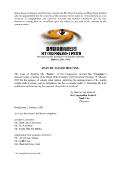
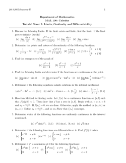
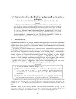
![arXiv:1501.07424v1 [math.LO] 29 Jan 2015](http://s2.esdocs.com/store/data/000457199_1-c519b33964b71d2972f4fe1f35ca3766-250x500.png)
© Copyright 2026