1. No category

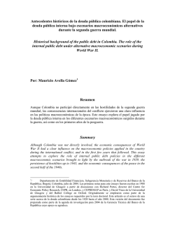
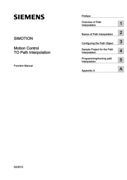
Science Journal of Applied Mathematics and Statistics
2015; 3(1): 6-13
Published online January 30, 2015 (http://www.sciencepublishinggroup.com/j/sjams)
doi: 10.11648/j.sjams.20150301.12
ISSN: 2376-9491 (Print); ISSN: 2376-9513 (Online)
A power law extrapolation – interpolation method for IBNR
claims reserving
Werner Hürlimann
Swiss Mathematical Society, Fribourg, Switzerland
Email address:
[email protected]
To cite this article:
Werner Hürlimann. A Power Law Extrapolation – Interpolation Method for IBNR Claims Reserving. Science Journal of Applied
Mathematics and Statistics. Vol. 3, No. 1, 2015, pp. 6-13. doi: 10.11648/j.sjams.20150301.12
Abstract: To calculate claims reserves more frequently than the usual yearly periods for which ultimate loss development
factors are available, it is necessary to perform an extrapolation prior to the time marking the end of the first development year
and an interpolation for each successive development year. A simple power law extrapolation – interpolation method is
developed and illustrated for monthly and quarterly sub-periods.
Keywords: Claims Reserving, IBNR Reserve, Loss Development Factors, Interpolation, Extrapolation, Power Law
1. Introduction
Claims reserves are usually the largest single item on an
insurance company’s balance sheet. Very often reserve
fluctuations significantly affect the company’s solvency
requirements and overall financial position. Any mismatch of
reserves has a direct impact on net asset values. Moreover,
capital adequacy and reserving adequacy are essentially two
sides of the same coin. An insurer whose claims reserves are
more than adequate does not need to maintain as much
capital as an insurer whose reserves are less than adequate.
Setting claims reserves accurately is a gigantic task,
especially for a complex multi-line insurer. Reserving has a
great impact on virtually everything an insurance company
does, from setting prices to establishing solvency margins.
Therefore, with the introduction of Solvency II and the new
accounting standards for insurance IFRS 4, reserving best
practices are more and more important.
By nature, claims reserves are uncertain. Essentially, they
are estimates of how much the company will have to pay out
in the future on incurred claims, whether or not they have
been reported. In simple terms, claims reserves consist of
three key elements:
Case estimates or case reserves are amounts for claims
that have been notified to the company but have not yet
been fully settled.
Incurred but not enough reported (IBNER) are
allowances for any inadequacies in case reserves.
Incurred but not reported (IBNR) are estimated amounts
for claims that have not yet been notified to the company.
Companies seldom distinguish between IBNR and IBNER,
instead combining them into a single item, called here simply
IBNR reserve. In the following, reported claims means the
sum of the actual paid claims and the case reserves.
The present note is organized as follows. Section 2 recalls
how IBNR reserves are calculated using the standard Chain
Ladder method. To report IBNR reserves more frequently
than the usual yearly periods, it is necessary to perform an
extrapolation prior to the end of the first year and an
interpolation for each successive development year. A simple
power law method is developed and illustrated for monthly
and quarterly sub-periods in Section 3.
2. Calculation of IBNR Reserves
In practice, the calculation of IBNR reserves involves an
actuary, either at the initial stage or as part of the audit process.
IBNR claims reserving can be described as “squaring the
triangle”, that is making use of historic information on the
development of paid or reported claims to make estimates
about their future development (e.g. Boulter and Grubbs [1],
Subotzky and Mazur [23]). For example, at the end of 2014, a
company that has been writing a certain class of business since
2005 has 10 annual development points for claims on its 2005
book of business, nine development points for 2006 and one
for 2014. A loss triangle can be created with either the reported
claims or the paid claims in form of a partially completed table.
The rows represent the accident years in which claims
incurred and the columns represent the development periods.
Science Journal of Applied Mathematics and Statistics 2015; 3(1): 6-13
Table 1 below is an example of loss triangle. This triangle will
form the upper left part of a square (hence the expression,
squaring the triangle) and the information in the triangle can
be used to fill in the lower right part of the square, which,
together with assumptions about the length of the
development tail (accident years going beyond 2003), will
give an estimate of the ultimate incurred claims. The
difference between the estimated ultimate claims and the
claims paid to date is the claims reserve, and the difference
between the claims reserve and the outstanding case reserves
for reported claims is the IBNR reserve.
The topic of claims reserving is well established within
actuarial mathematics. Among recent work, one finds a
handbook by Radtke and Schmidt [14], an extensive
bibliography by Schmidt [21], and Ph.D. theses by Salzmann
[17] and Happ [5].
The most commonly used IBNR reserving techniques are
the Chain Ladder and the Bornhuetter-Ferguson methods or
an optimal combination of them called Credible IBNR method
(e.g. Mack [11], Hürlimann [9], Gigante et al. [4]). The
methods are deterministic in that they give a point estimate of
ultimate claims rather than a range of estimates. Other
reserving methods, such as Bootstrapping or the Gamma
IBNR method in Hürlimann [8], are stochastic in that they use
runoff triangles to arrive at a distribution of the ultimate
claims (see also Wüthrich and Merz [24], Huang and Wu [6]).
The statistical estimation of loss development factors in Table
7
2 is based on the data of Table 1 and uses for simplicity the
Chain Ladder method.
In the Chain Ladder method, historical data is examined to
estimate loss development factors (LDF) or ratios for each
development period. The factors are cumulated and applied to
the latest observed numbers (here paid claims) to estimate the
ultimate incurred claims. The underlying assumption is that
for each year of exposure, a certain percentage of the ultimate
claims will have emerged at the end of each development year,
and these percentages are consistent across years. So, for
example, in Table 1, we can estimate the likely development
of 2003 after five years by reference to the actual development
of 1994 at 1999, 1995 at 2000, and so on.
For the mathematical specification, consider now a given
accident year of a line of business over a development period
( 0,T ] in units of years. The ultimate LDF of the yearly
( t − 1, t ] , t = 1, 2,..., T ,
exposure period
of the considered
accident year is denoted by Ft (blue line in Table 2 with
T=10). The further notations are as follows:
St : aggregate paid claims for the period ( 0, t ]
OSt : outstanding case reserves for the period ( t , T ]
IBNRt : IBNR reserve for the period ( t , T ]
By definition one has the identity:
IBNRt = ( Ft − 1) ⋅ St − OSt .
(1)
Table 1. Loss Triangle of Paid Claims ("A.M. Best" 2004 table for Private Passenger Auto Liability).
Accident
Year
1994
1995
1996
1997
1998
1999
2000
2001
2002
2003
Development Period in Months
12
24
36
16'883'850 31'182'837 37'401'111
17'518'883 31'787'614 38'274'471
18'137'677 32'509'210 39'097'072
18'449'658 32'776'770 39'487'465
18'710'148 33'568'205 40'461'509
20'553'769 36'347'062 43'531'162
22'247'399 39'116'657
46'564'786
23'082'370 40'371'884 48'011'274
24'245'392 42'085'537
24'146'487
48
40'812'822
41'833'477
42'817'313
43'255'912
44'316'727
47'472'983
50'712'030
60
42'565'347
43'692'705
44'826'451
45'264'843
46'334'427
49'515'412
72
43'422'022
44'581'536
45'792'256
46'189'365
47'208'966
84
43'832'148
45'021'089
46'264'482
46'511'626
96
44'029'002
45'233'182
46'470'822
108
44'120'908
45'338'083
120
44'172'759
Table 2. Loss Development Factors according to the Chain Ladder method.
Period in Months
Chain-ladder factors
Ultimate LDF
Percent Unpaid Claims
Percent Paid Claims
12-24
1.77805
2.52532
60.40%
39.60%
24-36
1.19869
1.42027
29.59%
30.81%
36-48
1.09270
1.18485
15.60%
13.99%
48-60
1.04487
1.08433
7.78%
7.82%
3. Extrapolation – Interpolation of
Ultimate LDF Patterns
To report IBNR reserves more frequently than the usual
yearly periods for which ultimate LDF patterns are available,
it is necessary to perform an extrapolation prior to time t = 1
marking the end of the first year and an interpolation for each
successive development year between time t − 1 and time t .
Different and more complex methods of extrapolation –
60-72
1.02025
1.03776
3.64%
4.14%
72-84
1.00914
1.01716
1.69%
1.95%
84-96
1.00455
1.00795
0.79%
0.90%
96-108
1.00220
1.00338
0.34%
0.45%
108-120
1.00118
1.00118
0.12%
0.22%
120-ult.
1.00000
1.00000
0.00%
0.12%
interpolation have been developed earlier in Sherman [22] and
Robbin and Homer [16].
For simplicity, let us focus on monthly and quarterly
sub-periods, but the method is valid for sub-periods of
arbitrary lengths. We assume that the revealed paid claims in
each sub-period of a development year behave proportionally
to a power law depending on the elapsed number of
sub-periods as follows. Let the amounts of claims paid in the
k -th sub-period of the development year ( t − 1, t ] equal
k α ⋅ ct(−α1, m ) respectively k α ⋅ ct(−α1, q ) , where ct(−α1, m ) and ct(−α1, q )
8
Werner Hürlimann:
A Power Law Extrapolation – Interpolation Method for IBNR Claims Reserving
denote appropriate increment constants for the ultimate
monthly respectively quarterly LDF patterns and α ∈ [ 0,1] .
The extreme case α = 0 refers to constant revealed paid
claims in each sub-period and the extreme case α = 1 to a
linear increase in the elapsed number of sub-periods. The
Figures 1 and 2 yield a picture of this power law method. On
the horizontal axis one finds the elapsed time and on the
vertical axis the percentage of paid claims in a given
development year.
The percentage of paid claims within a development year is
highest (smallest) for α = 0 ( α = 1 ). Other choices of the
power law exponent α ∈ [ 0,1] lie between these extremes.
A mathematical analysis yields the following formulas
U ( t − 1) − U ( t )
ct(−α1, m ) =
12
∑k
, t = 1, 2,..., T
(3)
k =1
Ft (−α1,1, m ) =
(α , m )
t −1, k
F
(α , m )
t −1
c
1
,
+ 1 − U ( t − 1)
1
= α (α , m )
, k = 2,...,12
k ⋅ ct −1 + 1 Ft (−α1,,km−)1
ct(−α1, q ) =
Monthly Power Law Pattern
U ( t − 1) − U ( t )
4
, t = 1, 2,..., T
∑ kα
(4)
(5)
k =1
100.0%
Percentage Paid Claims
α
80.0%
Ft (−α1,1, q ) =
constant
60.0%
square-root
40.0%
linear
(α , q )
t −1, k
F
20.0%
(α , q )
t −1
c
1
,
+ 1 − U ( t − 1)
1
= α (α , q )
, k = 2,3, 4
k ⋅ ct −1 + 1 Ft (−α1,,kq−) 1
(6)
0.0%
0
3
6
9
12
A verification shows that at the extrapolating respectively
interpolating times the formulas are consistent with the given
ultimate yearly LDF pattern such that
Elapsed Months
Figure 1. Monthly power-law extrapolation - interpolation pattern.
,m)
,q )
Ft (−α1,12
= Ft (−α1,12
= Ft , t = 1, 2,..., T .
Quarterly Power Law Pattern
Percentage Paid Claims
100.0%
80.0%
constant
60.0%
square-root
40.0%
In practice one is also interested in the following quantities,
where the symbol • stands for monthly (m) or quarterly
(q) :
U t(−α1,,•k)
linear
20.0%
(7)
: proportion of unpaid claims at the end of the
k -th sub-period of the development year ( t − 1, t ]
0.0%
0
1
2
3
4
Pt (−α1,,k•)
Elapsed Months
sub-period of the development year ( t − 1, t ]
Figure 2. Quarterly power-law extrapolation - interpolation pattern.
The obtained ultimate monthly and quarterly LDF patterns
after extrapolation and interpolation are elements of matrices
denoted by
Ft (−α1,,km ) : ultimate monthly LDF pattern for the k -th month
of the development period ( t − 1, t ] , t = 1, 2,..., T , k = 1, 2,...,12
Ft (−α1,,kq ) :
ultimate quarterly LDF pattern for the k -th
quarter of the development period ( t − 1, t ] , t = 1, 2,..., T , k = 1, 2,3, 4
To describe the obtained LDF patterns we will need the
following quantities:
U ( t − 1) : proportion of unpaid claims at time t − 1 for the
development period ( t − 1, t ] , t = 1, 2,..., T
By definition of the ultimate yearly LDF pattern one has
1
U ( 0 ) = 1, U ( t − 1) = 1 − , t = 2,..., T .
Ft
: proportion of paid claims during the k -th
(2)
APt (−α1,,k•) : proportion of aggregate paid claims at the end of
the k -th sub-period of the development year ( t − 1, t ]
These quantities are obtained using the following formulas:
U t(−α1,,•k) = 1 −
U
(α , • )
0,0
1
(α , • )
t −1, k
F
,
= U ( 0 ) = 1, U
(8)
(α , • )
t ,0
= U ( t − 1)
Pt (−α1,,k•) = U t(−α1,,•k)−1 − U t(−α1,,•k)
APt (−α1,,k• ) = APt (−α1,,k•)−1 + Pt (−α1,,k• ) ,
(α ,• )
AP0,0
= 0,
,•)
APt (,0α ,• ) = APt (−α1,12
(9)
(10)
To illustrate, we have calculated the ultimate monthly and
quarterly LDF patterns for the given ultimate yearly LDF
pattern of Table 2 according to the above power law method
Science Journal of Applied Mathematics and Statistics 2015; 3(1): 6-13
for the linear case α = 1 (Tables 3 and 4), the constant case
α = 0 (Tables 5 and 6) and the square root case α = 12
(Tables 7 and 8).
For comparison, percentages of unpaid claims in the
sub-periods of the different development years have also been
calculated for the linear case α = 1 (Tables 9 and 10), the
constant case α = 0 (Tables 11 and 12) and the square root
case α = 12 (Tables 13 and 14).
In the Tables 3 to 8 differences in numerical values of the
various LDF patterns are observed for all calendar years.
These are quite accentuated in the first year of development,
which requires an extrapolation method. For the monthly
LDF’s they vary in the first month from 196.98 (linear case)
and 73.86 (square root case) to 30.30 (constant case). The
quarterly LDF’s vary in the first quarter from 25.25 (linear
case) and 15.52 (square root case) to 10.10 (constant case).
The percentages of unpaid claims (Tables 9 to 14) are less
9
sensitive. For the monthly data, they vary in the first month
from 99.5% (linear case) and 98.6% (square root case) to
96.7% (constant case). The quarterly percentages vary in the
first quarter from 96% (linear case) and 93.6% (square root
case) to 90.1% (constant case). These differences are
significant enough to have a non-negligible impact on the
reporting balance sheet of an insurance company. For example,
given 100 Mio USD of expected ultimate claims, the
maximum difference in unpaid reported claims can be as large
as 5.9 Mio for claims reported in the first quarter of the first
calendar year. Of course, the differences decrease with
increasing calendar year because claims remaining unpaid
diminish. However, in some lines of business, which can take
many years to be fully developed, important differences will
remain. To obtain a unique power law exponent α ∈ [ 0,1] an
optimal criterion must be applied. This problem, which has
not yet been investigated, is open for further investigation.
Table 3. Ultimate LDF Matrix by Year and Month (linear case).
Year
0
1
2
3
4
5
6
7
8
9
Month
1
196.975
2.500
1.417
1.183
1.084
1.037
1.017
1.008
1.003
1.001
2
65.658
2.452
1.409
1.181
1.082
1.037
1.017
1.008
1.003
1.001
3
32.829
2.383
1.399
1.176
1.081
1.036
1.016
1.008
1.003
1.001
4
19.697
2.296
1.385
1.171
1.078
1.035
1.016
1.007
1.003
1.001
5
13.132
2.197
1.368
1.164
1.075
1.034
1.015
1.007
1.003
1.001
6
9.380
2.088
1.348
1.156
1.071
1.032
1.015
1.007
1.003
1.001
7
7.035
1.974
1.326
1.147
1.067
1.030
1.014
1.006
1.003
1.001
8
5.472
1.858
1.301
1.136
1.062
1.028
1.013
1.006
1.002
1.001
9
4.377
1.743
1.274
1.125
1.057
1.026
1.012
1.005
1.002
1.000
10
3.581
1.631
1.246
1.112
1.051
1.023
1.011
1.005
1.002
1.000
11
2.984
1.523
1.216
1.099
1.045
1.020
1.009
1.004
1.002
1.000
12
2.525
1.420
1.185
1.084
1.038
1.017
1.008
1.003
1.001
1.000
Yearly
Pattern
Increment
Constants
2.525
1.420
1.185
1.084
1.038
1.017
1.008
1.003
1.001
1.000
0.508%
0.395%
0.179%
0.100%
0.053%
0.025%
0.012%
0.006%
0.003%
0.002%
Table 4. Ultimate LDF Matrix by Year and Quarter (linear case).
Quarter
1
25.253
2.343
1.393
1.174
1.079
1.036
1.016
1.007
1.003
1.001
Year
0
1
2
3
4
5
6
7
8
9
2
8.418
2.047
1.340
1.153
1.070
1.031
1.014
1.007
1.003
1.001
3
4.209
1.722
1.269
1.122
1.056
1.025
1.012
1.005
1.002
1.000
Yearly
Pattern
2.525
1.420
1.185
1.084
1.038
1.017
1.008
1.003
1.001
1.000
4
2.525
1.420
1.185
1.084
1.038
1.017
1.008
1.003
1.001
1.000
Increment
Constants
3.960%
3.081%
1.399%
0.782%
0.414%
0.195%
0.090%
0.045%
0.022%
0.012%
Table 5. Ultimate LDF Matrix by Year and Month (constant case).
Year
0
1
2
3
4
5
6
7
8
9
Month
1
30.304
2.372
1.397
1.176
1.080
1.036
1.016
1.008
1.003
1.001
2
15.152
2.235
1.375
1.167
1.076
1.034
1.016
1.007
1.003
1.001
3
10.101
2.114
1.353
1.158
1.072
1.033
1.015
1.007
1.003
1.001
4
7.576
2.005
1.332
1.149
1.068
1.031
1.014
1.006
1.003
1.001
5
6.061
1.907
1.312
1.141
1.064
1.029
1.013
1.006
1.002
1.001
6
5.051
1.818
1.292
1.132
1.061
1.027
1.013
1.006
1.002
1.001
7
4.329
1.737
1.273
1.124
1.057
1.026
1.012
1.005
1.002
1.000
8
3.788
1.663
1.254
1.116
1.053
1.024
1.011
1.005
1.002
1.000
9
3.367
1.595
1.236
1.108
1.049
1.022
1.010
1.005
1.002
1.000
10
3.030
1.532
1.219
1.100
1.045
1.021
1.009
1.004
1.002
1.000
11
2.755
1.474
1.201
1.092
1.041
1.019
1.009
1.004
1.001
1.000
12
2.525
1.420
1.185
1.084
1.038
1.017
1.008
1.003
1.001
1.000
Yearly
Pattern
Increment
Constants
2.525
1.420
1.185
1.084
1.038
1.017
1.008
1.003
1.001
1.000
3.300%
2.568%
1.166%
0.652%
0.345%
0.163%
0.075%
0.038%
0.018%
0.010%
10
Werner Hürlimann:
A Power Law Extrapolation – Interpolation Method for IBNR Claims Reserving
Table 6. Ultimate LDF Matrix by Year and Quarter (constant case).
Quarter
1
10.101
2.114
1.353
1.158
1.072
1.033
1.015
1.007
1.003
1.001
Year
0
1
2
3
4
5
6
7
8
9
2
5.051
1.818
1.292
1.132
1.061
1.027
1.013
1.006
1.002
1.001
3
3.367
1.595
1.236
1.108
1.049
1.022
1.010
1.005
1.002
1.000
4
2.525
1.420
1.185
1.084
1.038
1.017
1.008
1.003
1.001
1.000
Yearly
Pattern
Increment
Constants
2.525
1.420
1.185
1.084
1.038
1.017
1.008
1.003
1.001
1.000
9.900%
7.703%
3.497%
1.956%
1.035%
0.488%
0.225%
0.113%
0.055%
0.029%
Table 7. Ultimate LDF Matrix by Year and Month (square root case).
Year
0
1
2
3
4
5
6
7
8
9
Month
1
73.863
2.460
1.411
1.181
1.083
1.037
1.017
1.008
1.003
1.001
2
30.595
2.373
1.397
1.176
1.080
1.036
1.016
1.008
1.003
1.001
3
17.814
2.274
1.381
1.169
1.077
1.035
1.016
1.007
1.003
1.001
4
12.018
2.170
1.363
1.162
1.074
1.033
1.015
1.007
1.003
1.001
5
8.812
2.065
1.344
1.154
1.071
1.032
1.015
1.007
1.003
1.001
6
6.819
1.960
1.323
1.146
1.067
1.030
1.014
1.006
1.003
1.001
7
5.480
1.859
1.301
1.136
1.062
1.028
1.013
1.006
1.002
1.001
8
4.530
1.761
1.279
1.127
1.058
1.026
1.012
1.005
1.002
1.001
9
3.826
1.668
1.256
1.117
1.053
1.024
1.011
1.005
1.002
1.000
10
3.287
1.581
1.232
1.106
1.048
1.022
1.010
1.004
1.002
1.000
11
2.865
1.498
1.209
1.095
1.043
1.020
1.009
1.004
1.001
1.000
12
2.525
1.420
1.185
1.084
1.038
1.017
1.008
1.003
1.001
1.000
Yearly
Pattern
Increment
Constants
2.525
1.420
1.185
1.084
1.038
1.017
1.008
1.003
1.001
1.000
1.354%
1.053%
0.478%
0.267%
0.141%
0.067%
0.031%
0.015%
0.008%
0.004%
Table 8. Ultimate LDF Matrix by Year and Quarter (square root case).
Quarter
1
15.521
2.242
1.376
1.167
1.076
1.034
1.016
1.007
1.003
1.001
Year
0
1
2
3
4
5
6
7
8
9
2
6.429
1.934
1.317
1.143
1.066
1.030
1.014
1.006
1.003
1.001
3
3.743
1.656
1.252
1.115
1.052
1.024
1.011
1.005
1.002
1.000
4
2.525
1.420
1.185
1.084
1.038
1.017
1.008
1.003
1.001
1.000
Yearly
Pattern
Increment
Constants
2.525
1.420
1.185
1.084
1.038
1.017
1.008
1.003
1.001
1.000
6.443%
5.013%
2.276%
1.273%
0.673%
0.318%
0.146%
0.074%
0.036%
0.019%
Table 9. Unpaid Claims Matrix by Year and Month (linear case).
Month
1
2
3
4
5
6
7
8
9
10
11
12
Yearly
Pattern
0
99.5%
98.5%
97.0%
94.9%
92.4%
89.3%
85.8%
81.7%
77.2%
72.1%
66.5%
60.4%
60.4%
1
60.0%
59.2%
58.0%
56.5%
54.5%
52.1%
49.3%
46.2%
42.6%
38.7%
34.3%
29.6%
29.6%
2
29.4%
29.1%
28.5%
27.8%
26.9%
25.8%
24.6%
23.1%
21.5%
19.7%
17.8%
15.6%
15.6%
3
15.5%
15.3%
15.0%
14.6%
14.1%
13.5%
12.8%
12.0%
11.1%
10.1%
9.0%
7.8%
7.8%
4
7.7%
7.6%
7.5%
7.2%
7.0%
6.7%
6.3%
5.9%
5.4%
4.9%
4.3%
3.6%
3.6%
5
3.6%
3.6%
3.5%
3.4%
3.3%
3.1%
2.9%
2.7%
2.5%
2.3%
2.0%
1.7%
1.7%
6
1.7%
1.7%
1.6%
1.6%
1.5%
1.4%
1.4%
1.3%
1.2%
1.1%
0.9%
0.8%
0.8%
7
0.8%
0.8%
0.8%
0.7%
0.7%
0.7%
0.6%
0.6%
0.5%
0.5%
0.4%
0.3%
0.3%
8
0.3%
0.3%
0.3%
0.3%
0.3%
0.3%
0.3%
0.2%
0.2%
0.2%
0.2%
0.1%
0.1%
9
0.1%
0.1%
0.1%
0.1%
0.1%
0.1%
0.1%
0.1%
0.0%
0.0%
0.0%
0.0%
0.0%
Year
Science Journal of Applied Mathematics and Statistics 2015; 3(1): 6-13
11
Table 10. Unpaid Claims Matrix by Year and Quarter (linear case).
Quarter
1
96.0%
57.3%
28.2%
14.8%
7.4%
3.4%
1.6%
0.7%
0.3%
0.1%
Year
0
1
2
3
4
5
6
7
8
9
2
88.1%
51.2%
25.4%
13.3%
6.5%
3.1%
1.4%
0.7%
0.3%
0.1%
3
76.2%
41.9%
21.2%
10.9%
5.3%
2.5%
1.1%
0.5%
0.2%
0.0%
Yearly
Pattern
4
60.4%
29.6%
15.6%
7.8%
3.6%
1.7%
0.8%
0.3%
0.1%
0.0%
60.4%
29.6%
15.6%
7.8%
3.6%
1.7%
0.8%
0.3%
0.1%
0.0%
Table 11. Unpaid Claims Matrix by Year and Month (constant case).
Month
1
2
3
4
5
6
7
8
9
10
11
12
Yearly
Pattern
0
96.7%
93.4%
90.1%
86.8%
83.5%
80.2%
76.9%
73.6%
70.3%
67.0%
63.7%
60.4%
60.4%
1
57.8%
55.3%
52.7%
50.1%
47.6%
45.0%
42.4%
39.9%
37.3%
34.7%
32.2%
29.6%
29.6%
2
28.4%
27.3%
26.1%
24.9%
23.8%
22.6%
21.4%
20.3%
19.1%
17.9%
16.8%
15.6%
15.6%
3
14.9%
14.3%
13.6%
13.0%
12.3%
11.7%
11.0%
10.4%
9.7%
9.1%
8.4%
7.8%
7.8%
4
7.4%
7.1%
6.7%
6.4%
6.1%
5.7%
5.4%
5.0%
4.7%
4.3%
4.0%
3.6%
3.6%
5
3.5%
3.3%
3.2%
3.0%
2.8%
2.7%
2.5%
2.3%
2.2%
2.0%
1.8%
1.7%
1.7%
6
1.6%
1.5%
1.5%
1.4%
1.3%
1.2%
1.2%
1.1%
1.0%
0.9%
0.9%
0.8%
0.8%
7
0.8%
0.7%
0.7%
0.6%
0.6%
0.6%
0.5%
0.5%
0.5%
0.4%
0.4%
0.3%
0.3%
8
0.3%
0.3%
0.3%
0.3%
0.2%
0.2%
0.2%
0.2%
0.2%
0.2%
0.1%
0.1%
0.1%
9
0.1%
0.1%
0.1%
0.1%
0.1%
0.1%
0.0%
0.0%
0.0%
0.0%
0.0%
0.0%
0.0%
Year
Table 12. Unpaid Claims Matrix by Year and Quarter (constant case).
Quarter
1
90.1%
52.7%
26.1%
13.6%
6.7%
3.2%
1.5%
0.7%
0.3%
0.1%
Year
0
1
2
3
4
5
6
7
8
9
2
80.2%
45.0%
22.6%
11.7%
5.7%
2.7%
1.2%
0.6%
0.2%
0.1%
3
70.3%
37.3%
19.1%
9.7%
4.7%
2.2%
1.0%
0.5%
0.2%
0.0%
Yearly
Pattern
4
60.4%
29.6%
15.6%
7.8%
3.6%
1.7%
0.8%
0.3%
0.1%
0.0%
60.4%
29.6%
15.6%
7.8%
3.6%
1.7%
0.8%
0.3%
0.1%
0.0%
Table 13. Unpaid Claims Matrix by Year and Month (square root case).
Year
0
1
2
3
4
5
6
7
8
9
Month
1
98.6%
59.3%
29.1%
15.3%
7.6%
3.6%
1.7%
0.8%
0.3%
0.1%
2
96.7%
57.9%
28.4%
15.0%
7.4%
3.5%
1.6%
0.8%
0.3%
0.1%
3
94.4%
56.0%
27.6%
14.5%
7.2%
3.4%
1.6%
0.7%
0.3%
0.1%
4
91.7%
53.9%
26.7%
14.0%
6.9%
3.2%
1.5%
0.7%
0.3%
0.1%
5
88.7%
51.6%
25.6%
13.4%
6.6%
3.1%
1.4%
0.7%
0.3%
0.1%
6
85.3%
49.0%
24.4%
12.7%
6.2%
2.9%
1.4%
0.6%
0.3%
0.1%
7
81.8%
46.2%
23.1%
12.0%
5.9%
2.7%
1.3%
0.6%
0.2%
0.1%
8
77.9%
43.2%
21.8%
11.2%
5.5%
2.6%
1.2%
0.5%
0.2%
0.1%
9
73.9%
40.1%
20.4%
10.4%
5.0%
2.4%
1.1%
0.5%
0.2%
0.0%
10
69.6%
36.7%
18.8%
9.6%
4.6%
2.1%
1.0%
0.4%
0.2%
0.0%
11
65.1%
33.2%
17.3%
8.7%
4.1%
1.9%
0.9%
0.4%
0.1%
0.0%
12
60.4%
29.6%
15.6%
7.8%
3.6%
1.7%
0.8%
0.3%
0.1%
0.0%
Yearly
Pattern
60.4%
29.6%
15.6%
7.8%
3.6%
1.7%
0.8%
0.3%
0.1%
0.0%
12
Werner Hürlimann:
A Power Law Extrapolation – Interpolation Method for IBNR Claims Reserving
Table 14. Unpaid Claims Matrix by Year and Quarter (square root case).
Quarter
1
2
3
4
Yearly
Pattern
0
93.6%
84.4%
73.3%
60.4%
60.4%
1
55.4%
48.3%
39.6%
29.6%
29.6%
2
27.3%
24.1%
20.2%
15.6%
15.6%
3
14.3%
12.5%
10.3%
7.8%
7.8%
4
7.1%
6.2%
5.0%
3.6%
3.6%
5
3.3%
2.9%
2.3%
1.7%
1.7%
6
1.5%
1.3%
1.1%
0.8%
0.8%
7
0.7%
0.6%
0.5%
0.3%
0.3%
8
0.3%
0.3%
0.2%
0.1%
0.1%
9
0.1%
0.1%
0.0%
0.0%
0.0%
Year
Let us conclude with a brief account of some related claims
reserving literature and possible future developments.
Usually, claims reserving models assume independence
between different accidents years. For this reason, they fail to
model claims inflation appropriately, because claims inflation
acts on all accident years simultaneously. A model that
accounts for accident year dependence in runoff triangles has
been proposed by Salzmann and Wüthrich [18].
Predictions of claims reserves often rely on individual loss
triangles, where each triangle corresponds to a different line of
business. Since different lines of business are often dependent
it is necessary to develop models for loss triangle dependence.
Examples that use copulas are Regis [15] and de Jong [2].
To take into account solvency purposes (e.g. the Solvency II
project) it is necessary to adapt the classical claims reserving
models. Some typical developments include Merz and
Wüthrich [12], Hürlimann [7], Savelli and Clemente [19], Pira
et al. [13], Eling et al. [3], Salzmann [17] and Happ [5].
Another direction concerns the development of claims
reserving models based on multiple risk factors. Besides [7]
and [20] we would like to point out [10], where the use of
stochastic LDF’s is advocated.
The integration of the presented simple extrapolation –
interpolation method in these and other recent claims
reserving techniques and the study of its impact might be a
topic for future research.
References
[1]
A. Boulter and D. Grubbs, “Late claims in reinsurance”,
Publication
Swiss
Reinsurance
Company,
URL:
http://www.swissre.com, 2000.
[5]
S. Happ, “Stochastic claims reserving under consideration of
various different sources of information”, Dissertation,
University Hamburg.
[6]
Huang, J. and X. Wu, “Stochastic claims reserving in general
insurance: models and methodologies”, 2012 China
International Conference on Insurance and Risk Management,
Qingdao, 2012.
[7]
W. Hürlimann, “Modelling non-life insurance risk for Solvency
II in a reinsurance context”, Life & Pensions Magazine,
January issue, 35-40, 2010.
[8]
W. Hürlimann, “A Gamma IBNR claims reserving model with
dependent development periods”, Proc. 37th Internat. ASTIN
Colloquium, Orlando, 2007.
[9]
W. Hürlimann, “Credible loss ratio claims reserves – the
Benktander, Neuhaus and Mack methods revisited”, ASTIN
Bulletin 39(1), 81-100, 2009.
[10] W. Hürlimann, “Random loss development factor curves and
stochastic claims reserving”, JP Journal of Fundamental and
Applied Statistics 1(1), 49-62, 2011.
[11] T. Mack, “Credible claims reserve: the Benktander method” ,
ASTIN Bulletin 30(2), 333-347, 2000.
[12] M. Merz and M.V. Wüthrich, “Modelling the claims
development result for solvency purposes”, 38th ASTIN
Colloquium, Manchester, 2008.
[13] M. Pirra, S. Forte and M. Ialenti, “Implementing a Solvency II
internal model : Bayesian stochasting reserving and parameter
estimation”, 40th ASTIN Colloquium, Madrid, 2011.
[14] M. Radtke and K.D. Schmidt, “Handbuch zur Schadenreservierung”, 2nd ed., Verlag Versicherungswirtschaft,
Karlsruhe, 2012.
[15] L. Regis, “A Bayesian copula model for stochastic claims
reserving”, working paper no. 227, Collegio Carlo Alberto,
2011.
[2]
P. De Jong, “Modeling dependence between loss triangles”,
North American Actuarial Journal 16(1), 74-86, 2012.
[3]
M. Eling, D. Diers, M. Linde and C. Kraus, “The multi-year
non-life insurance risk”, Working papers on risk management
and insurance no. 96, Institute of Insurance Economics,
University of St. Gallen, November 2011.
[16] I. Robbin, D. Homer, “Analysis of loss development patterns
using infinitely decomposable percent of ultimate curves”,
1988 Discussion Papers on Evaluating Insurance Company
Liabilities, Casual Actuarial Society, 503-538, URL:
http://www.casact.org/pubs/dpp/dpp88/88dpp501.pdf
[4]
P. Gigante, L. Picech and L Sigalotti, “Prediction error for
credible claims reserves: an h-likelihood approach”, European
Actuarial Journal 3(2), 453-470, 2013.
[17] R. Salzmann, “Stochastic claims reserving and solvency”, Diss.
ETH no. 20406, Zürich, 2012.
Science Journal of Applied Mathematics and Statistics 2015; 3(1): 6-13
13
[18] R. Salzmann, M.V. Wüthrich, “Modeling accounting year
dependence in runoff triangles”, European Actuarial Journal
2(2), 227-242, 2012.
[22] R.E. Sherman, “Extrapolating, smoothing and interpolating
development factors”, Proceedings of the Casualty Actuarial
Society LXXI, 122-199, 1984.
[19] N. Savelli and G.P. Clemente, “Stochastic claims reserving
based on CRM for Solvency II purposes”, 40th ASTIN
Colloquium, Madrid, 2011.
[23] D. Subotzuky and J. Mazur, “How do you square the triangle”,
Reinsurance Magazine, Sept. 2006.
[20] M. Schiegl, “A three dimensional stochastic model for claim
reserving”, preprint, arXiv: 1009.4146 [q-fin.RM], 2010.
[21] K.D. Schmidt, “A bibliography on loss reserving”, Technische
Universität Dresden, update November 17, 2013.
[24] M.V. Wüthrich and M. Merz, Stochastic Claims Reserving
Methods in Insurance, J. Wiley, New York, 2008.