1. Art and Diseño

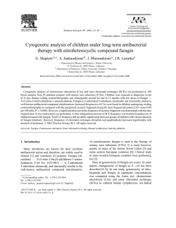
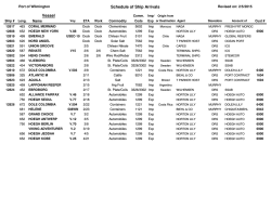
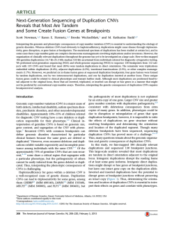
Expert Systems with Applications 36 (2009) 11925–11933
Contents lists available at ScienceDirect
Expert Systems with Applications
journal homepage: www.elsevier.com/locate/eswa
A GA-Tabu algorithm for scheduling in-line steppers in low-yield scenarios
Chie-Wun Chiou, Muh-Cherng Wu *
Department of Industrial Engineering and Management, National Chiao Tung University, 1001, Dah-Shei Road, Hsin-Chu 300, Taiwan, ROC
a r t i c l e
i n f o
Keywords:
Scheduling
Semiconductor
Flow shop
Port capacity constraints
Meta-heuristic algorithm
Genetic algorithm
Tabu search
a b s t r a c t
This paper presents a scheduling algorithm for an in-line stepper in low-yield scenarios, which mostly
appear in cases when new process/production is introduced. An in-line stepper is a bottleneck machine
in a semiconductor fab. Its interior comprises a sequence of chambers, while its exterior is a dock
equipped with several ports. The transportation unit for entry of each port is a job (a group of wafers),
while that for each chamber is a piece of wafer. This transportation incompatibility may lead to a capacity-loss, in particular in low-yield scenarios. Such a capacity-loss could be alleviated by effective scheduling. The proposed scheduling algorithm, called GA-Tabu, is a combination of a genetic algorithm (GA)
and a tabu search technique. Numerical experiments indicate that the GA-Tabu algorithm outperforms
seven benchmark ones. In particular, the GA-Tabu algorithm outperforms a prior GA both in solution
quality and computation efforts.
Ó 2009 Elsevier Ltd. All rights reserved.
1. Introduction
In semiconductor manufacturing, steppers are the most expensive machine and are usually the bottleneck of a wafer fab. Their
utilization would significantly affect the throughput of a fab. One
way to effectively utilize a stepper is by appropriately scheduling
the jobs waiting before it. Scheduling for steppers is thus an important research issue.
Much literature on stepper scheduling has been published. In
terms of problem characteristics, they vary in the inclusion of different constraints imposed on steppers—for example, mask setup
(Chern & Liu, 2003; Duwayri, Mollaghasemi, Nazzal, & Rabadi,
2006), machine dedication (Wu, Huang, Chang, & Yang, 2006;
Wu, Chiou, & Chen, 2007; Wu, Jiang, & Chang, 2008), rework
(Sha, Hsu, Che, & Chen, 2006), and cluster tool configuration (Morrison & Martin, 2007). In terms of solution methodology, four types
were mostly used: dispatching rules (Dabbas & Fowler, 2003; Ying
& Lin, 2009), artificial intelligence (Wu & Chang, 2007, 2008) mathematical programming (Chung & Hsieh, 2008), and meta-heuristic
algorithms (Chiang & Fu, 2008).
Significant milestones on stepper scheduling have been established by prior studies. However, most of them implicitly made a
high-yield assumption. That is, the production yield is quite high
so that each wafer job is a full lot (i.e., carrying 25 wafers). However, in the stage of new product/process introduction, low-yield
is quite common. Many small lots (i.e., carrying less than 25 wafers)
may appear.
* Corresponding author. Tel.: +886 3 5731 913; fax: +886 3 5720 610.
E-mail address: [email protected] (M.-C. Wu).
0957-4174/$ - see front matter Ó 2009 Elsevier Ltd. All rights reserved.
doi:10.1016/j.eswa.2009.03.064
A recent study (Wu & Chiou, 2009) indicated that an in-line stepper, a relatively advanced version of stepper, may loss capacity in a
low-yield scenario. Such a capacity-loss would not appear in a highyield scenario and has been rarely noticed. They proposed a genetic
algorithm (GA) for scheduling an in-line stepper. Their experiment
results indicated that the GA outperforms four heuristic scheduling
rules widely used in practice.
This paper aims to develop a more effective scheduling algorithm for an in-line stepper. The algorithm we proposed is called
GA-Tabu, which is a combination of a GA and a tabu search technique. Experiment results indicated that the GA-Tabu outperform
seven other meta-heuristic methods, including the GA by Wu
and Chiou (2009).
The remainder of this paper is organized as follows. Section 2
introduces the operational mechanism of an in-line stepper. Section 3 describes how to compute the makespan of a job sequence.
Section 4 presents the GA-Tabu algorithm. Experiment results are
reported in Section 5. Concluding remarks are in the last section.
2. Operational mechanism of an in-line stepper
An in-line stepper is a machine, whose interior comprises a
group of chambers, each of which can process one wafer at a time.
Its exterior is equipped with a dock for job entry/departure (Fig. 1).
Jobs are moved from a neighboring WIP buffer to the dock. The
transportation unit between the WIP buffer and the dock is a job
(a container carrying 1–25 wafers), but that between the dock
and the in-line stepper is a piece of wafer. A transportation incompatibility thus exists between the dock and the in-line stepper.
As shown in Fig. 2, an in-line stepper is composed of two modules—a track and an aligner (Quirk, 2001; Xiao, 2001). Each module
11926
C.-W. Chiou, M.-C. Wu / Expert Systems with Applications 36 (2009) 11925–11933
WIP
Dock
Buffers
Area
Track
Aligner
and looked for an available chamber that can finish the wafer at
the earliest time. We first give notation and proceed to the makespan evaluation procedure, where a group of functionally identical
chambers is called a stage.
3.1. Notation
In-line stepper
Fig. 1. Production system of stepper.
involves various types of chambers. Each type of chamber may be
more than one in numbers. In the aligner module, a mask setup
time is needed at the exposure chamber, while a wafer from a different job enters the chamber.
The dock of an in-line stepper typically involves four ports. Each
port could accommodate only one job container. A job container on
the dock must stay at the port until all its wafers have completed
processing. This implies that any other jobs cannot access the inline stepper while all the ports have been occupied. As a result, a
capacity-loss may appear in a low-yield scenario, due to the limit
of port number.
An example of such a capacity-loss is given below. Consider an
in-line stepper that has four ports and 22 chambers. Four jobs (A,
B, C, and D) are now on the dock. Job A contains 25 wafers while
jobs B, C, D in total carry only 16 wafers. Suppose the processing
sequence isA, B, C and D. When Job A’s last wafer leaves the stepper
for the dock, the 16 wafers of jobs B, C, and D would occupy the last
16 chambers of the stepper. This results in a capacity-loss—the first
six (22–16) chambers have no new wafers to host. Such a capacityloss would not occur in a high-yield scenario, in which the total
number of wafers in B, C, and D is usually more than 22.
j
k
i
l
a
q
n
M
mi
piljk
p
p(j)
w(j)
tu
td
Si,l,p(j),k
index of job
index of wafer
index of stage
index of chamber
index of the exposure chamber
total number of ports in the dock
total number of jobs to be processed by the in-line stepper
total numbers of stages in the in-line stepper
total number of chambers at stage i
processing time required for chamber l at stage i to process
wafer k in job j
a job sequence for n jobs, p = [p(1), . . ., p(n)]
the job in the jth position of a sequence p
total number of wafers in job j
transportation time for uploading a job to the dock
transportation time for downloading a job from the dock
setup time required for chamber l in stage i to process waif i–a or k–1; then Si;l;pðjÞ;k ¼ 0;
fer k in job p(j)
otherwise; Si;l;pðjÞ;k ¼ dpðjÞ;pðj1Þ
dp(j),p(j1) setup time required for the exposure chamber to switch
production from job p(j 1)to job p(j); dp(j),p(j1) = s0 if
p(j 1) and p(j) use different masks, and dp(j),p(j1) = 0,
otherwise
the time epoch when chamber l in stage i just turns to be
Ai,l,t
available. That is, while the chamber (i, l) is free at t, Ai,l,t is
the last wafer-completion-epoch before t; while the chamber (i, l) is in operation at t, Ai,l,t is the first wafer-completion-time after t
the completion-time of wafer k in job p(j) at stage i
Ci,p(j),k
Cmax(p) makespan of job sequence p
3. Makespan evaluation for job sequences
3.2. Evaluation procedure
A method, adapted from Ruiz and Maroto (2006), is presented
for evaluating the makespan of a job sequence. In the evaluation,
we virtually sent each wafer in sequence into the in-line stepper
The makespan evaluation procedure is governed by the following four equations:
Fig. 2. Configuration of an in-line stepper. (a) Vapor prime: v1–v2, (b) cooling: hc1–hc4, (c) Coater: k1–k2, (d) softbake: s1–s2, (e) cooling: sc1–sc2, (f) buffer b1–b3, (g) cooling:
pc1–pc2, (h) develop: d1–d2, (i) hard bake: h1–h2.
C.-W. Chiou, M.-C. Wu / Expert Systems with Applications 36 (2009) 11925–11933
C i;pðjÞ;k ¼ min fmaxfAi;l;t þ Si;l;pðjÞ;k ; C i1;pðjÞ;k g þ pi;l;pðjÞ;k g
16l6mi
where t ¼ C i1;pðjÞ;k
for 1 6 i 6 M
C Mþ1;pðjÞ;wðpðjÞÞ ¼ C M;pðjÞ;wðpðjÞÞ þ td
C Mþ1;pðjÞ;wðpðjÞÞ þ t u ¼ C 0;pðjþqÞ;1
C max ðpÞ ¼ C Mþ1;pðnÞ;wðpðnÞÞ
ð1Þ
ð2Þ
for 1 6 j 6 n q
ð3Þ
ð4Þ
Eq. (1) expresses the completion-time of a particular wafer at
each stage i. The term Ai,l,t + Si,l,p(j),k denotes the time epoch when
chamber l at stage i is ready for processing wafer k in job p(j),
and the term Ci1,p(j),k denotes the time epoch when the wafer is
available to be processed at the chamber.
Eq. (2) describes the completion-time of job p(j) at stage M + 1,
where we assume that a waiting-for-process wafer in the port is at
stage 0; and a finished wafer in the port is at stage M + 1.
Eq. (3) expresses the job arrival/departure relationships for the
dock. The equation indicates that job p(j + q) in the WIP buffer can
be transported to the dock only when job p(j) in the dock has been
moved away. Eq. (4) computes the makespan Cmax(p).
4. Algorithm
An algorithm called GA-Tabu, a combination of a GA (Holland,
1975) with a tabu search technique, is proposed to solve the in-line
stepper scheduling problem. In the algorithm, a chromosome (a job
sequence) is denoted by p = [p(1), . . ., p(n)] where p(j), called a
gene, represents the job in the jth position of sequence p. The
makespan Cmax(p) of the chromosome is called its fitness function.
We first introduce the logic flow of the GA-Tabu algorithm, and
proceed to describe each major component in the algorithm.
4.1. Logic flow
The logic flow of the proposed algorithm is described by a main
procedure named GA-Tabu, in which a sub-procedure named Tabu
will be called.
Procedure GA-Tabu
Step 1: Initialization
Set k = 0 and t = 0. Randomly select Np chromosomes to form
an initial population P(t). Identify the best chromosome p0b
in P(0).
Set po ¼ p0b /po is the currently best ever solution; k is the
tenure of po /
Set tabu_list = / /tabu_list is a queue list of size q /
Set p ¼ p0b /p is a chromosome called tabu_seed /
Step 2: Update P(t + 1) by GA
Use crossover operators to create a set N1(t) of Pcr Np new
chromosomes.
Use mutation operators to create a set N2(t) of Pm Np new
chromosomes.
Let S(t) = P(t) [ N1(t) [ N2(t). From S(t), use a selection strategy (the roulette wheel selection method by Michalewicz
(1996) to select Np chromosomes to form P(t + 1)).
Step 3: Update po based on pbest, the best chromosome in P(t + 1)
From P(t + 1), identify the best chromosome pbest
If Cmax(pbest) P Cmax(po) set k = k + 1, go to Step 4.
If Cmax(pbest) < Cmax(po), set k = 0 /while pbest is better than
po /
Set po = pbest / update po by pbest /
call Tabu(pbest, po); / further update po by tabu /
Step 4: Update po based on good chromosomes in P(t + 1) other
than pbest
If k = 20, call Tabu(pin, po), where pin is the 2nd best chromosome in P(t + 1)
11927
If k = 30, call Tabu(pin, po); pin is the 3rd chromosome in
P(t + 1)
If k = 40, call Tabu(pin, po); pin is the 4th chromosome in
P(t + 1)
Step 5: Update po and p based on the current tabu seed
If (k > 40 & mod (k, 5) = 0), call Tabu(p, po)
Step 6: Termination Check
If (k = K or t = T), then stop
Otherwise, set t = t + 1, go to Step 3.
Procedure Tabu(pin, pout)
Step 1: Create a set X of new chromosomes.
Based on pin, apply the steepest descent pairwise interchange
(SDPI) (Armour & Buffa, 1963) technique to create a set X of
new chromosomes. Each new chromosome p is created by
applying a particular interchange operation, represented by
move(p)
Step 2: Update tabu_list
From X, identify the best q chromosome p1b ; . . . ; pqb
For i = 1, q
If mov eðpib Þ R tabu_list, then
Place mov eðpib Þ in the tabu_list;
Set pout ¼ pib ;
Replace the worst chromosome in P(t + 1) by pout /
update P(t + 1) /
Go to Step 3
Endif
Endfor
Step 3: Update po and p
If Cmax(pout) < Cmax(po), set po = pout and k = 0; /update po /
If (pin = p), set p = pout; /update p /
Return.
Procedure GA-Tabu is explained below. In Step 1, we create an
initial population of chromosomes P(0) and set the initial status of
po and p, where po is the currently best ever chromosome and p
is a chromosome called tabu_seed.
In Step 2, we update P(t) by crossover operators, mutation operators and a selection strategy. Crossover and mutation operators
are used to create new chromosomes. The existing and new chromosomes are then screened by the selection strategy in order to
create P(t + 1) from P(t).
In Step 3, we intend to update po based on pbest, the best chromosome in P(t + 1). If pbest is better than po, this implies that pbest is
a good chromosome and its neighborhood could be exploited further. To do so, we call Procedure Tabu to create a new chromosome
pout from the neighborhood of pbest. Of the two chromosomes pbest
and pout, the better one if eligible is used to update po. If po is not
updated in an iteration t, its tenure k is increased by one. The tenure k indicates how many times po has outperformed pbest while
P(t) is evolving. A large k value implies that update po based on current pbest in P(t + 1) appears to be difficult to a certain extent.
Therefore, in Step 4, some good chromosomes other than pbest in
P(t + 1) are considered to update po. That is, we use the 2nd, 3rd,
and 4th best chromosomes in P(t + 1) and call Procedure Tabu to
exploit their neighborhood in order to create new chromosomes
for possibly replacing po. In essence, both Steps 3 and 4 are intended to update po through the use of P(t + 1), which evolves
based on the GA technique. While the value of k is too large (here
we set k > 40), we could infer that updating po through the use of
GA is now hard to a certain extent.
To remedy this deficiency, in Step 5, we alternatively use tabu_seed p and call Procedure Tabu to exploit its neighborhood in order to create new chromosomes for possibly replacing po. The
evolution of p is independent of the GA. Therefore, p is likely
far away from the neighborhood of the chromosomes in P(t + 1).
11928
C.-W. Chiou, M.-C. Wu / Expert Systems with Applications 36 (2009) 11925–11933
This characteristic helps the algorithm escape from a local optimal
solution obtained by the GA.
Procedure Tabu(pin, pout) is designed to create a new chromosome pout, which is one in the neighborhood of pin. One purpose
for obtaining pout is for updating po and P(t + 1). The input pin
has two possible sources: P(t + 1) or tabu_seed p. The source p
is designed to evolve through this procedure. Therefore, we additionally use pout to update p while pin = p. In summary, Procedure
Tabu has three functions: updating po, p and P(t + 1).
1
6
3
9
4
5
8
7
2
Parent 2
3
5
6
1
8
2
7
9
4
x-child-1
1
6
3
x-child-2
3
5
6
Parent 1
1
6
3
9
4
5
8
7
2
Child-2
3
5
6
1
9
4
8
7
2
3
4
5
8
7
2
1
6
8
9
4
5
3
7
2
1
6
3
9
4
5
8
7
2
1
6
3
8
5
4
9
7
2
1
6
3
9
4
5
8
7
2
1
5
8
7
6
3
9
4
2
C1 operator: Referring to Fig. 3a, one randomly selected point is
used to divide each parent into two sections (head and tail). To create an offspring (say, child-2), its head is copied from the head of
parent-2—a string (3, 5, 6) in this case. Its tail is determined by
sequentially referring to the genes of parent-1; only the gene values not in the head of child-2 are eligible to appear in the tail. This
results in a string (1, 9, 4, 8, 7, 2) as the tail of child-2.
LOX operator: Referring to Fig. 3b, each parent is randomly divided into three sections (head, middle and tail). The middle for parent-1 and parent-2 are (3, 9, 4) and (6, 1, 8) respectively. A
b. LOX (Linear order crossover)
Parent 1
Parent 2
9
Fig. 4. Mutation operators: (a) SWAP, (b) Inverse, (c) Insert.
a. C1 crossover
6
3
c. Insert
To create new chromosomes, we use four types of crossover
operators and three types of mutation operators. A crossover operator is designed to create a new pair from an existing pair, while a
mutation operator is to create a new one from an existing one. The
four types of crossover operators are C1 (one point crossover) by
Reeves (1995), LOX (linear order crossover) by Croce, Tadei, and
Volta (1995), PMX (partially mapped crossover) by Goldberg
(1989), and NABEL operator by Bac and Perov (1993). The three
types of mutation operators are Swap, Inverse, and Insert (Nearchou, 2004; Wang & Zheng, 2003; Zhang, Wang, & Zheng, 2006).
The four crossover operators are explained below, where parent-1 and parent-2 denote parent chromosomes while child-1 and
child-2 denote the created ones.
1
6
b. Inverse
4.2. Crossover and mutation operators
Child 1
1
a. SWAP
1
6
3
9
4
5
8
7
2
Parent
2
3
5
6
1
8
2
7
9
4
Two cutting sites of the parents are chosen randomly 2,5
3
5
Parent
1
5
6
8
1
2
8
7
2
9
7
x-child-1
H
H
3
9
4
5
H
7
2
x-child-2
H
5
6
1
8
2
7
H
H
y-child-1
3
9
H
H
H
4
5
7
2
y-child-2
5
2
H
H
H
1
8
2
7
Child 1
3
9
6
1
8
4
5
7
2
Child 2
5
6
3
9
4
1
8
2
7
4
9
4
c. PMX (Partially Mapped Crossover)
Parent 1
1
6
3
9
4
5
8
7
2
Parent 2
3
5
6
1
8
2
7
9
4
d. NABEL operator
Parent 1
1
6
3
9
4
5
8
7
2
Parent 2
3
5
6
1
8
2
7
9
4
Parent 1
1
6
3
9
4
5
8
7
2
Parent 2
3
5
6
1
8
2
7
9
4
Child 1
3
4
5
1
7
6
8
2
9
Two cutting sites of the parents are chosen randomly 3,7
x-child-1
1
8
2
7
x-child-2
9
4
5
8
Parent 1
1
6
3
9
4
5
8
7
2
child-1
9
6
3
1
8
2
7
4
5
Child 2
3
1
6
9
4
5
8
2
7
Parent 2
3
5
6
1
8
2
7
9
4
Fig. 3. Crossover operators: (a) C1, (b) PMX, (c) LOX, (d) NABEL.
11929
C.-W. Chiou, M.-C. Wu / Expert Systems with Applications 36 (2009) 11925–11933
chromosome x-child-1 is created by two steps. First, its middle is
copied from the middle of parent-1. Second, its genes values that
appear in the middle of parent-2 are replaced by ‘‘H”. This yields
x-child-1 = (H, H, 3, 9, 4, 5, H, 7, 2). We then manipulate x-child-1
by moving ‘‘H” to the middle and yield a chromosome y-child1 = (3, 9, H, H, H, 4, 5, 7, 2). Finally, the middle of y-child-1 is replaced by that of parent-2; this yield child-1 = (3, 9, 6, 1, 8, 4, 5, 7, 2).
PMX operator: Referring to Fig. 3c, each parent is randomly divided into three sections (head, middle, and tail). A new offspring
(e.g., child-1) is created by the following procedure. The middle of
child-1 is created by referring to that of parent-2, which is a string
(1, 8, 2, 7). Both the head and tail of child-1 are created by referring
to parent-1. If the gene values in the head/tail sections of parent-1
do not appear in child-1, we copy them in the exact positions of
child-1 (e.g., gene values 6 and 3). Finally, for those vacant genes
in child-1, we place their values by sequentially referring to the
unassigned genes in parent-1. This yields child-1 = (9, 6, 3, 1, 8, 2,
7, 4, 5).
NABEL operator: Suppose the two parent chromosomes are
pp1 = [pp1(1), . . ., pp1(n)] and pp2 = [pp2(1), . . ., pp2(n)]; and the two
children chromosomes to be created are pc1 = [pc1(1), . . ., pc1(n)]
and pc2 = [pc2(1), . . ., pc2(n)]. Referring to Fig. 3d, the NABEL operator is designed to set pc1(i) = pp1(pp2(i)) and pc2(i) = pp2(pp1(i)). For
example, pp2(2) = 5 and pp1(pp2(2)) = 4, and we can obtain
pc1(2) = pp1(pp2(2)) = 4.
The three mutation operators are explained below, where pa
denotes the parent chromosome while pb denotes the child one.
Swap operator: Referring to Fig. 4a, we randomly choose two
distinct genes in pa, and then swap their gene values to create pb.
Inverse operator: Referring to Fig. 4b, we randomly select two
cut-off points in pa to divide it into three sections. Represent pa =
{pa1, pa2, pa3} and pa2 = [pa2(1), . . ., pa2(m)]. The inverse operator is
designed to create a new chromosome pb = {pa1, pb2, pa3} where
pb2(i) = pa2(m + 1 i).
Insert operator: Referring to Fig. 4c, we randomly select an insert point and a segment of genes in pa. This would divide pa into
four sections pa = {pa1 j pa2, pa3 ,pa4} which denote that the insert
point is between pa1 and pa2, and the selected segment is pa3. To
create a new chromosome, the insert operator moves the selected
segment to the insert point position. This would yield a new chromosome pb = {pa1, pa3 j pa2,pa4}.
bu_list. This implies that the tabu_list is designed to record ‘‘good”
and ‘‘new” moves. Such a design is to avoid a cyclic creation of the
same chromosome. This would keep po and p away from being
trapped into a local optima.
5. Numerical experiments
By numerical experiments, we justify the effectiveness of the
proposed GA-Tabu algorithm. The in-line stepper is assumed to
have four ports, 14 stages and 21 chambers. The operation time
at each chamber i follows a uniform distribution [ai, bi] (Table 1).
A mask setup is always required for the exposure chamber while
it turns to process a new job’s wafer, and the mask change time
is a constant (1.0 min). Parameters in the GA-Tabu are set as follows: P = 100, Pcr = 0.8, Pmu = 0.2, q = 7, K = 3000, T = 100,000.
5.1. Test cases
To model the process yield in experiments, we use a truncated
binomial distribution (TBD). The TBD implies that the job size is governed by a binomial distribution; however, the jobs carrying no wafer are moved away from the fab.
We use (N, Y) to represent a test case, where N represents the
number of jobs and Y represents the average yield. In our experiments, N involves five options ranging from 20 to 100 jobs while
Y involves 10 options ranging from 15% to 90% (Table 2–6). That
is, each algorithm has 50 test cases, and each test case is justified
by 15 replicates.
5.2. Benchmark algorithms
For each test case, we compare the GA-Tabu with seven other
algorithms: optimum heuristic rule (OHR), simulated annealing
(SA) by Osman and Potts (1989), GA by Wu and Chiou (in press),
tabu search (TS) by Widmer and Hertz (1989), two ant colony algorithms (ACO) by Rajendran and Ziegler (2004), and particle swarm
optimization (PSO) by Liaoa, Tseng, and Luarnb (2007). The OHR
algorithm denotes taking the best result out of three heuristic
scheduling rules: SPT (shortest job processing time), LPT (longest
job processing time), and NEH (Nawaz, Enscore, & Ham, 1983).
The two ACOs are respectively called MMAX and PACO.
For each algorithm in each test case, the average makespan of
the 15 replicates is taken as the performance. Define the average
makespan of each algorithm as follows: CGA-tabu for the GA-Tabu,
COHR for the OHR, CSA for the SA, CGA for the GA, CTS for the TS, CMMAX
for the MMAX, CPACO for the PACO, and CPSO for the PSO. The computation time for each algorithm is defined accordingly; for example, that for the GA-Tabu is defined as tGA-tabu.
4.3. Procedure Tabu
In Step 1 of Procedure Tabu, a set X of new chromosomes is created by the SDPI technique. Given a chromosome pin, the technique
creates a new one by choosing a pair of genes from pin and interchanges their values. With n genes inpin, X would include C(n, 2)
new chromosomes. For a new chromosome p = [p(1), . . ., p(i) . . .,
p(j), . . ., p(n)], where p(i)and p(j) are the two genes that are interchanged. Then, its interchange operation move(p) is represented
{p(i), p(j)}.
In Step 2 of the procedure, out of X, only the best possible chromosome created by a ‘‘new” move is eligible for updating po, p,
and P(t + 1). Herein, a ‘‘new” move is one, currently not in the ta-
5.3. Experiment results
To compare the solution quality between the GA-Tabu and a
benchmark algorithm (say, x), a performance metric is so defined:
cx = (Cx CGA_Tabu)/CGA_Tabu. A positive cx indicates that the GA-Tabu
Table 1
Process times of in-line stepper chambers.
Process
sequence
WIP
buffers to
dock area
Dock
area to
track
HMDS
Cooling
Coater
Softbake
Cooling
Aligner
Wafer
edge
exposure
PEB
Cooling
Develop
Hard
bake
High
cooling
Chamber
number
Process time
(min)
1
1
2
2
2
2
2
1
1
2
2
2
2
1
2.5
0.1
1.2
1.2
1.2
[1.2, 2.8]
1
[0.75, 1.65]
1
[1.2, 2.8]
1
[1.2, 2.8]
[1.2, 2.8]
0.5
11930
Table 2
Makespan comparison at different binomial yield scenarios for job 20.
Jobs
20
GA_Tabu
OHR
GA
SA
Tabu
MMAX
PACO
PSO
CGA-tabu
(min)
tGA-tabu
(s)
Random
(min)
SPT
(min)
LPT
(min)
NEH
(min)
CB
(min)
CGA
(min)
cGA
tGA
(s)
CSA
(min)
cSA
Ctabu
(min)
Cmax
(min)
Cpaco
(min)
(%)
tpaco
(s)
CPSO
(min)
cPSO
(%)
tmax
(s)
cpaco
(%)
ttabu
(s)
cmax
(%)
tSA
(s)
ctabu
(%)
(%)
Tpso
(s)
90
80
70
60
50
40
30
25
20
15
562.0
529.8
448.0
391.2
349.8
268.4
215.4
161.8
138.6
125.8
109
100
101
89
84
62
59
47
44
42
572.6
539.9
458.0
400.5
359.1
277.0
224.8
174.9
159.2
146.3
571.6
537.1
454.2
398.4
356.5
276.6
222.9
170.9
150.1
143.4
565.1
532.9
450.9
395.1
353.3
272.4
220.0
168.9
151.3
141.0
565.2
534.2
453.1
394.4
353.6
272.6
219.2
168.5
149.2
139.7
565.1
532.9
450.9
394.4
353.3
272.4
219.2
168.5
149.2
139.7
562.1
529.8
448.0
391.3
349.8
268.4
215.4
161.9
139.4
127.4
0.01
0.00
0.00
0.01
0.00
0.00
0.00
0.05
0.54
1.28
251
230
215
175
214
114
137
132
131
131
563.2
530.8
448.8
392.2
350.9
269.6
216.3
163.9
144.1
132.0
0.21
0.18
0.18
0.26
0.30
0.43
0.41
1.29
3.98
4.92
9
8
7
7
5
5
4
3
3
3
562.0
529.8
448.0
391.2
349.8
268.4
215.4
161.8
138.6
126.3
0.00
0.00
0.00
0.00
0.00
0.00
0.00
0.00
0.01
0.37
70.3
70.0
69.7
69.4
68.9
68.2
67.0
67.0
66.1
66.0
562.5
530.0
448.3
391.6
350.0
268.8
215.7
162.0
139.3
127.7
0.08
0.03
0.08
0.09
0.05
0.13
0.12
0.11
0.50
1.49
31
29
24
21
19
14
11
8
7
6
562.6
530.2
448.4
391.6
350.1
268.8
215.6
162.2
140.4
127.8
0.10
0.08
0.09
0.10
0.09
0.14
0.06
0.24
1.28
1.57
23
21
18
16
14
11
8
6
5
5
566.7
534.2
452.4
396.0
354.4
272.9
220.6
167.9
148.3
136.4
0.84
0.82
0.99
1.22
1.31
1.65
2.41
3.74
6.99
8.38
2
2
1
1
1
1
1
1
1
1
CSA
(min)
cSA
Cpaco
(min)
cpaco
CPSO
(min)
cPSO
(%)
tpaco
(s)
(%)
Tpso
(s)
1158.0
1001.o
901.2
775.1
685.6
526.2
405.8
351.6
292.6
261.4
1155.8
1001.4
901.8
773.9
677.9
519.4
406.0
348.9
309.8
251.7
0.01
0.04
0.06
0.03
0.02
0.05
0.05
0.09
0.05
1.78
185
160
143
122
106
81
63
54
48
34
1163.5
1008.8
909.5
781.8
685.7
526.9
413.5
358.9
313.6
273.0
0.68
0.78
0.91
1.04
1.17
1.49
1.90
2.97
1.25
10.37
7
7
6
6
6
6
5
5
5
5
Table 3
Makespan comparison at different binomial yield scenarios for job 40.
Jobs
40
GA_Tabu
OHR
GA
SA
Yield
(%)
CGA-tabu
(min)
tGA-tabu
(s)
Random
(min)
SPT
(min)
LPT
(min)
NEH
(min)
CB
(min)
CGA
(min)
cGA
(%)
tGA
(s)
90
80
70
60
50
40
30
25
20
15
1155.6
1001.0
901.3
773.7
677.8
519.2
405.9
348.6
309.7
247.3
381
333
294
276
261
182
150
150
128
104
1170.0
1015.7
914.7
787.9
691.0
531.9
419.0
367.3
332.8
290.7
1170.6
1011.9
910.7
781.5
685.7
527.2
413.8
358.8
319.7
268.2
1158.7
1004.4
905.4
778.3
681.8
523.8
411.3
356.1
319.3
267.2
1160.6
1008.0
906.8
781.4
683.1
525.7
411.9
357.3
314.4
272.9
1158.7
1004.4
905.4
778.3
681.8
523.8
411.3
356.1
314.4
267.2
1155.6
1001.0
901.3
773.7
677.8
519.2
405.9
348.6
309.7
251.4
0.00
0.00
0.00
0.00
0.00
0.00
0.01
0.02
0.00
1.65
722
635
674
553
488
359
334
419
386
649
Tabu
MMAX
Ctabu
(min)
ctabu
(%)
tSA
(s)
0.21
0.00
0.01
0.19
1.15
1.35
0.01
0.86
5.52
5.69
30
31
30
28
26
24
22
21
20
19
1155.6
1001.0
901.3
773.7
677.8
519.2
405.9
348.6
309.7
247.9
PACO
Cmax
(min)
cmax
(%)
ttabu
(s)
(%)
tmax
(s)
0.00
0.00
0.00
0.00
0.00
0.00
0.01
0.00
0.01
0.21
160
155
151
146
143
138
133
130
129
124
1155.9
1001.2
901.8
774.0
678.0
519.6
406.2
348.9
309.8
251.2
0.03
0.02
0.06
0.04
0.02
0.08
0.08
0.10
0.05
1.55
261
226
203
173
150
116
89
76
69
48
PSO
C.-W. Chiou, M.-C. Wu / Expert Systems with Applications 36 (2009) 11925–11933
Yield
(%)
Table 4
Makespan comparison at different binomial yield scenarios for job 60.
Jobs
60
GA_Tabu
OHR
GA
SA
CGA-tabu
(min)
tGA-tabu
(s)
Random
(min)
SPT
(min)
LPT
(min)
NEH
(min)
CB
(min)
CGA
(min)
cGA
90
80
70
60
50
40
30
25
20
15
1707.1
1503.7
1323.1
1192.7
960.6
794.1
566.7
472.7
417.3
367.7
961
838
792
694
517
433
324
284
281
212
1726.0
1521.8
1341.1
1210.2
977.2
811.1
586.4
502.6
462.3
454.9
1730.6
1519.5
1335.8
1201.3
967.4
801.4
578.0
486.1
445.8
400.2
1710.2
1508.0
1328.1
1197.3
964.8
798.6
575.5
482.2
444.1
399.4
1714.3
1510.8
1329.8
1199.6
967.3
800.5
577.2
489.4
452.3
397.2
1710.2
1508.0
1328.1
1197.3
964.8
798.6
575.5
482.2
444.1
397.2
1707.1
1503.7
1323.1
1192.7
960.6
794.1
566.7
472.8
419.2
370.0
Tabu
CSA
(min)
cSA
(%)
tGA
(s)
0.00
0.00
0.00
0.00
0.00
0.00
0.00
0.03
0.44
0.61
1670
1245
1549
1091
980
771
726
858
1384
1595
1710.9
1513.3
1334.5
1203.0
970.8
804.8
570.1
485.2
434.8
386.7
MMAX
Ctabu
(min)
ctabu
(%)
tSA
(s)
0.23
0.64
0.87
0.86
1.06
1.35
0.60
2.66
4.18
5.16
25
23
22
19
18
16
14
13
11
10
1707.1
1503.7
1323.1
1192.7
960.6
794.1
566.7
472.7
417.8
368.7
CSA
(min)
cSA
(%)
tSA
(s)
2288.4
2049.6
1819.6
1553.1
1344.5
1055.0
848.8
695.5
624.5
504.0
0.63
0.71
0.80
0.91
1.12
1.39
1.67
3.03
6.12
4.08
49
47
43
39
36
32
28
26
24
21
PACO
Cmax
(min)
cmax
(%)
ttabu
(s)
0.00
0.00
0.00
0.00
0.00
0.00
0.00
0.01
0.11
0.28
527
511
495
483
466
452
431
421
417
411
1707.2
1503.9
1323.1
1192.9
960.9
794.4
566.7
472.8
419.8
373.7
Ctabu
(min)
ctabu
(%)
ttabu
(s)
2274.0
2035.1
1805.3
1539.1
1329.6
1040.5
834.9
675.1
588.5
484.6
0.00
0.00
0.00
0.00
0.00
0.00
0.00
0.00
0.01
0.07
1210
1174
1139
1098
1074
1034
998
967
954
931
PSO
Cpaco
(min)
cpaco
(%)
tmax
(s)
CPSO
(min)
cPSO
(%)
tpaco
(s)
(%)
Tpso
(s)
0.00
0.02
0.00
0.02
0.04
0.05
0.01
0.04
0.60
1.62
876
773
679
612
487
401
282
240
216
162
1707.3
1503.7
1323.3
1192.8
960.8
794.3
566.9
473.1
421.1
374.5
0.01
0.00
0.02
0.00
0.02
0.03
0.04
0.10
0.90
1.83
618
542
475
427
339
278
197
166
149
112
1718.7
1514.4
1334.3
1203.6
971.5
805.5
578.9
490.9
450.0
389.8
0.68
0.71
0.85
0.92
1.14
1.44
2.15
3.86
7.82
6.00
17
17
16
16
15
15
15
15
14
14
Cmax
(min)
cmax
(%)
tmax
(s)
Cpaco
(min)
cpaco
CPSO
(min)
cPSO
(%)
tpaco
(s)
(%)
Tpso
(s)
2274.4
2035.3
1805.4
1539.3
1329.7
1040.7
834.9
675.2
589.2
491.9
0.02
0.01
0.01
0.02
0.00
0.02
0.00
0.03
0.12
1.59
2084
1857
1648
1393
1205
954
744
610
543
366
2274.2
2035.1
1805.3
1539.3
1329.8
1040.8
835.0
675.5
590.0
492.8
0.01
0.00
0.00
0.02
0.02
0.03
0.02
0.07
0.25
1.76
1474
1309
1158
978
844
660
521
426
374
253
2289.0
2049.2
1819.7
1553.1
1343.6
1054.7
8485
693.8
623.0
515.5
0.66
0.69
0.80
0.91
1.05
1.36
1.63
2.78
5.86
6.45
34
33
33
32
32
31
31
30
30
30
Table 5
Makespan comparison at different binomial yield scenarios for job 80.
Jobs
80
GA_Tabu
OHR
GA
SA
Yield
(%)
CGA-tabu
(min)
tGA-tabu
(s)
Random
(min)
SPT
(min)
LPT
(min)
NEH
(min)
CB
(min)
CGA
(min)
cGA
(%)
tGA
(s)
90
80
70
60
50
40
30
25
20
15
2274.0
2035.1
1805.3
1539.1
1329.6
1040.5
834.9
675.1
588.5
484.2
1851
1731
1659
1352
1130
864
708
601
529
392
2297.0
2056.4
1827.3
1561.2
1351.3
1061.9
855.2
703.1
639.0
727.8
2305.3
2055.0
1818.1
1547.4
1338.9
1053.1
844.0
688.1
616.3
517.1
2277.7
2038.8
1809.8
1544.4
1335.0
1050.9
841.5
684.3
614.9
517.2
2282.8
2043.7
1813.3
1547.7
1337.7
1050.0
843.5
685.3
625.6
525.1
2277.7
2038.8
1809.8
1544.4
1335.0
1050.0
841.5
684.3
614.9
517.1
2274.0
2035.1
1805.3
1539.1
1329.6
1040.5
834.9
675.1
588.9
487.1
0.00
0.00
0.00
0.00
0.00
0.00
0.00
0.01
0.07
0.59
2502
2722
2053
1767
1726
1109
1262
1315
1997
2126
Tabu
MMAX
PACO
PSO
C.-W. Chiou, M.-C. Wu / Expert Systems with Applications 36 (2009) 11925–11933
Yield
(%)
11931
0.00
0.00
0.01
0.01
0.01
0.01
0.02
0.03
0.04
1.40
0.63
0.68
0.78
0.91
1.07
1.33
1.74
2.17
5.83
6.27
2844.4
2554.8
2274.6
1954.0
1599.9
1349.4
1030.2
919.3
778.9
648.9
2851
2546
2253
1920
1568
1308
984
882
728
511
0.01
0.01
0.01
0.02
0.01
0.00
0.02
0.03
0.45
2.20
2826.8
2537.5
2257.1
1936.6
1583.0
1331.7
1012.7
900.0
736.3
619.2
2328
2261
2193
2117
2041
1988
1900
1870
1825
1783
2826.8
2537.5
2257.0
1936.4
1582.9
1331.6
1012.6
899.8
736.0
612.1
0.64
0.71
0.78
0.91
1.10
1.39
1.74
2.36
6.42
3.88
Armour, G., & Buffa, E. (1963). A heuristic algorithm and simulation approach to the
relative location of facilities. Management Science, 9, 294–309.
Bac, F. Q., & Perov, V. L. (1993). New evolutionary genetic algorithms for NPcomplete combinatorial optimization problems. Biological Cybernetics, 69,
229–234.
Chern, C. C., & Liu, Y. L. (2003). Family-based scheduling rules of a sequencedependant wafer fabrication system. IEEE Transactions on Semiconductor
Manufacturing, 16(1), 15–25.
Chiang, T. C., & Fu, L. C. (2008). Using a family of critical ratio-based approaches to
minimize the number of tardy jobs in the job shop with sequence dependent
setup times. European Journal of Operational Research. doi:10.1016/j.ejor.
2007.12.042.
Chung, S. H., & Hsieh, M. H. (2008). Long-term tool elimination planning for a wafer
fab. Computers and Industrial Engineering, 54, 589–601.
Croce, F. D., Tadei, R., & Volta, G. (1995). A genetic algorithm for the job shop
problem. Computers and Operations Research, 22(1), 15–24.
Dabbas, R. M., & Fowler, J. W. (2003). A new scheduling approach using combined
dispatching criteria in wafer fabs. IEEE Transactions on Semiconductor
Manufacturing, 16, 3.
Duwayri, Z., Mollaghasemi, M., Nazzal, D., & Rabadi, G. (2006). Scheduling setup
changes at bottleneck workstations in semiconductor manufacturing.
Production Planning and Control, 17(7), 717–727.
Goldberg, D. E. (1989). Genetic algorithms in search, optimization and machine
learning. Boston: Addison-Wesley.
Holland, J. H. (1975). Adaptation in neural and artificial systems. Ann Arbor, MI: Univ.
Michigan Press.
Liaoa, C. J., Tseng, C. T., & Luarnb, P. (2007). A discrete version of particle swarm
optimization for flowshop scheduling problems. Computers and Operations
Research, 34, 3099–3111.
Michalewicz, Z. (1996). Genetic algorithms + data structures = evolution programs
(3rd ed.). Berlin, Heidelberg, New York: Springer.
Morrison, J. R., & Martin, D. P. (2007). Performance evaluation of photolithography
cluster tools. OR Spectrum, 33, 375–389.
Nawaz, M., Enscore, J. E. E., & Ham, I. (1983). A heuristic algorithm for the mmachine, n-job flow-shop sequencing problem. OMEGA, The International Journal
of Management Science, 11(1), 91–95.
Nearchou, A. C. (2004). The effect of various operators on the genetic search for
large scheduling problems. International Journal of Production Economics, 88,
191–203.
Osman, I. H., & Potts, C. N. (1989). Simulated annealing for permutation flow-shop
scheduling. OMEGA, The International Journal of Management Science, 17(6),
551–557.
Quirk, M. (2001). Semiconductor manufacturing technology. Prentice Hall.
CGA-tabu
(min)
2826.8
2537.5
2257.0
1936.4
1582.9
1331.6
1012.6
899.8
736.0
610.6
90
80
70
60
50
40
30
25
20
15
3402
3348
2734
2294
1868
1711
1231
1153
961
681
2853.9
2564.6
2282.2
1961.2
1608.7
1357.6
1039.1
929.1
792.8
711.5
2862.2
2563.0
2273.1
1946.5
1593.5
1342.0
1023.4
911.0
759.7
648.5
2832.4
2540.8
2260.5
1941.8
1589.2
1338.1
1017.4
908.9
759.3
646.9
2837.3
2547.1
2267.2
1946.1
1593.5
1341.3
1022.7
911.0
770.0
652.7
2832.4
2540.8
2260.5
1941.8
1589.2
1338.1
1017.4
908.9
759.3
646.9
2826.8
2537.5
2257.0
1936.4
1582.9
1331.6
1012.6
899.8
736.5
616.4
0.00
0.00
0.00
0.00
0.00
0.00
0.00
0.00
0.06
0.94
4002
3250
3459
2389
2454
2183
1780
1760
2952
3151
2845.0
2555.5
2274.6
1954.0
1600.4
1350.1
1030.1
921.1
783.2
634.3
31
28
25
22
18
16
12
11
9
6
0.00
0.00
0.00
0.00
0.00
0.00
0.00
0.00
0.00
0.25
(%)
cPSO
CPSO
(min)
(%)
(%)
(%)
Ctabu
(min)
(%)
(%)
This study examines a scheduling problem for a semiconductor
in-line stepper, with makespan as the performance criterion. We
propose a meta-heuristic algorithm, called GA-Tabu, to solve the
problem. Seven other scheduling algorithms are compared with
the GA-Tabu by numerical experiments. Experiment results indicated that the GA-Tabu outperforms all the benchmarks in terms
of solution quality. This merit is in particular more impressive in
low-yield scenarios.
One extension to this research is the scheduling of two or more
in-line steppers. Such an extension would involve one more decision-making—how to allocate jobs to each in-line stepper. Another
extension is the configuration design for an in-line stepper, for
example, determining the optimum number of ports.
References
Yield
(%)
tGA-tabu
(s)
Random
(min)
SPT
(min)
LPT
(min)
NEH
(min)
CB
(min)
CGA
(min)
cGA
tGA
(s)
CSA
(min)
cSA
tSA
(s)
ctabu
ttabu
(s)
Cmax
(min)
cpaco
tpaco
(s)
PSO
PACO
MMAX
Tabu
SA
GA
OHR
GA_Tabu
100
Jobs
Table 6
Makespan comparison at different binomial yield scenarios for job 100.
58
58
57
57
56
55
55
55
54
54
2827.0
2537.7
2257.1
1936.7
1583.1
1331.7
1012.8
900.0
739.3
624.1
4053
3636
3229
2769
2257
1886
1405
1258
1055
740
6. Concluding remarks
Tpso
(s)
Cpaco
(min)
is better than the benchmark, while a negative one denotes the GATabu is worse.
From Tables 2–6, we could see that all cx ranges from 0% to 10%.
This indicates that the GA-Tabu outperforms all the benchmark algorithms, in terms of solution quality. Notice that this merit appears
more impressive in low-yield scenarios than in high-yield scenarios.
The GA-Tabu is relatively computationally extensive. However,
compared to the TS and the GA (the 2nd and 3rd best ones in terms
of solution quality), the GA-Tabu is faster computationally.
The experiment results indicate that the proposed GA-Tabu has
its merit—in particular in a low-yield scenario. With in-line steppers as the bottleneck of a fab, even a 1% increase in the in-line
stepper throughput would have a substantial positive impact on
gross margins.
tmax
(s)
C.-W. Chiou, M.-C. Wu / Expert Systems with Applications 36 (2009) 11925–11933
cmax
11932
C.-W. Chiou, M.-C. Wu / Expert Systems with Applications 36 (2009) 11925–11933
Rajendran, C., & Ziegler, H. (2004). Ant-colony algorithms for permutation flowshop
scheduling to minimize makespan/total flowtime of jobs. European Journal of
Operational Research, 155, 426–438.
Reeves, C. R. (1995). A genetic algorithm for flowshop sequencing. Computers and
Operations Research, 22(1), 5–13.
Ruiz, R., & Maroto, C. (2006). A genetic algorithm for hybrid flowshops with
sequence dependent setup times and machine eligibility. European Journal of
Operational Research, 169, 781–800.
Sha, D. Y., Hsu, S. Y., Che, Z. H., & Chen, C. H. (2006). A dispatching rule for
photolithography scheduling with an on-line rework strategy. Computers and
Industrial Engineering, 50, 233–247.
Wang, L., & Zheng, D. Z. (2003). An effective hybrid heuristic for flowshop scheduling.
International Journal of Advanced Manufacturing Technology, 21(1), 38–44.
Widmer, M., & Hertz, A. (1989). A new heuristic method for the flow shop
sequencing problem. European Journal of Operational Research, 41, 186–193.
Wu, M. C., & Chang, W. J. (2007). A short-term capacity trading method for semiconductor fabs with partnership. Expert Systems with Applications, 33, 476–483.
Wu, M. C., & Chang, W. J. (2008). A multiple criteria decision for trading capacity
between two semiconductor fabs. Expert Systems with Applications, 35, 938–945.
11933
Wu, M. C., & Chiou, C. W. (2009). Scheduling semiconductor in-line steppers in new
product/process introduction scenarios. International Journal of Production
Research. doi:10.1080/00207540802577920.
Wu, M. C., Chiou, S. J., & Chen, C. F. (2007). Dispatching for make-to-order wafer fabs
with machine-dedication and mask set-up characteristics. International Journal
of Production Research, 1–17.
Wu, M. C., Huang, Y. L., Chang, Y. C., & Yang, K. F. (2006). Dispatching in
semiconductor fabs with machine-dedication features. International Journal of
Advanced Manufacturing Technology, 28, 978–984.
Wu, M. C., Jiang, J. H., & Chang, W. J. (2008). Scheduling a hybrid MTO/MTS
semiconductor fab with machine-dedication features. International Journal
Production Economics, 112, 416–426.
Xiao, H. (2001). Introduction to semiconductor manufacturing technology. Prentice
Hall.
Ying, K. C., & Lin, S. W. (2009). Raising the hit rate for wafer fabrication by a simple
constructive heuristic. Expert Systems with Applications, 36(2P2), 2894–2900.
Zhang, L., Wang, L., & Zheng, D. Z. (2006). A adaptive genetic algorithm with
multiple operators for flowshop scheduling. International Journal of Advanced
Manufacturing Technology, 27, 580–587.