
Predicting lapses in attention: a study of brain
Joana Isabel Santos Paiva
Predicting lapses in attention:
a study of brain oscillations,
neural synchrony and eye
measures
Dissertation presented to the Faculty of Sciences
and Technology of the University of Coimbra to
obtain a Master’s degree in Biomedical Engineering
Supervisor:
Dr. Maria Ribeiro (Institute for Biomedical Imaging and Life
Sciences, Faculty of Medicine, University of Coimbra)
Coimbra, 2014
This work was developed with the collaboration with:
Institute for Biomedical Imaging and Life Sciences, Faculty
of Medicine, University of Coimbra
Faculty of Medicine, University of Coimbra
Esta cópia da tese é fornecida na condição de que quem a consulta reconhece
que os direitos de autor são pertença do autor da tese e que nenhuma citação ou
informação obtida a partir dela pode ser publicada sem a referência apropriada.
This copy of the thesis has been supplied on condition that anyone who
consults it is understood to recognize that its copyright rests with its author
and that no quotation from the thesis and no information derived from it may
be published without proper acknowledgement.
Acknowledgements
Agradeço à minha orientadora, Dr.a Maria Ribeiro, por toda a disponibilidade, apoio,
pelos conhecimentos que me transmitiu e, especialmente, devido à confiança que depositou no meu trabalho.
Agradeço igualmente a todos os elementos da equipa do IBILI, pela forma como me
receberam e pela ajuda que me prestaram ao longo de todo o projeto. Agradeço especialmente ao Gabriel Costa pelas discussões construtivas e pela ajuda prestada. Agradeço
igualmente ao João Castelhano pela sua disponibilidade e por todas as dúvidas que me
terá esclarecido.
Gostaria também de agradecer toda a ajuda prestada pela Professora Petia Georgieva
da Universidade de Aveiro e por todos os seus conselhos relevantes para o desenvolvimento do projeto.
Agradeço também todo o acompanhamento dado pelo Professor Miguel Morgado,
coordenador do Mestrado Integrado em Engenharia Biomédica, ao longo de todo o curso.
Devo um especial agradecimento aos meus avós por todo o esforço ao longo destes
cinco anos, uma vez que sem eles o meu ingresso e permanência na Universidade não se
teria concretizado. Agradeço igualmente aos meus pais, por toda a dedicação, paciência,
preocupação, afeto e incentivo, especialmente durante este ano letivo. Igualmente sem
eles, nada disto seria possível.
Desejo agradecer também ao João por toda a ajuda, apoio e paciência, especialmente
durante o desenvolvimento do presente projeto, mas também ao longo de todo o curso. Por
todo o afeto, carinho e compreensão prestadas. Agradeço-lhe igualmente todo o esforço
e incentivo para que todos os meus objetivos fossem cumpridos.
Presto também um especial agradecimento à D. Olívia por todo o apoio e incentivo
durante os momentos menos bons pelos quais terei passado.
Devo um agradecimento a todas as minhas amigas Sofia Prazeres, Daniela Martins,
Diana Capela, Patrícia Santos, Sara Santos, Miriam Santos, Carolina Fernandes, Marta
Pinto, por todos os momentos inesquecíveis durante a nossa vida académica. Por todo
o apoio, carinho, amizade, companheirismo e, especialmente, sinceridade! Estaremos
i
ii
sempre unidas. Agradeço igualmente aos meus amigos de Santa Maria da Feira por todo
o apoio.
Expresso também agradecimento à Tânia Pereira e ao Pedro Vaz por toda a ajuda
que me disponibilizaram, assim como pelas nossas interessantes conversas e por todo o
trabalho que desenvolvemos em equipa durante estes dois últimos anos.
Por fim, tenho ainda a agradecer a todos os participantes deste estudo, pela sua colaboração e disponibilidade.
A todos um sincero obrigada,
Joana Isabel Santos Paiva
Abstract
Attention is defined as the maintenance of stable goal-directed behaviour during task
performance. However, attention levels fluctuate with time due to internal (brain-driven)
or external (stimulus-driven) events. Importantly, these moment-to-moment fluctuations
in attention are exacerbated in disorders affecting brain function. In particular, enhanced
fluctuations of attention levels are observed in children with Attention-Deficit/
Hyperactivity Disorder (ADHD). The consequences of those fluctuations can be fairly
benign such as not detecting a certain external stimuli; whereas in specific contexts, as
driving scenarios or hazard situations, they can lead to tragedies. Notably, the detection
of lapses in attention even before these happen, could avoid catastrophic consequences.
Previous studies suggest that certain features of the electrophysiological (EEG) signal and
of eye movement or pupil diameter are related to lapses of attention. The aim of this work
was to determine if these parameters could be used for predicting attention lapses.
It has been shown that the state of attention is controlled by an activation trade-off
between the attentional brain networks, which are responsible for the maintenance of sustained attention, during attentionally demanding tasks; and the Default-Mode Network
(DMN), characterized by a set of brain regions active during resting states. Fluctuations
in the activity of these two networks correlate with the occurrence of attention lapses. In
addition, fluctuations in attention are associated with changes in brain oscillations. Furthermore, it has been established that changes in eye parameters, such as pupil diameter or
gaze position, reflect changes related with brain activation events which underlie human
sensory processing and cognition.
Twenty young healthy adults were recruited for this study. EEG signals and eye activity patterns were acquired during performance of a choice reaction time task. In these
type of tasks fluctuations in reaction time (RT) are related to attention fluctuations. The
parameters that most reliably predicted RT were studied through the analysis of highdensity EEG signals and oculomotor parameters (gaze position and pupil diameter). Exploratory analyses were conducted in order to investigate if prestimulus brain activity parameters such as alpha amplitude in posterior brain areas; phase coherence in alpha, beta
and gamma frequency bands; as also visual activity parameters, like pupil diameter and
iii
iv
gaze position, could predict subsequent task performance. A classification platform based
on those features was also developed, using machine learning techniques, for predicting
fluctuations in attention, on an intra-subjects basis. Three types of unimodal/simple classifiers (focused on eye parameters, alpha amplitude or phase coherence measures); and
four hybrid classifiers, which took into account the output labels given by the three separate unimodal classifiers, were developed for each participant of the study.
The findings of this study showed that beta and gamma EEG phase coherence measures were capable of predicting fluctuations in subject’s attention levels, i.e. intraindividual differences in reaction time. Increased frontal-parietal prestimulus phase coherence in beta and gamma frequency bands was associated with faster responses to stimulus’ presentation, emphasizing the role of the attentional frontal-parietal networks for the
maintenance of attention levels. In contrast, posterior alpha amplitude was not related to
differences in RT. Pupil dilation was found to be a reliable pattern to predict fluctuations
in subject’s attention levels, while gaze position measures were not capable of predicting
those fluctuations.
Relatively to the classification platform developed, only the unimodal classifiers based
on eye activity parameters ensured a classification rate above chance level. EEG-based
classifiers were not able to discriminate between attention states on a subject by subject basis, probably because the measures regarding the EEG signals were noisy and not
so good at predicting fluctuations in task performance. Contrary to what was expected,
hybrid classifiers did not improve the classification accuracy in comparison with the unimodal classification approach.
In conclusion, this study revealed that fronto-parietal EEG phase coherence and pupil
diameter are related to moment-to-moment fluctuations in attention. Eye parameters were
found to be useful to predict on a trial-by-trial basis the subject’s attention level. This is
important as pupil diameter and gaze position are easily accessible physiological markers
that can be further explored in biofeedback systems to prevent attention lapses or to train
attentional control.
Keywords: electroencephalography, visual attention, fluctuations in attention, spectral and phase coherence analysis, eye activity parameters, classifiers, predicting lapses in
attention, machine learning techniques
Resumo
Quando estamos empenhados numa determinada tarefa, os nossos níveis de atenção
não se mantêm constantes. Estes sofrem flutuações ao longo do tempo, as quais são
mais acentuadas em patologias do foro neurológico, como por exemplo na perturbação de
hiperatividade e défice de atenção. Flutuações nos níveis de atenção levam à ocorrência de
lapsos de atenção, cujas consequências poderão ter um impacto pouco significativo como,
por exemplo, a não deteção de um determinado estímulo; enquanto que, em determinados
contextos (condução de veículos, atividades profissionais de risco, etc.) poderão desencadear acontecimentos trágicos. Por conseguinte, a deteção prévia da ocorrência destes
lapsos poderá evitar consequências dramáticas. Estudos anteriores sugerem que certos
padrões no sinal de eletroencefalograma (EEG) e de movimentos oculares, assim como
flutuações no diâmetro da pupila poderão estar relacionados com os níveis de atenção.
Neste trabalho pretendeu-se determinar quais desses parâmetros poderão ser empregues
na previsão de lapsos de atenção.
Segundo a literatura, o estado de atenção é controlado por um compromisso entre a
ativação das redes neuronais da atenção, as quais são responsáveis pela manutenção do
estado de alerta durante tarefas que requerem concentração; e da Default-Mode Network
(DMN), uma rede neuronal caracterizada por um conjunto de regiões cerebrais ativas durante o estado de repouso. A ocorrência de lapsos de atenção está associada a flutuações
na atividade destas duas redes neuronais, assim como a alterações nas oscilações cerebrais. Evidências recentes sugerem que alterações em parâmetros oculares, tais como no
diâmetro da pupila ou na posição do olhar, refletem alterações no estado cognitivo.
Para este estudo foram recrutados vinte jovens adultos saudáveis para a realização
de uma tarefa visual, longa e monótona de forma a facilitar a ocorrência de lapsos de
atenção, com aquisição simultânea de sinais de EEG e padrões de atividade ocular. Neste
tipo de tarefas, flutuações no tempo de reação aos estímulos visuais apresentados aos participantes são associadas a flutuações no estado atencional dos sujeitos. Especificamente
neste estudo, foram conduzidas análises aos sinais de EEG e parâmetros de atividade
ocular adquiridos, de forma a identificar quais medidas mais fidedignamente preveem o
tempo de resposta aos estímulos por parte dos sujeitos. Neste contexto, foram explorados
v
vi
parâmetros de atividade cerebral pré-estímulo (amplitude das ondas alfa em zonas cerebrais posteriores e a sincronia de fase em três bandas de frequência: alfa, beta e gama),
com o intuito de apurar se poderiam ser utilizados para prever o nível de desempenho
subsequente do sujeito na tarefa. Parâmetros de atividade ocular, tal como o diâmetro da
pupila e a posição do olhar foram igualmente estudados com o mesmo objetivo. Também
se desenvolveram vários classificadores específicos para cada um dos participantes do estudo, tendo em conta características baseadas nos parâmetros anteriores, com recurso a
técnicas de machine learning, para prever lapsos de atenção. Foram então desenvolvidos
três tipos diferentes de classificadores unimodais (cada um deles baseado em parâmetros oculares, ou na amplitude das ondas alfa, ou em medidas de sincronia de fase entre
sinais de diferentes regiões cerebrais); e quatro classificadores híbridos, tendo em conta
os resultados da classificação retornados por cada um dos três classificadores unimodais
separadamente, para cada sujeito em específico.
Os resultados obtidos neste estudo revelaram que medidas de sincronia de fase nas
bandas de frequência beta e gama permitiram prever flutuações no estado atencional
dos sujeitos, associadas a diferenças no tempo de reação dentro do mesmo indivíduo.
Observou-se que um aumento da sincronia de fase entre as regiões frontal e parietal antes
do surgimento de cada estímulo estava associado a respostas mais rápidas. Este resultado enfatiza o papel das redes neuronais da atenção com distribuição fronto-parietal na
manutenção dos níveis de atenção. A amplitude das ondas alfa não mostrou estar relacionada com diferenças no tempo de reação. Os resultados obtidos revelaram, ainda,
que o diâmetro da pupila é um parâmetro fidedigno para prever flutuações nos níveis de
atenção dos sujeitos, contrariamente à posição do olhar.
Relativamente aos classificadores que foram desenvolvidos com o intuito de prever
lapsos de atenção para cada indivíduo, apenas os classificadores unimodais baseados nos
parâmetros oculares asseguraram taxas de classificação acima das que se obteriam tendo
em conta uma classificação totalmente aleatória. Os resultados obtidos com os classificadores baseados em características extraídas dos sinais de EEG demonstram que este tipo
de parâmetros não será adequado para a previsão de lapsos de atenção. Contrariamente ao
que se esperava, não se obtiveram melhores taxas de classificação com os classificadores
híbridos, em comparação com os classificadores unimodais.
Concluindo, os resultados obtidos neste estudo revelaram que medidas como a sincronia de fase entre as regiões cerebrais com distribuição fronto-parietal, assim como o
diâmetro da pupila estão relacionadas com flutuações momentâneas dos níveis de atenção.
Adicionalmente, foram encontradas evidências de que os parâmetros oculares estudados
poderão ser úteis na previsão do estado atencional do sujeito em tempo real, tendo em
conta os resultados obtidos nos classificadores baseados neste tipo de parâmetros. É de
vii
evidenciar, portanto, a importância deste último resultado, uma vez que tanto o diâmetro
da pupila como a posição do olhar são parâmetros fisiológicos que poderão ser facilmente
adquiridos e empregues em sistemas baseados em biofeedback, desenvolvidos com o objetivo de prever lapsos de atenção ou para treino e controlo dos níveis de atenção.
Palavras-chave: eletroencefalograma, atenção visual, flutuações na atenção, análise
espectral e de sincronia de fase, parâmetros de atividade ocular, classificadores, previsão
de lapsos de atenção, técnicas de machine learning
viii
Abbreviations
Acc
Classifier’s Accuracy
ADHD
Attention-Deficit/Hyperactivity Disorder
AI
Anterior Insula
AUC
Area Under the Curve
BOLD
Blood-Oxygen-Level-Dependent
CV
Cross-Validation
DFT
Discrete Fourier Transform
DMN
Default-Mode Network
EEG
Electroencephalography
FDR
False Discovery Rate
FEF
Frontal Eye Field
FFT
Fast Fourier Transform
FIR
Finite Impulse Response
fMRI
Functional Magnetic Resonance Imaging
FN
False Negatives
FP
False Positives
IDF
iView Data File
IFG
Inferior Frontal Gyrus
IPS
Intraparietal Sulcus
ISI
Interstimuli Interval
KNN
K-Nearest Neighbour classification algorithm
MEG
Magnetoencephalography
MFG
Middle Frontal Gyrus
MPFC
Medial Prefrontal Cortex
PCA
Principal Component Analysis algorithm
PCC
Posterior Cingulate Cortex
PERCLOS Percent Eye Closed
PET
Positron-Emission Tomography
PLV
Phase-Locking Value
PSQI
Pittsburgh Sleep Quality Index
ix
x
ABBREVIATIONS
RBF
RT
SMG
SPL
STG
STS
SVM
TBI
TP
TN
TPJ
V4
VFC
vMPFC
Radial Basis Function
Reaction Time
Supramarginal Gyrus
Superior Parietal Lobule
Superior Temporal Gyrus
Superior Temporal Sulcus
Support Vector Machine classification algorithm
Traumatic Brain Injury
True Positives
True Negatives
Temporal-Parietal Junction
Visual Area V4
Ventral Frontal Cortex
Ventromedial Prefrontal Cortex
List of Figures
1.1
Scheme illustrating differences about temporal and spatial resolutions of
the four brain imaging methods addressed: EEG, MEG, fMRI and PET. .
1.2 Relation between brain activation and functional PET and fMRI signals
acquisition. . . . . . . . . . . . . . . . . . . . . . . . . . . . . . . . . .
1.3 Scheme illustrating EEG technique. . . . . . . . . . . . . . . . . . . . .
1.4 Brain oscillations and the parameters which could provide information
about the underlying neural processes - frequency, amplitude and phase. .
1.5 Some examples of EEG waves which can be differentiated from the EEG
signal in beta, alpha, theta and delta waves as well as spikes associated
with epilepsy. . . . . . . . . . . . . . . . . . . . . . . . . . . . . . . . .
1.6 Scheme ilustrating PLV calculation for a pair of electrodes, in the complex plane. . . . . . . . . . . . . . . . . . . . . . . . . . . . . . . . . . .
1.7 Definition of dorsal and ventral networks: their interactions and anatomical localizations. . . . . . . . . . . . . . . . . . . . . . . . . . . . . . .
1.8 Intrinsic correlations between the PCC - a task-negative region - and all
other voxels in the brain for a single subject during resting fixation. . . . .
1.9 Results obtained by Van Dijk et al. about prestimulus alpha amplitude
between hit and missed trials - trials in which subjects did and did not
perceive the stimulus according with their visual discrimination ability,
respectively. . . . . . . . . . . . . . . . . . . . . . . . . . . . . . . . . .
1.10 Results obtained by Hanslmayr et al. about phase-locking in the alpha,
beta and gamma frequency bands, for within-subjects analysis between
perceived and unperceived trials. . . . . . . . . . . . . . . . . . . . . . .
2.1
2.2
2.3
2.4
2.5
2.6
Stimuli used in the task and their background. . . . . . . . . . . . . . . .
Scheme illustrating the simple choice reaction time performed by subjects.
Behavioural Task. Subjects had to press response buttons with the index
finger of their hand corresponding to the direction indicated by the target.
Participants characterization regarding daily habits in terms of drinking
coffee, alcohol and smoking. . . . . . . . . . . . . . . . . . . . . . . . .
All materials required in the preparation phase were prepared in advance.
TM
Electrode Layout for 64 Channel Quik-Cap from Compumedics Neuroscan. SynAmps2 64 Channel Quik-Cap, designed to interface to NeuTM
roscan SynAmps2 amplifier. . . . . . . . . . . . . . . . . . . . . . . .
xi
4
6
7
9
11
13
16
19
22
25
34
35
36
37
40
42
xii
LIST OF FIGURES
2.7
2.8
2.9
The 10-20 international system is the standard naming and positioning
scheme adopted for EEG applications. The scalp electrodes should be
placed taking into account three bony landmarks: the naison, the inion,
and left and right pre-auricular points. . . . . . . . . . . . . . . . . . . .
42
The simple visual display with impedance values for each electrode provided by the Acquire Data Acquisition software of the Neuroscan system
used. Visual display is based on a grating colour system. Impedance
testing is available without interrupting data acquisition. . . . . . . . . .
43
Example of a participant being prepared for EEG acquisition. . . . . . . .
44
2.10 Acquire Data Acquisition software layout (Compumedics NeuroScan, USA). 44
TM
2.11 RED Tracking Monitor from iView X
Software.
. . . . . . . . . . . .
46
2.12 Example of a participant prepared for EEG acquisition correctly positioned for the eyetracker monitoring his eyes. . . . . . . . . . . . . . . .
46
2.13 Conceptual diagram explaining the criteria to characterize and count the
behavioural responses. . . . . . . . . . . . . . . . . . . . . . . . . . . .
48
2.14 Scheme illustrating how trials were divided in four bins (conditions) based
on corresponding RT values. . . . . . . . . . . . . . . . . . . . . . . . .
49
2.15 Pre- and processing steps applied to EEG data for amplitude spectral and
phase coherence analysis. . . . . . . . . . . . . . . . . . . . . . . . . . .
50
2.16 Graphic illustrating the Hamming window applied to a data segment of
length SL. . . . . . . . . . . . . . . . . . . . . . . . . . . . . . . . . . .
52
2.17 Graphic representation of the procedure adopted for computing individual
phase deviation, a measure for phase coherence on a single trial basis. . .
55
2.18 Scheme illustrating how the two vectors used for statistical correlation
analysis between RT values and single trial phase deviation were generated. 56
2.19 Scheme explaining how both group and individual eye parameters analysis were conducted. . . . . . . . . . . . . . . . . . . . . . . . . . . . . .
58
2.20 Scheme illustrating how the four groups - RTQ1 , RTQ2 , RTQ3 and RTQ4 used in the statistical analysis approach were aggegrated into two classes
- “Non Lapse” and “Lapse” - for the classification task. . . . . . . . . . .
63
2.21 Scheme illustrating the procedure adopted to develop a set of classifiers
for predicting lapses in attention for each subject of the study. . . . . . . .
64
2.22 Scheme illustrating how the temporal phase stability was obtained, a type
of feature used in the classification platform developed here instead of
single trial phase deviation, used in the statistical approach. . . . . . . . .
65
2.23 Scheme explaining how to obtain the output of the decision-level fusion
approach adopted in this study, which takes into account the labels assigned to each instance by each unimodal classifier implemented. . . . . .
71
2.24 Graphic illustration for the three-stage procedure adopted for evaluating
the unimodal classifiers developed, for each prestimulus window, using
as an example the classifier which used eye parameters as features. . . . .
73
LIST OF FIGURES
2.25 All possible combinations tested for the hybrid classification approach,
considering the three unimodal classifiers and the three classification algorithms implemented in this study, taking as example the output labels
fusion of the classifiers for eye parameters (500 ms), alpha amplitude (500
ms) and temporal phase stability (500 ms). . . . . . . . . . . . . . . . . .
Mean z-score for alpha amplitude (AUC) values, pooled over the electrodes within the parietal/parieto-occipital/occipital area, across subjects
for each one of the four conditions (500 and 1000 ms prestimulus time
windows). . . . . . . . . . . . . . . . . . . . . . . . . . . . . . . . . . .
3.2 An example of a subject (number 18) showing significant differences between fast (RTQ1 ) and slow trials (RTQ4 ) for alpha amplitude for 6 electrodes within the parietal/parieto-occipital/occipital area, and for the prestimulus time window of 500 ms length; and for 8 electrodes, considering
the 1000 ms time window prior to stimulus onset. Spectral representations for one of those electrodes in common with the two sets (PZ) for
each prestimulus window are also plotted. . . . . . . . . . . . . . . . . .
3.3 Number of electrode pairs retained after the last step of the two-stage
statistical test implemented for selecting those which showed a significant
difference between the four conditions and which were associated with a
higher or a smaller value for the mean phase coherence across subjects
for fast trials in comparison with slow trials (conditions RTQ1 > RTQ4 and
RTQ1 < RTQ4 , respectively), for each frequency bin. . . . . . . . . . . . .
3.4 Results for group comparisons between the four conditions relatively to
phase coherence analysis for beta frequency range (20-30 Hz). . . . . . .
3.5 Graphical representations of the results obtained for group comparisons
between the four conditions relatively to phase coherence analysis regarding the gamma frequency range (30-45 Hz). . . . . . . . . . . . . . . . .
3.6 Single trial phase coherence analysis is plotted for subjects 15 and 16 and
for alpha frequency range. . . . . . . . . . . . . . . . . . . . . . . . . .
3.7 Results for single trial phase coherence analysis for subjects 15 and 16,
regarding the beta frequency range. . . . . . . . . . . . . . . . . . . . . .
3.8 Plot regarding the single trial phase coherence analysis, for subjects 15
and 16 and for gamma frequency range. . . . . . . . . . . . . . . . . . .
3.9 Graphical representation of the mean pupil diameter values across subjects - PD, in z-score values - for 500 ms and 1000 prestimulus windows,
for each RT bin; and corresponding linear regression line. . . . . . . . . .
3.10 Graphical representation of mean values for standard deviation of pupil
diameter - Std PD, in z-score units - across subjects, for each RT bin and
500 ms and 1000 ms prestimulus windows. . . . . . . . . . . . . . . . .
3.11 Graphical representations of mean values for gaze position regarding the
X and Y directions across subjects, for each RT bin and for 500 ms and
1000 ms prestimulus windows, considering the group analysis. . . . . . .
3.12 Graphical representations of mean values for standard deviation of gaze
position in z-score units relatively to X and Y directions across subjects,
for each RT bin and for 500 ms and 1000 ms prestimulus windows. . . . .
xiii
74
3.1
79
81
83
85
86
88
89
90
92
93
97
98
xiv
LIST OF FIGURES
List of Tables
2.1
Participants characterization in terms of age, gender, academic degree,
occupation and handedness (Age=mean ± standard deviation) . . . . . .
2.2 Participants characterization in terms of sleep patterns during the five days
prior to testing and sleep quality and disturbances regarding the month
before testing (PSQI index); and caffeine and alcohol ingestion on the
day before and on the test day. . . . . . . . . . . . . . . . . . . . . . . .
2.3 Number of trials per condition for group analysis of EEG data. . . . . . .
2.4 Number of trials per condition used for analysis of eye parameters (pupil
diameter and gaze position) relatively to the screen centre. . . . . . . . .
2.5 Percentage of data points removed from time segments after eye tracking
data (pupil diameter and gaze position) were preprocessed. . . . . . . . .
2.6 Features used to develop the simple/unimodal classifiers. . . . . . . . . .
2.7 Mean number of principal components/features chosen after applying the
PCA algorithm across subjects for each unimodal classifier developed. . .
2.8 Simple/unimodal classifiers developed. . . . . . . . . . . . . . . . . . . .
2.9 The four hybrid classifiers developed taking into account all possible
combinations between unimodal classifiers. . . . . . . . . . . . . . . . .
2.10 Number of trials/samples across subjects per class used for training each
simple classifier developed; and the corresponding number of trials set
aside after PCA and used for assessing the accuracy of the classifier when
it was submitted to “unseen” data (∼10% of the whole data set). . . . . .
2.11 Number of trials/samples per class across subjects in common between
the simple classifiers used in combination for the hybrid classification
approach, both for training and for testing (∼10% of the whole data set in
the last case). . . . . . . . . . . . . . . . . . . . . . . . . . . . . . . . .
3.1
3.2
3.3
Behavioural results for all the subjects in terms of median RT values for
both left and right hands, percent of correct responses and missed trials. .
Subjects and corresponding parietal/parieto-occipital/occipital channels
which showed a statistically significant difference between the more extreme conditions (RTQ1 and RTQ4 , which corresponded to fast and slow
trials, respectively), after correction for multiple comparisons. . . . . . .
Group analysis p-values for pupil diameter measures, considering 500 ms
and 1000 ms prestimulus windows and comparisons between all conditions (RTQ1 , RTQ2 , RTQ3 and RTQ4 ). . . . . . . . . . . . . . . . . . . . .
xv
37
39
60
60
61
67
68
70
71
73
75
78
80
92
xvi
LIST OF TABLES
3.4
3.5
3.6
3.7
3.8
3.9
3.10
3.11
3.12
3.13
3.14
3.15
3.16
Individual comparisons for pupil diameter values, considering 500 ms and
1000 ms time windows. . . . . . . . . . . . . . . . . . . . . . . . . . . .
Individual comparisons for standard deviation values of pupil diameter,
considering 500 ms and 1000 ms time windows. . . . . . . . . . . . . . .
Group analysis p-values for gaze position measures, considering 500 ms
and 1000 ms prestimulus windows and comparisons between conditions
RTQ1 , RTQ2 , RTQ3 and RTQ4 . . . . . . . . . . . . . . . . . . . . . . . . .
Individual comparisons for gaze position values relatively to the horizontal direction, considering 500 ms and 1000 ms prestimulus time windows.
Individual comparisons for gaze position values relatively to the vertical
direction, considering 500 ms and 1000 ms time windows. . . . . . . . .
Individual comparisons for standard deviation of gaze position values relatively to the horizontal direction, considering 500 ms and 1000 ms time
windows. Numbers in bold indicate values associated with statistically
significant differences at the 0,05 level (two-tailed). . . . . . . . . . . . .
Individual comparisons for standard deviation of gaze position values relatively to the vertical direction, considering 500 ms and 1000 ms time
windows. . . . . . . . . . . . . . . . . . . . . . . . . . . . . . . . . . .
Best classification algorithm for each type of unimodal classifier developed, considering each subject individually. . . . . . . . . . . . . . . . .
Accuracy values for the unimodal classifiers for each subject and considering the classification algorithms of the previous table. . . . . . . . . . .
p-values for the paired t-test conducted in order to compare the accuracy
values obtained with each unimodal classifier. . . . . . . . . . . . . . . .
Combination of classification algorithms that gave the best accuracy values for each subject in the hybrid classification approach. . . . . . . . . .
Accuracy values for the hybrid classifiers developed for each subject and
considering the combination of algorithms of the previous table. . . . . .
p-values for the paired t-test conducted in order to compare the accuracy
values obtained in the test stage using each unimodal classifier and each
hybrid classifier developed. . . . . . . . . . . . . . . . . . . . . . . . . .
94
95
96
100
101
102
103
104
106
106
107
108
109
Contents
1
Introduction
1.1 Motivation, Background and Objectives . . . . . . . . . . . . . . . . . .
1.2 Electroencephalography, Magnetoencephalography, Functional Magnetic
Resonance Imaging and Positron Emission Tomography . . . . . . . . .
1.2.1 Functional Magnetic Resonance Imaging and Positron-Emission
Tomography . . . . . . . . . . . . . . . . . . . . . . . . . . . .
1.2.2 Electroencephalography and Magnetoencephalography . . . . . .
1.2.2.1 EEG/MEG Rhythms . . . . . . . . . . . . . . . . . . .
1.2.2.1.1 Brain Oscillations: Frequency, Amplitude and
Phase . . . . . . . . . . . . . . . . . . . . .
1.3 The Neural Networks Underlying Attention . . . . . . . . . . . . . . . .
1.3.1 Attentional Networks and Task-Positive Brain Regions . . . . . .
1.3.2 Default-Mode Network and Task-Negative Brain Regions . . . .
1.3.3 Task-Positive and Task-Negative Brain Regions are Anticorrelated
1.3.4 The Behavioural Causes of Lapses in Attention . . . . . . . . . .
1.3.4.1 Sleep Patterns Influence Attentional States . . . . . . .
1.3.4.2 Effects of Drugs Abuse, Nicotine, Caffeine and Alcohol Consumption on Attention . . . . . . . . . . . . .
1.4 How To Predict Attentional Lapses . . . . . . . . . . . . . . . . . . . . .
1.4.1 EEG-based Lapse Detection . . . . . . . . . . . . . . . . . . . .
1.4.1.1 Prestimulus Alpha Amplitude . . . . . . . . . . . . . .
1.4.1.2 Alpha Phase at Stimulus Onset . . . . . . . . . . . . .
1.4.1.3 Phase-Coupling in Alpha Frequency And Higher Frequency Bands . . . . . . . . . . . . . . . . . . . . . .
1.4.2 fMRI Lapse Detection . . . . . . . . . . . . . . . . . . . . . . .
1.4.3 Eye Parameters Predicting Attentional Fluctuations . . . . . . . .
1.4.3.1 Pupil Diameter Indicates Attentional Fluctuations . . .
1.4.3.2 Gaze Position Dynamics as a Measure of Attention Levels
1.5 Management Systems for Predicting Vigilance Decline States . . . . . . .
1.5.1 EEG/Eye Parameters-Based Machine Learning Algorithms For
Predicting Lapses in Attention . . . . . . . . . . . . . . . . . . .
1.5.2 Attention Management Devices . . . . . . . . . . . . . . . . . .
1.5.2.1 Classification of Subjects Attention Levels using Portable
EEG Systems . . . . . . . . . . . . . . . . . . . . . .
1.5.2.2 Fatigue Detection using Smartphones . . . . . . . . . .
xvii
1
1
3
4
6
8
8
14
14
16
18
19
19
20
21
21
21
23
24
25
26
27
28
28
28
29
29
30
xviii
2
CONTENTS
Materials and Methods
33
2.1 Visual Stimuli Paradigm and Behavioural Task . . . . . . . . . . . . . . 33
2.2 Participants . . . . . . . . . . . . . . . . . . . . . . . . . . . . . . . . . 36
2.3 Surveys Performed . . . . . . . . . . . . . . . . . . . . . . . . . . . . . 36
2.3.1 Sleep and Caffeine/Alcohol/Nicotine Consumption . . . . . . . . 38
2.3.1.1 Pittsburgh Sleep Quality Index . . . . . . . . . . . . . 38
2.3.1.2 Sleep Patterns and Caffeine/Alcohol/Nicotine Ingestion
During the Five Days Prior to Testing . . . . . . . . . . 38
2.4 EEG and Eye-Tracking Procedures . . . . . . . . . . . . . . . . . . . . . 40
2.4.1 High-density EEG . . . . . . . . . . . . . . . . . . . . . . . . . 40
2.4.1.1 Materials . . . . . . . . . . . . . . . . . . . . . . . . . 40
2.4.1.2 Devices . . . . . . . . . . . . . . . . . . . . . . . . . 41
2.4.1.3 EEG Recording Procedure . . . . . . . . . . . . . . . 41
2.4.1.3.1 Subject Scalp Preparation and Positioning of
the Cap . . . . . . . . . . . . . . . . . . . . 41
2.4.1.3.2 Testing Impedances . . . . . . . . . . . . . . 42
2.4.1.3.3 Data Acquisition . . . . . . . . . . . . . . . 43
2.4.2 Eye-Tracking Method . . . . . . . . . . . . . . . . . . . . . . . 45
2.4.2.1 Devices . . . . . . . . . . . . . . . . . . . . . . . . . 45
2.4.2.2 Eye-Tracking Recording Procedure . . . . . . . . . . . 45
2.4.2.2.1 Preparing Stimulation Computer and Eye-Tracking
Device . . . . . . . . . . . . . . . . . . . . . 45
2.4.2.2.2 Test Person Placement . . . . . . . . . . . . 45
2.4.2.2.3 Calibrating Eye-tracking Device . . . . . . . 46
2.4.2.2.4 Data Acquisition . . . . . . . . . . . . . . . 47
2.5 Data Analysis . . . . . . . . . . . . . . . . . . . . . . . . . . . . . . . . 47
2.5.1 Analysis of Behavioural Responses . . . . . . . . . . . . . . . . 47
2.5.2 Criteria to Select Conditions for EEG and Eye-Tracking Data
Analysis . . . . . . . . . . . . . . . . . . . . . . . . . . . . . . 48
2.5.3 EEG Data . . . . . . . . . . . . . . . . . . . . . . . . . . . . . . 49
2.5.3.1 EEG Data Analysis . . . . . . . . . . . . . . . . . . . 49
2.5.3.2 Frequency Domain Analyses of EEG data . . . . . . . 51
2.5.3.2.1 Spectral Analysis . . . . . . . . . . . . . . . 51
2.5.3.2.2 Analysis of Synchronization Between Electrodes . . . . . . . . . . . . . . . . . . . . . 53
2.5.4 Eye-Tracking Data . . . . . . . . . . . . . . . . . . . . . . . . . 56
2.5.4.1 Preprocessing of Eye Tracking Data . . . . . . . . . . 56
2.5.4.2 Pupil Diameter and Gaze Position Analysis . . . . . . . 57
2.5.5 Statistical Analysis . . . . . . . . . . . . . . . . . . . . . . . . . 58
2.5.6 Machine Learning Algorithms for Attentional Lapses Detection . 62
2.5.6.1 Features Creation and Extraction of the Most Relevant
Features . . . . . . . . . . . . . . . . . . . . . . . . . 63
2.5.6.2 Classifiers . . . . . . . . . . . . . . . . . . . . . . . . 69
2.5.6.2.1 Classification Algorithms used to Develop the
Unimodal Classifiers . . . . . . . . . . . . . 69
2.5.6.3
3
4
2.5.6.2.2 Hybrid Classifiers . . . . . . . . . . . . . . .
Performance Evaluation . . . . . . . . . . . . . . . . .
Results
3.1 Behavioural Results . . . . . . . . . . . . . . . . . . . . . . . . .
3.2 EEG Measurements . . . . . . . . . . . . . . . . . . . . . . . . .
3.2.1 Prestimulus Alpha Amplitude . . . . . . . . . . . . . . .
3.2.1.1 Group Comparisons . . . . . . . . . . . . . . .
3.2.1.2 Individual Comparisons . . . . . . . . . . . . .
3.2.2 Synchronization Between Electrodes . . . . . . . . . . .
3.2.2.1 Group Comparisons: EEG Phase Coherence . .
3.2.2.2 Individual Comparisons: EEG Phase Deviation .
3.3 Eye Measurements . . . . . . . . . . . . . . . . . . . . . . . . .
3.3.1 Pupil Diameter . . . . . . . . . . . . . . . . . . . . . . .
3.3.1.1 Group Comparisons . . . . . . . . . . . . . . .
3.3.1.2 Individual Comparisons . . . . . . . . . . . . .
3.3.2 Gaze Position . . . . . . . . . . . . . . . . . . . . . . . .
3.3.2.1 Group Comparisons . . . . . . . . . . . . . . .
3.3.2.2 Individual Comparisons . . . . . . . . . . . . .
3.4 Classifiers . . . . . . . . . . . . . . . . . . . . . . . . . . . . . .
3.4.1 Simple Classifiers . . . . . . . . . . . . . . . . . . . . .
3.4.2 Hybrid Classifiers . . . . . . . . . . . . . . . . . . . . .
.
.
.
.
.
.
.
.
.
.
.
.
.
.
.
.
.
.
Discussion and Conclusions
A Appendix
A.1 Informed Consent . . . . . . . . . . . . . . . . . . . . . . . . . . .
A.2 Socio-Demographic and Clinical Questionnaire . . . . . . . . . . .
A.3 Pittsburgh Sleep Quality Inventory . . . . . . . . . . . . . . . . . .
A.4 Edinburgh Handedness Inventory . . . . . . . . . . . . . . . . . . .
A.5 Sleep Patterns During the Four Days Prior to Testing . . . . . . . .
A.6 Sleep Patterns and Caffeine/Alcohol/Nicotine Ingestion On the Day
fore and On the Test Day . . . . . . . . . . . . . . . . . . . . . . .
References
.
.
.
.
.
.
.
.
.
.
.
.
.
.
.
.
.
.
.
.
.
.
.
.
.
.
.
.
.
.
.
.
.
.
.
.
.
.
.
.
.
.
.
.
.
.
.
.
.
.
.
.
.
.
70
71
77
77
78
78
79
79
82
82
87
91
91
91
93
96
96
99
103
103
107
111
123
123
124
129
135
137
. . .
. . .
. . .
. . .
. . .
Be. . . 139
145
Chapter 1
Introduction
1.1
Motivation, Background and Objectives
Attention is defined as the maintenance of stable goal-directed behaviour during task
performance. Momentary lapses in attention can affect the achieved sustained focus on a
particular goal. Attention levels fluctuate with time. Indeed, the fatigue process is associated with gradual deterioration in perceptual, cognitive, and sensorimotor performance,
but it is also common to observe rapid, temporary lapses of responsiveness, particularly
in deeper fatigue states. In most cases, the consequences of attentional fluctuations are
fairly benign such as responding more slowly to a certain external stimuli. However, in
specific contexts, as driving scenarios or hazard situations, lapses in attention can lead to
tragedies. The occurrence of these brief attentional lapses is perfectly normal in a healthy
subject. In clinical syndromes such as Attention-Deficit/Hyperactivity Disorder (ADHD)
focused attentional patterns can be altered. The understanding of the brain mechanisms
that underlie the control of attention and its fluctuations can provide promising findings
about the neural signatures which precede lapses. It has been established that there are
specific brain activity patterns that occur before attention lapses which can be registered
and analysed. However, little is known about these neural signals, although the detection
of attentional lapses, even before these happen, could avoid catastrophic consequences of
transient inattention episodes in real life.
In this line of research and trying to identify the neural correlates of attention, long
monotonous visuomotor tasks, which facilitate the occurrence of attentional lapses, have
been widely applied. In these experiments, behavioural measures such as reaction time
(RT) and high-density electroencephalography (EEG) [1], magnetoencephalography
(MEG) [2] or functional magnetic resonance imaging (fMRI) [3] signals are recorded.
It is also usually acquired facial video recordings during the experiment [4, 5], for monitoring mind wandering or loss of vigilance states. Additionally, eye-tracking techniques
1
2
Introduction
have been widely implemented in this context for predicting lapses in attention, by monitoring several eyes indices, such as eye blinks [6–8], saccadic movements [7], gaze fixations [7, 8], percent eye closure (PERCLOS) [8], pupil diameter [6, 7, 9] and gaze position [8, 10, 11]. The combination of several types of measures may be more sensitive
to detection of attentional fluctuations. Indeed, several recent studies reported success in
applying hybrid procedures based on EEG signals and eye parameters fused analysis to
achieve accurate classification of responses to visual target detection related to the attentional state. Pupil measurements were proposed as a complementary modality that can
really support improved accuracy of single-trial EEG signal analysis [12].
In the past few decades, efforts have been made to develop an effective and usable
closed-loop attention management system, able to monitor an operator’s attention via
psychophysiological indicators, and then predict episodes of low vigilance and lapses in
attention. Indeed, a warning system capable of reliably detecting lapses in responsiveness has the potential to prevent many fatal accidents. The development of a means of
detecting human fatigue or behavioural lapse to prevent further growth in the number of
fatalities caused by traffic accidents, for example, has increasingly attracted the attention
of transportation safety administration, industry and the scientific community. Several
imperative requirements for this type of technology have been established. The system
must work only with minimal or no contact psychophysiological measures, being minimally invasive or constraining and unobtrusive. It must also provide an accurate and
precise prediction of attention levels and task performance, and effective interface modifications, in near real-time, in order to support effective interventions. Such equipment
could then prevent attention errors which could be lethal in several real world tasks, such
as long distance driving, sonar monitoring for ship traffic or air traffic control and air
defence warfare, supervision of semi-automated uninhabited vehicles, monitoring remote
sensors, monitoring building security cameras, baggage screening, and many types of intelligence, reconnaissance, and surveillance tasks [13]. The aim of this project was to
create knowledge that would facilitate the development of such a system.
Trying to explore a multimodal analysis, this work was conducted through measurements of brain and eye activity elicited by visual stimulation, by recruiting young healthy
subjects to perform a simple task, with the aim to identify whether patterns in brain activity and eye parameters could predict the occurrence of attentional lapses. The identified
neural and eye patterns most related with attentional decline states could be thereafter
used in the development of novel closed-loop systems for detecting lapses in attention
in a real-time manner or in the upgrading process of existing systems, leading to more
accurate classification performances. Additionally, it was also intended to develop an algorithm to accurately predict attentional lapses in a single trial manner, for each one of
1.2 Electroencephalography, Magnetoencephalography, Functional Magnetic Resonance
Imaging and Positron Emission Tomography
3
the participants of the study, using features based on both EEG measurements and eye
activity parameters, and machine learning techniques. Several approaches were explored
in terms of the type of features used to classify the subject’s attentional state and the type
of classification algorithms implemented. The final outcome was to determine the most
robust option, taking into account the best classification accuracy. Note that this type of
algorithms for classifying the subject’s attention level can be used to develop not only
drowsiness warning devices but also other systems which could help, for example, children suffering from ADHD or people with neurological disorders for training attention
levels using biofeedback [14].
1.2
Electroencephalography, Magnetoencephalography,
Functional Magnetic Resonance Imaging and Positron Emission Tomography
The neural correlates of attention have been studied with human neuroimaging techniques.
The diverse nature of cerebral activity, as measured using neuroimaging techniques,
has been recognised long ago. Over the past few decades, several methods have been
developed to allow mapping of the functioning human brain. In this context, two basic
classes of mapping techniques have evolved: those that map (or localise) the underlying
electrical activity of the brain; and those which map metabolic or local physiological consequences of altered brain electrical activity. Non-invasive neural electroencephalography
technique (EEG) and magnetoencephalography (MEG) are included among the former.
Both EEG and MEG are characterized by their exquisite temporal resolution of neural
processes (typically over a 10-100 milliseconds time scale), but they suffer from poor
spatial resolution (between 1 and several centimetres) - figure 1.1. Functional magnetic
resonance imaging (fMRI) methods are included in the second category. They are sensitive to the changes in blood oxygenation that accompany neuronal activity, have good
spatial resolution that is in the order of millimetres, and a temporal resolution of few seconds [15]. Positron-emission tomography (PET) modality is also included in the second
group. PET is another noninvasive technique which can provide quantification of brain
metabolism, receptor binding of various neurotransmitter systems, and as the fMRI, alterations in regional blood flow [16]. However, limitations are mainly due to the limited
temporal resolution (figure 1.1), despite being an useful imaging technique for clinical
purposes and in the neuroscience research field [16, 17].
4
Introduction
Although this present study focuses only in EEG, those four brain imaging techniques
(EEG, MEG, fMRI and PET) are described in the subsections below.
Figure 1.1: Scheme illustrating differences about temporal and spatial resolutions of the four brain imaging methods addressed: EEG, MEG, fMRI and PET [18]. The temporal resolution of both EEG and MEG
methods can be on the order of milliseconds whereas their spatial resolution tends to be less that of fMRI
and PET. However, fMRI and PET are limited in their temporal resolution to several 100 milliseconds (for
fMRI) and minutes (for PET).
1.2.1
Functional Magnetic Resonance Imaging and Positron-Emission
Tomography
Currently, functional MRI is considered the mainstay of neuroimaging in cognitive
neuroscience research field. Indeed, the past two decades have witnessed the popularity
of fMRI as an important tool for mapping human brain functions [19]. The fMRI imaging
technique was developed in the early 1990s and had a real impact on basic cognitive neuroscience research. fMRI is routinely used in humans not just to study sensory processing
control of action, but also to investigate the neural mechanisms of cognitive functions,
such as recognition or memory [20].
The underlying principle of fMRI is that changes in regional cerebral blood flow and
metabolism are coupled to changes in regional neural activity related with brain function,
such as remembering a name or memorizing a phrase [21].
The blood-oxygen-level-dependent functional magnetic resonance imaging (BOLD
fMRI) is the most widely used among fMRI techniques [21]. It is based on the detection
of oxygen levels in the blood, point by point, throughout the brain. In other words, it
relies on a surrogate signal, resulting from changes in oxygenation, blood volume and
flow, not directly providing a measure of neural activity. More specifically, increased
neural activity in a local brain region increases blood flow in that specific region. This
change in blood flow is accompanied by an increase in glucose utilization, but smaller
1.2 Electroencephalography, Magnetoencephalography, Functional Magnetic Resonance
Imaging and Positron Emission Tomography
5
changes in oxygen consumption [22]. Therefore, when blood flow increases it leads to
a decrease in the amount of oxygen extracted from blood and, therefore, to an increase
in the amount of oxygen available in the area of activation (supply transiently exceeds
demand). In contrast, when blood flow diminishes, increases the amount of oxygen extracted from the blood, leading to smaller decreases in the amount available in such area.
Thus, changes in blood flow accompanying local changes in brain activity are associated
with significant changes in the amount of oxygen used by the brain, which accounts for
the BOLD fMRI signal generation. Therefore, fMRI modality uses hemoglobin as an
endogenous contrast agent, relying on the difference in the magnetic properties of oxyhemoglobin - the form of hemoglobin that carries oxygen - and deoxyhemoglobin - the
form of the molecule without oxygen - thus measures a correlate of neural activity - the
haemodynamic response [23].
The principal advantages of fMRI lie in its ever-increasing availability, relatively high
spatial resolution, noninvasive nature and its capacity to demonstrate the entire network
of brain areas involved when subjects perform particular tasks. However, fMRI provides
measurements with poor temporal resolution [20].
The signal used by functional PET to map changes in neural activity in the human
brain is also based on local changes in blood flow, similarly with fMRI, being also an indirect measure of brain activity [17]. In PET, a short-lived radioactive tracer is introduced
into the human bloodstream, usually via an intravenous injection [16]. A radioactive
tracer is a biomolecule labelled with a positron-emitting isotope such as Carbon-11 (11 C),
Nitrogen-13 (13 N), Oxygen-15 (15 O), and Fluorine-18 (18 F), which are obtained in a cyclotron, a particle accelerator that generates static magnetic and electric field between
specifically designed electrodes within a vacuum chamber. After intravenous administration, the radioactive tracer can be monitored in the brain in order to acquire structural
and kinetic information regarding the distribution of the tracer in the brain. The PET signal is generated by a detector system which acquires radiation emission profiles of the
radioactive tracer [16]. Depending on the particular brain function in which investigators are interested in, specific tracers are chosen. A radioactive tracer commonly used in
brain imaging, specially in neuroscience research areas is the 18 F-FDG - fludeoxyglucose which distributes according to regional glucose utilization, recording an indirect measure
of the local neural activity [21]. Note that as was mentioned above, neural activation is
characterized by an increase in local blood flow and in glucose consumption. The scheme
of the figure 1.2 explains the relation between the origin of both PET and fMRI signals.
Similarly to fMRI, PET is limited in its temporal resolution but provides a better spatial resolution than EEG and MEG techniques [18]. Additionally, due to its ability to
6
Introduction
Figure 1.2: Relation between brain activation and functional PET and fMRI signals acquisition [22]. (a)
Brain activation can be achieved experimentally, for example, by submitting a subject to a task in which
a certain visual stimuli - here, a reversing annular chequerboard - is presented at certain instances within
a blank screen. (b) Compared with viewing the blank screen, when the subject see the stimulus, marked
changes are observed in activity in visual areas of the brain, as shown in PET images. These changes
are characterized by an increase in local blood flow and in glucose utilization, but smaller changes in
oxygen consumption. As a result, the amount of oxygen available in the area of activation increases (supply
transiently exceeds demand), which accounts for the BOLD fMRI signal generation. (c) As was referred in
the text above, an activation of a certain brain region is characterized by an increase in blood flow, glucose
consumption, oxygen usage - being this change much more subtle than the others - and oxygen availability.
Changes in glucose utilization and oxygen availability are the main underlying mechanisms for the origin
of functional PET and BOLD fMRI signals, respectively. (d) In contrast, brain deactivation represents the
opposite spectrum of circulatory and metabolic changes to those observed in the activation state.
measure tiny concentrations of the radioactive tracer used, PET modality provides physiological measurements exquisitely sensitive [21].
1.2.2
Electroencephalography and Magnetoencephalography
The electroencephalography or EEG became accepted as a method of analysis of brain
functions in health and disease since Berger demonstrated that the electrical activity of
the brain can be recorded from the human scalp, in the 1920s. Over the ensuring decades,
EEG proved to be very useful in both clinical and scientific applications [24]. In fact,
during more than 100 years of its history, EEG has undergone massive progress [25].
1.2 Electroencephalography, Magnetoencephalography, Functional Magnetic Resonance
Imaging and Positron Emission Tomography
7
The EEG is defined as a procedure that measures the summed electrical activities of
populations of neurons. Neurons produce electrical and magnetic fields, which can be
recorded by means of electrodes placed on the scalp. In EEG, because from neuronal layers to electrodes current penetrates through skin, skull and several other layers, the weak
electrical signals detected by the electrodes located on the scalp are massively amplified [25]. Magnetoencephalography (MEG) is usually recorded using sensors which are
highly sensitive to changes in the very weak neuronal magnetic fields. These are placed
at short distances around the scalp, similarly to the EEG procedure [26].
Only large populations of neurons in activity can generate electrical signals recordable on the head surface. The physiological phenomenon underlying EEG signal is based
on that neurons generate time-varying electrical currents when activated, which are generated at the level of cellular membranes, consisting in transmembrane ionic currents. A
summary of the ionic currents produced by a neuron is shown in figure 1.3.
A
B
D
C
E
Figure 1.3: Scheme illustrating EEG technique (adapted from [24]). (A) The neurotransmission phenomenon - an excitatory neurotransmitter is released from the presynaptic terminals causing positive ions
to flow in the postsynaptic neuron, which creates a net negative extracellular voltage in the area of other
parts of the neuron. (B) Cerebral cortex contains many neural cells. Here, it is presented a schematic folded
sheet. When a certain region is stimulated, the electrical activities from the individual neurons summate.
(C) The summated dipoles from the individual neurons can be approximated by a single equivalent electrical current, shown as an arrow. (D) This electrical current can be recorded using EEG technique. Here,
it is represented a scheme for an EEG signal acquisition example from a midline parietal electrode site,
while the subject response to a certain stimulus presented on a computer screen. This signal must then be
filtered and amplified, making it possible to observe the EEG signal. (E) The rectangles show an 800-ms
EEG-segments following each stimulus in the EEG.
EEG is a non-invasive procedure which can be applied repeatedly to healthy adults,
patients, and children with virtually no risk or limitation [25]. EEG has poor spatial
8
Introduction
resolution. This limitation has been solved by combining anatomical/physiological with
biophysical/mathematical concepts and tools, in order to build models that incorporate
knowledge about cellular/membrane properties with those for the local circuits, their spatial organisation and organisation patterns. Thus, the difficulty involved in estimating
the complex networks of generators suggests that functional imaging techniques such as
fMRI combined with EEG can play a significant role in improving the understanding
of human brain functioning [26]. Taking into account its temporal resolution, complex
patterns of brain electrical activity can be recorded occurring within fractions of a second after a stimulus has been showed, being this one of the greatest advantages of EEG
modality [25]. Additionally, EEG is much less expensive than other imaging techniques
such as fMRI or PET.
1.2.2.1
EEG/MEG Rhythms
Recent studies have reported that fluctuations in attention are related with changes in
brain oscillations1 [1, 2, 28, 29]. Specific patterns of cyclic brain fluctuations correlate
with the subject’s performance in visuomotor tasks.
Brain oscillations have been studied by analysing the temporal dynamics of electrocortical signals acquired with EEG or MEG equipments. Usually, in studies about lapses
in attention, EEG signals of participants are recorded while they perform a monotonous
visuomotor task during long periods of time. Frequency analyses of EEG data are frequently performed, after acquisition of electrophysiological signals. To detect neural signatures of lapsing attention, it is being currently investigated how far back in time a lapse
is foreshadowed in EEG [28]. One of the main current objectives of studying high-dense
EEG signals obtained during a goal-directed task is to extract specific neural patterns that
could be used to predict the occurrence of lapses even before these happen. Indeed, identifying the electrophysiological signatures of such brain states, and predicting whether or
not a sensory stimulus will be perceived, are two of the main goals of modern cognitive
neuroscience [29]. Several EEG studies suggest a fundamental role of ongoing oscillations for shaping perception and cognition. However, at first, it is necessary to understand
how different parameters of oscillatory activity might provide information about the underlying neural processes.
1.2.2.1.1
Brain Oscillations: Frequency, Amplitude and Phase
Brain oscillations reflect rhythmic fluctuations in local field potentials, being generated by the summed electrical activities of several thousand of neurons. By applying
1 Brain oscillations - Transient, rhythmic variations in neuronal activity. They can be detected as fluctuations in the electric field created by the summed synaptic activity of a local neuronal population [27].
1.2 Electroencephalography, Magnetoencephalography, Functional Magnetic Resonance
Imaging and Positron Emission Tomography
9
spectral analysis to the raw EEG signal, which contains various different brain oscillations, information about frequency, amplitude and phase about each brain oscillation can
be obtained (figure 1.4). Spectral analysis can be performed using, for example, Fourier
analysis or wavelet transforms [29]. Fourier analysis is based on the principle that stationary waveforms may be represented as a sum of sinusoidal waveforms, each one of
different frequency and having an associated amplitude and phase. Alternatively, wavelet
transforms perform a local analysis of non-stationary signals in the time-frequency domain. Providing simultaneously the frequency content of the signal in the vicinity of each
time point, wavelet transforms can be used to analyse short-lasting changes in the frequency spectrum of the EEG signal over time. Basically, it is a method of converting a
signal into another form which either makes certain features of the original signal more
amenable to study.
Figure 1.4: Brain oscillations and the parameters which could provide information about the underlying
neural processes - frequency, amplitude and phase [29]. (A) On the left is represented an EEG signal
recorded using a parietal electrode. A stimulus was presented at instance 0. The results of time-frequency
analysis using wavelet transform of the corresponding signal are plotted on the right. Spectral amplitude
is depicted for each time-point (X-axis) and frequency band (Y-axis). (B) By applying a band-pass filter,
theta (4 Hz), alpha (10 Hz) and gamma (40 Hz) oscillations were extracted from the above raw signal. (C)
Amplitude time-course for 10 Hz oscillation component. (D) Alpha phase at two different time points: 25
ms prior, and 25 ms after stimulus presentation.
10
Introduction
Frequency
It is already known that electrical brain activity exhibits an oscillatory behaviour. Despite the wide range of neuronal population sizes generating each type of signal, distinct
frequency bands were identified across different signal types which exhibit characteristic changes in response to sensory, motor and cognitive events [30]. Different frequency
bands were then established to classify distinct neuronal rhythms as slow oscillations (<1
Hz), delta (0,5-4 Hz), theta (4-8 Hz), alpha (8-13 Hz), beta (13-30 Hz) and, finally, gamma
activities (>30 Hz) [30, 31] (see figure 1.5). Further subdivisions are becoming more
common. Note that different rhythms are associated with different temporal windows for
processing, spatial scales and cell population sizes. Indeed, it has been suggested that low
frequencies are responsible for the modulation of brain activity over large spatial regions
considering long temporal windows, while high frequencies modulate activity over small
spatial regions and short temporal windows [30]. These different types of rhythmical
activities can be recorded from the brain using EEG. Some prominent activities are frequently the object of neurocognitive EEG studies, such as sleep rhythms, activities in the
alpha frequency range and beta/gamma rhythms [26] and also pathological brain patterns,
such as spikes associated with epilepsy [31].
The alpha rhythm is the best-known and most widely studied brain rhythm (figure
1.5). It can be mainly observed in the posterior and occipital regions. Alpha activity
can be induced by closing the eyes and by relaxation, and abolished by eye opening or
alerting by any mechanism, such as thinking and other types of mental processing, thus
alpha reduction is a marker of attentive, focused state. EEG is sensitive to several mind
states such as stress, alertness, hypnosis, periods of rest and sleep. For example, beta
waves are dominant during normal state of wakefulness with open eyes [25].
Synchronization Between Sources
Differences in synchronization of brain signals (also termed phase coherence) from
different sources have been linked to fluctuations in attention. The methods used to study
synchronization will be described next.
The brain oscillates and synchronization of these oscillations have been linked to
the dynamic organization of communication in the central nervous system, being taskdependent neural synchronization a general phenomenon. Currently, the study of oscillatory rhythms and their synchronization in the brain is a subject of growing interest [32].
Calculation of synchronization between neural sources using EEG or MEG measurements is a recent technique populated by several competing methods. Indeed, a considerable number of different approaches have been employed for the calculation of this
1.2 Electroencephalography, Magnetoencephalography, Functional Magnetic Resonance
Imaging and Positron Emission Tomography
11
Figure 1.5: Some examples of EEG waves which can be differentiated from the EEG signal in beta,
alpha, theta and delta waves as well as spikes associated with epilepsy [31]. Note that alpha waves are
mainly detectable from the occipital region and beta waves over the parietal and frontal lobes. Delta and
theta waves are frequently detectable in sleeping adults and children.
measure. Most widely and successfully employed among these are the phase-locking
value (PLV) [33] approach and phase-coherence analysis [34]. Such methods aim to assess synchronization between pairs of neural sources (neurons or neural populations) or
scalp electrodes by quantifying the stability of the phase relationship between the two.
For PLV calculation, given two series of signals m and n and a frequency of interest f , the procedure computes for each latency a measure of phase-locking between the
components of m and n at frequency f . This needs the extraction of the instantaneous
phase of every signal at the target frequency. The most frequently employed method to
obtain the phase of an oscillator using EEG or MEG data is wavelet analysis, although it
can also be done using the analytic signal. Using the former approach for time frequency
analysis, the signal is decomposed into various versions of a standard wavelet, defined as
a short version of a cosine wave. The output of this analysis, which are the wavelet coefficients, represents the similarity of a particular wavelet to the signal considering defined
frequency bands and time instants [32].
12
Introduction
It is usually to use the Morlet wavelet, which is defined by the product of a sinusoidal
wave with a Gaussian or normal probability density function [32].
For instantaneous phase calculation, the MEG or EEG signal, h(t), must be filtered, at
first, into small frequency ranges using a digital band-pass filter. Thereafter, the wavelet
coefficients, Wh (t, f ), which are complex numbers, are computed as a function of time, t,
and center frequency of each band, f , from:
Wh (t, f ) =
Z +∞
−∞
h(t)Ψt,∗ f (u)du
(1.1)
where Ψt,∗ f (u) is the complex conjugate of the Morlet wavelet defined by:
Ψt, f (u) =
p
fe
j2π f (u−t) −
e
(u−t)2
2σ 2
(1.2)
Note that the complex conjugate of a number z = x + jy is defined as z∗ = x − jy. The
wavelet is then passed along the signal from time point to time point, with the wavelet
coefficient for each time point being proportional to the match between the signal and
the wavelet in the vicinity of that time point, which is closely related to the amplitude of
the envelope of the signal at that instant. Additionally to the envelope’s amplitude of the
signal at each time instant, wavelet transform also supplies the phase at each time point
available. The phase difference (4 phase) between two signals, m and n (being each one
from different neural sources or scalp electrodes), can then be computed using wavelet
coefficients for each time and frequency point by taking:
e j(φm (t, f )−φn (t, f )) =
Wm (t, f )Wn∗ (t, f )
|Wm (t, f )Wn (t, f )|
(1.3)
where φm (t, f ) and φn (t, f ) are the phases of sources/scalp electrodes m and n at time
point t and frequency f .
From this point, the PLV can be computed across the N trials of an experiment, being
a measure of the relative constancy of the phase differences between two signals along the
considered trials. These trials are considered epochs time-locked to a particular stimulus
or response in the original signals.
The PLV can be obtained, for each time point t by:
PLVm,n,t
1 = ∑ e j[φm (t)−φn (t)] NN
(1.4)
where φm (t) and φn (t) are the phases of sources m and n at time point t for each of the
N epochs considered.
1.2 Electroencephalography, Magnetoencephalography, Functional Magnetic Resonance
Imaging and Positron Emission Tomography
13
PLV measures the intertrial variability of the phase difference between the two sources
(m and n), ranging from a maximum of 1, when the phase differences have maintained
constant across all N epochs to minimum of 0, when the phase differences have varied randomly across the different trials. PLV is the length of the resultant vector when each phase
difference (4 phase) is represented by a unit-length vector in the complex plane [32]. The
length of this resultant vector is proportional to the standard deviation of the distribution
of phase differences (see figure 1.6 for an explanation).
Figure 1.6: Scheme illustrating PLV calculation for a pair of electrodes, in the complex plane [35]. (a)
Two filtered single trials signals (10 Hz) for a frontal (red line) and a parietal electrode (blue line) are shown
for a given interval (in this case, -500 to 0 ms prestimulus). Then, the phase of these two signals is extracted
for each time point (e.g. -250 ms). The phase difference (4 phase) between those signals is thereafter
calculated (black arrow). (b) The PLV can be then obtained by computing the circular mean of phase
differences (grey arrows) across all single trials. This yields a vector with a certain direction, representing
the mean phase difference (black arrow), and a certain length, representing the PLV. Phase differences (grey
arrows) and the mean phase difference (black arrow) is plotted for two sets of single trials. The example on
the left depicts a set of single trials with high phase difference variability, resulting in a short mean vector
(low PLV); and the example on the right represents a dataset with low phase differences variability and a
long mean vector (high PLV).
Phase coherence techniques for phase synchronization analysis between two signals
providing from two different sources/scalp electrodes have been also implemented. An
14
Introduction
example for phase coherence calculation is the formula developed by Delorme et al. [34],
defined in terms of wavelet coefficients as:
Cm,n ( f ,t) =
∗
1 N Wm,i ( f ,t)Wn,i ( f ,t)
∑ |Wm,i( f ,t)Wn,i( f ,t)|
N i=1
(1.5)
where, N is the number of trials, and C an index indicating the phase coherence between two different signals m and n, varying between 1 (for perfect phase-locking) and 0
(for random phase-locking).
The following sections describe how neuroimaging has revealed the neural correlates
of attention.
1.3
1.3.1
The Neural Networks Underlying Attention
Attentional Networks and Task-Positive Brain Regions
Using functional brain imaging studies as PET and fMRI, it was possible to observe
task-induced increases in regional brain activity during attentionally demanding tasks in
certain cerebral areas. These alterations in brain activation patterns can be observed when
comparisons are made between a task state, designed to place demands on the brain, and
a control state, with a set of demands that are uniquely different from those of the task
state [17].
According to biased-competition models of attention, brain frontal regions responsible
for the control of attention bias sensory regions to favor the processing of behaviourally
relevant stimuli over that of irrelevant stimuli [36–39]. The increase on sensory cortical
activity is a consequence of this biasing, which results in high-quality perceptual representations that can be fed forward to other brain regions that determine behaviour. It has
been established that brief attentional lapses are originated from momentary reductions of
activity in frontal control regions, just before a relevant stimuli is presented. This reduced
prestimulus activity leads to impairments in suspending irrelevant mental processes, during task performance [17].
Specifically, recent studies have suggested that attention is thought to be controlled by
two anatomically nonoverlapping brain networks: the dorsal and ventral fronto-parietal
networks [40]. The first one controls goal-oriented top-down deployment of attention,
while the ventral fronto-parietal network mediates stimulus-driven bottom-up attentional
reorienting. Anatomically, the dorsal attention network is comprised of bilateral frontal
eye field (FEF) and bilateral superior parietal lobule (SPL)/intraparietal sulcus
(IPS) [37, 41–44]. On the other hand, the ventral fronto-parietal network, which is righlateralized, contains right ventral frontal cortex and right temporal-parietal junction
1.3 The Neural Networks Underlying Attention
15
(TPJ) [41–43, 45, 46]. Anatomically, TPJ is defined as the posterior sector of the superior temporal sulcus (STS) and gyrus (STG) and the ventral part of the supramarginal
gyrus (SMG) and ventral frontal cortex (VFC), including parts of middle frontal gyrus
(MFG), inferior frontal gyrus (IFG), frontal operculum, and anterior insula (AI) [47].
It is generally believed that the effective interaction between ventral and dorsal frontoparietal networks underlies the maintenance of sustained attention, during attentionally
demanding tasks [40]. It is believed that input from the ventral to the dorsal network impairs task goal-oriented performance [48]. This evidence suggests that the two attention
networks interact by suppressing each other. The neuronal mechanisms of this interaction
remain not well understood [40]. Although, Corbetta et al. [47] have proposed a hypothesis to explain it. As reviewed by these authors, top-down signal from the dorsal attention
network to the ventral attention network suppress and filter out irrelevant distracter information so that goal-oriented sensorimotor processing can proceed unimpeded. While this
information is being transferred from the dorsal network to the ventral network, bottom-up
signals circulate in the opposite direction to disrupt the sensorimotor processing enabled
by the dorsal attention network (figure 1.7). Support for this hypothesis has mainly come
from studies of brain lesions. For example, in accordance with Meister et al. [49], permanent lesions or damage caused by temporary interference in areas belonging to the ventral
attention network adversely impacts the ability to disengage from an existing attentional
focus. These findings suggest a breakdown in communication between the orienting system and the dorsal fronto-parietal structures as the main cause for the deterioration on
attentional control functions. Indeed, fluctuations in goal-directed sustained task performance are frequently observed. Notably, it has been shown that these behavioural fluctuations are related with fluctuations in the activity of the two fronto-parietal networks,
which modulate attention. Fluctuating levels of information transfer from the ventral into
the dorsal attention network are intrinsically involved with performance variability and
with the oscillatory activity of the two networks [40].
Regarding the role of frontal regions on controlling attention mechanisms, the study
of Weissman et al. [3] using fMRI modality provides new insights about this relation.
They found that momentary lapses in attention are associated with the reduced activity in frontal control regions. This finding suggests a failure of frontal control regions
to fully enhance the perceptual processing of behaviourally relevant stimuli. They also
conclude that, probably, momentary lapses in attention result in a relatively low-quality
perceptual representation of behaviourally relevant stimuli, due a reduction of top-down
biasing signals to the sensory cortices. Interestingly, negative relationships between attention lapses and target-related activity in frontal control regions were reported, although
positive relationships were observed after such lapses. This evidence suggests a compen-
16
Introduction
Figure 1.7: Definition of dorsal and ventral networks: their interactions and anatomical localizations [47].
(Top panel) Brain regions in orange are activated when attention is reoriented to a behaviourally relevant
object that appears unexpectedly. Regions in blue are consistently activated by central cues, which indicate
what is the feature of an upcoming object or where a peripheral object will subsequently appear. (Bottom
Panel) Interactions between dorsal (blue) and ventral (orange) networks during stimulus-driven reorienting. Dorsal network regions FEF and IPS restrict ventral activation to behaviourally important stimuli, by
sending top-down biases to visual areas and via MFG to the ventral network (filtering signal). Globally, the
dorsal network coordinates stimulus-response selection, being FEF and IPS regions also important for exogenous orienting. When a salient stimulus occurs during stimulus-driven reorienting, a reorienting signal
is send by the ventral network to the dorsal network through MFG region.
satory recruitment of control mechanisms, which possibly helps the brain to cope with
increased processing demands, after a disruption on attention. Weissman et al. [3] have
also studied the reorienting of attention mechanisms. They investigated whether the ventral fronto-parietal network is implicated in these processes, as was previously proposed.
Notably, they found that an increased right TPJ and IFG activities are both associated with
faster RT in the following trial of a goal-directed task. Broadly, their results illustrate that
important questions about the neural signatures of behaviour can be addressed through a
trial-by-trial comparative study between RT and brain activity.
1.3.2
Default-Mode Network and Task-Negative Brain Regions
According to several models [1,3,50], lapses in attention have been associated with increases in activation within the default-mode network (DMN). The DMN is a set of brain
regions responsible for the high metabolic demands and brain activity required at resting
state [17]. Supporting internally directed mental activity is one of its functions [51, 52].
1.3 The Neural Networks Underlying Attention
17
The DMN is composed by the posterior cingulate cortex (PCC), precuneus and parts
of the ventromedial prefrontal cortex (vMPFC); regions with dense white matter connections [50]. It has been established that those components form part of the brain’s structural
core [53]. Abnormalities related with the disruption of the DMN network are observed
in various psychiatric and neurological disorders, enhancing its clinically importance and
impact [50, 54]. Its involvement in cognitive control and in regulation of the attention
focus has been also investigated. Indeed, it has been established that the DMN network
could control attentional mechanisms by promoting a coordinated balance between internally and externally directed thought [55]. Conditions as Traumatic Brain Injury (TBI),
which frequently produces failures to maintain consistent goal-directed behaviour, are
associated with abnormalities in DMN function. Diffuse axonal injury is a hallmark of
TBI, which can lead to cognitive impairment by disconnecting nodes in distributed brain
networks [50].
The impact of the DMN activity on the occurrence of attentional lapses during a goaldirected task has been widely discussed by several authors [1, 3, 17, 56]. Daydreaming,
recalling previous experiences from memory or monitoring the external environment are
mental activities without a defined goal that were linked with the activation of the DMN.
When a behaviourally relevant stimulus is presented, a deactivation in this network must
occur. According to Weissman et al. [3], during a lapse of attention subjects may not
fully reallocate attentional resources toward behaviourally relevant processes, leading to
an inefficient DMN deactivation. They emphasize a tight relation between the DMN deactivation’s magnitude and the RT across trials in a goal-directed task, which is frequently
considered a good criterion to define the occurrence of a lapse in attention [5,50]. Longer
RTs (considered attention lapses) were associated with an increased activity in several
regions related with the DMN, including the PCC, the precuneus and the middle temporal gyrus. Weissman and colleagues [3] also reported an impaired performance accuracy
with the global/local selective-attention task2 performed by participants. Additionally,
their results revealed an evident activation trade-off between the DMN and the attentional
networks, which control the maintenance of sustained attention. According with these
authors, both reduced spontaneous activity in the attentional networks and greater spontaneous activity in the DMN leads to a disruption on attentional state, facilitating the occurrence of attentional lapses. The findings of Yordanova et al. [1] also reinforce the relation
between the DMN and attention lapses. They were able to identify specific patterns by
2 Global/local selective-attention task - Task in which, normally, subjects are asked to response to
a visual stimulus that consisted of a large character/symbol (the global level) made out of small characters/symbols (the local level). It is often used to explore the idea that global structuring of a visual scene
precedes analysis of local features [57].
18
Introduction
analysing the distribution of error occurrence, which corresponded to behavioural oscillations with a frequency of 0,08 and 0,05 Hz in ADHD patients. This evidence seems to
be in accordance with the concept of the DMN in the brain, because this network is characterized to manifests intrinsic oscillations at very low frequencies - approximately less
than 0,1 Hz [17, 22, 58] - detectable in both EEG and fMRI recordings. Also according
with these authors, one possible source of subconscious interference which determines
both correct and error human actions may be the DMN. Moreover, others studies also
reported evidence that there might be an organized mode of brain function that is present
as a default state and suspended during specific goal-directed behaviours, being the magnitude of its deactivation possibly directly related with the occurrence of perturbations in
attention [17, 56].
Concluding, during periods of mind wandering, small but consistent increases in brain
activity occur in a specific set of regions called the default-mode network (DMN), which
can be intrinsically correlated with perturbations of subject’s attention state. Although
much is known about the topological and connectional properties of the DMN, its functions remain a matter of debate.
1.3.3
Task-Positive and Task-Negative Brain Regions are Anticorrelated
Taking into account the above cited studies, during performance of goal-directed
tasks, certain regions of the brain routinely increase activity, whereas others routinely decrease activity. Indeed, there is increasing evidence that during performance of attentiondemanding cognitive tasks, two opposite types of responses are observed: task-positive regions exhibits increased activations, whereas task-negative regions or associated with the
DMN routinely exhibit activity decreases. This dichotomy becomes more pronounced, as
the attentional demand of the task is increased: activity in task-positive regions is further
increased, whereas activity in task-negative regions is further decreased. In this context,
through the study of spontaneous fluctuations in the BOLD fMRI signal, Fox et al. [59]
have examined resting state correlations associated with six predefined seed regions, three
regions routinely exhibiting activity increases - task-positive regions or regions belonging to the attentional networks - and three regions routinely exhibiting activity decreases
- task-negative regions, or regions related with the DMN (figure 1.8). Specifically, they
observed anticorrelations between a region in the premotor cortex, part of a task-positive
network, and the PCC and medial prefrontal cortex (MPFC), regions belonging to the
task-negative network. According with Fox et al. [59], an inefficient DMN deactivation
in combination with a disproportionally low activation of the attentional network can lead
to error-precursor states.
1.3 The Neural Networks Underlying Attention
19
Figure 1.8: Results obtained in the BOLD fMRI study performed by Fox and colleagues [59]: intrinsic
correlations between the PCC - a task-negative region - and all other voxels in the brain for a single subject
during resting fixation. (Top Panel) The spatial distribution of correlation coefficients shows both correlations (positive values) and anticorrelations (negative values). (Bottom Panel) The time course for a single
run for the seed region (PCC, yellow), a region positively correlated with this seed region in the MPFC
(orange), and a region negatively correlated with the seed region in the IPS (blue) is shown.
Globally, the above cited findings indicate that momentary lapses in attention are associated with both reduced activity in task-positive regions and greater activity - or less
task-induced deactivation - in the DMN.
1.3.4
The Behavioural Causes of Lapses in Attention
Because subject’s attentional state can be influenced by many factors such as sleep
quality patterns, illicit drugs, alcohol, caffeine and nicotine consumption, some studies
which explored the effects of those conditions on attention will be reviewed in the subsections below.
1.3.4.1
Sleep Patterns Influence Attentional States
Usually, drowsiness at work is associated with insufficient or poor-quality sleep mainly
because sleep disorders or irregular sleep patterns. Note that drowsiness states are intrinsically correlated with lapses in attention. In fact, impairments on daytime performance
due to sleep loss are frequently experienced by humans and associated with a significant
human, social, and financial cost. Microsleeps3 , sleep attacks, and lapses in attention increase with sleep loss as a function of wake state instability. It has been established that
3 Microsleeps - The term microsleep is usually used to describe brief episodes, between 1-15 and 14-30
seconds of EEG-defined sleep [4].
20
Introduction
specific neurocognitive domains, such as executive attention, working memory, and other
cognitive functions are notably vulnerable to sleep loss [60].
According to several authors, hallmarks of sleep deprivation during task performance
have been associated with increased errors, slowing of RTs and increased RT variability [5, 60]. Cognitive performance variability involving those hallmarks in sleep-deprived
subjects has been hypothesized to reflect wake state instability [60].
In fact, numerous groups have demonstrated lapses of responsiveness under monotonous
task conditions with sleep deprivation, adopting a variety of auditory and visual sustained
attention tasks, and mental tasks [4]. For example, Chee et al. [61], by conducting a
BOLD fMRI study, concluded that although lapses in attention can occur even after a
normal night’s sleep, they are longer in duration and more frequent in sleep deprivation
conditions. Their findings suggest that performing a certain task while sleep deprived involves periods of apparently normal neural activation alternated with periods of depressed
cognitive and sensory functions, such as visual perception.
Sleep deprivation condition has proven to be an useful experimental paradigm for
studying the neurocognitive effects of sleep disturbances on cognitive performance. Recent studies have investigated also the effects of sleep restriction on cognitive performance. According to several authors, repeated days of sleep restriction to between three
and six hours time in bed has been observed to increase daytime sleep and microsleep occurrence propensity, decrease cognitive accuracy and speed, and increase the occurrence
of lapses in attention [60].
Concluding, both sleep deprivation and sleep restriction conditions influence subject’s
task performance, being important to monitoring sleep patterns when studies about the
neural correlates of lapses in attention are being conducted.
1.3.4.2
Effects of Drugs Abuse, Nicotine, Caffeine and Alcohol Consumption on
Attention
According to several authors [62,63], regular use of illegal drugs is suspected to cause
cognitive impairments, and it has been linked to symptoms of inattention and deficits
in learning and memory. For example, recent research trends are to specify the relation
between patterns of ecstasy use and side effects, specifically long term neurocognitive
damage. Raznahan et al. [64] have reported long term neurocognitive damage and mood
impairment with ecstasy use.
Nicotine enhances reorienting of attention in visuospatial tasks [65], and there are
indications that its effects are largest on processes of selective attention or on disengaging
attention from irrelevant events and shifting it to behaviourally relevant stimuli [66].
1.4 How To Predict Attentional Lapses
21
Regarding the behavioural effects of caffeine, it has been established that caffeine improves performance on simple and complex attention tasks, and affects brain networks responsible for the alerting, and executive control. However, there is inconclusive evidence
about the influence of habitual caffeine consumption on subject’s task performance [67].
Presently, alcohol is the dominant drug contributing to poor job performance. Evidence from public roadways and work accidents provides an example for work-related
risk exposure and performance lapses. Alcohol reduces the scope and focus of attention,
such that behaviours are determined only by highly salient environmental cues. According
with the Alcohol Myopia Model, alcohol rather than disinhibit, produces a myopia effect
that causes users to pay more attention to salient environmental cues and less attention to
less salient cues [68].
Indeed, regular or sporadic consumption of illicit drugs, alcohol, caffeine and/or nicotine affects attention levels, being also important to monitoring the ingestion’s patterns
of these substances when it is intended to study the neural and eye activity signatures of
lapses in attention.
1.4
How To Predict Attentional Lapses
EEG measures have been widely used to predict the occurrence of lapses in attention
and momentary changes in vigilance. Analysis of fMRI data are being also conducted
to identify patterns of haemodynamic activity which could predict events of transient
inattention, although EEG modality be more adequate for this purpose, mainly due to its
better time resolution. Many other behavioural and psychophysiological indices have also
been used to assess and quantify a loss of vigilance. An example is the measure of several
eyes indices (eye blinks [6–8]; gaze fixations [7,8]; PERCLOS [8]; pupil diameter [6,7,9]
and gaze position [8, 10, 11]).
1.4.1
EEG-based Lapse Detection
The electrophysiological correlates most reliable for lapse state estimation performance and which could provide an accurate online detection of fluctuations on attentional
levels are based, mainly, on frequency domain measurements. Research into EEG-based
lapse detection has been encouraged by studies showing that lapses are correlated with
changes in EEG spectra, namely spectral amplitude and phase-locking measures.
1.4.1.1
Prestimulus Alpha Amplitude
The functional role of alpha activity has been brought about by high-density EEG and
MEG recordings. Thereby, there is an increasing evidence towards alpha amplitude could
predict visual performance [29]. Alpha waves are most evident in a resting condition
22
Introduction
in comparison when a certain sensory stimuli is presented. Alpha amplitudes are also
characterized to show a significant amount of variation, indicating that fluctuations in
alpha amplitude point to different relevant brain states [29]. In line with this assumption,
recent studies have explored if prestimulus alpha amplitudes could indeed predict whether
or not a stimulus will be perceived. In fact, it has been suggested that the presence of
alpha oscillations exerts an overall inhibitory effect in cortical processing, leading to an
impairment in task performance and fluctuations on attentional levels.
Van Dijk et al. [2] have studied the influence of prestimulus alpha activity on visual
perception. Stimuli at detection threshold were presented to investigate how discrimination ability is modulated by prestimulus amplitude in the alpha frequency band. They
reported that alpha activity around the parieto-occipital sulcus modulated negatively the
visual discrimination ability, impairing the detection of relevant stimuli (figure 1.9). These
findings provide evidence that lapses in visual attention could be associated with brain
states characterized by high amplitude of posterior alpha oscillations.
Figure 1.9: Results obtained by Van Dijk et al. [2] about prestimulus alpha amplitude between hit and
missed trials - trials in which subjects did and did not perceive the stimulus, respectively. (a) Topography
of the 8-12 Hz spectral amplitude of the difference between misses and hits (planar gradient) averaged over
subjects. Electrodes showing significantly stronger alpha amplitude for misses than hits are highlighted
with dots (p-value<0,008; corrected for multiple comparisons). (b) Grand average of the spectra calculated
for the prestimulus time window (-1000 to 0 ms), over the sensors that showed a significant difference
between misses and hits in the alpha band (8-12 Hz).
Similarly, Ergenoglu et al. [69], using also a visual detection task, have reported a
negative correlation between alpha amplitude and perception performance. Their results
revealed that high levels of prestimulus alpha amplitude predicted a miss, whereas low
levels of alpha amplitude predicted a hit.
Hanslmayr et al. [35] have also investigated the electrophysiological correlates of perceiving shortly presented visual stimuli, by analysing both amplitude and phase-coupling
1.4 How To Predict Attentional Lapses
23
of prestimulus oscillations. It was already reported in previous studies that the single observers differ in whether they correctly perceive a certain visual stimulus flashed shortly
into their eyes, or not. Moreover, the same person may perceive the same stimulus in
some situations but not in others. This variability was then explored by these authors,
by searching for the prestimulus brain mechanisms which mediate this phenomenon and,
therefore, could differentiate between perceiving and non-perceiving observers and perceived and unperceived trials within subjects. Similar to the above studies, interestingly,
the negative relationship between alpha amplitude and perception performance was enhanced by the findings reported, emphasizing again that alpha oscillations represent an
active filter mechanism indicating that the brain is inhibited when alpha oscillations are
high in amplitude. It is assumed that failures to detect visual targets are related to lapses
of attention, thus linking alpha oscillations to attention modulation.
Thereby, it seems that high alpha amplitudes indicate internally oriented brain states,
which make it hard to perceive a shortly presented stimulus, whereas low alpha amplitudes are associated with externally oriented brain states, which bias the system toward
processing information from the sensory sources. Based on the evidence that ongoing
oscillatory activity prior to an event has a strong impact on subsequent processing, it was
proposed that parieto-occipital alpha amplitude reflects the excitatory/inhibitory state of
visual processing brain regions, enhancing or diminishing the likelihood of stimulus perception, respectively [29].
1.4.1.2
Alpha Phase at Stimulus Onset
The neural and perceptual responses to a stimuli are also modulated by the alpha phase
at which stimulation occurs. Indeed, it was recently shown that sensory processing and
awareness vary with respect to the phase of ongoing EEG alpha oscillations [29]. Globally, the studies about this issue have reported an improvement in the visual discrimination
ability when the stimulus was presented at the positive peak of an alpha cycle [29]. Interestingly, despite not recording EEG signals, the study of Mathewson et al. [70] had
an important impact on the understanding of this mechanism, because they showed that
perception performance was best if a main stimulus was presented 82 ms after a prestimulus flicker, by varying the interstimulus period between the latter and the former, which
exactly matches the period length of 12 Hz. Their study provided evidence that the detection of a visual stimulus can be optimized by manipulating alpha phase at stimulus
onset via steady state visual evoked potentials. Concluding, it seems that positive phases
of EEG alpha oscillations at stimulus onset are correlated with an improvement on visual
attention levels.
24
1.4.1.3
Introduction
Phase-Coupling in Alpha Frequency And Higher Frequency Bands
Whereas several works have studied how prestimulus alpha amplitude influences the
discrimination ability of a visual stimulus, far fewer studies have investigated the role of
the prestimulus phase-coupling phenomenon on task performance [29]. One reason for
this may be the computational cost associated with the algorithm required for calculating
phase-coupling, due to the many possible pairs of EEG sensors. The studies of Hanslmayr
et al. [35] and Kranczioch et al. [71] are two examples in which the influence of the
prestimulus phase-coupling on visual discrimination ability is explored.
Regarding the study of Hanslmayr et al. [35], contrasting trials in which the stimulus was correctly perceived (perceived trials), with trials in which the stimulus was not
perceived (unperceived trials), they found a significant difference in prestimulus alpha
phase-coupling, by applying the method of PLV calculation. In fact, perceived trials exhibited significantly lower levels of phase-coupling between frontal and parietal electrode
locations than unperceived trials. They reported that subject’s mean perception rate increases in a linear manner with decreasing alpha phase-coupling. Moreover, single trial
analyses also indicate that perception performance can be predicted by the phase-coupling
phenomenon not only in the alpha but also in beta and gamma frequency ranges. Beta and
gamma PLV analyses revealed that perception performance decreases monotonically with
decreasing phase-coupling in those frequency bands (figure 1.10). These results showed
that changes in synchronization in the alpha, beta and gamma frequency ranges reflect
changes in the attentional demands of the task and are directly related to behavioural
performance.
Interestingly, Kranczioch et al. [71] have obtained similar results to Hanslmayr et
al. [35]. Using an attentional blink paradigm, they compared the difference between trials
in which the second trial was correctly perceived and in which the second target was
missed, in terms of the phase-coupling phenomenon. Their findings have also revealed
that periods of low alpha prestimulus phase-coupling predicted correct perception of the
second target stimulus.
Concluding, the above cited findings reveal that whereas phase-coupling in the alpha
frequency band inhibited visual perception, phase-coupling in high frequency bands such
beta and gamma band supported perception performance. Thus, high levels of phasecoupling in the alpha frequency range probably indicate internally oriented brain states,
whereas low levels of alpha phase-coupling indicate externally oriented brain states.
1.4 How To Predict Attentional Lapses
25
Figure 1.10: Results obtained by Hanslmayr et al. [35] about phase-locking in the alpha, beta and gamma
frequency bands, for within-subjects analysis between perceived and unperceived trials. Note that for this
analysis only data from Perceivers - subjects that correctly had perceived the stimulus - were considered.
(a) Perceived trials showed decreased prestimulus (-500 to 0 ms) phase-coupling in the alpha frequency
band (8-12 Hz), contrasting with unperceived trials. (b) Regarding higher frequency bands, perceived trials
showed increased phase-coupling in the beta (20-30 Hz) and gamma range (30-45 Hz). The topography
distribution of the electrodes pairs where phase-coupling was significantly decreased (red lines) and where
phase-coupling was significantly increased (blue lines) for perceived trials is plotted on the left and on
the right, respectively. To account for multiple testing, a two-stage randomization procedure was carried
to investigate which electrode pairs showed a significant difference between the two conditions: at first,
Wilcoxon-tests were calculated for each electrode pair, and then a randomization test based on 5000 permutations was carried out. The thick red (a) and blue (b) lines (scaled on the left Y-axis) show the number
of electrode pairs revealing significant difference between perceived and unperceived trials (p-value<0,005,
Wilcoxon-test). The light red (a) and blue (b) lines show the p-level of the randomization test (scaled on
the right Y-axis).
1.4.2
fMRI Lapse Detection
Recent functional neuroimaging studies have also shown that evoked response variability is correlated with ongoing activity fluctuations and that this variability transpires
into perceptual variability. As a function of the paradigm, the effects of ongoing activity
on perceptual performance have been observed both locally in accordingly specialized
brain areas and in distributed spatial patterns that resemble resting-state or intrinsic connectivity networks [72]. Momentary lapses in attention can be predicted by patterns of
brain activation in specific cerebral regions, using fMRI [3, 73, 74], although much more
studies using EEG or MEG techniques have focused in this field, by identifying the electrophysiological signatures preceding lapses in attention [2, 35, 69, 71]. Relatively few
studies so far have explored the prestimulus haemodynamic activity in brain regions and
how it can influences attention levels, using fMRI, mainly because its poor temporal res-
26
Introduction
olution. This limitation highly compromises the accurate definition of the actual timing
and modulation of the underlying precursor signals of the haemodynamic response function associated with perturbations on attention state. Nevertheless, the study of Weissman
et al. [3] is an example of a fMRI study which revealed prestimulus brain activity patterns
which precede attention lapses. They reported that brain patterns in specific cerebral regions, as for example reduced prestimulus activity in anterior cingulate cortex and right
prefrontal regions, less deactivation of the DMN, reduced stimulus-evoked sensory activity, and increased activity in widespread regions of frontal and parietal cortex, could
predict the occurrence of lapses in attention.
Using fMRI, Eichele et al. [73] studied brain activity on a trial-by-trial basis using a
visual task requiring rapid responses, finding a set of brain regions in which the temporal evolution of activation predicted performance errors. Their findings revealed that a
relevant proportion of errors stemmed from both a decrease in task-related brain activity
associated with engagement in the task and a simultaneous relative increase in DMN activity. Additionally, the study of Ress et al. [74] also using event-related fMRI showed
that the BOLD response in early visual areas was correlated positively with performance
in a visual pattern detection task. They reported that the increase in BOLD signal correlating with the detection ability reflects an attention-related increase in the baseline firing
rates of a large population of neurons in the visual cortex.
Taking together, the above findings provide insights into the brain network dynamics
related to human performance fluctuations using fMRI modality. Globally, it seems that
perturbations on subject’s attention state are associated with an inefficient DMN deactivation in combination with a low brain activation in task-positive regions.
1.4.3
Eye Parameters Predicting Attentional Fluctuations
As was mentioned before, visual perception highly influences task performance, mainly
when the maintenance of a stable goal-directed behaviour (as driving) is required. Attention improves visual perception. In this line of research, several studies explored whether
eye movements or parameters could predict perturbations on subject’s attention levels.
For example, some of those studies investigated the relationship between eye movements
and driving performance, by measuring eye movement patterns of drivers, and assessing their drowsiness levels, concluding that gaze position and pupil diameter are reliable
predictors of fluctuations in attention [7, 10, 75]. Other studies have examined subject’s
performance during extreme circumstances such as sleep deprivation, concluding that
oculomotor parameters such as large changes in visual scanning may be indeed affected
by fatigue effects, reflecting lower states of attention [76–78]. Additionally, by recording eye movements during a tracking task, Van Orden et al. [6] have found oculomotor
1.4 How To Predict Attentional Lapses
27
parameters strongly correlated with task performance, including eye blink frequency and
duration, re-fixation frequency, size and pupil diameter, which could be combined in a
multi-factorial index to detect attention decline conditions. According with those findings, changes in eye movements and/or pupil measures are correlated to changes in both
levels of fatigue and attention. Currently, the main challenge is to determine whether
oculomotor metrics can be generalized across tasks and different levels of task difficulty.
These oculomotor patterns could be used to produce reliable workload indicators that
predict poor performance in real time [7]. However, it is important to emphasize that
it is currently unknown if transient fluctuations in those indirect measures of cognitive
function correspond to changes in activity of brain networks related to attention [9].
1.4.3.1
Pupil Diameter Indicates Attentional Fluctuations
The pupil is defined as the opening through which light enters into the eye, being responsible for the onset of the visual perception’s process. The diameter of this opening is
determined by the relative contraction of two opposing sets of muscles, within the iris, the
sphincter and dilator pupillae, being determined primarily by light and accommodation
reflexes [79]. Additionally to the reflexive control of pupillary size, there are fluctuations in pupillary diameter, which are usually less than 0,5 mm in extent independent of
luminance fluctuations. This miniature pupillary movements appear to be reflections of
changes related with brain activation events which underlie human sensory procession
and cognition [79]. Large-scale changes in pupillary diameter are defined as being apparent to a trained observer or recording apparatus and are often associated with peripheral
or central nervous systems lesions. In contrast, small-scale pupillary movements are rapid
fluctuations in pupillary diameter difficult to detect by unaided observation.
Pupillary dilation, the light reflex, and spontaneous fluctuations in pupil size have
been used as dependent variables in several psychological investigations. There is increasing evidence for the effectiveness of the pupil as an index of autonomic activity in
psychophysiological research. The degree of pupil dilation has been shown to be a reliable
measure of cognitive load and vigilance state [80]. However, few studies have focused
on the possibility that pupillometric parameters as the pupil diameter can predict lapses
in attention, by inspecting changes in those measures considering prestimulus time windows. The majority of the research on this issue examined whether certain measures of
pupillary changes could be used to detect phasic lapses in alertness, but only examining
pre-response time windows, time segments defined after the stimulus onset and before the
subject’s response and, thus studying the pupillary reflex to the stimulus. It is important
here to emphasize the study of Kristjansson et al. [81]. They reported a significant difference for the sample mean prestimulus baseline pupil diameter between long response
28
Introduction
RTs (indicating lower alertness state) and “normal” response RTs (associated with an alert
state) conditions, considering a 102 ms prestimulus time window. Indeed, on average, the
baseline pupil diameter prior to longer RTs was 0,27 millimetres smaller compared to the
baseline pupil diameter prior to “normal” RTs. According with these results, it seems that
the prestimulus baseline pupil diameter could predict subject’s alertness levels.
Taking into account the above findings, it appears that pupil diameter could be a reliable indicator of the subject’s attention state, being probably correlated with fluctuations
in task performance.
1.4.3.2
Gaze Position Dynamics as a Measure of Attention Levels
Some studies have also investigated how gaze position dynamics is correlated with
mind wandering states associated with decreased alertness levels, when subjects are performing goal-directed tasks such as driving. By recruiting subjects to perform a carfollowing task in a low-traffic simulated driving environment, He et al. [11] reported that
mind wandering states were associated with a reduced standard deviation of horizontal
eye position, concluding that mind-wandering caused horizontal narrowing of drivers’
visual scanning. Similarly, Recarte et al. [10] investigated the consequences of performing verbal and spatial-imagery tasks on visual search when driving, reporting that visual functional-field size decreased horizontally and vertically, in particular for spatialimagery tasks.
1.5
Management Systems for Predicting Vigilance Decline
States
Recently, several computational algorithms and devices for attention management and
monitoring were developed, which have been successful in predicting perturbations in
subject’s attention levels. Some examples are described in the subsections below.
1.5.1
EEG/Eye Parameters-Based Machine Learning Algorithms For
Predicting Lapses in Attention
Several algorithms based on machine learning techniques have been developed for
lapse detection, based only on features extracted from EEG signals and on both EEG and
eye activity measurements. Over the years, several attempts have been made to develop
algorithms capable of predicting the subject’s task performance, mainly in the field of
driving behaviour. As the variation of EEG rhythms has been linked with the occurrence
of driving errors or drowsiness events, algorithms based on EEG-based features have been
1.5 Management Systems for Predicting Vigilance Decline States
29
widely explored in this field [82]. As an example, Fu et al. [83] have developed an algorithm based on EEG features which were extracted by applying a probabilistic model to
the raw EEG data filtered in six different frequency bands - alpha (8-12 Hz), lower alpha
(8-10 Hz), upper alpha (10-12 Hz), beta (19-26 Hz), gamma (38-42 Hz) and broad band
(8-30 Hz). Their model was capable of distinguishing between fully awake and sleeping
states in drivers, obtaining accuracy scores above 98% for all the subjects. They also
tried to develop an algorithm which could predict three types of driver’s alertness state:
sleep, drowsy (associated with low attention levels) and awake. Recognition accuracies
decreased for the three-state classification approach, as it was expected, because distinguishing between awake and sleeping states was much less demanding, although a mean
accuracy value across subjects of 90% was obtained. However, it is important to emphasize here that is much more difficult to predict fluctuations in attention as it was intended
in this study, when compared with distinguishing between two completely different states
as fully awake or sleeping.
Additionally, Lawhern et al. [84] have developed an algorithm which accurately captured changes in the statistical properties of the alpha frequency band. These statistical
changes are highly correlated with short (0,5-2 seconds time length) bursts of high frequency alpha activity, called alpha spindles by some authors [85–87], and form a reliable
measure for detecting those patterns in EEG, mainly in the parietal/occipital brain areas,
which are statistically related to lapses in attention, as was mentioned in 1.4.1.1. They
achieved approximately 95% accuracy in detecting alpha spindles, with timing precision
to within approximately 150 ms.
The majority of the algorithms which have been developed in this field were based
on the “offline” detection of different alertness states. However, the future research will
address issues such as the online detection of the subject’s drowsiness state during goaldirected tasks, such as driving [82].
1.5.2
Attention Management Devices
Three recently developed alertness management systems, based on EEG measurements and eye and head movements, are described below.
1.5.2.1
Classification of Subjects Attention Levels using Portable EEG Systems
Recently, driver fatigue detecting systems have gained increasing attentions in the
area of driving safety. Several studies have been successful in applying EEG signals
to accurately detect individuals fatigue/attention states in goal-directed tasks. However,
these studies were performed using tethered, ponderous EEG equipment, which are not
feasible to develop a fatigue detecting system appropriate to real life scenarios. To get
30
Introduction
past this limitation, Wali et al. [88] have developed a system which classifies the driver
drowsiness in four levels of distraction (neutral, low, medium and high), based on wireless EEG signals. The system developed acquires the EEG signals over the complete
scalp using 14 electrodes. They tested a classification algorithm based on machine learning techniques, and have extracted two statistical features from the EEG data acquired
when subjects performed a simulated driving task in a virtual reality based environment.
Those features were obtained from the amplitude spectrum of the EEG signals considering four frequency bands (delta, alpha, beta and gamma), using a hybrid scheme based
on different types of wavelet transforms functions and Fast Fourier Transform (FFT).
The proposed system was tested in 50 subjects and provided a maximum classification
accuracy of 79,21%.
c
Additionally, the NeuroSky
[89] has also developed a system capable to measure
subject’s attention and meditation levels, by indicate the user’s level of mental focus,
TM
namely NeuroSky’s eSense . Their system comprises the NeuroSky MindSet, which
consists in a portable bluetooth headset with a couple of sensors added that measure EEG
signals, which is commercially available. By recruiting 14 subjects they tested their system by classifying the state of consciousness of each subject (in meditation, or “neutral”
state; or in a more focused state, achieved by fixating their gaze on a dot on a screen).
They achieved a classification accuracy of 86% for differentiating between these two type
of mind workload.
1.5.2.2
Fatigue Detection using Smartphones
Recently, He et al. [90] have developed a driver fatigue detection system which uses
a smartphone. Contrasting with other alternative fatigue detection systems, which use
devoted in-vehicle cameras and EEG sensors, a smartphone-based fatigue detection technology would be more portable and affordable. In the proposed system, the front camera
of a smartphone captures images of the driver, and then feeds the images to the processor
of the smartphone for image processing, using computer vision algorithms for face and
eye detection. For capturing images for data processing, the smartphone must be mounted
on the dashboard of a vehicle, placed horizontally with the front camera aimed towards
the driver’s face. The system is based on fatigue detection algorithms which are carried in five steps: image preprocessing, face detection, eye detection and blink detection,
and, lastly, fatigue judgement. In this latter stage, three criteria based on the frequency
of head nods, frequency of head rotations and PERCLOS were used to assess the state
of driver’s fatigue. A simulated driving study using their system has demonstrated that
drowsy drivers differed significantly in the frequency of head nod, head rotation and eye
blinks, compared to when they were attentive. However, smartphone-based fatigue de-
1.5 Management Systems for Predicting Vigilance Decline States
31
tection systems have also disadvantages. One of the limitations associated with this type
of systems is that eye detection is difficult for drivers wearing glasses. Although, this
type of technologies have important applications in reducing traffic accidents related with
drowsiness states and improving driving safety on the road.
Concluding, it is possible to distinguish between different states of alertness using
EEG signals and eye measurements. Nevertheless, future refinement of these systems is
necessary for them to be useful in a real life scenario.
32
Introduction
Chapter 2
Materials and Methods
2.1
Visual Stimuli Paradigm and Behavioural Task
The visual task adopted in this study was designed to be monotonous and to be sensitive to lapses in attention. The scheme of the sequence of events was adapted from the
studies of Yordanova et al. [1], Weissman et al. [3] and Bonnelle et al. [50]. The sequence
R
(R2011a, The MathWorks, USA) using the Psychophysics
file was developed in Matlab
Toolbox for display [91].
The task chosen was a simple choice reaction time task, designed to study the neural
correlates of sustained attention using EEG. The task was simple enough to be performed
accurately by all the subjects, but demanding enough for participants to show fluctuations
in performance, measured as differences in the response RT, as the task progressed. Subjects were instructed to respond as quickly and as accurately as possible to one of two
possible stimuli, having two response possibilities. Similar speeded reaction time tasks
have been used in several studies to investigate sustained attention in humans [50].
R
The stimuli were generated with Matlab
(R2011a, The MathWorks, USA). They
were designed to be clearly visible, in a way that all subjects should be able to perform
the task in a satisfactory way. However, the stimuli selected were subtle enough to induce
incorrect or missed responses by the subjects during attention lapses.
The task consisted in three runs of ∼12 minutes each. Each run was divided in three
blocks of trials. In the beginning of each block, subjects sitted comfortably at a distance of
55 centimetres from the screen were asked to focus in a light grey fixation dot ([230 230
230], RGB) which appeared in the centre of the screen for 15 seconds. Then, the grating
square of the figure 2.1(c) appeared for 3 seconds, as a cue indicating the beginning of
a sequence of trials. Each side of the square measured 2,91 degrees of visual angle.
The square was filled by a vertical black and white sinewave grating consisting of ∼18
cycles within the square. On top of the square, one of two targets chosen randomly were
33
34
Materials and Methods
displayed: an arrowhead pointing to the left - figure 2.1(a) - or an arrowhead pointing to
the right - figure 2.1(b). The vertical sinewave grating forming the arrowheads was phase
shifted by π2 radians relatively to the background square (see figure 2.1).
(a)
(b)
(c)
Figure 2.1: Stimuli used in the task and their background. The stimuli consisted in two different types of
targets: (a) an arrowhead pointing to the left on top of a square both filled with a sinewave grating pattern;
(b) the same stimulus, but with the arrowhead directed to the right. (c) The grating square only (without an
arrowhead) remained in the centre of the screen, between the appearance of each stimulus along the task.
The interstimuli interval (ISI) jittered between 3 and 10 seconds to avoid expectancy
effects. Targets were shown for 200 milliseconds at random intervals. After each stimulus,
the background square - figure 2.1(c) - remained in the centre of the screen along the
ISI. Subjects were asked to continue fixating the gaze in the centre of the screen until a
new stimulus was presented. The number of trials in each block was determined by the
trade-off between two parameters: the cumulative sum of the ISI values along each block
of trials and its fixed duration, which was 240 seconds (see figure 2.2 for a schematic
representation about the task). Participants were asked to press the key ‘1’ on a keyboard
for the target with the arrow pointing to the left - figure 2.1(a) - whereas was expected
that subjects pressed the key ‘3’ in response to the stimulus with the arrow directed to
the right - figure 2.1(b). Accordingly, responses were produced with the left and the
right index fingers. Subjects were also asked to maintain their index fingers in the same
position along the whole task: the index finger of the left hand over the key ‘1’ and the
index finger of the right hand over the key ‘3’, without pressing it. Additionally, it was
requested that subjects responded as quickly as possible to each stimulus. Obviously, this
behavioural task aimed at maintaining the subjects’ attention on the visual stimuli during
the EEG recording session.
2.1 Visual Stimuli Paradigm and Behavioural Task
Each Run = 3x
15 s
1
1st Run
2nd Run
3rd Run
≈12 min
≈12 min
≈12 min
(a)
2
3s
200 ms
20
0
ms
35
3
Random ISI [3,10s] 4
200 ms
(b)
5
20
0
ms Random ISI [3,10s]
6
(...)
Figure 2.2: Scheme illustrating the simple choice reaction time performed by subjects. (a) The task
consisted in three runs of approximately 12 minutes each. (b) Each run was divided in three blocks of trials
of approximately 4 minutes each. (1) In the beginning of each run, subjects were asked to focus in a light
grey fixation dot which appeared in the centre of the screen for 15 seconds. (2) Then, a grating square
appeared for 3 seconds as a cue indicating the beginning of a sequence of trials. (3) and (5) Thereafter,
one of the two possible stimuli was randomly chosen and presented, with an ISI jittered between 3 and 10
seconds to avoid expectancy effects. Targets were shown for 200 milliseconds at random intervals. (4) and
(6) After each stimulus, the background square remained in the centre of the screen along the ISI. Subjects
were asked to continue fixating the gaze in the centre of the screen until a new stimulus was presented.
For this purpose, a white noise1 sound who contained every frequency within the band
range of audible sound frequencies - between 20 Hz to 20 kHz - was played while subjects
were performing the task, to block outside noises that might disturb their attention levels.
The task was conducted in a slightly dimmed room and subjects sat in a comfortable chair.
All participants completed the three runs and were given a rest break between each run to
avoid eye strain and tiredness due to long visual stimulation. Subjects practiced the task
for a few minutes before the beginning of recordings. In the figure 2.3 is presented an
illustration of the behavioural task performed by subjects.
1 White noise sound - A white noise sound is described by a random signal with a flat (constant) power
spectral density. In other words, it is an audio signal that contains equal power within any frequency band
with a fixed width [92].
36
Materials and Methods
(a)
(b)
Figure 2.3: Behavioural Task. Subjects had to press response buttons with the index finger of their hand
corresponding to the direction indicated by the target: (a) ‘1’ for the arrowhead on top of the grating square
pointing to the left; (b) and ‘3’ for the stimulus with the arrowhead directed to the right. Responses must
be produced with the left and right hand, respectively.
The stimuli were presented in the centre of a Dell monitor (SensoMotoric Instruments)
with a resolution of 1680 × 1050 pixels and a monitor area of 47 × 30 cm, over a grey
background ([80 80 80], RGB). The computer screen had a refresh rate of 60 Hz and was
under computer control (3 GHz Intel Core 2 Duo), using a NVIDIA video board.
2.2
Participants
Participants’ characterization is in the table 2.1. Subjects signed an informed consent
document (appendix A.1) before the beginning of the experiment. They were also asked to
answer some surveys before the beginning of the task (see section 2.3). The participants
agreed to participation in psychophysical, electrophysiological and eye measurements
after a full description of the aims and methods implemented on the study. The study was
approved by the Ethics Committee of the Faculty of Medicine of Coimbra; all procedures
complied with relevant laws and institutional guidelines.
2.3
Surveys Performed
At the moment of recruiting or when subjects arrived at the laboratory for testing,
they were inquired about personal socio-demographic and clinical aspects (appendix A.2).
Subjects reported to have normal or corrected-to-normal vision and no neurological and/or
psychiatric diseases. None of the participants inquired reported to have had problems
with addictive substances consumption in the past and with illicit drugs ingestion at the
present. Only one subject has reported to ingest frequently refrigerants which contain
2.3 Surveys Performed
37
Table 2.1: Participants characterization in terms of age, gender, academic degree, occupation and handedness (Age=mean ± standard deviation).
Number of Participants
20
Age (years)
22,900 ± 1,714
Male
9 (45%)
Female
11 (55%)
High School
1 (5%)
Undergraduate Degree
11 (55%)
Master (MSc)
8 (40%)
Student
14 (70%)
Employed
5 (25%)
Unemployed
1 (5%)
Right-handed
17 (85%)
Left-handed
3 (15%)
Sex
Academic Degree
Occupation
Handedness
R
R
R
, etc). Participants characterization in
, Ice-Tea
caffeine (such as Coca-Cola
, Pepsi
terms of daily habits such as drinking coffee, alcohol or smoking is in the figure 2.4.
Coffee Consumption
Habits
20%
80%
Alcohol Consumption
Habits
Non Coffee
Consumers
Frequent
Coffee
Consumers
60%
40%
Non
Alcohol
Consumers
Frequent
Alcohol
Consumers
Smoker Habits
5%
90%
5%
Daily
Smokers
Sporadic
Smokers
Non
Smokers
Figure 2.4: Participants characterization regarding daily habits in terms of drinking coffee, alcohol and
smoking.
Because sleep deprivation/restriction influences attention levels and, consequently,
task performance, as was mentioned in chapter 1, participants were also asked to response
to the Pittsburgh Sleep Quality Index (PSQI) inventory, to assess their sleep habits regarding the month before testing (appendix A.3). For monitoring sleep patterns over the five
days prior to testing, subjects were also asked about their sleep quality and duration, every
day in that period of time preceding the test (see point 2.3.1.2). For each day, responses
must be in accordance with what happened in the night and day before.
It was also conducted the Edinburgh Handedness Inventory (appendix A.4) to provide
a quantitative assessment of handedness for each subject [93]. The results obtained for
this survey are also in the table 2.1.
38
Materials and Methods
2.3.1
Sleep and Caffeine/Alcohol/Nicotine Consumption
2.3.1.1
Pittsburgh Sleep Quality Index
The PSQI is a self-rate questionnaire which assesses sleep quality and disturbances
over a one-month time interval, distinguishing between “good” and “poor” sleepers [94].
This inventory quantifies sleep quality taking into account quantitative aspects of sleep
such as sleep duration, sleep latency or number of arousals, as well as more purely subjective aspects, such as “depth” or “restfulness” of sleep. The PSQI provides a clinically
and useful assessment of a variety of sleep disturbances, distinguishing between “good”
and “poor” sleepers.
The PSQI inventory consists of 19 self-rated and 5 questions rated by the bedpartner
or roommate (if one is available). The latter five questions are not tabulated in the scoring of the PSQI, being used for clinical information only. The PSQI is then calculated
taking into account the 19-self rated questions, which are grouped into seven component
scores, each weighted equally on a 0-3 scale. In all cases, a score of “0” indicates no
difficulty, while a score of “3” indicates severe difficulty. The seven component scores
are therefore summed to yield a global PSQI score, which has a range of 0-21. Those
seven components are divided in subjective sleep quality, sleep latency, sleep duration,
habitual sleep efficiency, sleep disturbances, use of sleeping medications, and daytime
dysfunction. Higher PSQI scores indicate worse sleep quality. A global PSQI score of
“0” indicates no sleep difficulties whereas a PSQI of “21” suggests severe difficulties in
all components evaluated. It was established a threshold for the PSQI global score of 5 to
determine good/poor sleep quality (PSQI≤5 associated with good sleep quality; PSQI>5
associated with poor sleep quality). The results for the PSQI inventory for the participants
of this study are in the table 2.2.
2.3.1.2
Sleep Patterns and Caffeine/Alcohol/Nicotine Ingestion During the Five Days
Prior to Testing
Subjects have then asked to report the time at which they went to bed and waked up,
the number of sleep hours and the time in minutes which took to fall asleep, by answering
to a survey every day along the five days prior to the test day. Each survey was supposed
to be answered taking into account the day and night before. They were also inquired
about the part of the day in which they felt more tired or drowsy and if they took a break
for sleeping along the day before. Additionally, participants were asked about their sleep
quality and if they felt tired in the morning. The first four forms were responded online
(appendix A.5) and the last one (appendix A.6), which corresponded to the day and night
before of the test day, was answered in the lab before the beginning of the experiment.
2.3 Surveys Performed
39
This last survey had additional questions about caffeine derivatives, alcohol, nicotine and
psychoactive/illicit drugs ingestion on the day before and on the test day. Subjects were
also inquired if they took any medication. Participants characterization in terms of all
these factors is also in the table 2.2. None of the subjects inquired has reported to have
smoked, or ingested medication both on the test day as on the day before.
Table 2.2: Participants characterization in terms of sleep patterns during the five days prior to testing and
sleep quality and disturbances regarding the month before testing (PSQI index); and caffeine and alcohol
ingestion on the day before and on the test day. ∗ Mean ± Standard Deviation. ∗∗ [Minimum; Maximum].
R
R
R
∗∗∗ 33 ml bottles of refrigerants containing caffeine, such as Coca-Cola
, Pepsi
, Ice-Tea
, etc.
Number of sleep hours
(5 days)
Sleep Patterns
during 5 days
prior to testing
Sleep Habits
regarding the month
before testing
Caffeine Ingestion
Alcohol Ingestion
7,591 ± 0,721∗
[5,626;9,000]∗∗
Minutes to fall asleep
(5 days)
21,790 ± 15,024
% of restful sleep
nights (5 days)
80,000 ± 19,467
[2,800;50,800]
[40;100]
3,952 ± 2,334
PSQI
[1;9]
Number of “poor” sleepers
3 (15%)
Number of coffees on
the day before
1,700 ± 1,302
Number of coffees on
the test day
0,700 ± 0,733
Number of caffeine
derivatives bottles∗∗∗
on the day before
Number of caffeine
derivatives bottles∗∗∗
on the test day
0,450 ± 0,686
[0;4]
[0;3]
[0;2]
0,100 ± 0,308
[0;1]
Number of subjects which
consumed alcohol on the day
before
3 (15%)
Number of subjects which
consumed alcohol on the test
day
1 (5%)
As it can be concluded by observing the table 2.2, the participant’s sample used in
this study was globally well-rested, excluding three subjects which revealed a PSQI score
above the threshold considering for distinguish “good” from “poor” sleepers (subjects 5,
8 and 20).
40
2.4
Materials and Methods
EEG and Eye-Tracking Procedures
In the two subsections below (2.4.1 and 2.4.2) are described the EEG and eye-tracking
recording procedures conducted in this study, respectively.
2.4.1
High-density EEG
EEG measurements employ a recording system consisting of electrodes with conductive media, amplifiers, an A/D converter and a recording device. Electrodes are required
to record the signal from the head surface and amplifiers bring the microvolt signals into
the range where they can be digitalized accurately. The role of the converter is to change
from analogue to digital form [25].
TM
An electrode cap - Quick Cap from Compumedics Neuroscan - with 64 electrodes
installed on its surface, which consist of Ag-AgCl disks was used in this study. This type
of electrodes can record accurately changes in brain signals potential [25]. Successful
recording of EEG depends on a good conductive path between the recording electrode
and the scalp of the subject. There are several crucial steps that should be taken to ensure
a good contact between the electrode and the subject’s scalp. These steps are listed on
2.4.1.3.1.
Subjects were also routinely inquired about their comfort during preparation and also
during EEG recordings.
2.4.1.1
Materials
In figure 2.5 are presented all materials which were necessary for the preparation of
EEG recordings.
(a)
(b)
(c)
Figure 2.5: All materials required in the preparation phase were prepared in advance. (a) 1. Electro-gel,
Quik Gel; 2. Cleaning wipes; 3. Alcohol; 4. Syringe with bult tip needle; 5. Scissor; 6. Cotton; 7. Tape
measure; 8. Abrasive exfoliating gel; 9. Tape. (b) and (c) High-density 64 Channel Quik-Cap.
2.4 EEG and Eye-Tracking Procedures
2.4.1.2
41
Devices
Several electronic devices were used to acquire EEG signals and eye measurements.
For EEG data acquisition, software and hardware from NeuroScan (Compumedics NeuroScan, USA) were used. Behavioural task responses were recorded by the stimulation
computer, which also run the stimuli presentation program script, using the PsychtoolR
box available for Matlab
[91]. The EEG acquisition system from Neuroscan was under
control of another computer.
2.4.1.3
2.4.1.3.1
EEG Recording Procedure
Subject Scalp Preparation and Positioning of the Cap
At first, subject’s scalp surface was exfoliated using an abrasive gel (Nuprep) - figure
2.5(a). Secondly, it was important that skin areas were cleaned to ensure low impedances
between the electrodes and the subject’s scalp and skin surface. Therefore, these areas
were cleaned with an alcohol swab.
After exfoliating the scalp and cleaning skin areas, the cap was positioned on the head
of the participant. The cap was pulled onto the subject’s head in a slowly and carefully
manner, ensuring that midline row of electrodes was properly aligned on the head. For a
precise positioning of the cap it is necessary mark the vertex on the subject’s scalp. For
that, it was used a tape measure to find the distance between the nasion and inion on the
participant. The point half-way between these two points was the vertex. After identifying
the CZ electrode on the EEG cap (see figure 2.6), it was adjusted to positioning the CZ
electrode on the head’s vertex. Then, it was checked if the CZ electrode was positioned
halfway between the ears, considering the left and right pre-auricular points (see figure
2.7 for information about the location of nasion, inion and pre-auricular points). Finally,
it was ensured that the lowest occipital electrode was approximately two fingers above
inion, and FPZ approximately two fingers above the nasion.
All scalp electrodes were loaded with electrode gel beginning with the ground and
reference electrodes, using a syringe with a blunt tip needle. The function of the electrode gel is to build a column of conductive medium between the scalp and the surface
of the electrode. The first electrodes loaded were the ground and reference electrodes.
The ground electrode is needed for getting differential voltage by subtracting the same
voltages showing at active and reference points [25].
42
Materials and Methods
TM
Figure 2.6: Electrode Layout for 64 Channel Quik-Cap from Compumedics Neuroscan. SynAmps2 64
TM
Channel Quik-Cap, designed to interface to Neuroscan SynAmps2
amplifier.
Figure 2.7: The 10-20 international system is the standard naming and positioning scheme adopted for
EEG applications [31]. The scalp electrodes should be placed taking into account three bony landmarks: the
naison, the inion, and left and right pre-auricular points. (A) The international 10-20 system seen from left
and (B) above the head. A=Ear lobe, C=central, Pg=nasopharyngeal, P=parietal, F=frontal, Fp=frontal
polar, O=occipital.
After the 64 channels (figure 2.6) were loaded with electrode gel, the electrooculogram electrodes and the earlobe electrodes were positioned on the subject’s face using
tape and also loaded with electrode gel. The function of the electrooculogram electrodes
is to monitor eye movements.
2.4.1.3.2
Testing Impedances
High impedance can lead to distortions which can cause interferences in the actual
signal [25]. In order to prevent signal distortions impedances at each electrode contact
with the scalp should all be sufficiently low (<5-10 kOhm).
After all electrodes including the electrooculogram and earlobe electrodes were loaded
with gel, the first impedance test was performed. The Acquire Data Acquisition software
2.4 EEG and Eye-Tracking Procedures
43
of the Neuroscan system permits visualization of electrodes impedance without interrupting data acquisition, based on a grating colour system (figure 2.8).
Figure 2.8: The simple visual display with impedance values for each electrode provided by the Acquire
Data Acquisition software of the Neuroscan system used. Visual display is based on a grating colour
system. Impedance testing is available without interrupting data acquisition. Performing impedances tests
while applying the electro-gel is a good principle to obtain the best results. Electrodes with the highest
impedance are represented in pink (>50 kOhm) and electrodes having the lowest impedance values are
represented in black (<10 kOhm).
If most electrodes had impedances that were sufficiently low (<10 kOhm), no further
preparation was required. However, it was frequently observed high impedances even
after all electrodes were loaded with electro-gel. Abrading was often necessary, always
began with the ground and reference electrodes. In this process, it was usually sufficient
to make sure that the needle had contact with the scalp, and then simply rotate the needle
in a circular manner (in a arc). Placing light pressure down the electrode holder with
one hand while abrading with the other hand, ensured that the electrode gel remained
confined to the reservoir of the electrode holder. As soon as the impedance for an electrode
began to decrease, abrading was stopped and the preparation needle was removed from
the electrode. Usually, it was also necessary inject a little more gel into the electrode
holder after verifying that there were not air bubbles. In the figure 2.9 is presented a
participant being prepared for EEG acquisition.
2.4.1.3.3
Data Acquisition
Before starting the recordings, participants were informed about the problems of bioelectric artifacts (as talking, blinking or body movements) and were requested to minimize
them without too heavy attentional burden.
44
Materials and Methods
Figure 2.9: Example of a participant being prepared for EEG acquisition.
EEG signals were acquired from the scalp at a sampling rate of 1000 Hz. During
recordings, the amplifier fed the signal through the Acquire Data Acquisition Software
allowing the online visualization of the signals being recorded (figure 2.10).
Figure 2.10: Acquire Data Acquisition software layout (Compumedics NeuroScan, USA).
Different trigger pulses were generated at the onset of each block of trials, for every instant a target was presented, and when subjects pressed a button in response to a
target. The trigger pulses were sent for the EEG software acquisition, to allow further
preprocessing procedures.
2.4 EEG and Eye-Tracking Procedures
45
During recordings, some electrodes were marked as bad and skipped from analysis by
having high impedances, interference and too much noise or no reliable acquisition.
The digitized EEG signals were saved and processed offline.
2.4.2
Eye-Tracking Method
A Dark Pupil Eye Tracking System was used in this study to monitor subject’s gaze
position and pupil measures, which requires a calibration step before each experimental
run. In this type of systems, the eye is illuminated by an infrared light at an angle from an
infrared sensitive camera. The eye and face reflect this illumination but the pupil absorbs
most infrared light and appears as a high contrast dark ellipse. The centre of the pupil is
then located and mapped to gaze position via an eye-tracking algorithm [95].
2.4.2.1
Devices
TM
Hardware and software from iView X (SensoMotoric Intruments - SMI) were used
for eye monitor measurements. Two computers controlled the eye-tracking device, one
controlling it remotely - the stimulation computer - and other controlling all camera equipTM
TM
ment and which run the iView X software, the iView X workstation. This latter also
processes all eye signals from the experiment.
2.4.2.2
2.4.2.2.1
Eye-Tracking Recording Procedure
Preparing Stimulation Computer and Eye-Tracking Device
TM
After the subject was prepared for EEG data acquisition, the iView X Software
was initialized and software settings were checked for starting the automatic calibration
procedure, in order to proceed for the eye tracking measurements.
2.4.2.2.2
Test Person Placement
The person’s head was positioned in front of the stimulation computer on a chin rest
to maximize head stability. In order to test if person’s eyes were correctly tracked by
the eye-tracking device, the participant’s position was adjusted at the beginning of each
run. The participant must be located in front of and centred with the stimulation monitor,
and two white dots - figure 2.11(a) - must be visible in the RED Tracking Monitor (a
monitor that helps to place the subject in front of the eyetracker and which is part of the
eye-tracking software), indicating that the subject was correctly positioned. If the subject
was not centrally placed relatively to the eyetracker, arrows indicated the direction of the
adjusted position - figure 2.11(b). In the figure 2.12 is presented a participant correctly
positioned and prepared to starting the task.
46
Materials and Methods
(a)
Figure 2.11: RED Tracking Monitor from iView X
(b)
TM
Software. (a) RED Tracking Monitor gives a
representation of the tracked eyes and the test subject’s placement. If no test person is sitting in front of the
RED camera system, the control only shows a blank page. (b) If the test person was seated inadequately an
arrow appeared on the RED Tracking Monitor, indicating the direction of the adjusted position.
Figure 2.12: Example of a participant prepared for EEG acquisition correctly positioned for the eyetracker monitoring his eyes.
2.4.2.2.3
Calibrating Eye-tracking Device
All systems that map gaze position require a calibration set before recording in order
to relate orbital position to a point in the test person’s view [95].
TM
Calibration of the iView X eye-tracking system involved instructing the participant
to look at specific points while the system observed the pupil position at these points.
The system could then develop the necessary algorithm to translate pupil position to gaze
position to all points in the area defined by the calibration. It uses the point targets as
reference points and creates a mapping function that relates all eye positions to points in
2.5 Data Analysis
47
the calibration area, which is defined by the area on which the eyetracker is calibrated (in
this specific case, it was considered all the screen area).
The calibration procedure adopted in this study was programmed to run automatically.
By starting this procedure, one calibration point was displayed for each time for the participant and the system automatically accepted each calibration target and proceeded to
the next point. It was adopted a 5-points calibration method and it was ensured that the
test person complied with the calibration and did not look away from points too early.
2.4.2.2.4
Data Acquisition
Before starting the recordings, participants were asked to minimize the amount of
upper body movements along the recordings, for a correct monitoring of their eyes for the
eye-tracking system.
Eye-tracking data was controlled remotely by the stimulation computer. The stimulus presentation program script had the remote commands necessary for sending the
TM
trigger pulses for iView X workstation, starting eye measures recording and saving the
recorded data. Trigger pulses generated online corresponding to each event of the experiment (the onset of a new block of trials, the presentation of a stimulus, a response given
by the subject) were send by the stimulation computer for the eye-tracking system, to
allow further preprocessing procedures. The result of each measurement run was stored
by the software to a binary .idf file. For analysis, IDF (iView Data File) data were imported offline into the IDF Converter program (SensoMotoric Instruments, Germany) and
R
converted to a text file which could be loaded and read using Matlab
. Gaze position,
based on the point of regard, for horizontal and vertical directions, and pupil diameter
measurements, for both right and left eyes were recording with a sampling rate of 500 Hz.
2.5
Data Analysis
All the behavioural, EEG and eye-tracking data analysis performed were conducted
R
using Matlab
scripts. EEG data from two subjects were not considered for analysis due
to excessive external noise and bioelectric artifacts.
2.5.1
Analysis of Behavioural Responses
R
The Matlab
script wrote to run the task in the stimulation computer and for displaying it on the monitor also recorded each key pressed by the participant along the
experiment, and the time instant at which the subject pressed it. It also recorded the sequence of stimuli and ISI values generated online. The struct containing task parameters
and behavioural measures was automatically stored after each experiment in the stimulation computer. Another Matlab script was also built to analyse performance measures
48
Materials and Methods
from the behavioural data stored for each subject. With this script, it was possible to obtain the indexes of correct, wrong and no responses (or missed trials). Only the first key
pressed after stimulus’ appearance was taken into account for responses analysis. Correct
responses were considered when the subject pressed the correct button. If the first key
pressed by the subject after target’s appearance was not the correct one, it was assigned
as an incorrect response. A missed trial was reported when the subject did not press any
button between two consecutive events (see figure 2.13 for a schematic representation of
the motor responses classification procedure).
STIMULUS
Random ISI [3,10s]
STIMULUS
t(s)
Press ‘1’: correct
Press other button: incorrect
Press ‘3’: correct
Press other button: incorrect
No Press: missed trial
Figure 2.13: Conceptual diagram explaining the criteria to characterize and count the behavioural responses. Only the first button pressed after the stimulus’ appearance was taken into account for motor
responses classification. Correct responses were considered when the subject pressed the correct button.
If the first key pressed by the subject was not the correct one it was assigned as an incorrect response. A
missed trial was reported when the subject did not press any button between two consecutive events. Response RT values are defined as the elapsed time between stimulus onset and the instant of the first button
press.
The mean and median values for the response RT, defined as the elapsed time between
stimulus onset and the instant of the first button press, were computed for each hand
separately considering only the correct responses. The percentage of errors and missed
trials were also computed.
2.5.2
Criteria to Select Conditions for EEG and Eye-Tracking Data
Analysis
RT measurements were used to characterize and compare subjects’ attention levels.
It was assumed that increases on response RT reflected reductions of attention to the
relevant stimulus. Therefore, in order to select the conditions based on RT measures to be
compared regarding the EEG and eye-tracking data analysis, the following procedure was
2.5 Data Analysis
49
performed. For the definition of conditions, the analysis of RT was conducted separately
for each hand. RT values for each hand were divided into quartiles. The corresponding
trials for each quartile were joined for both hands. The overall number of trials was then
organized in four groups, according with response time measurements, as systematized
below (figure 2.14).
The trial’s indexes of each group were used to split EEG and eye-tracking data according with four different conditions - RTQ1 , RTQ2 , RTQ3 and RTQ4 - ranging from fast
trials (RTQ1 ) to slow trials (RTQ4 ). Group and individual analysis of spectral amplitude,
phase coherence and eye-tracking measures were conducted considering all the conditions (RTQ1 , RTQ2 , RTQ3 and RTQ4 ). For individual phase coherence analysis on a single
trial basis, RTs were converted in z-score values, considering each hand separately.
Left Hand
higher RT value
4
3
2
1
smaller RT value
Right Hand
4 conditions:
(Slow Trials)
RTQ4
RTQ3
RTQ2
RTQ1
(Fast Trials)
higher RT value
4
3
2
1
smaller RT value
Figure 2.14: Scheme illustrating how trials were divided in four bins (conditions) based on corresponding
RT values. At first, trials were distributed in quartiles (1, 2, 3 or 4), according with corresponding RT values,
for each hand separately. Then, the trials which corresponded at the same quartile (1, 2, 3 or 4) were joined
for both hands, being the overall number of trials divided in four different conditions: RTQ1 , RTQ2 , RTQ3
and RTQ4 , ranging from fast - RTQ1 - to slow trials - RTQ4 .
2.5.3
EEG Data
2.5.3.1
EEG Data Analysis
The pre- and processing steps applied to EEG data are schematized in the figure 2.15.
50
Materials and Methods
1
2
3
4
5
7
Downsampling
(1000 → 256 Hz)
Append Datasets
Filtering
(0,5 -100 Hz)
Interpolate Bad
Electrodes
Split the whole dataset
(RTQ1, RTQ2 , RTQ3 ,RTQ4)
6 Epoching and
Baseline Correction
[-1000; 0] ms prestimulus
8
9
Artifact Rejection
Average Reference
(a)
Preprocessing
Steps
6
8
9
Epoching
[-1500; 500] ms
Artifact Rejection
Average Reference
(b)
Processing Steps
Figure 2.15: Pre- and processing steps applied to EEG data for (a) amplitude spectral and (b) phase
coherence analysis. (Preprocessing Steps) 1. At first, sampling rate of EEG data was changed to 256
Hz, because data were acquired at 1000 Hz. The purpose of reducing the sampling rate is to save memory
and disk storage. 2. Then, the three data sets of EEG data representing each run of the experiment were
appended in a single data set. 3. Next, the data was filtered using a linear finite impulse response (FIR)
filter, implementing a routine which applies the filter forward and then again backward, to ensure that phase
delays introduced by the filter are nullified. Due to memory issues, in order to obtain a band-pass signal,
first a high-pass filter with a cutoff frequency of 0,5 Hz was applied to the data, and then data was lowpassed, using a filter with a cutoff frequency of 100 Hz. 4. After filtering, bad electrodes (showing external
noise) were removed and interpolated using a spherical method. 5. Thereafter, the whole data set was
split in four different files by selecting the specific trials’ indexes corresponding to each condition defined
by the procedure explained in the figure 2.14, based on RT values. Each one of the data sets generated
corresponded to a different condition. (Processing Steps) (a) 6. Then, for alpha amplitude analysis, each
file was divided into epochs defined by a prestimulus interval of 1000 ms (from -1000 ms to the onset of
the stimulus, 0 s). 7. Baseline correction was performed along each time segment. 8. The artifact rejections
were run automatically on the basis of deflections with amplitude higher than 100 µV, considering a 1000
ms prestimulus time window. 9. EEG recordings were also re-referenced to a common average reference,
excluding the electrooculogram and earlobe electrodes. (b) For phase coherence analysis a similar EEG
processing procedure was conducted, excluding for the steps 6. and 7. For this analysis, epochs from -1500
ms to 500 ms poststimulus were defined (step 6.), and none baseline correction was applied (step 7.).
2.5 Data Analysis
51
After EEG data were processed, statistical comparisons were conducted for assessing
if there were significant differences between the number of trials retained for analysis, for
each condition (see subsection 2.5.5 for information about the statistical methods applied
in each analysis).
2.5.3.2
Frequency Domain Analyses of EEG data
EEG data can be represented in the frequency domain using Fourier transforms
or wavelets, as was mentioned in chapter 1. In this study, the FFT method was implemented for amplitude spectral analysis and Morlet wavelets for phase coherence analysis.
First, it was determined at the group level if there were significant differences between
trials associated with different RTs. Second, it was investigated which individuals present
significant differences.
2.5.3.2.1
Spectral Analysis
For computing the frequency spectrum, it was used the FFT, an efficient and fast
algorithm that computes the Discrete Fourier Transform or DFT. The FFT assumes that
the number of data points in the data intervals is a power of two. In order to be applied
to data intervals of arbitrary length, those intervals are frequently padded with zeros.
Therefore, to avoid interpolation of FFT data at a given frequency, the original sampling
rate of 1000 Hz was reduced for 256 Hz (a power of two) in the preprocessing phase.
Before applying the FFT, EEG data processed were windowed (figure 2.16). Since the
FFT method assumes that the segment repeats itself in a periodically manner, artifacts can
occur in high frequency ranges due to discontinuities at the segment boundaries. These
artifacts can be reduced, by applying a window function to the data prior to performing a
FFT. Therefore, a Hamming window was applied to the data and the FFT was computed
from the resultant signal. It was specified a percentage value of 10% for the fraction of
the signal segment which would be affected by the windowing (P = 0, 10). The window
function w(t) which was applied to each segment data is mathematically expressed by the
formula:
w(t) =
t
α − β cos( 2π
P SL ), when 0 ≤ t ≤ t1
1, when t1 < t < t2
α − β cos( 2π (1 − t )), when t ≤ t ≤ SL
2
P
SL
(2.1)
where : α = 0, 54; β = 0, 46; P = 0, 10; and t1 = SL P2 ; t2 = SL − t1 = SL(1 − P2 ).
The time point t lies within the data segment of length SL. In the figure 2.16 is presented the Hamming window defined by the equation 2.1.
52
Materials and Methods
P=0,10
time (ms)
Figure 2.16: Graphic illustrating the Hamming window applied to a data segment of length SL. The P
value specifies the range in which the window function is used as a percentage. Note that when P approaches
0 refers to the rectangular window where no values in the whole segment are damped by the data window.
Taking P = 1 corresponds to the original definition of Hamming. The lower is this specified percentage, the
smaller the range affected by the window function.
The Fourier method for analysing a finite time series of a certain T length (in seconds)
is built around a sinewave of frequency 1/T - in Hz - and its harmonics. The output of
the FFT is then taken for such frequency bins. The maximum resolution in the frequency
domain is determined by the ratio between the sampling rate of the signal and the extended
segment length in data points being analysed.
Computing Prestimulus Alpha Amplitude
Spectral amplitude in the alpha frequency range was computed for parietal, parietooccipital and occipital electrodes (P7, P5, P3, P1, PZ, P2, P4, P6, P8, PO7, PO5, PO3,
POZ, PO4, PO6, PO8, O1, OZ, O2), using the windowing method explained above and
the FFT, and taking into account both prestimulus windows of 500 and 1000 ms length.
Considering that the segment epochs used for this analysis had 128 (for the 500 ms prestimulus window) and 256 time points (for the 1000 ms prestimulus window); and the
signal had a sampling rate of 256 Hz, FFT was computed in defined frequency bins of 2
Hz, for the 500 ms prestimulus window; and in frequency bins of 1 Hz for the 1000 ms
prestimulus window. For calculating alpha amplitude, alpha peak frequency (α peak ) was
first determined for each subject within the range of 8-13 Hz, taking the mean spectra for
selected electrodes and all trials. Thereafter, the area under the curve (AUC) was computed in the window defined by α peak ±2 Hz, for each single trial and for those electrodes,
for both 500 ms and 1000 ms prestimulus windows. Alpha amplitude was then compared
between the four conditions defined in subsection 2.5.2 - RTQ1 , RTQ2 , RTQ3 and RTQ4 .
2.5 Data Analysis
53
Both group and individual analysis were performed for each prestimulus window. Statistical comparisons were conducted considering the pooled values across all electrodes
and for each electrode separately for both the group and individual analysis. For group
analysis, single trial alpha amplitude values were converted to z-scores, by subtracting
each value to the mean of all conditions considered, divided for their standard deviation,
for each subject separately. Then, the mean alpha amplitude (AUC) for all trials and for
each electrode was computed. Statistical analyses were run on the mean z-score across
all electrodes and on individual electrodes. Regarding the individual analysis, single trial
alpha amplitude values were used for comparisons between the four conditions and also
the two conditions more extreme (RTQ1 and RTQ4 ).
2.5.3.2.2
Analysis of Synchronization Between Electrodes
For calculation of synchronization between oscillating signals, cross channel phase
coherence analysis was employed, using EEGLAB functions for group analysis; and single trial phase deviation (a measure of phase coherence on a single trial basis), adapted
from the study of Hanslmayr et al. [35], for individual analysis. All possible pairs of
channels were considered in both analyses, excluding the electrooculogram and earlobe
electrodes, which gives a total of 1891 possible pairs (all possible combinations between
62 channels).
Group Phase Coherence Analysis
For group analysis of synchronization between electrodes, it was used the EEGLAB
function newcrossf, which implements the method developed by Delorme et al. [34], defined above in chapter 1 (1.2.2.1.1), by the equation 1.5. For time frequency decomposition of EEG segments Morlet wavelets were used. This type of wavelet is a Gaussianwindowed sinusoidal wave segment comprising several cycles, a family of wavelets comprising compressed and stretched versions of the “mother wavelet” to fit each frequency
to be extracted from the EEG. For this reason it is traditionally constrained to contain
the same number of cycles across frequencies [96]. This illustrates an important property
of wavelet analysis: at low frequencies, frequency resolution is good but time resolution
is poor whereas at high frequencies time resolution is good but frequency resolution is
poor. To avoid this phenomenon, the number of wavelet cycles can be increased slowly
with frequency, leading therefore to a better frequency resolution at higher frequencies
than the conventional wavelet approach that uses constant cycle length [34]. This method
of suiting the number of wavelet cycles according with the frequency band specified is
implemented on EEGLAB functions which require time frequency decomposition using
54
Materials and Methods
wavelets. More specifically, one of those functions - newcrossf - which was used here,
computes the phase coherence between two signals from two different channels in sets
of trials, an index which represents relative constancy of the phase differences (4 phase)
between those signals along the considered trials, varying between 1 (for perfect phaselocking) and 0 (for random phase-locking) - equation 1.5, chapter 1. EEGLAB function
newcrossf parameters were defined in terms of the number of wavelet cycles, frequency
range, time window and number of output frequencies. It was determined a number of
cycles ranging from 4, considering the lowest frequency of 7 Hz, until 20, for the highest
frequency of 70 Hz. Although it was desired to obtain phase coherence values only in a
time range defined from -500 to 0 ms relatively to the stimulus onset, it was calculated
for a time window from -1500 to 500 ms, to account for edge artifacts associated with
time-frequency analysis. The number of output frequencies was adjusted for obtaining
output values for frequency bin centres spaced from 1 Hz. This phase coherence index
was then computed for each condition (RTQ1 , RTQ2 , RTQ3 and RTQ4 ) and each pair of
channels among all possible combinations. Therefore, a vector with 1891 values was
obtained for each condition, each frequency value within the range specified (7-70 Hz)
and each subject, averaged across all time points in a time window defined from -500
to 0 ms prestimulus. The resulting phase coherence indexes were collapsed across three
frequency bands - alpha (8-12 Hz), beta (20-30 Hz) and gamma (30-45 Hz) - for each
electrode pair. Comparisons between the four conditions (RTQ1 , RTQ2 , RTQ3 and RTQ4 )
were made using a two-stage statistical procedure adapted from the method described
by Hanslmayr et al. [35], in order to correct statistical results for multiple comparisons,
which is described in subsection 2.5.5.
Individual Phase Deviation Analysis
To determine the phase coherence on a single trial basis for individual analysis, a
procedure based on the method developed by Hanslmayr et al. [35] was applied. After
computing the phase difference (4 phase) as described above, the following procedure
was carried out. First, the circular mean of phase differences (4 phase) was calculated
across all single trials. The circular mean can be interpreted in this case (mean 4 phase)
as the direction of the resultant vector obtained by representing each single trial 4 phase
by a unit-length vector in the complex plane - see the scheme (a) of the figure 2.17. Then,
the deviation from the mean 4 phase was computed for each single trial, frequency value
in the range specified (7-70 Hz), and time point. Deviation from mean 4 phase was
calculated using the circular variance procedure, described by Fisher [97]. The circular
variance can be then computed by subtracting the length of the resultant vector, defined
2.5 Data Analysis
55
¯ obtained by representing the circular mean across all trials (mean 4 phase) and the
by R,
4 phase for each specific trial by unit-length vectors - see figure 2.17(b) - in the complex
¯ Therefore, this yields a value from
plane, to the unit (which is equivalent to taking 1-R).
0 to 1, where values close to 0 indicate low deviation, and values close to 1 indicate high
deviation from the mean 4 phase. Both circular mean and circular variance values were
R
computed using the Circular Statistic Toolbox for Matlab
[98].
Circular mean vector
represented in the
complex plane
(a)
Single Trial with low
deviation from mean Δ
phase
Single Trial with high
deviation from mean Δ
phase
(b)
Figure 2.17: Graphic representation of the procedure adopted for computing individual phase deviation,
a measure for phase coherence on a single trial basis (scheme adapted from [35]). (a) The circular mean
(mean 4 phase) is the direction of the resultant vector (plotted as the black arrow) obtained by representing
phase differences (4 phase) by unit-length vectors in the complex plane, which has a certain length. (b)
The deviation from the mean 4 phase (being this latter represented as a black arrow) is plotted for two
examples of single trials. The example in the left depicts a single trial with low deviation (light blue vector)
and the example in the right corresponds to a single trial with high deviation from mean 4 phase (light
green vector).
After collapsing phase deviation values over the prestimulus interval defined from
-500 to 0 ms, for each electrode pair and subject, those values were also averaged within
the three frequency bins defined for the group analysis - alpha (8-12 Hz), beta (20-30 Hz)
and gamma (30-45 Hz).
Thereafter, the single trial values were sorted and grouped into 10 bins (from lowest
deviation to highest deviation). It was intended to obtain the electrode pairs which showed
a significant correlation between the 10 phase deviation bins and the corresponding averaged RT values for each bin (converted in z-scores for each hand separately) - figure 2.18.
Thus, a two-stage statistical procedure was carried out, similarly with group analysis (see
section 2.5.5 for a detailed description).
56
Materials and Methods
Phase Deviation Bins (lowest deviation→highest deviation)
(a)
B1
B2
B3
B4
B5
B6
B7
B8
B9
B10
(b)
Mean
RT(B1)
Mean
RT(B2)
Mean
RT(B3)
Mean
RT(B4)
Mean
RT(B5)
Mean
RT(B6)
Mean
RT(B7)
Mean
RT(B8)
Mean
RT(B9)
Mean
RT(B10)
Corresponding Mean Z-Score RT Values
Figure 2.18: Scheme illustrating how the two vectors (a) and (b) used for statistical correlation analysis
between RT values and single trial phase deviation were generated. At first, single trial phase deviation
values were sorted from lowest to highest value and grouped into 10 bins, ranging from B1 to B10 - vector
(a). The corresponding z-score RT values were averaged for each one of the 10 bins - vector (b). Those two
resulting vectors were used for correlation analysis.
2.5.4
Eye-Tracking Data
Gaze position and pupil diameter data were analysed taking into account the criteria
referred above, based on response RT measurements. The generated text file contained
right eye pupil diameter and left eye pupil diameter values in millimetres; and gaze position (point of regard) measurements in pixels for both horizontal (X) and vertical (Y)
directions, relatively to the overall screen area. Pupil diameter and gaze position data were
then analysed taking into account the trial’s indexes which corresponded to the conditions
defined in subsection 2.5.2 - RTQ1 , RTQ2 , RTQ3 and RTQ4 . However, due to artifacts associated with eye blinks and head movements, eye tracking data were first preprocessed,
using the procedure described below (2.5.4.1).
2.5.4.1
Preprocessing of Eye Tracking Data
The whole data set of eye-tracking data including horizontal gaze position, vertical
gaze position and pupil diameter values was split in prestimulus windows of 500 and 1000
ms length and labelled with the condition of the corresponding trial (RTQ1 , RTQ2 , RTQ3
and RTQ4 ), based on RT values. Then, the data points corresponding to time intervals at
which the eyetracker lost track of the subject’s eyes were rejected, due to eye blinks or
head movements. In similarity with the procedure adopted by Alnæs et al. [99], trials
with less than 50% of the data remaining after removal of the null points were excluded
of further analysis. The remaining trials were kept with accordingly reduced data points.
A statistical comparison between the number of trials per condition - RTQ1 , RTQ2 , RTQ3
and RTQ4 - for all subjects was made for each measure to ensure that there were not
significant differences (see subsection 2.5.5). If any one of the parameters tested showed
2.5 Data Analysis
57
a significant difference between the number of trials retained per condition, the lowest
value among all the conditions was considered for each subject, being this number of trials
randomly selected for the remaining conditions. Additionally, to ensure that there were
not statistically significant differences between the number of time points removed for
each one of the trials retained for further analysis, comparisons were also made between
the four conditions, for the mean number of points removed across trials (see subsection
2.5.5).
After data were cleaned, gaze position values for both horizontal and vertical directions were subtracted to screen centre coordinates obtaining, therefore, values which represented deviation of gaze from screen centre in the horizontal and vertical directions.
Thereafter, data vectors of 500 ms and 1000 ms time length corresponding to each trial
were averaged in time, for both pupil diameter and gaze position - defined as R PD, L PD,
for right eye pupil diameter and left eye pupil diameter; and Gaze PosX and Gaze PosY , for
gaze position in X and Y direction, respectively. Standard deviation values were also computed - Std R PD and Std L PD, for pupil diameter; and Std Gaze PosX and Std Gaze PosY ,
for gaze position. Thus, for each condition and each prestimulus window, it was generated
a vector containing only one value for each one of those parameters. Standard deviation
values were obtained for studying the variability of each measure across time. For both
pupil diameter and gaze position, both group and individual analysis were conducted, in
similarity with EEG measurements.
2.5.4.2
Pupil Diameter and Gaze Position Analysis
For group analysis, at first, pupil diameter values for both right and left eyes - R PD,
Std R PD; and L PD, Std L PD, respectively - were converted in z-score values, for each
subject individually, using the same procedure applied in spectral amplitude analysis (see
2.5.3.2.1). Then, single trial values were averaged for both right and left eyes, being
defined as PD and Std PD. After removing outliers (|z-score|>3), data vectors were averaged across trials for each condition, in order to obtain one single value for each subject.
Thereafter, statistical comparisons were made between the conditions RTQ1 , RTQ2 , RTQ3
and RTQ4 (see 2.5.5 for further information about the statistical methods applied). For individual analysis, the same trials regarding the group analysis were used. After removing
the outliers’ indexes determined in group analysis, single trial values not converted in zscores were averaged only for both eyes. Then, single trials values were used to compare
PD and Std PD measures between the four conditions, for each subject individually, using
the statistical hypothesis tests described in 2.5.5.
For analysing gaze position deviations relatively to the screen centre, a similar procedure was carried out. However, both group and individual analysis were carried out
58
Materials and Methods
separately for gaze position, relatively to the horizontal and vertical directions.
All the steps adopted for eye parameters analysis are schematized in the figure 2.19.
(a)
-1000 ms
Mean: R PD; L PD (Pupil Diameter)
Gaze PosX; Gaze PosY (Gaze Position)
Std. Deviation: Std R PD; Std L PD (Pupil Diameter)
Std Gaze PosX; Std Gaze PosY (Gaze Position)
Preprocessing
Step
Preprocessing
Step
-500 ms
1
Mean: R PD; L PD (Pupil Diameter)
Gaze PosX; Gaze PosY (Gaze Position)
Std. Deviation: Std R PD; Std L PD (Pupil Diameter)
Std Gaze PosX; Std Gaze PosY (Gaze Position)
1 trial
0 ms
Group Analysis
For each subject:
(1)
(b)
Individual Analysis
(c)
(1)
|z-score|>3
PD=mean(R PD; L PD)
Std PD=mean(Std R PD; Std L PD)
PD=mean(R PD; L PD)
Std PD=mean(Std R PD; Std L PD)
(2)
|z-score|>3
PD=mean( PD), across N trials
Std PD=mean(Std PD), across N trials
Gaze PosX=mean(Gaze PosX), across N trials
Std Gaze PosX=mean(Std Gaze PosX), across N trials
Gaze PosY=mean(Gaze PosY), across N trials
Std Gaze PosY=mean(Std Gaze PosY), across N trials
(2)
4 conditions
4 conditions
Subject
1
M
RTQ1
...
...
RTQ2
...
...
RTQ3
...
...
RTQ4
PD, single trial
Std PD, single trial
Gaze PosX, single trial
Std Gaze PosX, single trial
Gaze PosY , single trial
Std Gaze PosY , single trial
Trial
...
1
...
N
RTQ1
...
...
RTQ2
...
...
RTQ3
...
...
RTQ4
...
...
Figure 2.19: Scheme explaining how both group and individual analysis were conducted. (a) After
preprocessing, both pupil diameter parameters values for right and left eyes and gaze position for the X
and Y direction relatively to the screen centre were averaged across time (for prestimulus windows of 500
and 1000 ms time length). (b) 1. For group analysis, at first, all measures were converted in z-scores.
Then, pupil diameter measures were averaged for both right and left eyes for each trial and subject. 2.
After removing the outliers for each condition, eye parameters values were collapsed over N trials for each
subject individually, and those values were used for group comparisons, considering M subjects. (c) 1.
For individual analysis, after removing the outliers’ indexes determined in group analysis, pupil diameter
parameters values were averaged for both right and left eyes. 2. Thereafter, single trial values for all eye
parameters were used for individual comparisons. Std. Deviation: standard deviation.
2.5.5
Statistical Analysis
In general, statistical tests were conducted for group analysis using repeated measures
analysis. Note that for this type of analysis it was considered the mean value across trials
for each subject and condition, which gives an equal number of instances per condition.
On the contrary, for individual analysis, unpaired statistical tests were carried out. More
detailed descriptions about the statistical procedures implemented for each analysis are
presented in the paragraphs below.
2.5 Data Analysis
59
Statistical Procedures implemented on Group Analysis
For group analysis of prestimulus alpha amplitude (see 2.5.3.2.1), the mean z-score
values across trials and all parietal/parieto-occipital/occipital channels were compared between the four conditions using Repeated Measures ANOVA. For the comparisons made
taking into account each electrode separately, the Repeated Measures ANOVA was applied at first, and only if there were electrodes showing significant differences between
conditions (p-value<0,05; two-tailed), a correction for multiple comparisons was applied
using the False Discovery Discovery Rate (FDR) method [100], with the fdr function provided by EEGLAB. A parametric test was implemented, because variables were normally
distributed, according with the Shapiro–Wilk Normality test (p-value>0,05; two-tailed).
Regarding the group analysis of prestimulus phase coherence between electrodes (see
2.5.3.2.2), as was mentioned before, a two-stage statistical procedure adapted from the
study of Hanslmayr et al. [35] was carried out to account for multiple testing, as phase
coherence was calculated and compared between conditions for 1891 electrode pairs. At
first, Friedman tests were calculated for each electrode pair to investigate which electrode
pairs showed a significant difference between the four conditions (RTQ1 , RTQ2 , RTQ3 and
RTQ4 , ranging from fast to slow trials), according with the criterion p-value<0,005 (twotailed). Then, those pairs were submitted to a nonparametric permutation-based Repeated
Measures ANOVA, provided by the function statcond available on EEGLAB [34], in
which phase coherence values for each pair was permuted across conditions, for 5000
runs. Then, the FDR method was applied for correcting for multiple comparisons. Nonparametric tests were used in this analysis because some variables failed to be normally
distributed and also to avoid influences from outliers.
For prestimulus eye parameters (see 2.5.4.2), comparisons between the four conditions were also made. As pupil diameter measures were not normally distributed (according to the Shapiro–Wilk Normality test), non parametric tests were used for these
comparisons (Friedman tests). All the other parameters (Std PD, Gaze PosX , Gaze PosY ,
Std Gaze PosX and Std Gaze PosY ) were normally distributed and parametric Repeated
Measures ANOVA tests were used.
As was referred before, for each type of the analyses performed (alpha amplitude,
phase coherence and eye parameters), it was assessed if there were significant differences
between the number of trials used for each condition. The results of those statistical tests
are presented below (tables 2.3 and 2.4). As all the samples did not follow a normal distribution, according with the Shapiro–Wilk Normality test outputs obtained (p-value<0,05;
two-tailed), non parametric tests were used.
60
Materials and Methods
Table 2.3: Number of trials per condition for group analysis of EEG data.
Number of
Subjects
18
Type of
Measure
RTQ1
RTQ2
RTQ3
RTQ4
p-value
Friedman
Test
Alpha Amplitude
52,000 ± 2,910
51,556 ± 3,399
51,056 ± 3,096
50,778 ± 3,318
0,127
Phase Coherence
51,722 ± 3,102
51,389 ± 3,744
50,833 ± 3,434
50,778 ± 3,457
0,124
Number of Trials per Condition
Table 2.4: Number of trials per condition used for analysis of eye parameters (pupil diameter and gaze
position relatively to the screen centre). ∗ indicate the eye parameters for which there were significant differences between the number of trials for each condition; having been thereafter determined the lowest value
among the conditions considered, and selected randomly an equal number of trials for all the conditions.
This procedure was applied for all subjects. In the table are presented the original number of trials.
Number of
Subjects
Type of
Measure
RTQ1
RTQ2
RTQ3
RTQ4
p-value
Friedman
Test
PD 500 ms
48,800 ± 8,433
48,000 ± 9,695
48,950 ± 7,515
47,750 ± 9,267
0,308
Std PD 500 ms
48,650 ± 8,546
47,340 ± 9,439
48,700 ± 7,435
46,950 ± 9,185
-∗
PD 1000 ms
48,850 ± 8,248
48,150 ± 9,109
49,000 ± 7,441
47,950 ± 9,102
0,567
Std PD 1000 ms
48,550 ± 8,344
47,800 ± 9,024
48,700 ± 7,533
47,450 ± 8,852
0,428
Gaze PosX 500 ms
48,750 ± 8,571
47,950 ± 9,671
48,800 ± 7,770
47,250 ± 9,014
0,174
Std Gaze PosX 500 ms
48,250 ± 8,175
47,150 ± 9,241
48,450 ± 7,817
47,250 ± 9,113
0,654
Gaze PosX 1000 ms
48,900 ± 8,404
48,150 ± 9,092
48,900 ± 7,546
47,500 ± 8,823
0,141
Std Gaze PosX 1000 ms
48,500 ± 8,075
47,350 ± 8,707
48,100 ± 7,490
47,450 ± 8,929
0,627
Gaze PosY 500 ms
48,800 ± 8,569
48,050 ± 9,605
48,800 ± 7,445
47,200 ± 9,030
-∗
Std Gaze PosY 500 ms
48,450 ± 8,538
47,300 ± 9,537
48,550 ± 7,708
47,250 ± 9,153
0,581
Gaze PosY 1000 ms
48,850 ± 8,267
48,300 ± 9,068
48,800 ± 7,424
47,450 ± 9,058
0,091
Std Gaze PosY 1000 ms
48,550 ± 8,192
47,600 ± 8,882
48,550 ± 7,323
47,150 ± 9,005
0,471
Number of Trials per Condition
20
The results for the statistical comparisons made between conditions for the mean number of data points removed across trials which were used for pupil diameter and gaze position analysis are also showed, regarding the preprocessing step of eye-tracking measures
(table 2.5). As all the samples did not follow a normal distribution (according with the
Shapiro–Wilk Normality test), non parametric tests were also used.
Statistical Procedures implemented on Individual Analysis
For individual analysis of spectral amplitude in the alpha frequency band, at first,
Kruskal Wallis tests were conducted considering the alpha amplitude values pooled over
the parietal/parieto-occipital/occipital electrodes, for comparisons between the four condition; and the Mann Whitney Test for comparisons between fast and slow trials. No
subject showed statistically significant differences. Next, alpha amplitude was compared
2.5 Data Analysis
61
Table 2.5: Percentage of data points removed from time segments after eye tracking data (pupil diameter
and gaze position) were preprocessed. Mean ± standard deviation values across all subjects are presented
below. Statistical comparisons were made between all the four conditions, considering the mean value
across trials for each subject.
Number
of
Subjects
20
RTQ1
RTQ2
RTQ3
RTQ4
p-value
Friedman
Test
PD 500 ms
2,428 ± 2,982
2,954 ± 3,257
3,027 ± 3,628
2,691 ± 3,380
0,278
Std PD 500 ms
2,481 ± 3,039
2,809 ± 3,140
2,962 ± 3,590
2,531 ± 3,124
0,460
PD 1000 ms
2,973 ± 3,503
3,308 ± 4,019
3,406 ± 4,111
3,267 ± 3,817
0,754
Type of
Measure
% number of points removed in each time segment across subjects
Std PD 1000 ms
3,008 ± 3,439
3,283 ± 4,009
3,315 ± 4,014
3,221 ± 3,769
0,861
Gaze PosX 500 ms
2,454 ± 2,971
2,862 ± 3,237
2,909 ± 3,604
2,700 ± 3,399
0,781
Std Gaze PosX 500 ms
2,316 ± 2,962
2,690 ± 3,225
2,827 ± 3,642
2,582 ± 3,310
0,672
Gaze PosX 1000 ms
2,987 ± 3,500
3,223 ± 4,053
3,342 ± 4,123
3,279 ± 3,831
0,895
Std Gaze PosX 1000 ms
2,916 ± 3,500
3,141 ± 4,052
3,123 ± 4,077
3,122 ± 3,760
0,984
Gaze PosY 500 ms
2,346 ± 2,898
3,084 ± 3,468
3,013 ± 3,574
2,687 ± 3,477
0,220
Std Gaze PosY 500 ms
2,330 ± 2,908
2,831 ± 3,298
2,954 ± 3,591
2,590 ± 3,369
0,715
Gaze PosY 1000 ms
3,011 ± 3,482
3,271 ± 4,035
3,357 ± 4,030
3,205 ± 3,828
0,754
Std Gaze PosY 1000 ms
2,902 ± 3,548
3,258 ± 4,033
3,274 ± 3,972
3,178 ± 3,870
0,776
between conditions for each electrode separately. Therefore, a nonparametric, unpaired
and permutation-based testing procedure was implemented in which alpha amplitude values were permuted across conditions for each electrode, using 5000 runs, by applying the
statcond function for EEGLAB, and using the one-way ANOVA test, for comparisons
between four conditions. Thereafter, correction for multiple comparisons was applied to
the results obtained using the FDR criterion [100]. In addition, comparisons between the
two conditions more extreme - RTQ1 and RTQ4 , which represent fast and slow trials, respectively - were also conducted, adopting the same procedure, but using the t-test instead
of the one-way ANOVA.
For individual analysis of phase deviation (a measure of phase coherence on a single trial basis), also a two-stage statistical method was carried out. In order to investigate which electrode pairs showed a significant correlation between the phase deviation
bins grouped from lowest phase deviation (1st bin) to highest phase deviation (10th bin)
and the corresponding averaged RT values, the Spearman’s rank correlation coefficient
(Spearman’s rho) and the corresponding p-value were computed, for each electrode pair.
Only the electrodes whose corresponding p-value was less than 0,005 for the correlation were retained for the second stage of the procedure. Thereafter, a permutation test
based also on Spearman’s rho was conducted for those electrode pairs, using the function mult_comp_perm_corr provided by David Groppe [101], which adjusts the p-values
of each variable for multiple comparisons. Only the electrode pairs which showed a pvalue<0,05 after this stage were selected for further analysis.
62
Materials and Methods
Regarding the eye measures (pupil diameter and gaze position relatively to screen
centre coordinates), the non-parametric Kruskal Wallis test was used for comparisons
between all the four conditions.
R
The Kruskal Wallis and Friedman tests were performed using Matlab
functions from
TM
R
Statistics Toolbox [102]. The functions swtest and anova_rm, available in Matlab
Central, were used for the Shapiro Wilk Normality Test and Repeated Measures ANOVA,
respectively.
2.5.6
Machine Learning Algorithms for Attentional Lapses Detection
Machine learning techniques have been widely employed in automatic classification
of several physiological signals, including those related with subject’s attention levels, as
was mentioned in chapter 1. Generally speaking, a classifier is a computational algorithm
which is trained to distinguish if a certain instance or object belongs to one or another
class of a given set, taking into account its features. The core objective of a classifier is
then to generalize from its experience; being able to classify accurately new, “unseen”
examples after having experienced a learning data set. In this study, supervised learning
algorithms were used, which are trained on labelled examples (instances whose class they
belong is known) [103]. These type of algorithms attempt to generalise a function or
mapping for inputs to outputs which can then be used to generate an output for previously
“unseen” inputs.
Frequently, in biomedical data classification projects, the classification algorithm which
is applied may not be suitable for the given data set [104]. Therefore, three algorithms
based on supervised learning theory - two types derived from support vector machine
(SVM) algorithm and k-nearest neighbours (KNN) - were explored to maximize the
chances of achieving good classification performance. SVM and KNN classification algorithms have been widely used in EEG-based classification platforms [104]. Three main
types of unimodal classifiers (or simple classifiers) - based on the three type of measures
analysed in this study: eye parameters, alpha amplitude and EEG phase deviation - were
developed taking into account the three classification algorithms referred above, with the
aim to predict the occurrence of an attentional lapse. Four additional classifiers - hybrid
classifiers - were also developed, which take into account a combination of the classification outputs given by the three main unimodal classifiers [105]. It was intended to develop
a set of classifiers specific for each subject and select the one which ensured the highest
classification rate for each subject. The mean value across subjects indicated which type
of classifier gave the best results considering all subjects. Each trial was classified into
two different classes: “Non Lapse” and “Lapse”. The four groups (RTQ1 , RTQ2 , RTQ3 and
2.5 Data Analysis
63
RTQ4 ) used in the statistical analyses were therefore aggregated into two groups, according with the scheme presented in the figure 2.20.
smaller RT values
RTQ1
higher RT values
RTQ2
Class ‘‘Non Lapse’’
RTQ3
RTQ4
Class ‘‘Lapse’’
Figure 2.20: Scheme illustrating how the four groups - RTQ1 , RTQ2 , RTQ3 and RTQ4 - used in the statistical
analysis approach were aggregated into two classes - “Non lapse” and “Lapse” - for the classification task.
For each subject, it was assigned one of two possible labels to each trial (or instance) - “Lapse” or “Non
Lapse”. The classifiers were developed to distiguish between these two type of classes.
To develop a classification platform the following sequence tasks was performed: data
preprocessing, features creation, features preprocessing, features extraction and training
of the classifier (figure 2.21).
As was referred above, the binary classifiers were developed using features derived
from EEG and eye-tracking data. Some of them were addressed on the statistical analysis
approach. However, there were some modifications, specifically related with the preprocessing procedure of eye parameters and with the measure used for single trial EEG
phase coherence between electrode sites, which are detailed in 2.5.6.1. In the following subsections, the features chosen for training the classifiers will be described as well
as the performance metrics applied to select the one that ensured the best classification
performance.
2.5.6.1
Features Creation and Extraction of the Most Relevant Features
The choice of the most relevant features is a task of considerable importance in the
development of classification platforms. The features chosen for the development of each
classifier were based on the existing literature and on the patterns previously identified as
the most adequate for predicting lapses in attention for both EEG data and eye measurements. Note that some parameters which were used for statistical comparisons between
conditions were submitted to some modifications and others were replaced for more adequate measures for the classification task. Those changes are described in the following
paragraph. For the features derived from the patterns already studied in the statistical
approach, only the values regarding the single trial analysis were used. The outliers from
each distribution were not removed in order to use all trials in the classification.
64
Materials and Methods
Features
• Eye Parameters
• Alpha Amplitude
• Temporal Phase
Stability
Features Extraction
Principal Component
Analysis Algorithm
(PCA)
Classifiers
Development
(SVM and KNN
algorithms)
Simple Classifiers
• Eye Parameters
• Alpha Amplitude
• Temporal Phase
Stability
Hybrid Classifiers
Performance
Evaluation
Figure 2.21: Scheme illustrating the procedure adopted to develop a set of classifiers for predicting lapses
in attention for each subject of the study. The measures used in the statistical approach addressed above
were taking into account for the classification task developed, excluding for EEG phase coherence between
electrode sites. In this specific case, other measure different from the single trial phase deviation was used,
which is well characterized in 2.5.6.1 - the temporal phase stability. Because possibly they were highly
correlated, the most adequate features with relevant differences between them were extracted, using the
Principal Component Analysis algorithm (PCA) - which is described with more detail afterwards. Then,
using three main types of classification algorithms - two based on Support Vector Machine (SVM) algorithm and K-Nearest Neighbours (KNN) - were developed simple classifiers based on eye parameters, alpha
amplitude and temporal phase stability values. Hybrid classifiers were also built by fusing the recognition results at the decision-level based on the outputs obtained with the simple classifiers. The final step
of the classification procedure adopted in this study was the evaluation of the performance of each classifier developed (for both simple and hybrid classifiers), considering specific metrics which are described in
2.5.6.3.
2.5 Data Analysis
65
For eye parameters, the preprocessing step adopted in the generation of the features for
training the classifiers was much simpler than the one which was adopted for statistical
analysis (described at 2.5.4.1). After epoching in time segments of 500 and 1000 ms
prestimulus time length and removing the points at which the eyetracker did not monitored
the subject’s eyes, only the completely null trials (without any time point) were discarded
in order to maximize the number of trials used. By simplifying the preprocessing steps,
the computational cost in terms of complexity and time consumption was reduced; and,
in this specific case, it is intended to develop a classifier which could be trained as quickly
as possible every time the system is submitted to a new subject. Additionally, and for the
same reasons, instead of using phase deviation as a measure of single trial phase coherence
in the classification platform developed here, it was computed other measure, based on the
phase stability between two signals from two different electrode sites along time, which
does not take into account the mean 4 phase across trials. If the phase deviation was used
for training the classifiers chosen for this study, a considerable number of trials would be
necessary for calculating a reasonable value for the mean 4 phase. Therefore, and based
on the study of Wang et al. [106], a measure which reflects the temporal phase stability for
a specific trial was computed in this context. This measure takes into account the length
of the resultant vector in the complex plane when each phase difference (4 phase) for
each time point is represented by a unit-length vector in the complex plane (figure 2.22).
Circular mean vector of phase
differences for a given time window
represented in the complex plane
Circular mean
vector
Figure 2.22: Scheme illustrating how the temporal phase stability was obtained, a type of feature used in
the classification platform developed here instead of the single trial phase deviation, used in the statistical
approach (scheme adapted from [35]). The temporal phase stability is the lenght of the resultant vector
(black arrow) obtained by computing the circular mean of a set of unit-length vectors, where each one
represents the phase difference for each time point (grey arrows) within a time window (in this specific
case, 500 ms prestimulus), in the complex plane. Each grey arrow represents the phase difference between
two signals from two different electrode sites, for a given frequency value and time point.
This representation of the procedure adopted in the complex plane is equivalent to
the equation used for Wang et al. [106]: | he j4φ (t) it |, where 4φ (t) is the difference of
instantaneous phases between two signals for each time point, and h·it is the operator
66
Materials and Methods
of averaging over time. In the case of complete phase difference stability across time,
4φ (t) is constant over time and this measure yields a value of 1. In the case of maximum
phase difference instability, then 4φ (t) follows a uniform distribution and the result of the
equation above is 0. For the calculation of the difference of instantaneous phases, Morlet
wavelets were used with the same parameters values for time-frequency decomposition
(number of cycles, frequency range, time window - 500 ms prestimulus - and number
of output frequencies) as in the statistical analysis of phase coherence for both group and
individual analysis. After obtaining the temporal phase stability for each trial and for each
frequency value, this measure was averaged within the beta frequency range (20-30 Hz).
In the table 2.6 are presented the features used to develop each type of unimodal classifier.
Thereafter, features vectors were normalized by subtracting to each feature’s instance
value the mean across all the instances and dividing by the corresponding standard deviation. This features preprocessing step has a strong impact on classification algorithms,
because, due to the great difference in the characteristics of the feature components, they
should be normalized to make their scale similar.
Extracting the Most Significant Features: Principal Component Analysis Algorithm
As the selected features could be highly correlated among them, it was necessary to
discard those whose contribution is redundant for the classification procedure. In fact,
a low-dimensional representation reduces the risk of overfitting [103] and the computational complexity, improving the classifier’s generalization ability. By determining a
subset of available features that guarantees the building of a good model for the classification process, the dimensionality reduction problem is solved. Several procedures can
be implemented to choose adequate features with relevant differences between them. The
Principal Component Analysis (PCA) algorithm was implemented here, which is a features extraction’s method that generates new features from the existing ones, retaining the
most meaningful attributes. PCA algorithm performs an orthonormal transformation to
the original data for retaining only significant eigenvectors. Each eigenvector is associated
with a variance represented by the corresponding eigenvalue. A principal component of
the data is defined by each eigenvector, which corresponds to an eigenvalue representative
of a significant variance of the whole data set. Based on the definition of PCA algorithm,
the most important decision is the determination of how many eigenvectors must be retained [103]. For this purpose, the cumulative percent variance criterion was used to
discard the less meaningful features from the new set generated after the PCA algorithm.
2.5 Data Analysis
67
Table 2.6: Features used to develop the simple/unimodal classifiers. ∗ Note that one classifier was developed for each prestimulus window separately, and for each type of measure, which gives a total of six
classifiers, derived from three main unimodal classifiers.
Type
of
Classifier
Eye
Parameters
Prestimulus
window*
500 ms
or
1000 ms
Number
of
features
10
Features
Description
Right Eye
Pupil Diameter
(R PD)
Mean value of right eye pupil diameter across
specified prestimulus window for each trial in
millimeters.
Left Eye
Pupil Diameter
(L PD)
Mean value of left eye pupil diameter across
specified prestimulus window for each trial in
millimeters.
Right/Left Eye
Pupil Diameter
(PD)
Mean value between right and left eyes for pupil
diameter across specified prestimulus window for
each trial in millimeters.
Right Eye Standard
Deviation of Pupil
Diameter (Std R PD)
Standard deviation value of right eye pupil
diameter across defined prestimulus window for
each trial in millimeters.
Left Eye Standard
Deviation of Pupil
Diameter (Std L PD)
Standard deviation value of left eye pupil
diameter across defined prestimulus window for
each trial in millimeters.
Mean value between right and left eyes for
Right/Left Eye Standard
standard deviation of pupil diameter across
Deviation of Pupil
defined prestimulus window for each trial in
Diameter (Std PD)
millimeters.
Gaze Position X
(Gaze Pos X)
Standard Deviation
of Gaze Position X
(Std Gaze Pos X)
Gaze Position Y
(Gaze Pos y)
Standard Deviation
of Gaze Position Y
(Std Gaze Pos Y)
Alpha
Amplitude
Temporal
Phase
Stability
500 ms
or
1000 ms
500 ms
Mean value of gaze position in the horizontal
direction across specified prestimulus window for
each trial in pixels. Gaze position was defined in
terms of deviation from screen centre.
Standard deviation value of gaze position in the
horizontal direction (relatively to screen centre
coordinates) across defined prestimulus window
for each trial in pixels.
Mean value of gaze position in the vertical
direction (in relation to screen centre
coordinates) across defined prestimulus window
for each trial in pixels.
Standard deviation value of gaze position in the
vertical direction (relatively to screen centre
coordinates) across specified prestimulus window
for each trial in pixels.
19
Alpha amplitude within the frequency range
Alpha Amplitude
specified for each subject, in the prestimulus
(parietal, parieto-occipital
window defined, for each trial and each electrode
and occipital electrodes)
among the specified set.
946
Single Trial Temporal
Phase Stability, for beta
frequency range
(electrode pairs among
all possible combinations
between frontal and
parietal/parietooccipital/occipital areas,
CB1 and CB2 electrodes)
Length of the resultant vector in the complex
plane when the phase differences between each
electrode pair for all time points within the
prestimulus window defined are represented by
unit-length vectors in the complex plane, for
each single trial.
68
Materials and Methods
The cumulative percent variance is a measure of the percent variance captured by the
first l principal components generated after PCA [107]. In this study, the first l principal
components were selected, which accounted just under 95% of the input variance, for
each data set analysed, excluding for the case of the temporal phase stability classifier,
because of the curse-of-dimensionality problem. Indeed, the amount of data needed to
properly describe the different classes increases exponentially with the dimensionality of
the features vectors. If the number of training data is small relatively to the size of the features vectors, the classifier could give poorer results. Therefore, it is recommended to use,
at least, five to ten times as many training samples per class as the dimensionality [104].
The amount of original features (946) used in the temporal phase stability classifier was
reduced to a mean value across subjects of 115,500 ± 25,852 after the PCA, considering
the first l principal components which accounted just under 95% of the input variance.
However, this number notably exceeds the mean number of training samples across subjects for each class (91,167 and 92,667; for the classes “Lapse” and “Non Lapse”, respectively). In addition, a trade-off between the amount of relevant information discarded and
the number of features extracted to avoid the curse-of-dimensionality reduction problem,
was taken into account for the number of principal components extracted after the PCA
algorithm, in specific for this classifier. Instead of considering the criterion for a maximal
amount of extracted features corresponding to 20% of the number of training samples per
class, a number of features corresponding to 20% of the total number of samples per class
(including both the instances for training and testing) was chosen, to avoid the loss of
more significant features. Therefore, the mean value across subjects for the cumulative
variance of the features extracted after the PCA using this criterion was about 68%.
Using these conditions, for the classifiers regarding the eye parameters and alpha amplitude, considering all the subjects, the original number of features was reduced to approximately 4/5 features (table 2.7). For the classifiers based on temporal phase stability
features, approximately 20 features for the classification task were used (table 2.7).
Table 2.7: Mean number of principal components/features chosen after applying the PCA algorithm
across subjects for each unimodal classifier developed. Std. Deviation: standard deviation.
Classifier
Eye Parameters
Alpha Amplitude
Temporal Phase Stability
Time window
Mean ± Std. Deviation
500 ms
4,550 ± 0,826
1000 ms
4,450 ± 0,826
500 ms
5,511 ± 2,055
1000 ms
4,778 ± 2,016
500 ms
20,444 ± 1,381
2.5 Data Analysis
2.5.6.2
2.5.6.2.1
69
Classifiers
Classification Algorithms used to Develop the Unimodal Classifiers
The two main classification algorithms (Support Vector Machine and K-Nearest Neighbours) used to develop the simple/unimodal classifiers considered in this classification
platform (see table 2.8) are described in the two paragraphs below.
Support Vector Machine Support Vector Machine (SVM) is a classification algorithm that can be linear or nonlinear. It can distinguish between two different types
of objects by finding a separating hyperplane with the maximal margin between two
classes, when applied to data [104]. Two general attributes define the SVM algorithm:
C, a hyper-parameter which controls the trade-off between margin maximization and error minimization; and kernel, a function that map training data into high-dimensional
features spaces [108]. The kernel function is used to train SVMs classifiers. The type
of kernel function used is a key factor on the performance of SVM classification algorithm. The types which are more commonly used are the linear (Linear SVM) and the
gaussian (Radial Basis Function, RBF) - RBF SVM [108]. In this study, both methods were adopted. By using SVM algorithm considering the radial mapping function
a third parameter must be optimized: σ , the width of the gaussian function. It is always necessary to define the best combination of the two hyper-parameters C and σ that
defines the kernel RBF model, in order to determine the one which ensured the best performance. For Linear SVM, different values for the constraint parameter C were explored: C ∈ {0, 001; 0, 01; 0, 1; 1; 10; 50; 100}. For RBF SVM, different combinations of
the cost parameter C and kernel σ were tested: C ∈ {0, 001; 0, 01; 0, 1; 1; 10; 50; 100} and
σ ∈ {0, 001; 0, 01; 0, 1; 1; 10; 50; 100}. The code used for implementing SVM algorithms
R
was from Statistics Toolbox (Matlab
) [102].
SVMs are being widely applied to medical data, being very efficient for discovering
informative features or attributes both in feature selection methods and classification processes. In general, the performance of SVM classification algorithm is better than KNN.
However, a comparing study between them was made in order to determine the best classification’s architecture for each subject in specific.
K-Nearest Neighbours KNN is a non-parametric algorithm used for objects classification based on closest training examples in the problem space [103]. It is considered the
simplest classification algorithm of all machine learning techniques [109], and should be
one of the first choices for a classification study when there is little or no prior knowledge
about the distribution of the data. For the classification of a given object, this algorithm
takes into account the majority vote of its neighbours. Therefore, the object is assigned
70
Materials and Methods
Table 2.8: Simple classifiers developed.
Type of features
Time window
Classification Algorithms
500 ms
Linear SVM
RBF SVM
KNN
1000 ms
Linear SVM
RBF SVM
KNN
500 ms
Linear SVM
RBF SVM
KNN
1000 ms
Linear SVM
RBF SVM
KNN
500 ms
Linear SVM
RBF SVM
KNN
1000 ms
Linear SVM
RBF SVM
KNN
Eye parameters
Alpha Amplitude
Temporal Phase Stability
to the class more common amongst its k nearest neighbours. In order to attain the best
results in the classification task, the value of parameter k can be changed. For example,
if k = 1 the object is simply classified as an instance of the class of its nearest neighbour.
Therefore, a specific distance metric is applied to define the nearest neighbour of each object being classified. In order to minimize the computation time and the complexity of the
algorithm, the Euclidean distance was applied here, which is the metric more frequently
used [103]. The KNN classification algorithm was tested for 1 to 30 nearest neighbours R
)
k ∈ {1 : 30}. Functions from the Statistical Pattern Recognition Toolbox [110] (Matlab
were used for the designing of KNN classification algorithms.
2.5.6.2.2
Hybrid Classifiers
Hybrid classifiers can be developed using several approaches. A commonly used
method is simply to fuse the recognition results at the decision-level based on the outputs of separate unimodal classifiers (decision-level fusion technique). This is an approach which has shown great potential to increase classification accuracy beyond the
level reached by individual classifiers [105], and for this reason, it was also implemented
on this study. The scheme of the figure 2.23 explains how to obtain the output of a
decision-level fusion approach taking into account the labels assigned to each instance by
each unimodal classifier selected for the classification task employed in this study, as an
2.5 Data Analysis
71
example. The combinations of unimodal classifiers considered for this approach are also
enumerated in the table 2.9.
(a)
Instances real labels:
(b)
Classifier 1
(Eye Parameters)
Classifier 2
(Alpha Amplitude)
Classifier 3
(Temporal Phase
Stability)
‘1’: ‘‘Lapse’’
‘2’: ‘‘Non Lapse’’
1111111111122222222222
Classification outputs:
2111211121122222212212
Most
frequently
2 1 1 1 2 1 2 1 2 2 1 1 2 2 2 2 2 2 2 2 1 2 occurring
label for
each
1 2 2 2 1 1 1 1 2 1 1 2 1 1 2 1 1 2 2 1 1 2 instance
(c)
Decision-level function output:
2111211121122222222212
Figure 2.23: Scheme explaining how to obtain the output of the decision-level fusion approach adopted
in this study, which takes into account the labels assigned to each instance by each unimodal classifier
implemented. (a) Real labels for a given set of instances. (b) After considering the output for each instance
given by each one of the three classifiers considered (eye parameters, alpha amplitude and temporal phase
stability), the final output vector (c) is obtained by taking the most frequently occurring label for each
instance.
Table 2.9: The four hybrid classifiers developed taking into account all possible combinations between
unimodal classifiers.
Hybrid Classifiers
2.5.6.3
1.
Eye Parameters (500 ms)
Alpha Amplitude (500 ms)
Temporal Phase Stability (500 ms)
2.
Eye Parameters (500 ms)
Alpha Amplitude (1000 ms)
Temporal Phase Stability (500 ms)
3.
Eye Parameters (1000 ms)
Alpha Amplitude (500 ms)
Temporal Phase Stability (500 ms)
4.
Eye Parameters (1000 ms)
Alpha Amplitude (1000 ms)
Temporal Phase Stability (500 ms)
Performance Evaluation
In general, for assessing the performance of a classifier, some data from the original
data set are selected randomly and the model built predicts its output values. The predicted values are therefore compared to the real ones, and the classifier’s accuracy can
be computed. This measure is obtained based on the following quantities: true positives
(TP), true negatives (TN), false positives (FP) and false negatives (FN). In this specific
situation, a “positive” denotes a “Lapse” in attention (previously predicted); and a “negative” denotes a “Non Lapse”. Consequently, a TP is a trial which was correctly predicted
72
Materials and Methods
as a “Lapse”, and a FP is a “Non Lapse” trial which was wrongly predicted as a “Lapse”
event. Taking into account these definitions, the classifier’s accuracy (Acc) can be computed using the equation below:
Acc =
TP+TN
T P + T N + FP + FN
(2.2)
In order to select a good classifier from a set of classifiers it is necessary to adopt
an accuracy estimation method. This procedure is frequently called model selection. In
this study, a three-stage procedure was carried out for evaluating the performance of the
several classifiers developed. Only the accuracy measure (given by the equation 2.2)
was taken into account for assessing the performance of each binary classifier and not
other performance measures as the sensitivity or specificity, because the data set used was
balanced for the two classes being classified.
At first and just after applying PCA algorithm to the whole data set, ∼10% of the
total number of trials were set aside, and the remaining 90% were used for assessing the
classification algorithms’ parameters which ensured the highest classification rate: the
constraint parameter C, for Linear SVM; the hyper-parameters C and σ , for RBF SVM;
and the number of neighbours (k), for KNN classification algorithms. For this purpose, it
was implemented the cross-validation method, one of the most commonly used methods
for performance evaluation. In this method, the whole data set is randomly split into n
different subsets (folds). Thereafter, the classifier is trained and tested n times. In each
iteration, one subset is used as the validation set, and the classifier trained with the remaining n-1 subsets. In the next iteration, the subset assigned as the test set will be used in the
training set. The overall estimated accuracy is the average among the n iterations and it
depends on the number of subsets or folds (n) selected [111]. In this study, 5-folds crossvalidation was used. After selecting the most adequate parameter values which ensured
the highest classification rate in the cross-validation method, for each simple/unimodal
classifier developed and corresponding algorithm (RBF SVM; Linear SVM; and KNN),
the best combination among each classifier and algorithm was chosen for the third stage
of the procedure. Those models were then tested with the ∼10% of data set aside initially, a set of values completely “unseen” and “unknown” by the classifiers. Both the
values obtained in the cross-validation method and in the test were taken into account for
analysing the performance of each simple classifier (eye parameters, alpha amplitude, and
temporal phase stability), considering each subject (see figure 2.24 for an explanation of
the three-stage procedure adopted).
2.5 Data Analysis
Type of
Feature
73
Time
Window
Classification
Algorithms
Accuracy
Cross
Validation
Linear SVM
A
RBF SVM
B
KNN
Linear SVM
C
0
D
RBF SVM
E
KNN
F
500 ms
Eye
Parameters
1000 ms
2. Maximum value
of the three
algorithms tested
[max(A,B,C)]
2. Maximum value
of the three
algorithms tested
[max(D,E,F)]
3. Test
with the
10% of
‘‘unseen’’
data
3. Test
with the
10% of
‘‘unseen’’
data
1. Maximum values obtained for all
parameters/combination of parameters
tested (C, for Linear SVM; C and σ,
for RBF SVM; and k, for KNN), for
each unimodal classifier, classification
algorithm and prestimulus window
Figure 2.24: Graphic illustration for the three-stage procedure adopted for evaluating the unimodal classifiers developed, for each prestimulus window, using as an example the classifier which used eye parameters
as features. 1. At first, the parameter values/combination of parameters which ensured the highest classification rate in the cross-validation method were determined for each unimodal classifier, classification
algorithm and prestimulus time window. 2. Then, the best combination among each classifier and classification algorithm was chosen, taken into account the highest value obtained in the cross-validation method.
3. Those models were then tested with the ∼10% of data set aside initially, a set of values completely
“unseen” and “unknown” by the classifiers.
The mean number across subjects of trials/samples for each class used for training and
testing each unimodal classifier are presented in the table 2.10.
Table 2.10: Number of trials/samples across subjects per class used for training each simple classifier
developed; and the corresponding number of trials set aside after PCA and used for assessing the accuracy
of the classifier when it was submitted to “unseen” data (∼10% of the whole data set). Values are presented
as mean ± standard deviation.
Classifier
Eye Parameters
Alpha Amplitude
Number of
subjects
20
18
Time window
Number of trials for training
Class “Lapse”
Class “Non Lapse”
500 ms
91,600 ± 8,888
92,000 ± 9,498
1000 ms
92,250 ± 8,130
92,700 ± 8,578
91,278 ± 5,443
91,167 ± 5,752
500 ms
Number of trials for testing
Class “Lapse”
Class “Non Lapse”
10,700 ± 0,733
10,700 ± 0,733
93,000 ± 5,292
10,556 ± 0,856
10,556 ± 0,856
92,667 ± 5,750
10,444 ± 0,922
10,444 ± 0,922
1000 ms
Temporal Phase Stability
18
500 ms
1000 ms
Regarding the hybrid classifiers, performance evaluation was conducted by, at first,
retaining the most adequate parameter values/combination of parameters which ensured
the highest classification rate in the cross-validation method for each unimodal classifier
74
Materials and Methods
and classification algorithm - Linear SVM; RBF SVM and KNN (step 1. of the figure
2.24). Then, the ∼10% of data set aside initially were submitted for classification, taking
into account each one of the options enumerated in the figure 2.25.
Eye Parameters
(500 ms)
Alpha Amplitude
(500 ms)
Temporal Phase
Stability (500 ms)
All possible combinations tested for
hybrid classification:
1. Eye Parameters (Linear SVM) + Alpha Amplitude (Linear SVM) + Temporal Phase Stability (Linear SVM)
2. Eye Parameters (RBF SVM) + Alpha Amplitude (RBF SVM) + Temporal Phase Stability (RBF SVM)
3. Eye Parameters (KNN) + Alpha Amplitude (KNN) + Temporal Phase Stability (KNN)
4. Eye Parameters (best of 3 algorithms) + Alpha Amplitude (best of 3 algorithms) + Temporal Phase Stability
(best of 3 algorithms)
Figure 2.25: All possible combinations tested for the hybrid classification approach, considering the three
unimodal classifiers and the three classification algorithms implemented in this study, taking as example the
output labels fusion of the classifiers for eye parameters (500 ms), alpha amplitude (500 ms) and temporal
phase stability (500 ms). For hybrid classification, four approaches were taken into account. Regarding
the first three options, the output labels from the three separate classifiers were obtained by considering the
same classification algorithm for all the classifiers - options 1, 2 and 3; taking into account the best parameter/combination of parameter values in the cross-validation method. In the last option (4), the classification
algorithm among Linear SVM, RBF SVM and KNN which ensured the best classification performance in
the cross-validation, specifically for each type of unimodal classifier, was selected. For all the options, the
output labels given for each type of classifier (eye parameters, alpha amplitude and temporal phase stability)
were considered for the hybrid classification of the ∼10% of instances set aside initially and completely
“unknown” for all the classifiers tested.
After combining the results at the decision-level based on the outputs of the three
separate classifiers as it is explained in the figure 2.23, for the four options explored, the
accuracy value for each hybrid classification was obtained by comparing the final output
label vector with the real labels of the instances. At the end, the best option among the
presented in the figure 2.25 was determined, for each combination of unimodal classifiers
of the table 2.9, for each subject. The table 2.11 refers to the mean number of trials
per class across subjects selected for training the unimodal classifiers used in the hybrid
classification approach and for the testing stage with ∼10% of the whole data set.
2.5 Data Analysis
75
Table 2.11: Number of trials/samples per class across subjects in common between the simple classifiers
used in combination for the hybrid classification approach, both for training and for testing (∼10% of the
whole data set in the last case).
Number of trials for training
Classifier
Eye Parameters (500 ms) + Alpha
Amplitude (500 ms) + Temporal Phase
Stability (500 ms)
Eye Parameters (500 ms) + Alpha
Amplitude (1000 ms) + Temporal Phase
Stability (500 ms)
Eye Parameters (1000 ms) + Alpha
Amplitude (500 ms) + Temporal Phase
Stability (500 ms)
Eye Parameters (1000 ms) + Alpha
Amplitude (1000 ms) + Temporal Phase
Stability (500 ms)
Number of trials for testing
Number of Subjects
Class “Lapse”
Class “Non Lapse”
Class “Lapse”
Class “Non Lapse”
89,056 ± 9,985
90,667 ± 9,159
10,333 ± 1,188
10,333 ± 1,188
89,278 ± 9,749
90,944 ± 8,881
10,333 ± 1,188
10,333 ± 1,188
18
76
Materials and Methods
Chapter 3
Results
In section 3.1 are described the behavioural results. In section 3.2 and 3.3 are presented the results of the study of the neural and eye correlates of intra-individual RT variability, both at group and individual levels. Finally, the last section (section 3.4) contains
the results obtained with the classification platform developed for predicting attention
lapses for each one of the participants of the study.
3.1
Behavioural Results
Regarding the behavioural results (table 3.1), it can be observed that, globally, subjects have performed the task in a satisfactory way, taking into account both the correct
responses’ and missed trials’ rate. All the subjects had a hit rate above 90% and only one
subject missed more than 5% of the trials - subject 19. RT values are presented separately
for each hand to avoid possible hand-effects, caused by different subject’s handedness.
Median RT values are also considered instead of mean values, because RTs are not normally distributed with a longer tail of slow compared with fast responses. Most subjects
responded on average between ∼400 and ∼600 ms after stimulus onset, excluding subject
number 6, who showed values for both hands considerably higher than the other subjects
(∼800 ms). Nevertheless, her performance was the best among all the participants, in
terms of hit’s rate and percent of missed trials. Note that for the interpretation of the following results (regarding EEG and eye measurements) the intra-individual variability of
response RTs was considered to define different states of attention. Therefore, given that
participants were instructed to respond as fast as possible, it was assumed, within a subject, that a better task performance was associated with faster responses, whereas slower
responses were interpreted as an impairment on task performance, indicating the eventual
occurrence of an attention lapse.
77
78
Results
Table 3.1: Behavioural results for all the subjects in terms of median RT values for both left and right
hands, percent of correct responses and missed trials. Std. Deviation: standard deviation.
3.2
3.2.1
Subject
Left Hand
Median RT (ms)
Right Hand
Median RT (ms)
Correct Responses
(%)
Missed Trials
(%)
1
480,094
462,293
99,083
1,357
2
445,367
427,094
98,643
0,000
3
433,937
452,032
99,083
0,000
4
550,318
478,953
99,095
0,450
5
479,109
468,083
96,833
0,450
6
800,689
755,411
100,000
0,000
7
444,634
398,157
98,190
0,000
8
457,145
430,797
95,946
0,000
9
414,483
414,419
98,190
0,000
10
446,683
403,671
91,284
0,457
11
547,183
512,336
98,182
0,000
12
515,479
530,574
97,222
0,917
13
499,586
473,611
99,061
3,620
14
487,245
489,717
98,630
0,000
15
441,194
433,373
94,444
0,461
16
597,460
504,291
97,696
1,810
17
460,910
502,516
99,543
0,455
18
489,884
466,666
100,000
0,909
19
483,770
514,495
94,924
9,633
20
616,351
537,140
97,653
1,389
Mean ± Std.
Deviation
504,576 ± 87,894
482,781 ± 76,304
97,685 ± 2,147
1,095 ± 2,196
EEG Measurements
Prestimulus Alpha Amplitude
In order to investigate if the alpha amplitude could predict fluctuations in subject’s performance, the prestimulus alpha amplitude in posterior brain areas was compared between
different attention states on a group and individual basis. All the analyses performed in
this context were based on two time segments of 500 and 1000 ms time length defined
prior to stimulus onset. Regarding the group analysis, and similarly to the procedure
adopted by Hanslmayr et al. [35], comparisons between the four conditions defined in
chapter 2, which represent different levels of subject’s task performance, were made; taking into account the pooled values for the prestimulus alpha amplitude over 19 electrodes
located in the posterior brain area. Additionally, and also regarding the group analysis,
alpha amplitude was compared between conditions for each electrode separately for the
two prestimulus periods referred above, similarly to the approach adopted in the study of
Ergenoglu et al. [69]. In order to evaluate if at the individual level the prestimulus alpha
3.2 EEG Measurements
79
amplitude could predict fluctuations in performance, single trial values were compared
between conditions for each participant independently.
3.2.1.1
Group Comparisons
Regarding the group comparisons between the four conditions - RTQ1 , RTQ2 , RTQ3 and
RTQ4 , ranging from fast to slow trials - it was not found a statistically significant difference
(p-value>0,05, Repeated Measures ANOVA; two-tailed) for the mean alpha amplitude
(AUC) across subjects, considering the pooled values over the electrode sites within the
parietal, parieto-occipital and occipital area, for both the prestimulus time windows of
500 ms and 1000 ms - figure 3.1. However, graphically, there was a tendency for RT
values increasing with increasing prestimulus alpha amplitude. Thus, the lack of statistical
significance at the 0,05 level was possibly due to an insufficient number of trials.
Alpha Amplitude, 500 ms
Alpha Amplitude, 1000 ms
RTQ1
RTQ2
RTQ3
RTQ4
0,1
0,05
0
−0,05
−0,1
−0,15
−0,2
0,2
Mean z-score AUC Across Subjects
Mean z-score AUC Across Subjects
0,2
0,15
RTQ1
RTQ2
RTQ3
RTQ4
0,15
0,1
0,05
0
−0,05
−0,1
−0,15
−0,2
1
2
3
RT bins (Fast Trials to Slow Trials)
(a)
4
1
2
3
4
RT bins (Fast Trials to Slow Trials)
(b)
Figure 3.1: Mean z-score for alpha amplitude (AUC) values, pooled over the electrodes within the
parietal/parieto-occipital/occipital area, across subjects for each one of the four conditions, considering (a)
500 ms (p-value, Repeated Measures ANOVA: 0,436) and (b) 1000 ms prestimulus time windows (p-value,
Repeated Measures ANOVA: 0,348). Error bars represent standard errors.
The same comparisons (between conditions RTQ1 , RTQ2 , RTQ3 and RTQ4 ) was conducted, but considering each electrode separately. However, no channel showed a significant difference between conditions after correction for multiple comparisons using the
FDR procedure, for both prestimulus time windows.
3.2.1.2
Individual Comparisons
Individual comparisons were also conducted for all the measures analysed, because
it was intended to study if EEG or eye parameters could predict the occurrence of an attention lapse before it happens, at the individual level. No significant differences were
80
Results
found between all the conditions or the two conditions more extreme (fast and slow trials), by taking the pooled values over the posterior electrode sites considered above, for
all the participants of the study. Considering statistical comparisons for each electrode
separately, no subject showed a significant difference during both 500 ms and 1000 ms
time windows prior to stimulus onset for comparisons between the four conditions, after
correction for multiple comparisons. Next, only prestimulus alpha amplitude values regarding fast and slow trials were compared. In table 3.2 are presented the subjects and
corresponding electrodes which showed a statistically significant difference between fast
- RTQ1 - and slow trials - RTQ4 - for the two prestimulus time windows, after correction
for multiple comparisons using the FDR method.
Table 3.2: Subjects and corresponding parietal/parieto-occipital/occipital channels which showed a statistically significant difference between the more extreme conditions (RTQ1 and RTQ4 , which corresponded
to fast and slow trials, respectively) after correction for multiple comparisons.
Parietal/Parieto-Occipital/Occipital Channels
Subject
500 ms
1000 ms
2
P3; PO5; PO3; O2
PO5
5
P1; PZ; POZ; OZ
P1; PZ; P2; P4; P6; P8; POZ; OZ
9
P3; P1; PO3; PO4; PO6; PO8; OZ; O2
PO3; POZ
12
P1; PZ
P1; PZ; P2; P4; P6; P8; POZ; PO4; PO6; PO8; OZ; O2
13
P8; PO7
P4; PO4; PO6; PO8; OZ; O2
18
P1; PZ; PO5; PO3; POZ; O1
P5; P3; P1; PZ; PO5; PO3; POZ; O1
For all the electrodes of the table 3.2, the mean AUC was higher for slow than fast
trials, which indicates that, for those subjects, a higher prestimulus alpha amplitude was
associated with a slowing of the response RT and, therefore, with an impairment on task
performance as predicted.
In the figure 3.2 are presented the results obtained for the subject number 18 as an example, in terms of the location of the electrodes showing a significant difference among
fast and slow trials in the electrode cap, considering both time windows of 500 ms and
1000 ms prior to stimulus onset; the mean spectra across trials for an electrode in common with those two sets (PZ), for each condition and prestimulus time window; and the
corresponding boxplot representing the variability of prestimulus alpha amplitude (AUC)
values across trials. The AUC for this subject was computed within the range 9-13 Hz.
3.2 EEG Measurements
81
500 ms
1000 ms
(a)
(d)
Alpha Amplitude, Channel PZ
Alpha Amplitude, Channel PZ
RTQ1
1
RTQ4
0,8
Amplitude (µV)
Amplitude (µV)
0,8
0,6
0,4
0,6
0,4
0,2
0,2
0
RTQ1
1
RTQ4
6
12
18
24
0
30
5
10
15
Frequency (Hz)
25
30
(e)
(b)
Box Plot Variability Across Trials, Channel PZ
Box Plot Variability Across Trials, Channel PZ
4
4,5
3,5
4
3
3,5
2,5
3
Alpha AUC
Alpha AUC
20
Frequency (Hz)
2
2,5
2
1,5
1,5
1
1
0,5
0,5
RTQ1
RTQ4
(c)
RTQ1
RTQ4
(f)
Figure 3.2: An example of a subject (number 18) showing significant differences between fast (RTQ1 ) and
slow trials (RTQ4 ) for alpha amplitude for six electrodes within the parietal/parieto-occipital/occipital area,
and for the prestimulus time window of 500 ms length (left panel); and for eight electrodes, considering
the 1000 ms time window prior to stimulus onset (right panel). Spectral representations for one of those
electrodes in common with the two sets (PZ) for each prestimulus window are also plotted - 500 ms (left
panel) and 1000 ms (right panel). (a) and (d) Topographical representations of each electrode’s set in the
cap. (b) and (e) Mean spectra across all single trials for eletrode PZ for both conditions. (c) and (f) Boxplot
of prestimulus alpha amplitude (alpha AUC) of slow and fast trials for electrode PZ.
82
Results
Note that the mean spectra across trials revealed an alpha peak visually higher for
slow trials (RTQ4 ) than fast trials (RTQ1 ) condition. This result suggests that when parietal
alpha oscillations are high in amplitude in the channels highlighted in the graphics (a) and
(b) of the figure 3.2, depending on the prestimulus time window considered, this subject
showed slower response RTs and, therefore, an impairment on task performance.
Possibly, statistical significant differences were not found between conditions for the
group analysis, whereas some subjects revealed significant differences between fast and
slow trials for some electrodes, because the number of trials or, eventually, subjects was
not large enough to observe an effect of group. The inter-subjects variability could have
also contributed to obtain inconclusive results regarding the whole group.
3.2.2
Synchronization Between Electrodes
3.2.2.1
Group Comparisons: EEG Phase Coherence
Similarly to the prestimulus alpha amplitude, it was intended also to investigate if the
phase coherence measure was capable to predict attention lapses, in three defined frequency bands: alpha (8-12 Hz); beta (20-30 Hz) and gamma (30-45 Hz), by adopting a
procedure based on the study of Hanslmayr et al. [35]. For the group analysis, it was taken
into account the phase coherence index given by the equation developed by Delorme et
al. [34] (see chapter 1, equation 1.5), which represents relative constancy of the phase
differences (4 phase) between two signals from two different electrodes along a defined
set of trials. One single value was calculated for each subject and condition, and comparisons were made taking into account this specific value for each one of the different
conditions. Only segments of 500 ms time length prior to stimulus appearance were taken
into account for this analysis.
For group comparisons between conditions for prestimulus phase coherence values,
and in accordance with what was already mentioned, a two-stage statistical procedure
was adopted for selecting the electrode pairs which showed a statistically significant difference between conditions RTQ1 , RTQ2 , RTQ3 and RTQ4 (see chapter 2, point 2.5.2). In
the figure 3.3 is presented a graphical illustration of the number of electrode pairs which
remained after the last step of the statistical procedure implemented - the non-parametric
permutation test followed by correction for multiple comparisons using the FDR criterion - for each frequency bin considered - alpha (8-12 Hz), beta (20-30 Hz) and gamma
(30-45 Hz). The electrode pairs which showed statistically significant differences among
the four conditions, were divided in the electrode pairs which revealed a higher value
for the mean phase coherence across subjects for fast trials in comparison with slow
trials (RTQ1 > RTQ4 ); and those which revealed this tendency in the opposite direction
3.2 EEG Measurements
83
(RTQ1 < RTQ4 ) - see figure 3.3. According with previous studies, as it was mentioned
before in chapter 1, in 1.2.2.1.1, it was expected that for alpha frequency range increased
prestimulus phase coherence values were associated with increased RT values, and, therefore, with an impairment on task performance; whereas the opposite pattern should be observed, regarding the beta and gamma frequency ranges, for the electrode pairs showing
significant differences between the conditions.
Number of Channels Selected After the Two-stage
Statistical Procedure
Number of Channels
25
23
20
19
15
Permutation + FDR
10
5
0
4
0
[8-12]
4
4
[20-30]
Frequency (Hz)
8
RTQ1>RTQ4
RTQ1>RTQ4
7
[30-45]
RTQ1<RTQ4
RTQ1<RTQ4
1
Figure 3.3: Number of electrode pairs retained after the last step of the two-stage statistical test implemented for selecting those which showed a significant difference between the four conditions, and which
were associated with a higher or a smaller value for the mean phase coherence across subjects for fast trials
in comparison with slow trials (conditions RTQ1 > RTQ4 and RTQ1 < RTQ4 , respectively), for each frequency
bin - alpha (8-12 Hz), beta (20-30 Hz) and gamma (30-45 Hz).
By analysing the graphic of the figure 3.3 it can be observed that, regarding the alpha
frequency band, 4 electrode pairs remained after the non-parametric permutation test followed by correction for multiple comparisons using the FDR procedure, namely F5-C1;
CPZ-TP8; FCZ-P4 and FCZ-OZ. All of these pairs revealed decreased phase coherence
values for fast trials (condition RTQ1 ) in comparison with slow trials (condition RTQ4 ), as
it was expected, taking into account the results obtained by Hanslmayr et al. [35].
For the beta frequency band, after the whole statistical procedure remained 23 electrode pairs, being the topography representation of the 19 pairs for which fast trials
84
Results
revealed a higher phase coherence value averaged across subjects in comparison with
slow trials and, therefore, increased prestimulus phase coherence was associated with the
fastest responses, in the figure 3.4(a). The topographical representation of the remaining
4 channel pairs which revealed the opposite pattern - increased prestimulus phase coherence associated with the slowest responses - is also presented in the figure 3.4(c). Finally,
taking into account the results for the gamma frequency range, 8 electrode pairs were
obtained after the last stage of the statistical procedure. For this group, 7 pairs showed a
higher value for prestimulus phase coherence for fast than slow trials, whose corresponding topographical representation on the electrode cap is in the figure 3.5(a); and only one
electrode pair revealed this tendency in the contrary direction - figure 3.5(c).
The results obtained for beta and gamma frequency bands are plotted in the figures 3.4
and 3.5, respectively. For both these frequency ranges, the inspection of the topography of
the electrode pairs which showed a significant difference among the four conditions and
for which the fastest responses were associated with increased prestimulus phase coherence values, shows that mainly fronto-parietal electrode pairs contributed to this effect. In
the figures 3.4(b) and 3.5(b) are also presented the mean phase coherence values for those
electrode pairs across subjects, for beta and gamma frequency bands, respectively. Only 4
electrode pairs revealed this opposite pattern for the beta frequency band, and one single
pair, for the gamma frequency range. In the figures 3.4(d) and 3.5(d), are also presented
the mean phase coherence values for those electrode pairs across subjects, for beta and
gamma frequency bands, accordingly.
Taking into account that the number of electrode pairs which showed an increased
prestimulus phase coherence associated with the fastest responses is almost 83% and 88%
of those which remained after the two-stage statistical procedure, for beta and gamma
frequency bands, respectively, it can be concluded that, globally, with an increase on
prestimulus phase coherence values, RT values decreased and, therefore, subject’s performance improved. This result was in accordance with the pattern expected for those two
frequency ranges.
These results lead to the conclusion that fluctuations in phase coherence regarding the
beta and gamma frequency bands could, indeed, predict fluctuations in task performance.
3.2 EEG Measurements
85
RTQ1 > RTQ4
Beta Frequency Band (20-30 Hz)
0,55
RTQ1
RTQ2
RTQ3
RTQ4
Linear Regression
Mean Phase Coherence
0,5
0,45
0,4
0,35
0,3
0,25
0,2
1
2
3
4
RT bins (Fast Trials to Slow Trials)
(a)
(b)
RTQ1 < RTQ4
Beta Frequency Band (20-30 Hz)
0,5
RTQ1
RTQ2
RTQ3
RTQ4
Linear Regression
Mean Phase Coherence
0,45
0,4
0,35
0,3
0,25
0,2
0,15
0,1
1
2
3
4
RT bins (Fast Trials to Slow Trials)
(c)
(d)
Figure 3.4: Results for group comparisons between the four conditions relatively to phase coherence
analysis for beta frequency range (20-30 Hz). (a) and (c) Scalp map displaying the electrode pairs which
showed a statistically significant difference between the four conditions and a higher mean phase coherence
value for fast trials - condition RTQ1 - than slow trials - condition RTQ4 ; and in the opposite direction, respectively. (b) and (d) Plots showing mean phase coherence values for those electrode pairs and corresponding
linear regression line. Error bars represent standard errors.
86
Results
RTQ1 > RTQ4
Gamma Frequency Band (30-45 Hz)
0,5
RTQ1
RTQ2
RTQ3
RTQ4
Linear Regression
Mean Phase Coherence
0,45
0,4
0,35
0,3
0,25
0,2
0,15
1
2
3
4
RT bins (Fast Trials to Slow Trials)
(a)
(b)
RTQ1 < RTQ4
Gamma Frequency Band (30-45 Hz)
0,35
RTQ1
RTQ2
RTQ3
RTQ4
Linear Regression
Mean Phase Coherence
0,3
0,25
0,2
0,15
0,1
1
2
3
4
RT bins (Fast Trials to Slow Trials)
(c)
(d)
Figure 3.5: Graphical representations of the results obtained for group comparisons between the four
conditions relatively to phase coherence analysis regarding the gamma frequency range (30-45 Hz). (a)
and (c) Scalp map displaying the electrode pairs which showed a statistically significant difference between
the four conditions and a higher mean phase coherence value for fast trials - condition RTQ1 - than slow
trials - condition RTQ4 ; and in the opposite direction, respectively. (b) and (d) Plots showing mean phase
coherence values for those electrode pairs and corresponding linear regression line. Error bars represent
standard errors.
3.2 EEG Measurements
3.2.2.2
87
Individual Comparisons: EEG Phase Deviation
As it was also intended to investigate if phase coherence measures would be capable
of predicting fluctuations in attention at the individual level, comparisons between conditions were also made within the same subjects. However, the equation developed by
Delorme et al. [34] could not be used in this context, because the phase coherence index
obtained with his method is calculated based on the circular mean of the phase differences
(4 phase) between two different signals across a given set of trials, giving, therefore,
one single value for a set of trials. Because, in order to conduct individual comparisons
it was necessary to use a measure which was capable to illustrate the phase synchrony
between two electrode sites on a single trial manner, the phase deviation approach proposed by Hanslmayr et al. [35] and described on chapter 2, at the point 2.5.3.2.2, was
adopted here. Phase deviation results must be interpreted on the contrary way relatively
to phase coherence analysis. A high phase deviation value for a single trial indicate that
the phase differences (4 phase) between two signals from two different electrode sites
for a given period of time highly deviate from the mean 4 phase across trials, being
therefore associated with low phase synchrony between those two channels for the given
trial. On the other hand, a low phase deviation value for a specific trial is associated with
a high phase coherence between two electrode sites. Based on previous studies, single
trial phase deviation analysis for the alpha frequency band should reveal that RT values
decrease monotonically with increasing phase deviation values. In contrast, analysis for
beta and gamma frequency bands should reveal the opposite pattern, in which RT values
increase monotonically with increasing deviation from the mean 4 phase [35].
Single trial phase coherence analysis revealed highly variable results among subjects.
The electrode pairs which showed a negative and linear correlation between 10 phase deviation bins and the corresponding mean z-score RT values, for the alpha frequency band,
and those which revealed the opposite pattern for beta and gamma ranges, did not indicate
a defined pattern for each frequency band for the location of the coupled electrode sites,
from subject to subject. In the figures 3.6, 3.7 and 3.8 are plotted the results obtained in
this analysis for two subjects as an example for alpha, beta and gamma frequency bands,
respectively. Note that only the electrode pairs which showed a statistically significant
correlation are plotted, according to the two-stage statistical procedure adopted and described in 2.5.5.
88
Results
Alpha
Alpha (8-12 Hz) Phase Sorted Performance, Electrode Pair AF4-PO8
1,5
Mean Z-score RT
1
0,5
0
−0,5
−1
−1,5
1
2
3
4
5
6
7
8
9
10
Phase Deviation Bins (Low Deviation to High Deviation)
(a)
(b)
Alpha (8-12 Hz) Phase Sorted Performance, Electrode Pair F4-CB1
1,5
Mean Z-score RT
1
0,5
0
−0,5
−1
−1,5
1
2
3
4
5
6
7
8
9
10
Phase Deviation Bins (Low Deviation to High Deviation)
(c)
(d)
Figure 3.6: Single trial phase coherence analysis is plotted for subjects 15 and 16 and for alpha frequency
range. (a) and (c) Scalp topography of the electrode pairs for which mean z-score RT (scaled on the Yaxis) decreases linearly with increasing prestimulus alpha phase deviation (X-axis). (b) and (d) Graphical
representation of this correlation for one of those electrode pairs for each subject (AF4-PO8 and F4-CB1,
respectively). Error bars represent standard errors.
3.2 EEG Measurements
89
Beta
Beta (20-30 Hz) Phase Sorted Performance, Electrode Pair P3-P1
1,5
Mean Z-score RT
1
0,5
0
−0,5
−1
−1,5
1
2
3
4
5
6
7
8
9
10
Phase Deviation Bins (Low Deviation to High Deviation)
(a)
(b)
Beta (20-30 Hz) Phase Sorted Performance, Electrode Pair FP2-OZ
1,5
Mean Z-score RT
1
0,5
0
−0,5
−1
−1,5
1
2
3
4
5
6
7
8
9
10
Phase Deviation Bins (Low Deviation to High Deviation)
(c)
(d)
Figure 3.7: Results for single trial phase coherence analysis for subjects 15 and 16, regarding the beta
frequency range. (a) and (c) Representation of the electrode pairs in the cap which showed a linear positive
correlation between mean z-score RT and prestimulus phase deviation bins. (b) and (d) Representation of
this correlation for one of those electrode pairs for each subject (P3-P1 and FP2-OZ, respectively). Error
bars represent standard errors.
90
Results
Gamma
Gamma (30-45 Hz) Phase Sorted Performance, Electrode Pair FP1-PO4
1,5
Mean Z-score RT
1
0,5
0
−0,5
−1
−1,5
1
2
3
4
5
6
7
8
9
10
Phase Deviation Bins (Low Deviation to High Deviation)
(a)
(b)
Gamma (30-45 Hz) Phase Sorted Performance, Electrode Pair FCZ-PO7
1,5
Mean Z-score RT
1
0,5
0
−0,5
−1
−1,5
1
2
3
4
5
6
7
8
9
10
Phase Deviation Bins (Low Deviation to High Deviation)
(c)
(d)
Figure 3.8: Plot regarding the single trial phase coherence analysis, for subjects 15 and 16 and for gamma
frequency range. (a) and (c) Scalp topography for the electrode pairs for which mean z-score RT increases
linearly with increasing phase deviation values. (b) and (d) Graphical representation of this correlation for
one of those electrode pairs for each subject (FP1-PO4 and FCZ-PO7, respectively). Error bars represent
standard errors.
Comparing the topographical representations of the electrode pairs which showed a
linear correlation between RT values and phase deviation bins according with the direction
expected for each frequency band (as it was explained before) for the two subjects, highly
variable results were obtained. As it can be seen, different electrode pairs showed a linear
and negative correlation between those two measures, for the alpha frequency band, for
the two subjects. The same results were obtained regarding the beta and gamma frequency
3.3 Eye Measurements
91
bands. It is also important to emphasize the difference among the number of electrode
pairs selected for the gamma frequency band between the two subjects. Subject number
16 revealed much more electrode pairs in accordance with the tendency expected for the
RT values with phase deviation bins, in comparison with subject number 15. Similar
results were obtained for the remaining participants.
Concluding, different results were obtained for the topographical representation of
the electrode pairs which demonstrated significant differences among different states of
attention, defined based on RT measurements, between the group and individual analysis.
Probably anatomical differences among subjects have contributed to obtain different results between the different individuals. However, it is important to emphasize that, for the
majority of the subjects, mainly couplings between frontal and frontal, parietal and parietal and frontal and parietal electrodes showed to be significantly correlated with RT measurements. This observation reinforces again the influence of the phase synchrony, mainly
in frontal-parietal networks, on subject’s task performance, which has been linked to the
maintenance of sustained attention levels, during attentionally demanding tasks [3, 40].
3.3
3.3.1
Eye Measurements
Pupil Diameter
As other authors have concluded that pupillometric measures are correlated with the
subject’s task performance in goal-directed tasks [79–81], in this study it was also conducted an exploratory analysis taking into account two time segments of 500 and 1000 ms
time length prior to stimulus presentation, in order to investigate if the mean and standard
deviation of pupil diameter within the above defined time windows were capable of predicting fluctuations in subject’s task performance. Mean and standard deviation values of
pupil diameter were compared between different states of attention, both on a group and
individual basis. Note that for individual comparisons, the single trial values, which represent the averaged values of each one of the two measures analysed across time windows
of 500 or 1000 ms time length, were used. For the group analysis, single trial values were
averaged across trials for each condition, for each subject.
3.3.1.1
Group Comparisons
Pupil diameter values 500 and 1000 ms prior to stimulus presentation were compared
between conditions RTQ1 , RTQ2 , RTQ3 and RTQ4 , ranging from fast to slow trials. In table 3.3 are summarized the results obtained for these comparisons, considering the measures analysed for pupil diameter and the two prestimulus time windows. Only pupil
92
Results
diameter revealed a significant difference between conditions (p-value<0,05, Friedman;
two-tailed), for both 500 ms and 1000 ms time windows.
Table 3.3: Group analysis p-values for pupil diameter measures, considering 500 ms and 1000 ms prestimulus windows and comparisons between all conditions (RTQ1 , RTQ2 , RTQ3 and RTQ4 ). The numbers
in bold indicate statistically significant differences among conditions at the 0,05 level. PD: Mean pupil
diameter across subjects. Std PD: Mean standard deviation of pupil diameter across subjects.
Type of Measure
p-value 4 conditions
PD 500 ms
0,005
PD 1000 ms
0,041
Std PD 500 ms
0,946
Std PD 1000 ms
0,393
In the figures 3.9 and 3.10 are presented the results regarding the mean pupil diameter
(PD) and mean standard deviation of pupil diameter values (Std PD) across subjects for
each one of the four conditions, respectively.
Pupil Diameter, 500 ms
0,5
RTQ1
RTQ2
RTQ3
RTQ4
Linear Regression
0,4
0,3
0,1
0
−0,1
0,3
0,2
0,1
0
−0,1
−0,2
−0,2
−0,3
−0,3
−0,4
−0,4
−0,5
1
2
3
RT bins (Fast Trials to Slow Trials)
(a)
4
RTQ1
RTQ2
RTQ3
RTQ4
Linear Regression
0,4
Mean P D
Mean P D
0,2
Pupil Diameter, 1000 ms
0,5
−0,5
1
2
3
4
RT bins (Fast Trials to Slow Trials)
(b)
Figure 3.9: Graphical representation of the mean pupil diameter values across subjects - PD, in z-score
values - for (a) 500 ms and (b) 1000 prestimulus windows, for each RT bin and corresponding linear
regression line. Error bars represent standard errors.
It can be observed that, for both 500 ms and 1000 ms time windows prior to stimulus, pupil diameter is higher for fast trials (RTQ1 ) than slow trials (RTQ4 ) (figure 3.9).
This result suggests a tendency for subjects responding faster with increasing prestimulus pupil diameter. On the other hand, for standard deviation of pupil diameter analysis
it can be observed, graphically, that there is not a so obvious difference among the four
3.3 Eye Measurements
93
conditions (figure 3.10) in comparison with the pupil diameter measure, for both prestimulus time windows, as it can be confirmed by the results obtained in the statistical tests
(p-value>0,05, Repeated Measures ANOVA; two-tailed).
0,4
Standard Deviation of Pupil Diameter, 500 ms
RTQ1
RTQ2
RTQ3
RTQ4
0,3
0,2
0,1
0
−0,1
0,1
0
−0,1
−0,2
−0,3
−0,3
1
2
3
RT bins (Fast Trials to Slow Trials)
(a)
4
RTQ1
RTQ2
RTQ3
RTQ4
0,2
−0,2
−0,4
Standard Deviation of Pupil Diameter, 1000 ms
0,3
Mean Std P D
Mean Std P D
0,4
−0,4
1
2
3
4
RT bins (Fast Trials to Slow Trials)
(b)
Figure 3.10: Graphical representation of mean values for standard deviation of pupil diameter - Std PD,
represented in z-score units - across subjects, for each RT bin and (a) 500 ms and (b) 1000 ms prestimulus
windows. Error bars represent standard errors.
3.3.1.2
Individual Comparisons
Similarly to the EEG measures, individual comparisons were performed also for pupil
diameter and standard deviation of pupil diameter, in order to determine if both the pupillometric parameters could be used to predict an attention lapse, for each subject. The
results for individual comparisons for the pupil diameter between the four conditions
considered (RTQ1 , RTQ2 , RTQ3 and RTQ4 ) are in table 3.4. Additionally, in table 3.5 are
the results obtained for individual comparisons regarding the standard deviation of pupil
diameter. In each table is presented the corresponding p-value for the Kruskal Wallis test.
In order to evaluate how RT values relate to pupil diameter measures for each subject,
it is also presented the value corresponding to the subtraction between the mean values
across trials for each one of the two more extreme conditions: RTQ1 and RTQ4 , which
represent fast and slow trials, respectively. All the results presented below are about both
prestimulus time windows: 500 ms and 1000 ms prior to stimulus presentation.
Regarding the individual comparisons for prestimulus pupil diameter values - table 3.4
- in the time window of 500 ms prior to stimulus onset, it can be observed that five subjects
showed a statistically significant difference among the four conditions, which represent
25% of the whole sample. Taking into account the results obtained for the 1000 ms
prestimulus time window, in addition to the subjects which showed significant differences
94
Results
Table 3.4: Individual comparisons for pupil diameter values, considering 500 ms and 1000 ms time
windows. Numbers in bold indicate values associated with statistically significant differences among the
four conditions at the 0,05 level (two-tailed). PD: Mean pupil diameter across each prestimulus time
window (500 ms or 1000 ms prior to stimulus onset).
Pupil Diameter, PD
Subject
1
2
3
4
5
6
7
8
9
10
11
12
13
14
15
16
17
18
19
20
500 ms
p-value Kruskal
RTQ1 − RTQ4 (mm)
Wallis
0,777
0,004
0,869
0,038
0,149
0,618
0,789
0,064
0,719
0,393
0,932
0,000
0,000
0,533
0,188
0,000
0,628
0,278
0,149
0,366
-0,054
0,483
0,040
0,030
0,354
-0,020
-0,262
0,195
0,070
-0,013
0,003
0,819
0,919
0,039
0,004
0,457
-0,093
0,315
0,251
0,161
1000 ms
p-value Kruskal
RTQ1 − RTQ4 (mm)
Wallis
0,540
0,004
0,761
0,048
0,157
0,389
0,809
0,047
0,642
0,402
0,748
0,000
0,000
0,521
0,192
0,000
0,655
0,258
0,079
0,404
-0,087
0,504
0,067
0,050
0,319
-0,029
-0,269
0,254
0,103
-0,042
-0,016
0,826
0,888
0,092
-0,002
0,431
-0,091
0,306
0,256
0,165
among the four conditions for 500 ms, only one more subject also demonstrated this
difference, representing this sample 30% of the whole group. Additionally, regarding
both prestimulus time windows, for the subjects which showed a significant difference
among the four conditions, the mean tendency’s direction of pupil diameter values with
RT bins was consistent across subjects. Indeed, all of those subjects have showed a higher
mean prestimulus pupil diameter value across fast trials (RTQ1 ) in comparison with slow
trials (RTQ4 ), a result in accordance with which was obtained for the whole group.
By evaluating the results obtained for the comparisons regarding the standard deviation of pupil diameter - table 3.5 - only one subject showed a significant difference
between the four conditions for the 500 ms prestimulus time window. Specifically for this
subject, a higher mean prestimulus standard deviation value across trials was obtained for
fast trials (RTQ1 ) in comparison with slow trials (RTQ4 ), which indicates that this subject
has responded faster when pupil diameter has varied more during a time window of 500
ms length prior to stimulus appearance. For the comparisons between conditions but regarding the 1000 ms time window, also only two subjects showed a significant difference.
Contrary to the subject which revealed a significant result for the 500 ms prestimulus
3.3 Eye Measurements
95
Table 3.5: Individual comparisons for standard deviation values of pupil diameter, considering 500 ms and
1000 ms time windows. Numbers in bold indicate values associated with statistically significant differences
among the four conditions at the 0,05 level (two-tailed). Std PD: Standard deviation of pupil diameter
across each prestimulus time window (500 ms or 1000 ms prior to stimulus onset).
Standard Deviation of Pupil Diameter, Std PD
Subject
1
2
3
4
5
6
7
8
9
10
11
12
13
14
15
16
17
18
19
20
500 ms
p-value Kruskal
RTQ1 − RTQ4 (mm)
Wallis
0,243
0,315
0,342
0,834
0,880
0,309
0,177
0,356
0,637
0,529
0,752
0,047
0,814
0,833
0,515
0,257
0,522
0,531
0,357
0,660
-0,022
0,006
0,005
0,013
-0,010
-0,003
-0,015
0,016
0,000
0,014
-0,006
0,017
-0,001
0,001
-0,003
-0,031
0,004
-0,021
-0,034
-0,006
1000 ms
p-value Kruskal
RTQ1 − RTQ4 (mm)
Wallis
0,474
0,067
0,671
0,650
0,904
0,112
0,071
0,161
0,487
0,723
0,705
0,833
0,903
0,934
0,006
0,020
0,252
0,524
0,322
0,117
-0,008
0,023
0,006
0,014
0,001
-0,010
-0,021
0,003
0,004
0,004
-0,006
0,003
-0,024
0,003
-0,013
-0,045
0,000
-0,026
-0,007
-0,037
window, these two participants showed a higher value for the mean standard deviation of
pupil diameter for slow trials in comparison with fast trials. These results indicate that for
those subjects, the fastest responses were obtained when the pupil diameter has varied less
among the prestimulus time window of 1000 ms prior to stimulus onset, in comparison
when they have responded slower. Taking into account the few number of subjects which
revealed a significant difference between conditions for both prestimulus windows, these
results are in accordance with those obtained for the group analysis. Indeed, the standard deviation of pupil diameter is not a reliable parameter for predicting fluctuations in
subject’s task performance, taking into account the results obtained for both the analyses.
Concluding, pupil diameter has proven to be a reliable predictor of fluctuations in attention levels for ∼30% of the total number of participants of this study. All of those
subjects have responded faster when their pupils were enlarged during both the prestimulus time periods of 500 and 1000 ms, a result in accordance with the group analysis. On
the contrary, standard deviation of pupil diameter did not predict fluctuations in subject’s
attention levels, both on an individual and group basis.
96
3.3.2
Results
Gaze Position
As the correlation between gaze position patterns and subject’s task performance was
also previously studied by other authors [10, 11], in this study, analyses were conducted
in order to investigate if the gaze position in the horizontal and vertical directions and
standard deviation of gaze position in both directions were associated with fluctuations in
subject’s task performance, considering also time segments defined from -500 or -1000
ms prior to stimulus presentation. Indeed, both the studies of Recarte et al. [10] and He
et al. [11] have concluded that variations on horizontal gaze position were linked with
fluctuations in subject’s attention levels.
Similarly with the above measures, both group and individual analyses were performed for gaze position measures.
3.3.2.1
Group Comparisons
Gaze position in the horizontal (X) and vertical direction (Y) - GazePosX and GazePosY
- and also standard deviation of gaze position in X and Y direction - Std Gaze PosX and
Std Gaze PosY - considering both the prestimulus time windows of 500 and 1000 ms time
length were compared between conditions RTQ1 , RTQ2 , RTQ3 and RTQ4 . The statistical
results for each one of those measures are in table 3.6. It can be observed that none of
the gaze position measures analysed showed a statistically significant difference among
conditions (p-value>0,05; Repeated Measures ANOVA; two-tailed).
Table 3.6: Group analysis p-values for gaze position measures, considering 500 ms and 1000 ms prestimulus windows and comparisons between conditions RTQ1 , RTQ2 , RTQ3 and RTQ4 .
Type of Measure
p-value 4 conditions
Gaze PosX 500 ms
0,728
Gaze PosX 1000 ms
0,721
Gaze PosY 500 ms
0,460
Gaze PosY 1000 ms
0,421
Std Gaze PosX 500 ms
0,657
Std Gaze PosX 1000 ms
0,513
Std Gaze PosY 500 ms
0,487
Std Gaze PosY 1000 ms
0,712
In the figures 3.11 and 3.12 are the graphical representations of the mean values across
subjects obtained for each condition, for gaze position in the horizontal and vertical directions (Gaze PosX and Gaze PosY ); and for standard deviation of gaze position in both
directions (Std Gaze PosX and Std Gaze PosY ), respectively.
3.3 Eye Measurements
97
Gaze Position X, 500 ms
Gaze Position X, 1000 ms
0,5
0,5
RTQ1
RTQ2
RTQ3
RTQ4
0,4
0,3
0,3
0,2
Mean Gaze P os X
Mean Gaze P os X
0,2
0,1
0
−0,1
−0,2
0,1
0
−0,1
−0,2
−0,3
−0,3
−0,4
−0,4
−0,5
RTQ1
RTQ2
RTQ3
RTQ4
0,4
1
2
3
−0,5
4
1
RT bins (Fast Trials to Slow Trials)
(a)
Gaze Position Y, 500 ms
4
Gaze Position Y, 1000 ms
0,5
RTQ1
RTQ2
RTQ3
RTQ4
0,4
0,3
RTQ1
RTQ2
RTQ3
RTQ4
0,4
0,3
0,2
Mean Gaze P os Y
0,2
Mean Gaze P os Y
3
(b)
0,5
0,1
0
−0,1
−0,2
0,1
0
−0,1
−0,2
−0,3
−0,3
−0,4
−0,4
−0,5
2
RT bins (Fast Trials to Slow Trials)
1
2
3
RT bins (Fast Trials to Slow Trials)
(c)
4
−0,5
1
2
3
4
RT bins (Fast Trials to Slow Trials)
(d)
Figure 3.11: Graphical representations of mean values for gaze position regarding the (a) and (b) X and
(c) and (d) Y directions across subjects, for each RT bin and for 500 ms and 1000 ms prestimulus windows,
considering the group analysis. Gaze position values are in z-score units. Graphics (a) and (c) correspond
to the 500 ms prestimulus, whereas (b) and (d) to 1000 ms prestimulus time windows. RTQ1 and RTQ4
represent fast and slow trials, respectively. Error bars represent standard errors.
Visually inspecting, these results revealed differences among conditions for some of
the measures considered. However, those differences did not reach the significance level
of 0,05 for both the prestimulus windows of 500 and 1000 ms time length, as it can be
confirmed by the statistical results obtained (table 3.6). Indeed, for gaze position measures, and comparing the values obtained for the two conditions more extreme - RTQ1
and RTQ4 , which represent fast and slow trials, respectively - the graphics of the figure
3.11 reveal a deviation of the gaze position relatively to the screen centre in the negative
direction of both the axis (X and Y) for fast trials, contrasting with the direction of the
98
Results
deviation obtained for slow trials, which was positive. Visually, differences are not found
between the two intermediate conditions (RTQ2 and RTQ3 ), for gaze position in both the
horizontal and vertical directions.
0,5
Standard Deviation of Gaze Position X, 500 ms
RTQ1
RTQ2
RTQ3
RTQ4
0,4
0,2
0,1
0
−0,1
−0,2
0,2
0,1
0
−0,1
−0,2
−0,3
−0,4
−0,4
1
2
3
RTQ1
RTQ2
RTQ3
RTQ4
0,3
−0,3
−0,5
Standard Deviation of Gaze Position X, 1000 ms
0,4
Mean Std Gaze P os X
0,3
Mean Std Gaze P os X
0,5
−0,5
4
1
RT bins (Fast Trials to Slow Trials)
(a)
0,5
Standard Deviation of Gaze Position Y, 500 ms
0,3
0,2
0,1
0
−0,1
−0,2
0,1
0
−0,1
−0,2
−0,4
−0,4
3
(c)
4
RTQ1
RTQ2
RTQ3
RTQ4
0,2
−0,3
RT bins (Fast Trials to Slow Trials)
Standard Deviation of Gaze Position Y, 1000 ms
0,3
−0,3
2
4
0,4
Mean Std Gaze P os Y
Mean Std Gaze P os Y
0,5
RTQ1
RTQ2
RTQ3
RTQ4
1
3
(b)
0,4
−0,5
2
RT bins (Fast Trials to Slow Trials)
−0,5
1
2
3
4
RT bins (Fast Trials to Slow Trials)
(d)
Figure 3.12: Graphical representations of mean values for standard deviation of gaze position in z-score
units relatively to (a) and (b) X and (c) and (d) Y directions across subjects, for each RT bin and for 500
ms and 1000 ms prestimulus windows. Error bars represent standard errors.
Regarding the standard deviation of gaze position measures for X and Y directions
(figure 3.12), none defined pattern was observed for both prestimulus time windows, suggesting that there is no relation between prestimulus standard deviation of gaze position
and RT values.
Globally, it can be concluded that none of the gaze position measures studied above
predicted fluctuations in the subject’s attention levels, on the group analysis level.
3.3 Eye Measurements
3.3.2.2
99
Individual Comparisons
Also individual comparisons were made among the conditions RTQ1 , RTQ2 , RTQ3 and
RTQ4 , ranging from fast to slow trials, in order to determine whether gaze position measures could be used to predict an attention lapse, specifically for each subject. The tables
3.7, 3.8, 3.9 and 3.10 are about the individual results obtained for the gaze position in the
horizontal and vertical directions, and standard deviation of gaze position in these two directions, respectively. The tables regarding the gaze position measures, in addition to the
p-value obtained for the Kruskal Wallis test, also comprise the mean values across trials
of the gaze deviation relatively to the screen centre for the two more extreme conditions
- RTQ1 and RTQ4 , which represent fast and slow trials respectively - in order to assess the
direction of the gaze deviation during each prestimulus period when each subject has responded faster and slower, accordingly. For the two remaining tables, which correspond
to the results obtained for the standard deviation of gaze position measures, additionally
to the p-value obtained for the Kruskal Wallis test, it is also showed the result of the subtraction between the mean value across trials for fast (RTQ1 ) and slow trials (RTQ4 ), for
each subject. The results obtained by taking RTQ1 − RTQ4 are also provided, in order to
assess how RT values relate to the variability of the prestimulus gaze position across time.
Taking into account the results obtained for gaze position in the horizontal direction
(table 3.7), for both prestimulus time windows, the tendency of horizontal gaze position’s
deviation relatively to the screen centre with RT values is highly variable from subject to
subject, by comparing the mean values regarding the two more extreme conditions (fast
and slow trials). Indeed, no defined pattern could be observed in terms of the prestimulus
deviation’s direction of the gaze position when subjects responded faster relatively when
they responded slower. Some subjects shifted more their gaze towards the right relatively
to the screen centre for fast trials in comparison with slow trials; whereas others revealed
the same tendency between those two conditions (an increased deviation for fast trials
than slow trials), but towards the left direction. Additionally, there were also subjects
which have shifted more the gaze towards the right for slow trials in comparison with
fast trials condition. Moreover, it was also observed the case in which subjects deviated
the gaze in different directions for slow or fast trials. These results are controversial
relatively to those obtained in the group analysis, because significant differences were
not found between conditions as an effect of group. Indeed, a higher number of subjects
revealed a significant difference between the four conditions, comparing with the results
obtained in the individual analysis for the prestimulus pupil diameter (see table 3.4, in
point 3.3.1.2). However, an effect of group was observed for pupil diameter and not for
horizontal gaze position. Possibly, those discrepancies between the individual and group
100
Results
Table 3.7: Individual comparisons for gaze position values relatively to the horizontal direction, considering 500 ms and 1000 ms prestimulus time windows. Numbers in bold indicate values associated with
statistically significant differences among the four conditions at the 0,05 level (two-tailed). Gaze PosX :
Mean gaze position in the horizontal direction relatively to the screen centre across each prestimulus time
window (500 ms or 1000 ms prior to stimulus onset). px: pixels.
Gaze Position X, Gaze PosX
Subject
1
2
3
4
5
6
7
8
9
10
11
12
13
14
15
16
17
18
19
20
500 ms
1000 ms
p-value Kruskal
Wallis
RTQ1 (px)
RTQ4 (px)
p-value Kruskal
Wallis
RTQ1 (px)
RTQ4 (px)
0,477
0,103
0,718
0,092
0,951
0,000
0,271
0,000
0,219
0,402
0,604
0,004
0,211
0,003
0,112
0,000
0,000
0,007
0,199
0,091
2,208
0,861
11,059
144,146
-69,037
156,994
64,303
-163,820
3,762
-70,078
-1,051
35,904
12,868
48,178
-6,616
-25,806
14,935
37,573
-61,927
66,993
-15,337
-6,195
9,826
256,476
-72,065
71,464
37,757
-41,513
5,584
-67,863
-3,437
7,740
96,102
-13,225
-0,045
-6,225
51,240
69,459
51,869
182,938
0,322
0,080
0,376
0,013
0,576
0,000
0,106
0,000
0,243
0,429
0,626
0,001
0,181
0,001
0,027
0,000
0,000
0,000
0,167
0,011
0,161
-0,016
11,549
129,643
-63,843
163,579
64,384
-165,748
4,198
-73,189
-1,314
41,111
5,039
48,016
-7,805
-25,170
15,809
35,074
-70,620
60,445
-15,502
-6,830
7,961
266,772
-73,700
78,750
36,957
-43,017
6,209
-71,693
-3,461
8,575
105,346
-15,073
1,770
-7,403
52,344
72,857
49,433
190,651
analysis were due to the highly variable results obtained from subject to subject relatively
to the tendency of horizontal deviation direction of the gaze position relatively to the
screen centre with RT values.
Considering the gaze position in the vertical direction (table 3.8), similarly to the horizontal gaze position analysis, subjects revealed controversial results for the tendency of
the gaze deviation’s direction with RT values, for both time windows. Indeed, some subjects looked further up relatively to the screen centre for fast than slow trials; whereas one
single subject looked further up for slow trials than fast trials condition for both prestimulus time windows. Moreover, differently from those subjects, it was observed also the
case in which subjects have looked further down for fast than slow trials. Additionally,
one single subject shifted their gaze in opposite directions for fast or slow trials conditions, also for both prestimulus time windows. Indeed, taking into account the number of
subjects which demonstrated significant differences for the vertical gaze position among
3.3 Eye Measurements
101
Table 3.8: Individual comparisons for gaze position values relatively to the vertical direction, considering
500 ms and 1000 ms time windows. Numbers in bold indicate values associated with statistically significant
differences among the four conditions at the 0,05 level (two-tailed). Gaze PosY : Mean gaze position in the
vertical direction relatively to the screen centre across each prestimulus time window (500 ms or 1000 ms
prior to stimulus onset). px: pixels.
Gaze Position Y, Gaze PosY
Subject
1
2
3
4
5
6
7
8
9
10
11
12
13
14
15
16
17
18
19
20
500 ms
1000 ms
p-value Kruskal
Wallis
RTQ1 (px)
RTQ4 (px)
p-value Kruskal
Wallis
RTQ1 (mm)
RTQ4 (px)
0,058
0,449
0,835
0,140
0,641
0,002
0,068
0,000
0,430
0,826
0,480
0,000
0,014
0,075
0,627
0,194
0,000
0,576
0,445
0,839
-2,670
20,141
8,278
93,014
76,468
-154,368
-64,497
103,780
12,851
-110,615
-3,380
-16,793
36,998
60,723
25,264
11,138
22,106
-69,931
57,830
1,194
11,718
28,534
7,095
116,652
92,654
-67,476
-42,063
26,338
13,770
-160,409
0,278
5,447
99,300
36,460
27,082
25,622
2,283
-83,368
17,475
1,593
0,078
0,219
0,811
0,132
0,370
0,002
0,038
0,000
0,326
0,678
0,316
0,000
0,004
0,033
0,646
0,095
0,000
0,472
0,281
0,359
0,012
20,002
7,241
89,068
78,384
-164,906
-65,095
102,097
12,394
-96,815
-3,999
-18,106
30,563
58,622
25,564
11,831
21,966
-64,867
90,593
-5,244
10,538
29,427
7,207
114,330
94,963
-74,017
-41,498
27,237
12,910
-165,087
1,238
5,874
101,153
38,970
26,326
33,012
1,555
-82,438
27,712
-1,934
conditions, similarly with the previous analysis about the horizontal gaze position, the results obtained for the individual comparisons were discrepant relatively to those obtained
in the group analysis. Approximately the same number of subjects has revealed significant differences for the individual analysis in comparison with pupil diameter (see table
3.4, in point 3.3.1.2), but an effect of group was also not verified relatively to vertical
gaze position. Probably, the discrepancies for the tendency of the gaze deviation’s direction with RT values which were observed among subjects were responsible for an effect
of group was not obtained for this measure.
Relatively to the standard deviation of gaze position in the horizontal direction, taking
into account the results of the table 3.9, controversial results were also obtained from subject to subject, relatively to how RT values related to standard gaze position in horizontal
direction. Indeed, the gaze position in this direction has varied more before fast than slow
trials, for five and four subjects, for the prestimulus time windows of 500 and 1000 ms
102
Results
Table 3.9: Individual comparisons for standard deviation of gaze position values relatively to the horizontal direction, considering 500 ms and 1000 ms time windows. Numbers in bold indicate values associated with statistically significant differences among the four conditions at the 0,05 level (two-tailed).
Std Gaze PosX : Standard deviation of horizontal gaze position relatively to the screen centre across each
prestimulus time window (500 ms or 1000 ms prior to stimulus onset). px: pixels.
Standard Deviation of Gaze Position X, Std Gaze PosX
Subject
1
2
3
4
5
6
7
8
9
10
11
12
13
14
15
16
17
18
19
20
500 ms
1000 ms
p-value Kruskal
Wallis
RTQ1 − RTQ4 (px)
p-value Kruskal
Wallis
RTQ1 − RTQ4 (px)
0,006
0,669
0,063
0,540
0,741
0,248
0,266
0,000
0,758
0,732
0,575
0,029
0,558
0,000
0,208
0,746
0,001
0,000
0,006
0,006
-9,585
-0,001
-0,906
-22,877
-6,348
32,095
0,682
17,435
-0,639
-20,848
0,731
4,772
28,532
99,640
-3,512
-0,118
-28,419
-14,694
103,516
42,371
0,034
0,537
0,272
0,653
0,482
0,298
0,565
0,001
0,744
0,427
0,053
0,040
0,502
0,000
0,437
0,178
0,000
0,000
0,057
0,000
-10,069
-1,065
-1,366
-17,516
4,227
33,317
-0,282
17,690
-0,404
-24,039
1,615
7,013
29,605
103,840
-2,724
-4,206
-27,680
-15,897
79,649
54,802
time length, respectively. The opposite pattern was observed for three subjects for both
prestimulus time windows. In similarity with the previous two analyses regarding the gaze
position in the horizontal and vertical directions, significant differences were not found
for the group analysis, despite the number of subjects which demonstrated a significant
difference among conditions for the individual analysis was higher relatively to pupil diameter analysis (see table 3.4, in point 3.3.1.2). Possibly, the discrepant results observed
between subjects have contributed for different results were obtained for individual and
group analysis.
Taking into account the results obtained for the individual analysis of standard deviation of gaze position in the vertical direction (table 3.10), there were also subjects which
revealed a higher variability for the vertical gaze position for slow trials than fast trials;
whereas others showed the opposite pattern. Probably, as with all the other gaze position
measures, an effect of group was not observed due to those controversial results between
3.4 Classifiers
103
subjects.
Table 3.10: Individual comparisons for standard deviation of gaze position values relatively to the vertical
direction, considering 500 ms and 1000 ms time windows. Numbers in bold indicate values associated with
statistically significant differences at the 0,05 level (two-tailed). Std Gaze PosY : Standard deviation of
vertical gaze position relatively to the screen centre across each prestimulus time window (500 ms or 1000
ms prior to stimulus onset). px: pixels.
Standard Deviation of Gaze Position Y, Std Gaze PosY
Subject
1
2
3
4
5
6
7
8
9
10
11
12
13
14
15
16
17
18
19
20
3.4
3.4.1
500 ms
1000 ms
p-value Kruskal
Wallis
RTQ1 − RTQ4 (px)
p-value Kruskal
Wallis
RTQ1 − RTQ4 (px)
0,029
0,131
0,843
0,457
0,857
0,251
0,350
0,000
0,867
0,432
0,398
0,247
0,745
0,000
0,819
0,230
0,001
0,005
0,019
0,066
-4,167
0,385
-0,246
-4,015
0,262
35,220
0,814
15,635
-0,104
-19,013
0,247
-0,786
-9,352
57,770
-1,312
-18,216
-23,974
-24,595
36,519
21,497
0,127
0,608
0,267
0,903
0,460
0,512
0,973
0,000
0,474
0,362
0,047
0,501
0,389
0,000
0,188
0,005
0,000
0,000
0,159
0,043
-3,239
0,318
-0,839
-1,011
6,619
34,904
0,240
16,738
-0,180
-11,985
-0,205
-3,587
-5,744
62,157
-1,240
-26,441
-24,965
-32,853
22,135
17,456
Classifiers
Simple Classifiers
As it was referred before, one of the main objectives of this work was to develop a
classifier specific for each subject, based on the EEG and eye activity features explored
above, which could be able to predict attention lapses. Several procedures were taken into
account in order to optimize as much as possible each type of classifier developed for each
participant of the study. Therefore, because some of the patterns explored in the above
statistical analyses showed to be good predictors of fluctuations in attention, three types
of unimodal/simple classifiers were developed based on the eye parameters previously
104
Results
explored, alpha amplitude and temporal phase stability for the beta frequency range measures. As this frequency band was the one which ensured the strongest statistical results in
the statistical analyses about phase coherence performed before, other frequency ranges
were not considered, in order to avoid the curse-of-dimensionality problem. Three types
of classification algorithms were also explored for each one of the three simple classifiers
developed - Linear SVM; RBF SVM and KNN - in order to determine the one which
ensured the best classification rate in the cross-validation.
Regarding the results obtained for the several types of simple classifiers developed
for each subject, in tables 3.11 and 3.12 are the best classification algorithm for each
classifier, based on the 5-folds cross-validation method applied; and the accuracy values
obtained both in the cross-validation and for the test with the ∼10% of the whole data set
aside initially, respectively.
By evaluating the results of the table 3.11, the classification algorithm most frequently
considered the best across subjects for the classifiers “Eye Parameters (500 ms)”; “Eye
Parameters (1000 ms)”; “Alpha Amplitude (500 ms)”; “Alpha Amplitude (1000 ms)” and
“Temporal Phase Stability (500 ms)”; are the KNN; KNN; RBF SVM; RBF SVM; and
KNN, respectively. The most frequently occurring algorithm among these latter is the
KNN.
Table 3.11: Best classification algorithm for each type of unimodal classifier developed, considering each
subject individually. Note that it was selected based on the values obtained in the cross-validation method.
The names in bold indicate the classification algorithms most frequently considered the best across subjects.
Type of classifier
Eye Parameters
Time Window
Subject
Most Frequently
500 ms
Alpha Amplitude
Temporal
Phase
Stability
1000 ms
500 ms
1000 ms
500 ms
1
KNN
KNN
KNN
RBF SVM
2
3
4
5
6
7
8
9
10
11
12
13
14
15
16
17
18
19
RBF SVM
KNN
Linear SVM
RBF SVM
KNN
RBF SVM
Linear SVM
RBF SVM
KNN
KNN
RBF SVM
KNN
RBF SVM
KNN
RBF SVM
KNN
KNN
RBF SVM
Linear SVM
KNN
KNN
RBF SVM
RBF SVM
RBF SVM
KNN
KNN
KNN
KNN
KNN
Linear SVM
Linear SVM
RBF SVM
KNN
KNN
RBF SVM
RBF SVM
KNN
KNN
KNN
RBF SVM
RBF SVM
RBF SVM
Linear SVM
RBF SVM
KNN
RBF SVM
RBF SVM
RBF SVM
RBF SVM
RBF SVM
RBF SVM
RBF SVM
-
KNN
RBF SVM
RBF SVM
RBF SVM
KNN
RBF SVM
RBF SVM
KNN
KNN
Linear SVM
KNN
RBF SVM
KNN
RBF SVM
KNN
RBF SVM
-
20
Linear SVM
KNN
KNN
Linear SVM
KNN
KNN
KNN
RBF SVM
KNN
RBF SVM
RBF SVM
KNN
KNN
KNN
KNN
KNN
RBF SVM
KNN
RBF SVM
KNN
RBF SVM
RBF SVM
KNN
KNN
RBF SVM
RBF SVM
KNN
3.4 Classifiers
105
Considering the accuracy measures evaluated in this study, the 5-folds cross-validation
method should reveal approximately the same results for the classification rate or, eventually, slightly better values than in the test stage with the ∼10% of the whole data set
“unseen” by the classifier. Indeed, and extrapolating for this specific study, the classification algorithms and corresponding parameters were adjusted only for 90% of the
data in the cross-validation, and not for the portion selected to test each classifier, which
supposedly contributes to obtain worse results in the test stage. However, if the value
obtained for the test with the new set of instances was much higher relatively to the value
returned by the cross-validation method, it means that “good” examples for discriminating between the two classes were chosen by chance at the beginning of the classification
task. Therefore, both accuracy values (regarding the cross-validation method and the test
with the ∼10% of the data completely “unknown” by the classifier) were taken into account in the interpretation of the results presented in table 3.12. Globally, comparing the
mean accuracy values obtained in the cross-validation method and in the test stage, for
each classifier in specific, differences were not observed on average for the five unimodal
classifiers evaluated.
A parametric t-test was performed in order to assess if there were statistically significant differences between the accuracy values achieved by each unimodal classifier for
both the cross-validation method and test stage (table 3.13). All variables showed to be
normally distributed, according with the Shapiro Wilk Normality Test (p-value>0,05). It
can be seen that the classifiers regarding the eye parameters ensured significantly better
performance rates in comparison with EEG-based classifiers (see tables 3.12 and 3.13).
Only one subject showed an accuracy value for the cross-validation method higher
than 70% (eye parameters classifiers - subject 12). Taking into account the accuracy values obtained in the test stage, seven subjects revealed values higher than 70%, considering
all the unimodal classifiers analysed. Although, it is important to emphasize that the accuracy values of subjects 7 and 8 are the values which more deviate from the accuracies
obtained in the cross-validation, showing higher values for the test stage in comparison
with the latter metric, among those for each classifier considered - “Eye Parameters (500
ms)” for subject 7; and “Eye Parameters (1000 ms)”, for subject 8. This result suggests
that, possibly, for those subjects and classifiers, “good” examples for discriminating between the two classes were chosen by chance at the beginning of the classification task.
106
Results
Table 3.12: Accuracy values for the unimodal classifiers for each subject and considering the classification algorithms of the table 3.11. Numbers in bold represent the best accuracy value achieved in the
test stage, among all the classifiers, for each subject. CV: cross-validation. Testing 10%: accuracy values
regarding the test with the ∼10% of data “unknown” by the classifier. Std. Deviation: standard deviation.
Type of classifier
Eye Parameters
Time Window
Alpha Amplitude
1000 ms
CV
Testing
10%
CV
Testing
10%
1
59,784
54,545
59,798
2
3
61,744
59,091
56,424
50,000
4
61,103
5
6
500 ms
Temporal Phase Stability
1000 ms
CV
Testing
10%
59,091
57,247
64,333
63,636
56,572
36,364
55,556
55,152
57,923
54,545
61,090
45,455
7
60,513
8
500 ms
Testing
CV
Testing
10%
CV
31,818
55,169
50,000
55,695
54,545
58,462
36,364
53,846
50,000
55,169
54,545
53,698
31,818
59,659
54,545
58,563
45,455
55,556
-
-
-
-
-
-
54,737
50,000
58,605
44,444
55,748
44,444
60,286
60,000
61,103
63,636
57,571
54,545
52,321
40,909
58,664
54,545
59,091
60,513
72,727
55,182
59,091
56,194
50,000
60,310
63,636
61,465
86,364
62,532
68,182
55,789
50,000
56,842
50,000
52,632
45,455
9
56,923
63,636
64,615
68,182
59,757
59,091
56,235
40,909
54,656
54,545
10
53,365
65,000
61,873
65,000
58,286
61,111
59,536
55,556
56,774
44,444
11
54,683
63,636
57,220
63,636
54,656
45,455
55,128
50,000
61,309
54,545
12
71,294
72,727
73,485
54,545
64,353
31,818
56,336
40,909
60,655
60,000
13
65,000
68,750
69,655
75,000
59,160
50,000
59,748
50,000
53,850
55,000
14
67,557
72,727
67,018
72,727
58,637
50,000
57,584
45,455
55,425
50,000
15
55,946
60,000
55,390
55,000
54,414
54,545
62,087
59,091
56,021
50,000
16
65,633
68,182
64,737
72,727
53,829
68,182
61,982
50,000
60,841
54,545
17
63,914
63,636
65,128
63,636
57,714
59,091
55,429
59,091
65,698
55,000
18
61,256
50,000
59,628
63,636
62,389
54,545
61,538
40,909
55,695
54,545
19
67,862
62,500
63,287
68,750
-
-
-
-
-
-
20
57,087
60,000
59,772
54,545
59,429
72,222
57,714
61,111
52,101
40,000
61,028 ±
4,761
61,772 ±
9,356
61,827 ±
4,924
62,329 ±
9,369
57,732 ±
2,864
50,786 ±
12,068
57,394 ±
2,816
49,607 ±
6,506
57,464 ±
3,550
52,823 ±
5,987
Accuracy Measure
Subject
500 ms
Mean ± Std. Deviation
10%
Table 3.13: p-values for the paired t-test conducted in order to compare the accuracy values obtained with
each unimodal classifier. Note that only the data from the subjects in common with both eye parameters
and EEG analysis were used in this statistical comparison. Numbers in bold indicate values associated
with statistically significant differences at the 0,05 level (two-tailed). CV: cross-validation. Testing 10%:
accuracy values obtained in the test.
p-values
paired t-test
Eye Parameters
500 ms
Eye Parameters
1000 ms
Alpha Amplitude
500 ms
Alpha Amplitude
1000 ms
Temporal Phase
Stability 500 ms
X
CV
Testing
10%
CV
Testing
10%
CV
Testing
10%
CV
Testing
10%
CV
Testing
10%
Eye Parameters
500 ms
-
-
0,055
0,911
0,012
0,005
0,025
0,000
0,023
0,005
Eye Parameters
1000 ms
-
-
-
-
0,000
0,001
0,003
0,001
0,005
0,001
Alpha Amplitude
500 ms
-
-
-
-
-
-
0,742
0,681
0,820
0,566
Alpha Amplitude
1000 ms
-
-
-
-
-
-
-
-
0,953
0,233
Temporal Phase
Stability 500 ms
-
-
-
-
-
-
-
-
-
-
3.4 Classifiers
3.4.2
107
Hybrid Classifiers
Several recent studies have reported success in applying hybrid
procedures [105], mainly by fusing the recognition results at the decision-level based
on the outputs of separate unimodal classifiers (decision-level fusion technique). Thus,
hybrid classifiers were also developed taking into account the output labels given by the
three types of unimodal classifiers developed.
In table 3.14 are presented the combination of classification algorithms that gave the
best accuracy values for each subject after combining the output labels given for the three
separate classifiers, regarding the ∼10% of data set aside at the beginning of the classification task.
Table 3.14: Combination of classification algorithms that gave the best accuracy values for each subject.
Each combination was selected based on the best classification accuracy obtained by combining the results
at the decision-level based on the outputs of the three separate classifiers for the ∼10% of the data set aside
at the beginning. When is presented only one name it means that the best classification rate was obtained
by implementing the same classification algorithm for the three classifiers. The names in bold indicate the
most frequently occurring combination of algorithms among the best across subjects.
Combination of
Classifiers
1
Subject
1. Eye Parameters (500 ms)
+ Alpha Amplitude (500
ms) + Temporal Phase
Stability (500 ms)
RBF SVM
3. Eye Parameters (1000
ms) + Alpha Amplitude
(500 ms) + Temporal Phase
Stability (500 ms)
4. Eye Parameters (1000
ms) + Alpha Amplitude
(1000 ms) + Temporal
Linear SVM + KNN + RBF
SVM
KNN + Linear SVM + RBF
SVM
KNN + RBF SVM + RBF
SVM
2. Eye Parameters (500 ms)
+ Alpha Amplitude (1000
ms) + Temporal Phase
Stability (500 ms)
Phase Stability (500 ms)
2
KNN
KNN
Linear SVM
KNN
3
RBF SVM
RBF SVM
Linear SVM
Linear SVM
5
KNN
KNN + RBF SVM + RBF
SVM
RBF SVM
RBF SVM
6
RBF SVM
RBF SVM + Linear SVM +
KNN
KNN
KNN
7
KNN
Linear SVM
RBF SVM
KNN + RBF SVM + Linear
SVM
8
RBF SVM
RBF SVM
KNN + Linear SVM +
Linear SVM
Linear SVM
9
KNN + Linear SVM + KNN
KNN + RBF SVM + KNN
Linear SVM
KNN
10
KNN
KNN
KNN
KNN + Linear SVM + KNN
11
RBF SVM
RBF SVM
Linear SVM
KNN
RBF SVM
KNN + RBF SVM + RBF
SVM
KNN + KNN + RBF SVM
KNN
12
KNN
RBF SVM
RBF SVM + KNN + KNN
RBF SVM + Linear SVM +
KNN
14
Linear SVM
Linear SVM + RBF SVM +
KNN
KNN
KNN
15
RBF SVM
RBF SVM + KNN + KNN
RBF SVM + KNN + KNN
KNN
16
RBF SVM
Linear SVM
KNN
KNN
17
RBF SVM + RBF SVM +
KNN
RBF SVM
KNN + RBF SVM + KNN
KNN
18
KNN
KNN
Linear SVM
Linear SVM
20
KNN
KNN + RBF SVM + KNN
RBF SVM
RBF SVM
RBF SVM
RBF SVM
Linear SVM
KNN
13
Most Frequently
It can be observed that, for the best combination of classification algorithms, that
108
Results
RBF SVM is the algorithm that gives the best accuracy across subjects for the hybrid
classifiers numbers 1. and 2. of the table 3.14. For the remaining classifiers (numbers 3.
and 4. of the table 3.14) Linear SVM and KNN are the classification algorithms applied
to each unimodal classifier which ensured the best accuracy in the hybrid classification,
respectively.
In table 3.15 are the corresponding accuracy values of the four hybrid classifiers developed.
Table 3.15: Accuracy values for the hybrid classifiers developed for each subject and considering the
combination of algorithms of the table 3.14. Accuracy Values 10%: accuracy values regarding the test
with the ∼10% of data “unknown” by the classifier. The numbers in bold indicate the best accuracy value
obtained for each subject. Std. Deviation: standard deviation.
Accuracy Values 10% (%)
1. Eye Parameters
(500 ms) + Alpha
Amplitude (500 ms) +
Temporal Phase
Stability (500 ms)
2. Eye Parameters
(500 ms) + Alpha
Amplitude (1000 ms)
+ Temporal Phase
Stability (500 ms)
3. Eye Parameters
(1000 ms) + Alpha
Amplitude (500 ms) +
Temporal Phase
Stability (500 ms)
4. Eye Parameters
(1000 ms) + Alpha
Amplitude (1000 ms)
+ Temporal Phase
1
36,364
45,455
50,000
50,000
2
59,091
68,182
59,091
63,636
3
45,455
50,000
59,091
59,091
5
61,111
66,667
61,111
72,222
6
59,091
68,182
54,545
45,455
7
77,273
68,182
68,182
68,182
8
40,909
59,091
54,545
54,545
9
59,091
54,545
59,091
54,545
10
61,111
55,556
72,222
55,556
11
45,455
54,545
45,455
45,455
12
55,556
88,889
61,111
66,667
13
71,429
71,429
71,429
71,429
14
50,000
54,545
50,000
50,000
15
50,000
72,727
50,000
59,091
16
59,091
59,091
59,091
54,545
17
68,182
68,182
72,727
77,273
18
59,091
54,545
54,545
59,091
20
66,667
61,111
66,667
61,111
56,942 ± 10,696
62,274 ± 10,289
59,384 ± 8,236
59,327 ± 9,174
Combination of Classifiers
Subject
Mean ± Std. Deviation
Stability (500 ms)
Globally, taking into account the accuracies obtained for the hybrid classification approach (table 3.15), the classifier which ensured the highest mean accuracy across subjects
was the “Eye Parameters (500 ms) + Alpha Amplitude (1000 ms) + Temporal Phase Stability (500 ms)” classifier. In table 3.16 are presented the results obtained in the t-test
which was conducted in order to assess if there were significant differences for the accuracy values obtained in the test stage for each unimodal classifier versus each hybrid
classifier developed. A parametric test was performed because all the variables showed to
3.4 Classifiers
109
be normally distributed, according with the Shapiro Wilk Normality test (p-value>0,05;
two-tailed).
Table 3.16: p-values for the paired t-test conducted in order to compare the accuracy values obtained in
the test stage using each unimodal classifier and each hybrid classifier developed. Numbers in bold indicate
values associated with statistically significant differences for the accuracy values for each combination of
unimodal classifier versus hybrid classifier at the 0,05 level (two-tailed).
p-values paired
t-test
4.Eye Parameters (1000
ms) + Alpha Amplitude
(1000 ms) + Temporal
1.Eye Parameters (500
ms) + Alpha Amplitude
(500 ms) + Temporal
Phase Stability (500 ms)
2.Eye Parameters (500
ms) + Alpha Amplitude
(1000 ms) + Temporal
Phase Stability (500 ms)
3.Eye Parameters (1000
ms) + Alpha Amplitude
(500 ms) + Temporal
Phase Stability (500 ms)
Phase Stability (500 ms)
Eye Parameters
500 ms
0,175
0,949
0,367
0,385
Eye Parameters
1000 ms
0,068
0,982
0,308
0,374
Alpha Amplitude
500 ms
0,028
0,008
0,007
0,028
Alpha Amplitude
1000 ms
0,020
0,001
0,000
0,001
Temporal Phase
Stability 500 ms
0,114
0,001
0,014
0,008
X
Despite a higher mean accuracy value was obtained for the second classifier of the table 3.15 (hybrid classifier number 2.) in comparison with the eye parameters classifier for
the 500 ms prestimulus time window, a statistically significant difference was not found
comparing the results obtained with both the classifiers. Significant differences were also
not found between both the eye parameters classifiers and the remaining three hybrid classifiers (numbers 1., 3. and 4. of the table 3.15). There was not a significant improvement
in the accuracy of hybrid in comparison with eye unimodal classifiers (see tables 3.12
and 3.15). These results lead to the conclusion that the combination of eye parameters
with EEG measures did not significantly improve the classification rate in comparison
with the accuracy values achieved by the simple classifiers based on eye activity features.
However, significant differences were found for the majority of the combinations between
hybrid classifiers versus EEG-based unimodal classifiers (see table 3.16), and higher mean
accuracy values were obtained for all the hybrid classifiers developed in comparison with
all the unimodal classifiers based on features extracted from EEG signals (see tables 3.12
and 3.15). All these results suggest that the features extracted from the EEG signals could
be more noisy and not so good at predicting attention lapses in comparison with eye activity parameters.
Concluding, hybrid classifiers did not significantly improve classification accuracy
in comparison with the simple/unimodal classifiers based on eye parameters. However,
fusing the outputs given by the three types of unimodal classifiers significantly improved
the classification rate relatively to the results obtained with the simple classifiers based on
110
Results
EEG features. Thus, unimodal classifiers using eye parameters achieved the best accuracy
results, not improved by the using of hybrid classifiers.
Chapter 4
Discussion and Conclusions
The main objective of this work was to study fluctuations in task performance, measured as moment-to-moment differences in the response RT to the source stimuli in a
choice reaction time task, and to identify patterns in brain and eye activity which could
be able to predict those fluctuations. RT variability has been attributed to periodic lapses
in attention by several authors, being implemented as an indirect measure of fluctuations
in attention levels, specially in studies about the neural correlates of the intra-individual
RT variability in ADHD patients [112]. According to several authors, intra-individual
behavioural variability refers to moment-to-moment (within subjects) fluctuations in behaviour and task performance during a period of seconds to minutes [112]. Subjects
revealed intra-individual inconsistency in the speed of responding to each stimulus during
the task. However, not all of the brain and eye activity patterns which were studied here
and which have been considered good predictors of attention lapses were able to predict
transient fluctuations in performance. In fact, only synchrony in higher frequency bands
(beta and gamma) and pupil diameter measurements were capable to predict fluctuations
in task performance, according with the results obtained in this study. Alpha amplitude
and gaze position did not prove to be reliable predictors of those fluctuations.
In the following paragraphs the main findings of the present work are discussed and
confronted with those obtained in previous studies.
Prestimulus Alpha Amplitude Predicted Task Performance For Some
Subjects, but Not for the Whole Group
Although prestimulus alpha amplitude within the parietal/parieto-occipital/occipital
area was not capable to predict fluctuations in performance for the whole group, it could
predict attention fluctuations in a small number of participants (see subsections 3.2.1.1
and 3.2.1.2 in chapter 3, for the results obtained in the group and individual comparisons,
111
112
Discussion and Conclusions
respectively). This finding suggests that, possibly, posterior increased alpha amplitude,
makes it hard to maintain visual attention levels, for those subjects.
The negative influence of prestimulus alpha amplitude in subject’s visual attention
was highlighted in previous works, such as the studies of Van Dijk et al. [2], Hanslmayr
et al. [35] and Ergenoglu et al. [69], in which barely visible stimulus were used to study
visual attention, through visual discrimination ability. Moments of high alpha amplitude were associated with reduced visual discrimination abilities. The findings reported
by these studies provide evidence that alpha activity reflects inhibition, suggesting that
lapses in attention could be associated with brain states characterized by high amplitude
of posterior alpha oscillations. However, in this work, contrasting with the results obtained in all these studies, a significant difference was not found for prestimulus alpha
amplitude between different attention states for the group analysis. Several factors could
have contributed for this group effect not being observed. Differently from the present
study, the criterion adopted by the above authors to distinguish different states of attention, was based on the detection of a specific stimulus and not considering the response
RT values. As was referred before, it is common in this type of studies to employ barely
visible stimuli, to which subjects have difficulty to perceive, in order to study lapses in attention. However, the task designed for this work was simple enough for subjects to detect
the stimulus in the majority of trials. Possibly, if a less visible stimulus was used, the hit’s
rate could be used as criterion instead of the response RT, which, according to Van Dijk
et al. [2], is not a reliable parameter to assess changes on prestimulus alpha amplitude,
and an effect of group could be observed between this latter measure and fluctuations
in attention. However, the main objective of the present work was to study if a different
type of visual paradigm relatively to the ones already implemented on other studies, could
induce fluctuations in task performance, and if they could be predicted by alpha amplitude measurements. Another possible explanation for not finding significant differences
between prestimulus alpha amplitude and different states of attention, was the number of
trials and/or subjects considered in this analysis, which were probably not large enough
to observe this group effect. For example, in their study, Van Dijk et al. [2] ensured that
they had at least ∼130 trials per condition (detected versus undetected stimuli) before
artifact removal, for each subject. Ergenoglu et al. [69] considered for analysis ∼74 trials
per condition (perceived versus unperceived trials) after artifact rejection. In this study
only ∼50 trials were used for each one of the four conditions regarding the EEG analyses.
Additionally, 35 subjects participated in the study of Hanslmayr et al. [35]; whereas only
18 subjects were considered for EEG analyses in this study. However, it is always important to take into account the inter-subjects variability, which can contribute to obtain
inconclusive results regarding the whole group.
Discussion and Conclusions
113
In conclusion, this study suggests that the influence of alpha is not detectable when
studying differences in RT. However, this seems to vary from subject to subject.
EEG Phase Coherence Between Electrodes/Functional Connectivity
Between Brain Areas: Reliable Patterns for Predicting Attention Lapses
One of the main conclusions of this study, regarding the results obtained for the phase
coherence group analysis, is that fast responses were linked with increased prestimulus
EEG phase coherence in the beta and gamma frequency bands, leading to a better task
performance; whereas the opposite pattern was observed for the alpha frequency band
(see subsection 3.2.2.1, in chapter 3). These results are in accordance with those obtained
by Hanslmayr et al. [35].
The results obtained in this analysis led to the conclusion that increased phase coherence in higher frequency ranges (>20 Hz) reflects states of enhanced attention, which
guide visual performance. Indeed, other authors have also concluded that stimulus-induced
phase coupling in higher frequency ranges (>15 Hz) is related to perception and binding
processes [113, 114], and might indicate the state of attention or expectation. Taking into
account the topographical representation of the results obtained here for the phase coherence analysis, mainly fronto-parietal electrode pairs contributed to task performance improvements with increasing prestimulus phase coherence, regarding the beta and gamma
frequency bands. Similarly, Gross et al. [113] have concluded that frontal, temporal,
and parietal areas play a major role in the attentional control of visual processing, and
that communication within the frontal-parieto-temporal attentional network proceeds via
transient long-range phase synchronization in the beta frequency band. In their study,
they conducted a dual-target task while acquiring MEG signals, in which two visual targets were embedded in streams of distractor letters, being the targets separated in time by
a single distractor. This condition is known to lead to a well-studied phenomenon called
“attentional blink”, capable of showing the reduced ability to report the second of two
targets when an interval <500 ms separates them. They found that beta synchronization
is significantly stronger before trials with two targets separated by one distractor where
both were detected than trials where the second target was not detected. These results, as
the ones reported here, reflect that high levels of synchrony in higher frequency bands are
responsible for an improvement on attentional control of visual processing, and this effect
can be also observed for the frontal-parietal networks.
By adopting a similar criterion to differentiate between different states of attention
to the one adopted in the present study, whereby slower responses were associated with
reductions of attention to a relevant stimulus, Prado et al. [115] have also concluded that
114
Discussion and Conclusions
variations of RT are mirrored by corresponding variations of functional connectivity between brain regions that support attentional processing. They conducted a BOLD fMRI
experiment in which subjects must to identify a centrally presented visual letter, while
had to ignore an auditory letter, which was equally likely to be congruent or incongruent with the visual letter. They reported that variations of RT were linked to variations
of functional connectivity in a fronto-parietal attentional network and in sensory regions
that process relevant stimuli. Indeed, one of their main findings was that slower responses
were associated with reductions of functional connectivity (less synchrony) between the
anterior cingulate cortex and the right dorsolateral prefrontal cortex; and between the anterior cingulate cortex and bilateral regions of the posterior parietal cortex; regions which
work together as part of an attentional work that enables goal-directed behaviour. Such
findings reinforce again that reduced functional connectivity within fronto-parietal attentional networks, which correspond to a reduced synchrony of neuronal oscillations within
this type of networks, is associated with a disturbance on subject’s attention levels, as
reported in the present study. Moreover, the findings reported by Prado et al. [115] also
enhance the evidence that variations of RT reflect fluctuations in attention, as it was assumed in this study.
Consistent with the theory that increased phase synchrony in higher frequency ranges,
specially in the gamma band, is associated with an improvement on visual attention’s
levels, Gregoriou et al. [116] have reviewed recent physiological evidence which suggests that phase-coupled gamma-frequency oscillations play an important role in communication across brain areas responsible for enhancing and synchronizing visual cortex
responses with attention. Those areas are the prefrontal cortex and the posterior parietal
cortex. Specifically, the frontal eye field (FEF), an area within the prefrontal cortex and
which is part of the dorsal attention network, has been associated with having direct reciprocal connection with visual cortical areas including area V4, which influences visual
processing in the context of attention. In order to test whether the FEF might be responsible for the effects of attention on neuronal responses and synchrony in V4, in one of their
studies, they recorded spikes and local field potentials simultaneously from FEF and V4,
in two monkeys trained in a covert attention task. They reported that enhanced firing rates
of FEF can improve detection threshold and increase responses of V4 neurons to a stimulus, associated with an increased synchrony within and between both areas in the gamma
frequency range. Other studies have also reported that the posterior parietal cortex, another brain structure that projects to V4, is likely to contribute to the attentional effects on
gamma synchrony and firing rates in V4 [116]. Taking into account that neurons in both
FEF and V4 showed enhanced firing rates with attention, a phenomenon which has been
associated with increased synchrony in the gamma frequency range within and between
Discussion and Conclusions
115
both areas, these results are in line with those reported in the present study.
In fact, there is an evidence that increased synchrony in higher frequency ranges (beta
and gamma) improves subject’s attention state [35, 113–116].
Topographical Representations of the Electrode Pairs for Which Phase
Coherence Was Capable to Predict Fluctuations in Attention Differed
From Subject to Subject
One of the other main conclusions of the present study is that phase deviation, an
equivalent measure for the phase coherence on a single trial basis, can, indeed, predict
fluctuations in performance for the three frequency bands (alpha, beta and gamma) - see
subsection 3.2.2.2, in chapter 3. The topographical localization of the electrode pairs associated with this correlation varied considerably from subject to subject (see figures 3.6,
3.7 and 3.8). In fact, the results obtained for the individual analysis of phase coherence
measures are different, relatively to those obtained in the group analysis. The same electrode pairs did not show a significant improvement on task performance associated with
fast responses with decreasing prestimulus phase coherence, from subject to subject, for
the alpha frequency band; and the opposite pattern regarding the beta and gamma frequency bands. However, it was frequently observed, that couplings between frontal and
frontal, parietal and parietal, and frontal and parietal electrode sites were associated with
those effects. These results emphasize again the importance of phase synchrony mainly
in frontal-parietal networks, on the attentional control of visual processing. Possibly, a
coherent pattern was not obtained from subject to subject due to anatomical differences
between them. Based on these results, it can be concluded that alpha, beta and gamma
phase coherence can predict the subject’s state of attention, from subject to subject.
Pupil Diameter Predicts Disturbances of Attention
Another important finding of this current work, is that pupil diameter can indeed predict fluctuations in subject’s attention levels, being the pupil’s dilation intrinsically related
with increased levels of attention in goal-directed tasks (see point 3.3.1.1, in chapter 3).
The results reported showed that fast responses and, therefore, improvements on task
performance were predicted by prestimulus increased pupil diameter; whereas slower responses were preceded by smaller pupil diameter values. The findings reported by other
studies are in line with those obtained here, although few studies have dedicated to investigate if the pupil diameter could predict phasic disturbances of attention state during
goal-directed tasks. Kristjansson et al. [81] suggest that increased mean prestimulus pupil
diameter was associated with an increased alertness level. Also in accordance with the
116
Discussion and Conclusions
results reported here, Wendt et al. [117] have concluded that increased pupil diameter is
closely related with a cognitive effort and refinement on visual attention levels.
Concluding, based on the results reported by the studies cited above and in the present
work, there is an increasing evidence towards pupil diameter being a reliable parameter
for predicting fluctuations in task performance.
Group and Individual Comparisons Have Revealed Contradictory Results Regarding How Gaze Position is Related With Fluctuations in
Task Performance
According with the results reported in this study (regarding the group analysis) gaze
position measures, including gaze position in horizontal and vertical directions and standard deviation of gaze position in both directions, were not reliable predictors of fluctuations in subject’s task performance (see points 3.3.2.1 and 3.3.2.2, in chapter 3, for group
and individual results for gaze position measures, respectively). However, contradictory
results were obtained in the individual analysis. In fact, an equal or higher percent of
subjects have revealed significant differences between different attention states defined
based on RT measurements, in the individual analysis, for gaze position measurements
in comparison with pupil diameter (see tables 3.4, 3.7, 3.8, 3.9 and 3.10). However, an
effect of group was observed for pupil diameter and not for gaze position measures. This
could be explained by the discrepant results which were obtained from subject to subject,
relatively to how response RTs related to gaze position measures. Indeed, regarding the
pupil diameter, all the subjects which revealed significant differences among different attention levels showed a consistent pattern, revealing a higher prestimulus pupil diameter
before responding faster, in comparison when they have responded more slowly. However, contradictory results were obtained for different subjects for all the gaze position
measurements. For the gaze position in both horizontal and vertical directions, the subjects which revealed significant differences among conditions, did not show the same tendency relatively to the deviation’s direction of the gaze position with response RT values.
Regarding the horizontal direction, some subjects have deviated more their gaze towards
the left or right directions relatively to the screen centre for fast than slow trials. This
inconsistent pattern was also observed for the vertical gaze position. Standard deviation
in both directions was used as a measure of variability in gaze position across time. There
were also subjects which demonstrated a higher variability for the gaze position for fast
trials in comparison with slow trials; whereas others revealed this relation in the opposite direction. Those discrepancies between subjects relatively to all of the gaze position
measures might explain why significant differences were not found after averaging those
Discussion and Conclusions
117
results across subjects for the group analysis. Possibly, if the gaze’s distance from the
screen centre was used instead of the horizontal and vertical gaze position measures, an
effect of group could be observed. Maybe, the relevant parameters is distance from the
screen center and not the exact gaze position.
Few studies have investigated the extent to which gaze position measures could predict
disturbances of attention. Both the works of Recarte et al. [10] and He et al. [11] revealed
evidence that supports the existence of a correlation between standard deviation of gaze
position and task performance. However, these two studies are both about driving tasks,
with different conditions from the ones adopted in this study. A driving task considering a
simulated or real scenario implies much more variable eye movements in comparison with
the simple choice reaction time adopted here, where subjects were instructed to fixate the
gaze.
Use of Classifiers For Predicting Attention Lapses
The main goal of the intra-subjects classification approach implemented on this study,
was to develop a classifier specific for each subject, for predicting attention lapses. For
each subject, several classification algorithms and type of features were explored, in order
to optimize the procedure as much as possible. Using two types of metrics for evaluating the performance of each classifier - the accuracy values obtained in both the crossvalidation method and in the test stage with the ∼10% of data completely “unseen” by
the classifiers - a more thorough study could be performed for selecting the most robust
option.
Unimodal Classifiers
One of the main findings of this present study is that, taking into account the overall
results among subjects for the three unimodal classifiers developed, based on eye parameters, alpha amplitude and temporal phase stability, the eye activity parameters were the
features that ensured the best classification rate (see subsection 3.4.1 of chapter 3, tables
3.12 and 3.13). This result suggests that, possibly, the measures regarding the EEG signals
are more noisy and not so good at predicting fluctuations in subject’s task performance.
Another general conclusion that could be taken is that the best classification algorithm
changed from subject to subject (see subsection 3.4.1 of chapter 3, table 3.11). This
evidence suggests that it is better to study at first which algorithm’s architecture ensures
the best classification performance for each subject, although some generalization could
be made by observing which algorithm was most frequently considered the best across
subjects.
118
Discussion and Conclusions
The classification algorithms that showed the best accuracy in the cross-validation was
the KNN for the unimodal classifiers developed for eye parameters and temporal phase
stability features; and RBF SVM, for alpha amplitude classifiers (see table 3.11).
RBF SVM has already given very good results in EEG-based classification
applications [104]. In general, thanks to the margin maximization and the regularization term, SVMs are known to have good generalization properties, to be insensitive to
overtraining and to the curse-of-dimensionality problem [104]. Specifically, RBF SVM
algorithm tends to obtain more robust results than other kernels [8] as the linear, as was
concluded by the results obtained in this study. Indeed, RBF SVM showed to be more
frequently the best algorithm together with the KNN, in comparison with Linear SVM,
for all the unimodal classifiers tested (see table 3.11). The RBF SVM can nonlinearly
map samples into a higher dimensional space. This means that it can handle the cases
when the relation between the class labels and corresponding attributes is nonlinear [8].
KNN algorithm can also produce nonlinear decision boundaries. Possibly, this nonlinear
relation was verified for the data sets used, for the majority of the subjects.
KNN has been previously implemented on EEG-based classification procedures [118,
119], although SVM algorithms are more frequently used in this context [104]. KNN has
been also applied in the prediction of visual attention levels’ decrement using eye activity parameters [120]. However, the KNN is known to be very sensitive to the curse-of-dimensionality [104]. As the PCA algorithm was applied, a dimensionality reduction
technique and considering that, specifically for the temporal phase stability classifier, the
number of features extracted after the PCA was adjusted taking into account the few number of training samples, this latter problem was not a concern in the classification platform
developed.
Taking into account other studies which have been conducted in this field, it is always
difficult to compare the results obtained between them, including with the results reported
here. In the majority of the cases, the classification methodology adopted and the type of
features chosen highly differs from study to study [82]. Indeed, no consensus has been
reached in the literature related to the best algorithms and features to be used in this type
of classification tasks [82]. Factors such as the capability for the classifiers developed to
deal with the problems provided by the different head geometry, incorrect electrodes scalp
placements, and time-varying stationary of the EEG signals contribute for the variability
of results obtained between studies [82]. However, in the following paragraphs, the results
obtained in some studies which have focused in same type of features as in the present
study are discussed, in terms of their similarities and discrepancies relatively to the results
and procedures adopted.
Simple classifiers based on single-trial analysis have been widely used to detect the
Discussion and Conclusions
119
spatiotemporal EEG signature of impairments on subject’s attention levels [84,121]. However, in several of the classification platforms already developed, the algorithms tested
were trained with the data from more than one subject, and tested with the features’
vectors from each subject individually, differently from the procedure adopted here. A
specific example is the study conducted by Davidson et al. [121]. They developed an
algorithm to detect lapses in attention in real-time based on continuous EEG data, collected during a visuomotor pursuit tracking task, which was chosen by its similarity with
a driving task. Subjects were asked to keep a cursor as close as possible to a repeating pseudorandom target scrolling down a screen, while EEG and video facial data were
recorded. For lapses identification, these authors have adopted a hybrid procedure which
took into account the inspection of lapses occurrence by a human expert through the video
data acquired; and an algorithm which identified when a subject had stopped moving the
cursor in response to a scrolling target, within a fixed interval of time. A lapse in attention
was therefore marked when either or both the video inspection procedure and the lapsedetection algorithm have identified a lapse in responsiveness to a target. By calculating the
spectral profile of 16 bipolar derivations in seven frequency bands (delta, theta, alpha, low
beta, high beta, gamma, and higher frequency ranges) and using neural networks1 , their
algorithm achieved a maximum overall accuracy of 84% averaged across subjects. These
authors obtained a higher classification rate in comparison with the results achieved in
the present study for the classifier using amplitude spectral analysis. However, they have
developed a classification platform for identifying “deeper” lapses in attention, in which
a subject has completely stopped to responding to a stimulus, differently from the algorithms developed here, which were built for detecting fluctuations in subjects’ attention
state, using only trials when they have correctly responded to a target, which are much
more difficult to predict. Possibly, for this study, if the spectral amplitude in more frequency ranges was explored in addition to the alpha or even if other types of classifiers
would be tested, for example, neural networks, more accurate results would be obtained.
Note that significant differences between different attention states were not found in the
statistical analysis for the alpha frequency range considering the whole group, but only
for some specific subjects. Additionally, the neural networks are one of the categories of
classifiers mostly used in EEG-based classification platforms [104].
Until now, no study has developed an algorithm based on machine learning techniques for predicting lapses in attention, using phase coherence EEG measurements, during a visual detection task. However, Besserve et al. [122] have conducted a visuomotor
experiment in which subjects were requested to continuously manipulate a trackball to
1 Neural Networks - A neural network is a type of classification algorithm defined as an assembly of
several artificial neurons which enables to produce also nonlinear decision boundaries [104].
120
Discussion and Conclusions
compensate the random rotations of a cube projected on a display screen, alternated with
periods of resting, while MEG signals were recording. They intended to develop a classifier which could be able to distinguish between visuomotor states from resting state conditions. They explored amplitude and phase coherence features in six frequency bands,
obtaining the best accuracy values for the beta frequency range. For the calculation of
single-trial phase synchrony measurements, these authors adopted a method similar to the
temporal phase stability, which was applied here. They achieved a maximal accuracy in
the cross-validation for the beta phase coherence across subjects higher relatively to the
one obtained in the present study (85% versus 57,46%, respectively). However, likely to
the study mentioned above, distinguishing between visuomotor and resting states is much
less demanding than predicting different states of attention, during task performance, taking into account RT variability across trials.
Possibly, in the present study, worse results were obtained for the simple classifier
regarding the phase coherence measure in comparison with the eye parameters classifiers,
due to the loss of information by retaining the principal components which accounted
only for ∼68% of the input variance after the PCA algorithm, for further classification, in
order to avoid the curse-of dimensionality problem.
Regarding the results obtained for the intra-subjects classification using eye activity
parameters, Jin et al. [8] have developed a driver sleepiness detection system based also
on eye activity parameters. Their system ensured a mean accuracy value for the intrasubjects classification of 85,41% for the test stage with “unseen” data, which exceeds the
mean classification rate obtained in this study (see table 3.12). However, despite these
authors have also developed a specific classifier for each subject, distinguishing between
alert and sleepy states is different from predicting different states of attention, based on
fluctuations in task performance. Moreover, as was referred above, a driving scenario is
quite different from the task which was implemented here. However, it is important to
emphasize that in addition to specific models based on the information of each subject,
they also developed a general model with the data from all the subjects. They concluded
that the detecting accuracy of the specific models significantly exceeds the general model.
This result shows that individual differences are an important consideration when building
detection algorithms for different subjects, which supports the method implemented on
this present study. Probably, if a general detection model was developed here, it would not
be suitable for all subjects, and worse accuracy values would be obtained. Additionally,
taking into account that these authors used the PERCLOS, blink frequency, gaze direction
and fixation time as input features for the classifiers developed, possibly if other type of
eye activity parameters beyond those related with pupil diameter and gaze position were
used, better results regarding the eye parameters classifiers could be obtained for this
Discussion and Conclusions
121
study.
Hybrid Classifiers
It has been demonstrated that decisions from multiple unimodal classifiers can be
combined to significantly improve the overall classification performance [12].
Contrary to what was expected, there were not found better performance results with
hybrid versus unimodal classifiers for this study (see subsection 3.4.2, in chapter 3). Qian
et al. [12] obtained better accuracy values by fusing the classification results based on
both the features extracted from the EEG signal and pupil measures at the decision level,
in comparison with the results obtained with each separate classifier. They implemented
a visual target detection, in which participants were instructed to push a button as soon
as they detected a target image among several distractors. However, differently from this
study, the decision at the fusion level adopted did not take into account the most frequently
occurring label among those given by each unimodal classifier separately. Instead, it was
determined taking into account a fusion likelihood ratio which accounted with both the
probabilities of detection and false alarm for each classifier individually. These authors
achieved a significantly better performance for the five subjects which participated on
the study with the fusion method, in comparison with the EEG-based and pupil-based
classifiers.
Probably, regarding the present study, hybrid classifiers did not significantly improve
the classification accuracy relatively to the unimodal classifiers which ensured the best
classification rate on average across subjects - the eye parameters classifiers - because the
EEG-based classifiers have introduced a high percent of misclassified output labels on the
decision fusion rule. By observing the performance results obtained with alpha amplitude
and temporal phase stability classifiers alone (see table 3.12), it can be concluded that
they are less robust classifiers in comparison with the eye parameters classifiers. Maybe,
if a decision rule based also on attributing different weights to the outputs given for each
unimodal classifier depending on its individual performance would contribute for obtaining better classification rates for the hybrid approach in comparison with the unimodal
classifiers.
General Conclusions
The main findings of this study reveal that EEG signals and eye activity parameters can
be used to predict attention lapses. Beta and gamma phase coherence measures were capable of predicting fluctuations in subject’s attention levels, being increased frontal-parietal
phase coherence values in beta and gamma frequency bands associated with a better task
performance. These results are consistent with the theory that the communication within
122
Discussion and Conclusions
the attentional networks proceeds via transient long-range phase synchronization in the
beta and gamma frequency bands. Relatively to eye measures, the results reported suggest that pupil dilation could be considered as an index of attentional effort and a reliable
measure to predict fluctuations in subject’s attention levels.
EEG classifiers were not able to consistency discriminate between attention states on
a subject by subject basis. Maybe, increasing the number of training trials would lead to
better performance results. That could be achieved, for example, by training the developed
classifiers with the data from all the participants of the study. Indeed, a general algorithm
which could be able to handle with the information from multiple subjects and, at the same
time, ensured classification accuracies higher to the subject-specific classifiers, would
be preferable for future applications. However, using eye parameters, classification of
fluctuations in RT could achieve accuracy values above the chance level.
In summary, fluctuations in attention are related with fluctuations in frontal-parietal
phase synchronization and pupil diameter. Future development of classifiers taking into
account those features might increase accuracy to a level useful for clinical purposes, such
as in the biofeedback therapies’ field, for helping children suffering from ADHD or people
with neurological disorders; or for the upgrading of the existing alertness management
devices.
Appendix A
A.1
Informed Consent
Confidential
Appendix
123
124
A.2
Appendix
Socio-Demographic and Clinical Questionnaire
Ficha de Dados Sócio-Demográficos e Clínicos
Data recrutamento: ___________
Cód. Processo: ____
I - Dados Sócio-Demográficos
1. Nome: _________________________________________
2. Género:
□ Feminino
□ Masculino
3. Data de Nascimento: ___________
4. Idade: ___
5. E-mail:
____________________________________________________
6. Morada:
6.1. Freguesia: _________________
6.2. Concelho: _________________
6.3. Distrito: ___________________
7. Contacto: ______________
8. Estado Civil: □ Casado/União de Facto
□ Solteiro
9. Escolaridade: ___
□ Divorciado/Separado
□ Viúvo
10. Atividade Profissional: ____________
A.2 Socio-Demographic and Clinical Questionnaire
125
11. (Se não estudante) Situação Profissional Atual:
□ Desempregado
□ A exercer
II – Dados Clínicos
II.1. Historial Clínico
12. Problemas de saúde atuais e/ou passados:
_________________________________________
13. História de doença neurológica (ex: epilepsia, AVC, esclerose múltipla) e/ou psiquiátrica
(ex: depressão)?
□ Sim
□ Não
13.1 Qual(is)? _________________________________________
14.Tem alguma(s) doença(s) crónica(s)?
□ Sim
□ Não
14.1 Qual(is)? _________________________________________
15. História prévia de internamento e/ou coma?
□ Sim
□ Não
15.1 Em que circunstâncias?
_________________________________________
16. História de Cirurgias?
□ Sim
□ Não
16.1. Circunstâncias:
_________________________________________
17. História de Lesão Cerebral?
□ Sim
□ Não
18. Tem problemas visuais (ex: miopia, ambliopia, etc…)?
□ Sim
□ Não
18.1. Qual(is)? _________________________________________
18.2. Usa óculos/lentes de contacto para correção?
19. Tem problemas auditivos?
□ Sim
□ Não
□ Sim
□ Não
126
Appendix
19.1. Qual(is)? _________________________________________
20. Tem problemas motores?
□ Sim
□ Não
20.1. Qual(is)? _________________________________________
21. Toma medicação habitualmente?
De que tipo?
□ Sim
□ Não
□ Antidepressivos
□ Ansiolíticos
□ Estimulantes
□ Antipsicóticos
□ Antihistamínicos
□ Opióides
□ Outros:____________
NOTAS: _________________________________________
22. História de consumo de substâncias psicoativas?
□ Álcool
□ Drogas
□ Não
NOTAS: _________________________________________
---------------------------------------------------------------------------------------------------III – Hábitos (preencher se cumpre critérios de inclusão):
23. É fumador?
□ Sim
□ Não
23.1. (Se Sim) Quantos cigarros fuma por dia? ____
23.2. Há quanto tempo fuma? ________
23.3. (Se Não é fumador) Deixou de fumar recentemente?
□ Há mais de 3 meses
□ Há menos de 3 meses
□ Não
23.4. (Se Não é fumador habitual ou se já foi) É fumador não regular?
□ Sim
23.5.
(Se
Sim,
é
fumador
não
□ Não
regular)
Quantos
aproximadamente? ___
24. Consome álcool frequentemente?
□ Sim
□ Não
cigarros
fuma
por
mês,
A.2 Socio-Demographic and Clinical Questionnaire
127
24.1. (Se Sim) Preencha a seguinte tabela. Registe o nº de copos que ingere por dia à
semana e ao fim-de-semana, habitualmente:
Tipo de Bebida
Nº de copos por dia:
Nº de copos por dia:
semana (em média) fim-de-semana (em média)
Bebidas Brancas
(Vodka,
Whisky, Gin, Martini,
etc)
Cerveja,
cidra e similares
Vinhos
Licores
Outras: _____
25. Costuma tomar café diariamente?
□ Sim
□ Não
25.1. Quantos cafés toma por dia habitualmente? ___
26. Costuma beber coca-cola diariamente (ou algo do género, p.ex. Ice Tea, Pepsi Cola, etc)?
□ Sim
□ Não
26.1. (Se Sim) Quantas garrafas de 33 ml consome, em média, por dia (no total,
relativamente a todas as bebidas referentes à pergunta anterior)? ____
128
Appendix
27. Consome algum tipo de droga?
□ Sim
□ Não
27.1. (Se Sim) Preencha a seguinte tabela, indicando o que consome e o número de
vezes:
Droga
Cannabis e
similares
Opiáceos
Brancas
(Cocaína, Heroína,
etc)
Alucinogénios
Esteróides
Anfetaminas
Barbitúricos
Outras: ______
Nº de vezes
por dia:
Nº de
vezes por
semana:
Nº de
vezes por mês:
A.3 Pittsburgh Sleep Quality Inventory
A.3
129
Pittsburgh Sleep Quality Inventory
Iniciais do paciente
ID
Data
Hora
QUESTIONÁRIO DE PITTSBURGH SOBRE A QUALIDADE DO SONO
INSTRUÇÕES:
As perguntas que se seguem referem-se aos seus hábitos de sono normais apenas ao
longo do último mês (últimos 30 dias). As suas respostas devem indicar a opção mais
precisa para a maioria dos dias e noites ao longo do último mês. Por favor, responda a
todas as perguntas.
1. Ao longo do último mês, normalmente a que horas se deitou, à noite?
HORA DE DEITAR ___________
2. Ao longo do último mês, normalmente quanto tempo (em minutos) demorou a
adormecer cada noite?
NÚMERO DE MINUTOS ___________
3. Ao longo do último mês, normalmente a que horas se levantou de manhã?
HORA DE LEVANTAR ___________
4. Ao longo do último mês, quantas horas de sono efectivo dormiu à noite? (pode
diferir do número de horas que passou na cama.)
HORAS DE SONO POR NOITE ___________
Para cada uma das restantes perguntas, escolha a resposta mais adequada.
Por favor, responda a todas as perguntas.
5. Ao longo do último mês, quantas vezes teve problemas relacionados com o sono
por . . .
PSQI - Portugal/Portuguese - Version of 18 Sep 08 - Mapi Research Institute.
ID4842 / PSQI_AU1.0_por-PT.doc
130
Appendix
a) …não conseguir dormir no espaço de 30 minutos
Menos do
Não ocorreu no
que uma vez por
último mês_____ semana___
Uma ou duas vezes Três ou mais vezes
por semana_____ por semana_____
b) …acordar a meio da noite ou muito cedo
Menos do
Não ocorreu no
que uma vez por
último mês_____ semana___
Uma ou duas vezes Três ou mais vezes
por semana_____ por semana_____
c) …ter de se levantar para ir à casa-de-banho
Menos do
Não ocorreu no
que uma vez por
último mês_____ semana___
Uma ou duas vezes Três ou mais vezes
por semana_____ por semana_____
d) …não conseguir respirar comodamente
Menos do
Não ocorreu no
que uma vez por
último mês_____ semana___
Uma ou duas vezes Três ou mais vezes
por semana_____ por semana_____
e) …tossir ou ressonar alto
Menos do
Não ocorreu no
que uma vez por
último mês_____ semana___
Uma ou duas vezes Três ou mais vezes
por semana_____ por semana_____
f) …sentir demasiado frio
Menos do
Não ocorreu no
que uma vez por
último mês_____ semana___
PSQI - Portugal/Portuguese - Version of 18 Sep 08 - Mapi Research Institute.
ID4842 / PSQI_AU1.0_por-PT.doc
Uma ou duas vezes Três ou mais vezes
por semana_____ por semana_____
A.3 Pittsburgh Sleep Quality Inventory
131
g) …sentir demasiado calor
Menos do
Não ocorreu no
que uma vez por
último mês_____ semana___
Uma ou duas vezes Três ou mais vezes
por semana_____ por semana_____
h) …ter pesadelos
Menos do
Não ocorreu no
que uma vez por
último mês_____ semana___
Uma ou duas vezes Três ou mais vezes
por semana_____ por semana_____
i) …ter dores
Menos do
Não ocorreu no
que uma vez por
último mês_____ semana___
Uma ou duas vezes Três ou mais vezes
por semana_____ por semana_____
j) …outra(s) razão/razões; por favor, descreva-a(s) ________________
____________________________________________
Ao longo do último mês, quantas vezes teve problemas em dormir por esse(s)
motivo(s)?
Menos do
Não ocorreu no
que uma vez por
último mês_____ semana___
Uma ou duas vezes Três ou mais vezes
por semana_____ por semana_____
6. Ao longo do último mês, como classificaria a qualidade geral do seu sono?
Muito boa ____________
Moderadamente boa ____________
PSQI - Portugal/Portuguese - Version of 18 Sep 08 - Mapi Research Institute.
ID4842 / PSQI_AU1.0_por-PT.doc
132
Appendix
Moderadamente má ____________
Muito má ____________
7. Ao longo do último mês, quantas vezes tomou medicamentos para o ajudarem a
dormir (receitados ou de venda livre)?
Menos do
Não ocorreu no
que uma vez por
último mês_____ semana___
Uma ou duas vezes Três ou mais vezes
por semana_____ por semana_____
8. Ao longo do último mês, quantas vezes teve problemas em manter-se acordado
enquanto conduzia, às refeições ou ao participar em actividades sociais?
Menos do
Não ocorreu no
que uma vez por
último mês_____ semana___
Uma ou duas vezes Três ou mais vezes
por semana_____ por semana_____
9. Ao longo do último mês, até que ponto foi um problema para si manter o
entusiasmo suficiente para realizar as tarefas necessárias?
Nenhum problema
__________
Apenas um problema muito ligeiro
__________
Algum problema
__________
Um problema muito grande
__________
10. Partilha a cama ou o quarto com alguém?
Não partilho a cama / o quarto com ninguém
PSQI - Portugal/Portuguese - Version of 18 Sep 08 - Mapi Research Institute.
ID4842 / PSQI_AU1.0_por-PT.doc
__________
A.3 Pittsburgh Sleep Quality Inventory
133
Parceiro/a de cama / de quarto noutro quarto
__________
Parceiro/a no mesmo quarto mas noutra cama
__________
Parceiro/a na mesma cama
__________
Se partilha o quarto ou a cama com alguém, pergunte-lhe quantas vezes, ao longo do
último mês, você . . .
a) …ressonou alto
Menos do
Não ocorreu no
que uma vez por
último mês_____ semana___
Uma ou duas vezes Três ou mais vezes
por semana_____ por semana_____
b) …fez pausas longas entre respirações enquanto dormia
Menos do
Não ocorreu no
que uma vez por
último mês_____ semana___
Uma ou duas vezes Três ou mais vezes
por semana_____ por semana_____
c) …teve contracções musculares ou movimentos bruscos das pernas durante o sono
Menos do
Não ocorreu no
que uma vez por
último mês_____ semana___
Uma ou duas vezes Três ou mais vezes
por semana_____ por semana_____
d) …teve episódios de desorientação ou de confusão ao acordar de noite
Menos do
Não ocorreu no
que uma vez por
último mês_____ semana___
PSQI - Portugal/Portuguese - Version of 18 Sep 08 - Mapi Research Institute.
ID4842 / PSQI_AU1.0_por-PT.doc
Uma ou duas vezes Três ou mais vezes
por semana_____ por semana_____
134
Appendix
e) …mostrou outros sintomas de desassossego durante o sono; por favor, descreva-os
____________________________________________
Menos do
Não ocorreu no
que uma vez por
último mês_____ semana___
PSQI - Portugal/Portuguese - Version of 18 Sep 08 - Mapi Research Institute.
ID4842 / PSQI_AU1.0_por-PT.doc
Uma ou duas vezes Três ou mais vezes
por semana_____ por semana_____
A.4 Edinburgh Handedness Inventory
A.4
135
Edinburgh Handedness Inventory
QUESTIONÁRIO DE LATERALIDADE GESCHWIND-OLDFIELD
Data e Local de Avaliação: ____________ ID: _________
1. O Sr./Srª é:
(1) Dextro
(2) Canhoto (3) Ambidextro
2. Qual a mão que usa para:
Sempre
Direita
Quase Sempre
Direita
Uma
Quase Sempre
ou
Esquerda
Sempre
Esquerda
Outra
(+10)
(+5)
(0)
(-5)
(-10)
1.Escrever
____
____
____
____
____
2.Desenhar
____
____
____
____
____
3.Atirar uma bola
____
____
____
____
____
Suplementar
4.Utilizar uma tesoura
____
____
____
____
____
5.Escovar os dentes
____
____
____
____
____
6.Utilizar uma faca
____
____
____
____
____
7.Utilizar uma colher
____
____
____
____
____
8,Segurar numa vassoura
____
____
____
____
____
9.Acender um fósforo
____
____
____
____
____
10.Desenroscar uma tampa
____
____
____
____
____
Subtotais
____
____
____
____
____
(mão que está em cima)
Total: ____
3.Foi sempre:
(1) Dextro ou (2) Canhoto?
136
Appendix
4.Houve mudança?
(1) Sim
(2) Não
5.Existem algumas actividades para as quais use a mão não dominante?
(1) Não
(2) Sim, _______________________________
6.Qual o olho que usa para tirar uma fotografia?
(1) Direito
(2) Esquerdo
7.Com que pé chuta uma bola?
(1) Direito
(2) Esquerdo
A.5 Sleep Patterns During the Four Days Prior to Testing
A.5
137
Sleep Patterns During the Four Days Prior to Testing
Hábitos relativos aos 4 dias anteriores ao teste
Dia: ___
Data: ___________
Hora: _______
Nome: ____________________________
Cód. Processo: ____
Questionário sobre a qualidade do sono no dia anterior ao do preenchimento do mesmo.
Sono
1. Quantas horas dormiu esta noite? ____
2. A que horas se deitou a noite passada? ________
3. A que horas se levantou hoje? ________
4. As horas que dormiu foram reconfortantes (qualidade do sono)?
□Sim
□ Não
5. Quanto tempo demorou a adormecer a noite passada? _____
6. Quando acordou hoje de manhã sentiu-se cansado?
□Sim
□ Não
7. Fez alguma pausa durante o dia de ontem para dormir?
□Sim
□ Não
7.1. Se sim, dormiu durante quanto tempo? ______
7.2. A que horas? _________
8. Qual a parte do dia de ontem durante a qual se sentiu mais sonolento?
□Manhã □ Fim de almoço
□ Tarde □ Fim de jantar
138
Appendix
9. Qual a parte do dia de ontem na qual se sentiu mais cansado/menos atento?
□Manhã □ Fim de almoço
10. Teve sono depois de almoço ontem?
□ Tarde □ Fim de jantar
□Sim
□ Não
11. OBSERVAÇÕES (caso tenha algum aspeto importante a relatar sobre o dia/noite de
ontem, em termos de sono/cansaço - p. ex. o facto de ter saído à noite; ter tido alguma
atividade desportiva muito perto da hora a que se deitou; se teve problemas de insónias; se
acordou a meio da noite e teve algum tempo acordado;- etc. -, coloque aqui):
______________________________________________________
______________________________________________________
______________________________________________________
A.6 Sleep Patterns and Caffeine/Alcohol/Nicotine Ingestion On the Day Before and On
the Test Day
139
A.6
Sleep Patterns and Caffeine/Alcohol/Nicotine Ingestion On the Day Before and On the Test Day
Hábitos relativos ao dia anterior e dia do teste
Dia: ___
Data: ___________
Hora: _______
Nome: ____________________________
Cód. Processo: ____
Questionário sobre qualidade de sono e consumo de substâncias psicoativas (tabaco, café,
álcool e outras) no dia anterior ao teste e dia do teste
Sono
1. Quantas horas dormiu esta noite? ____
2. A que horas se deitou a noite passada? ________
3. A que horas se levantou hoje? ________
4. As horas que dormiu foram reconfortantes (qualidade do sono)?
□ Sim
□ Não
5. Quanto tempo demorou a adormecer a noite passada? _____
6. Quando acordou hoje de manhã sentiu-se cansado?
□ Sim
□ Não
7. Fez alguma pausa durante o dia de ontem para dormir?
□ Sim
□ Não
7.1. Se sim, dormiu durante quanto tempo? ______
7.2. A que horas? _________
140
Appendix
8. Qual a parte do dia de ontem durante a qual se sentiu mais sonolento?
□ Manhã
□ Fim de almoço
□ Tarde
□ Fim de jantar
9. Qual a parte do dia de ontem na qual se sentiu mais cansado/menos atento?
□ Manhã
□ Fim de almoço
10. Teve sono depois de almoço ontem?
□ Tarde
□ Fim de jantar
□ Sim
□ Não
□ Sim
□ Não
Substâncias Psicoativas
11. Tomou café ontem?
11.1. Se sim, quantos? __ 11.2. A que horas? 1º_____________
2º_____________
3º_____________
4º_____________
5º_____________
6º_____________
7º_____________
8º_____________
12. Consumiu álcool ontem?
□ Sim
□ Não
12.1. (Se sim) Preencha a seguinte tabela:
Tipo de Bebida
Bebidas Brancas
(Vodka, Whisky,
Gin, Martini, etc)
Cerveja,
cidra e similares
Nº de copos
(dia de ontem)
Horário da
ingestão
A.6 Sleep Patterns and Caffeine/Alcohol/Nicotine Ingestion On the Day Before and On
the Test Day
141
Vinhos
Licores
Outras: _________
13. Fumou algum cigarro ontem?
□ Sim
□ Não
13.1. Se sim, quantos? ____
14. Consumiu coca-cola ontem (ou algo similar, p.ex. Ice Tea, Pepsi Cola, etc)?
□ Sim
□ Não
14.1. (Se Sim) Quantas garrafas de 33 ml bebeu (no total, relativamente a todas as
bebidas referentes à pergunta anterior)? _____
15. Consumiu algum tipo de drogas?
□ Sim
□ Não
15.1. (Se Sim) Qual(is)?
□ Cannabis e similares
□ Opiáceos
□ Alucinogénios
□ Esteróides
□ Anfetaminas
□ Barbitúricos
□ Outras: ________
16. Tomou algum tipo de medicação fora do habitual?
□ Sim
□ Não
16.1. Se sim, qual? ________________
16.2. A que horas? ________________
142
Appendix
DIA DO TESTE – Subst. Psicoativas
17. Tomou café hoje?
□ Sim
□ Não
17.1. Se sim, quantos? __ 17.2. A que horas? 1º_____________
2º_____________
3º_____________
4º_____________
5º_____________
6º_____________
7º_____________
8º_____________
18. Consumiu álcool hoje?
□ Sim
□ Não
18.1. (Se sim) Preencha a seguinte tabela:
Tipo de Bebida
Bebidas Brancas
(Vodka, Whisky,
Gin, Martini, etc)
Cerveja, cidra e similares
Vinhos
Licores
Outras: _________
Nº de copos
(dia de ontem)
Horário da
ingestão
A.6 Sleep Patterns and Caffeine/Alcohol/Nicotine Ingestion On the Day Before and On
the Test Day
143
19. Fumou algum cigarro hoje?
□ Sim
□ Não
19.1. Se sim, quantos? ____
20. Consumiu coca-cola hoje (ou algo similar, p.ex. Ice Tea, Pepsi Cola, etc)?
□ Sim
□ Não
20.1. (Se Sim) Quantas garrafas de 33 ml bebeu (no total, relativamente a todas as
bebidas referentes à pergunta anterior)? _____
21. Consumiu algum tipo de drogas no dia de hoje?
□ Sim
□ Não
21.1. (Se Sim) Qual(is)?
□ Cannabis e similares
□ Opiáceos
□ Alucinogénios
□ Esteróides
□ Anfetaminas
□ Barbitúricos
□ Outras: ________
22. Tomou algum tipo de medicação fora do habitual hoje?
□ Sim
□ Não
22.1. Se sim, qual? ________________
22.2. A que horas? ________________
144
Appendix
References
[1] J. Yordanova, B. Albrecht, H. Uebel, R. Kirov, T. Banaschewski, A. Rothenberger,
and V. Kolev. Independent oscillatory patterns determine performance fluctuations
in children with attention deficit/hyperactivity disorder. Brain, 134(6):1740–1750,
2011.
[2] H. van Dijk, J. M. Schoffelen, R. Oostenveld, and O. Jensen. Prestimulus oscillatory activity in the alpha band predicts visual discrimination ability. The Journal
of Neuroscience, 28(8):1816–1823, February 2008.
[3] D. H. Weissman, K. C. Roberts, K. M. Visscher, and M. G. Woldorff. The neural
bases of momentary lapses in attention. Nature Neuroscience, 9(7):971–978, 2006.
[4] T. R. Peiris, R. D. Jones, P. R. Davidson, G. J. Carroll, and P. J. Bones. Frequent
lapses of responsiveness during an extended visuomotor tracking task in non-sleepdeprived subjects. Journal of Sleep Research, 15(3):291–300, 2006.
[5] C. Anderson, A. W. Wales, and J. A. Horne. PVT lapses differ according to eyes
open, closed, or looking away. Sleep, 2010.
[6] K. F. Van Orden, W. Limbert, S. Makeig, and T. Jung. Eye activity correlates of
workload during a visuospatial memory task. Human Factors: The Journal of the
Human Factors and Ergonomics Society, 43(1):111–121, 2001.
[7] Y. Tsai, E. Viirre, C. Strychacz, B. Chase, and T. Jung. Task performance and eye
activity: Predicting behavior relating to cognitive workload. Aviation, Space, and
Environmental Medicine, 2007.
[8] L. Jin, Q. Niu, Y. Jiang, H. Xian, Y. Qin, and M. Xu. Driver sleepiness detection
system based on eye movements variables. Advances in Mechanical Engineering,
2013.
[9] J. Smallwood, K. S. Brown, C. Tipper, B. Giesbrecht, M. S. Franklin, M. D.
Mrazek, J. M. Carlson, and J. W. Schooler. Pupillometric evidence for the decoupling of attention from perceptual input during offline thought. Plos One, 6(3),
2011.
[10] M. A. Recarte and L. M. Nunes. Effects of verbal and spatial-imagery tasks on eye
fixations while driving. Journal of Experimental Psychology: Applied, 2000.
145
146
REFERENCES
[11] J. He, E. Becic, Y. Lee, and J. S. McCarley. Identifying mind-wandering behind
the wheel. In Proceedings of the Human Factors and Ergonomics Society Annual
Meeting, 2009.
[12] M. Qian, M. Aguilar, K. N. Zachery, C. Privitera, S. Klein, T. Carney, and L. W.
Nolte. Decision-level fusion of EEG and pupil features for single-trial visual detection analysis. Biomedical Engineering, IEEE Transactions on, 56(7):1929–1937,
July 2009.
[13] M. S. John, M. R. Risser, and D. A. Kobus. Toward a usable closed-loop attention
management system: Predicting vigilance from minimal contact head, eye, and
EEG measures. Foundations of Augmented Cognition, 2006.
[14] E. Lopez-Larraz, I. Iterate, C. Escolano, I. Garcia, L. Montesano, and J. Minguez.
Single-trial classification of feedback potentials within neurofeedback training with
an EEG brain-computer interface. In Engineering in Medicine and Biology Society,
EMBC, 2011 Annual International Conference of the IEEE, August 2011.
[15] P. M. Matthews and P. Jezzard. Functional magnetic resonance imaging. Journal
of Neurology, Neurosurgery & Psychiatry, 75(1):6–12, 2004.
[16] M. Politis and P. Piccini. Positron emission tomography imaging in neurological
disorders. Journal of Neurology, 259(9):1769–1780, 2012.
[17] M. E. Raichle, A. M. MacLeod, A. Z. Snyder, W. J. Powers, D. A. Gusnard, and
G. L. Shulman. A default mode of brain function. Proceedings of the National
Academy of Sciences, 98(2):676–682, 2001.
[18] A. Meyer-Lindenberg. From maps to mechanisms through neuroimaging of
schizophrenia. Nature, 2010.
[19] K. Li, L. Guo, J. Nie, G. Li, and T. Liu. Review of methods for functional brain
connectivity detection using fMRI. Computerized Medical Imaging and Graphics,
33(2):131 – 139, 2009.
[20] N. K. Logothetis. What we can do and what we cannot do with fMRI. Nature,
453(7197):869–878, June 2008.
[21] C. Asbury. Brain imaging technologies and their applications in neuroscience. The
Dana Foundation, 2011.
[22] D. A. Gusnard and M. E. Raichle. Searching for a baseline: Functional imaging
and the resting human brain. Nature Reviews Neuroscience, 2(10):685–694, 2001.
[23] D. G. Nair. About being BOLD. Brain Research Reviews, 50(2):229 – 243, 2005.
[24] S. J. Luck. An Introduction to the Event-Related Potential Technique. MIT Press,
1st edition, August 2005.
REFERENCES
147
[25] M. Teplan. Fundamentals of EEG measurement. Measurement Science Review,
2002.
[26] F. L. da Silva. EEG: origin and measurement. In EEG-fMRI, pages 19–38. Springer,
2010.
[27] G. Pfurtscheller and F. H. Lopes da Silva. Event-related EEG/MEG synchronization and desynchronization: basic principles. Clinical Neurophysiology,
110(11):1842–1857, November 1999.
[28] R. G. O’Connell, P. M. Dockree, I. H. Robertson, M. A. Bellgrove, J. J. Foxe,
and S. P. Kelly. Uncovering the neural signature of lapsing attention: Electrophysiological signals predict errors up to 20 s before they occur. The Journal of
Neuroscience, 29(26):8604–8611, July 2009.
[29] S. Hanslmayr, J. Gross, W. Klimesch, and K. L. Shapiro. The role of alpha oscillations in temporal attention. Brain Research Reviews, 67(1–2):331 – 343, 2011.
[30] R. T. Canolty and R. T. Knight. The functional role of cross-frequency coupling.
Trends In Cognitive Sciences, 2010.
[31] J. Malmivuo and R. Plonsey. Bioelectromagnetism: Principles and Applications
of Bioelectric and Biomagnetic Fields. Oxford University Press, USA, 1st edition,
July 1995.
[32] S. M. Doesburg and L. M. Ward. Synchronization between sources: Emerging
methods for understanding large-scale functional networks in the human brain. In
J. L. Velazquez and R. Wennberg, editors, Coordinated Activity in the Brain, chapter 2, pages 25–42. Springer New York, 2009.
[33] J. P. Lachaux, E. Rodriguez, J. Martinerie, and F. J. Varela. Measuring phase
synchrony in brain signals. Human Brain Mapping, 8(4):194–208, 1999.
[34] A. Delorme and S. Makeig. EEGLAB: an open source toolbox for analysis of
single-trial EEG dynamics including independent component analysis. Journal of
Neuroscience Methods, 2004.
[35] S. Hanslmayr, A. Aslan, T. Staudigl, W. Klimesch, C. S. Herrmann, and K. H.
Bäuml. Prestimulus oscillations predict visual perception performance between
and within subjects. NeuroImage, 37(4):1465 – 1473, 2007.
[36] R. Desimone. Visual attention mediated by biased competition in extrastriate visual cortex. Philosophical Transactions of the Royal Society of London. Series B:
Biological Sciences, 353(1373), 1998.
[37] J. B. Hopfinger, M. H. Buonocore, and G. R. Mangun. The neural mechanisms of
top-down attentional control. Nature Neuroscience, 3(3):284–291, 2000.
148
REFERENCES
[38] S. Kastner, P. De Weerd, R. Desimone, and L. G. Ungerleider. Mechanisms of
directed attention in the human extrastriate cortex as revealed by functional MRI.
Science, 282(5386), 1998.
[39] M. G. Woldorff, C. J. Hazlett, H. M. Fichtenholtz, D. H. Weissman, A. M. Dale,
and A. W. Song. Functional parcellation of attentional control regions of the brain.
Journal of Cognitive Neuroscience, 16(1):149–165, January 2004.
[40] X. Wen, L. Yao, Y. Liu, and M. Ding. Causal interactions in attention networks
predict behavioral performance. The Journal of Neuroscience, 2012.
[41] G. L. Shulman, J. M. Ollinger, E. Akbudak, T. E. Conturo, A. Z. Snyder, S. E.
Petersen, and M. Corbetta. Areas involved in encoding and applying directional
expectations to moving objects. The Journal of Neuroscience, 19(21), 1999.
[42] M. Corbetta, J. M. Kincade, J. M. Ollinger, M. P. McAvoy, and G. L. Shulman.
Voluntary orienting is dissociated from target detection in human posterior parietal
cortex. Nature neuroscience, 3(3), 2000.
[43] S. V. Astafiev, G. L. Shulman, C. M. Stanley, A. Z. Snyder, D. C. Van Essen, and
M. Corbetta. Functional organization of human intraparietal and frontal cortex for
attending, looking, and pointing. The Journal of Neuroscience, 23(11):4689–4699,
June 2003.
[44] G. L. Shulman, M. P. McAvoy, M. C. Cowan, S. V. Astafiev, A. P. Tansy,
G. d’Avossa, and M. Corbetta. Quantitative analysis of attention and detection
signals during visual search. Journal of Neurophysiology, 90(5), 2003.
[45] J. M. Kincade, R. A. Abrams, S. V. Astafiev, G. L. Shulman, and Corbetta M.
An event-related functional magnetic resonance imaging study of voluntary and
stimulus-driven orienting of attention. The Journal of Neuroscience, 2005.
[46] S. V. Astafiev, G. L. Shulman, and M. Corbetta. Visuospatial reorienting signals in
the human temporo-parietal junction are independent of response selection. European Journal of Neuroscience, 23(2), 2006.
[47] M. Corbetta, G. Patel, and G. L Shulman. The reorienting system of the human
brain: From environment to theory of mind. Neuron, 2008.
[48] D. H. Weissman and J. Prado. Heightened activity in a key region of the ventral
attention network is linked to reduced activity in a key region of the dorsal attention
network during unexpected shifts of covert visual spatial attention. NeuroImage,
61(4):798 – 804, 2012.
[49] I. G. Meister, M. Wienemann, D. Buelte, C. Grünewald, R. Sparing, N. Dambeck,
and B. Boroojerdi. Hemiextinction induced by transcranial magnetic stimulation
over the right temporo-parietal junction. Neuroscience, 142(1):119 – 123, 2006.
REFERENCES
149
[50] V. Bonnelle, R. Leech, K. M. Kinnunen, T. E. Ham, C. F. Beckmann, X. De Boissezon, R. J. Greenwood, and D. J. Sharp. Default mode network connectivity
predicts sustained attention deficits after traumatic brain injury. The Journal of
Neuroscience, 31(38):13442–13451, September 2011.
[51] D. A. Gusnard, E. Akbudak, G. L. Shulman, and M. E. Raichle. Medial prefrontal
cortex and self-referential mental activity: Relation to a default mode of brain function. Proceedings of the National Academy of Sciences, 98(7):4259–4264, 2001.
[52] M. F. Mason, M. I. Norton, J. D. Van Horn, D. M. Wegner, S. T. Grafton, and
C. N. Macrae. Wandering minds: The default network and stimulus-independent
thought. Science, 315(5810):393–395, 2007.
[53] P. Hagmann, L. Cammoun, X. Gig, R. Meuli, C. J. Honey, and V. J. Wedeen.
Mapping the structural core of human cerebral cortex. PLOS Biology, 2008.
[54] M. Greicius. Resting-state functional connectivity in neuropsychiatric disorders.
Current Opinion in Neurology, 2008.
[55] M. E. Raichle. Two views of brain function. Trends in Cognitive Sciences, 14(4),
2010.
[56] L. Q. Uddin, A. M. Kelly, B. B. Biswal, F. X. Castellanos, and M. P. Milham.
Functional connectivity of default mode network components: Correlation, anticorrelation, and causality. Human Brain Mapping, 30(2):625–637, 2009.
[57] D. Navon. Forest before trees: The precedence of global features in visual perception. Cognitive Psychology, 9(3):353 – 383, 1977.
[58] S. J. Broyd, C. Demanuele, S. Debener, S. K. Helps, C. J. James, and E. J. S.
Sonuga-Barke. Default-mode brain dysfunction in mental disorders: A systematic
review. Neuroscience and Biobehavioral Reviews, 33(3):279 – 296, 2009.
[59] M. D. Fox, A. Z. Snyder, J. L. Vincent, M. Corbetta, D. C. Van Essen, and M. E.
Raichle. The human brain is intrinsically organized into dynamic, anticorrelated
functional networks. Proceedings of the National Academy of Sciences of the
United States of America, 102(27):9673–9678, 2005.
[60] J. S. Durmer and D. F. Dinges. Neurocognitive consequences of sleep deprivation.
Seminars in Neurology, 25(01):117–129, March 2005.
[61] M. W. Chee, J. C. Tan, H. Zheng, S. Parimal, D. H. Weissman, V. Zagorodnov,
and D. F. Dinges. Lapsing during sleep deprivation is associated with distributed
changes in brain activation. The Journal of Neuroscience, 28(21):5519–5528, May
2008.
[62] F. Indlekofer, M. Piechatzek, M. Daamen, C. Glasmacher, R. Lieb, H. Pfister,
O. Tucha, K. W. Lange, H. U. Wittchen, and C. G. Schütz. Reduced memory and
150
REFERENCES
attention performance in a population-based sample of young adults with a moderate lifetime use of cannabis, ecstasy and alcohol. Journal of Psychopharmacology,
2008.
[63] P. J. Bushnell, E. D. Levin, R. T. Marrocco, M. F. Sarter, B. J. Strupp, and D. M.
Warburton. Attention as a target of intoxication: Insights and methods from studies
of drug abuse. Neurotoxicology and Teratology, 22(4):487 – 502, 2000.
[64] M. Raznahan, E. Hassanzadeh, A. Houshmand, L. Kashani, M. Tabrizi, and
S. Akhondzadeh. Change in frequency of acute and subacute effects of ecstasy
in a group of novice users after 6 months of regular use. Psychiatria Danubina,
2013.
[65] C. M. Thiel, K. Zilles, and G. R. Fink. Nicotine modulates reorienting of visuospatial attention and neural activity in human parietal cortex. Neuropsychopharmacology, January 2005.
[66] B. Hahn, M. Shoaib, and I. Stolerman. Nicotine-induced enhancement of attention
in the five-choice serial reaction time task: the influence of task demands. Psychopharmacology, 162(2):129–137, 2002.
[67] S. J. L. Einöther and T. Giesbrecht. Caffeine as an attention enhancer: reviewing
existing assumptions. Psychopharmacology, 225(2):251–274, 2013.
[68] K. A. Fleming, B. D. Bartholow, J. Sable, and M. Pearson. Effects of alcohol on
sequential information processing: evidence for temporal myopia. Psychology of
Addictive Behaviors, 2013.
[69] T. Ergenoglu, T. Demiralp, Z. Bayraktaroglu, M. Ergen, H. Beydagi, and Y. Uresin. Alpha rhythm of the EEG modulates visual detection performance in humans.
Cognitive Brain Research, 20(3):376 – 383, 2004.
[70] K. E. Mathewson, M. Fabiani, G. Gratton, D. M. Beck, and A. Lleras. Rescuing
stimuli from invisibility: Inducing a momentary release from visual masking with
pre-target entrainment. Cognition, 115(1):186 – 191, 2010.
[71] C. Kranczioch, S. Debener, A. Maye, and A. K. Engel. Temporal dynamics of
access to consciousness in the attentional blink. NeuroImage, 37(3):947 – 955,
2007.
[72] S. Sadaghiani, G. Hesselmann, K. J. Friston, and A. Kleinschmidt. The relation
of ongoing brain activity, evoked neural responses, and cognition. Frontiers in
Systems Neuroscience, 4(20), 2010.
[73] T. Eichele, S. Debener, V. D. Calhoun, K. Specht, A. K. Engel, K. Hugdahl,
D. Y. von Cramon, and M. Ullsperger. Prediction of human errors by maladaptive
changes in event-related brain networks. Proceedings of the National Academy of
Sciences, 105(16):6173–6178, 2008.
REFERENCES
151
[74] D. Ress, B. T. Backus, and D. J. Heeger. Activity in primary visual cortex predicts
performance in a visual detection task. Nature Neuroscience, 2000.
[75] L. Johnson, B. Sullivan, M. Hayhoe, and D. Ballard. Predicting human visuomotor
behaviour in a driving task. Philosophical Transactions of the Royal Society B:
Biological Sciences, 2014.
[76] L. M. Rowland, M. L. Thomas, D. R. Thorne, H. C. Sing, J. L. Krichmar, H. Q.
Davis, S. M. Balwinski, R. D. Peters, E. Kloeppel-Wagner, D. P. Redmond, E. Alicandri, and G. Belenky. Oculomotor responses during partial and total sleep deprivation. Aviation, Space, and Environmental Medicine, 76(7):C104–C113, 2005.
[77] M. Russo, M. Thomas, D. Thorne, H. Sing, D. Redmond, L. Rowland, D. Johnson,
S. Hall, J. Krichmar, and T. Balkin. Oculomotor impairment during chronic partial
sleep deprivation. Clinical Neurophysiology, 114(4):723 – 736, 2003.
[78] M. B. Russo, A. P. Kendall, D. E. Johnson, H. C. Sing, D. R. Thorne, S. M. Escolas,
S. Santiago, D. A. Holland, S. W. Hall, and D. P. Redmond. Visual perception, psychomotor performance, and complex motor performance during an overnight air
refueling simulated flight. Aviation, space, and environmental medicine, 76(Supplement 1):C92–C103, 2005.
[79] J. Beatty and B. Lucer-Wagoner. The pupillary system. In J. T. Cacioppo, L. G.
Tassinary, and G. G. Berntson, editors, Handbook of Psychophysiology, pages 142–
162. Cambridge University Press, Cambride, MA, 2nd edition, 2000.
[80] J. Klingner, B. Tversky, and P. Hanrahan. Effects of visual and verbal presentation
on cognitive load in vigilance, memory, and arithmetic tasks. Psychophysiology,
48(3):323–332, 2011.
[81] S. D. Kristjansson, J. A. Stern, T. B. Brown, and J. W. Rohrbaugh. Detecting phasic
lapses in alertness using pupillometric measures. Applied Ergonomics, 40(6):978
– 986, 2009.
[82] G. Borghini, L. Astolfi, G. Vecchiato, D. Mattia, and F. Babiloni. Measuring neurophysiological signals in aircraft pilots and car drivers for the assessment of mental
workload, fatigue and drowsiness. Neuroscience & Biobehavioral Reviews, 2012.
[83] J. Fu, M. Li, and B. Lu. Detecting drowsiness in driving simulation based on
EEG. In B. Mahr and S. Huanye, editors, Autonomous Systems – Self-Organization,
Management, and Control, pages 21–28. Springer Netherlands, 2008.
[84] V. Lawhern, S. Kerick, and K. Robbins. Detecting alpha spindle events in EEG
time series using adaptive autoregressive models. BMC Neuroscience, 14(1):101,
2013.
[85] M. Simon, E. A. Schmidt, W. E. Kincses, M. Fritzsche, A. Bruns, C. Aufmuth,
M. Bogdan, W. Rosenstiel, and M. Schrauf. EEG alpha spindle measures as indicators of driver fatigue under real traffic conditions. Clinical Neurophysiology,
(6):1168 – 1178, 2011.
152
REFERENCES
[86] A. Sonnleitner, M. Simon, W. E. Kincses, A. Buchner, and M. Schrauf. Alpha
spindles as neurophysiological correlates indicating attentional shift in a simulated
driving task. International Journal of Psychophysiology, 83(1):110 – 118, 2012.
[87] J. L. Cantero, M. Atienza, and R. M. Salas. Human alpha oscillations in wakefulness, drowsiness period, and rem sleep: different electroencephalographic phenomena within the alpha band. Neurophysiologie Clinique/Clinical Neurophysiology,
32(1):54–71, 2002.
[88] M. K. Wali, M. Murugappan, and B. Ahmad. Subtractive fuzzy classifier based
driver distraction levels classification using EEG. Journal of Physical Therapy
Science, 25(9):1055–8, 2013.
[89] NeuroSky. NeuroSky’s eSenseTM meters and detection of mental state. 2009.
[90] J. He, S. Roberson, B. Fields, J. Peng, S. Cielocha, and J. Coltea. Fatigue detection
using smartphones. Journal of Ergonomics, 2013.
[91] D. H. Brainard. The psychophysics toolbox. Spatial Vision, 10:433–436, 1997.
[92] R. Mancini and B. Carter. Op Amps for everyone. Newnes, 2009.
[93] R. C. Oldfield. The assessment and analysis of handedness: The Edinburgh inventory. Neuropsychologia, 9(1):97–113, March 1971.
[94] D. J. Buysse, C. F. Reynolds III, T. H. Monk, S. R. Berman, and D. J. Kupfer.
The pittsburgh sleep quality index: A new instrument for psychiatric practice and
research. Psychiatry Research, 28(2):193 – 213, 1989.
[95] SensoMotoric Instruments. iView XTM Manual. 2011.
[96] B. J. Roach and D. H. Mathalon. Event-related EEG time-frequency analysis:
An overview of measures and an analysis of early gamma band phase locking in
schizophrenia. Schizophrenia Bulletin, 34(5):907–926, 2008.
[97] N. I. Fisher. Statistical Analysis of Circular Data. Cambridge University Press,
January 1996.
[98] P. Berens. CircStat: a MATLAB toolbox for circular statistics. Journal of Statistical Software, 31(10):1–21, 2009.
[99] D. Alnæs, M. H. Sneve, T. Espeseth, T. Endestad, S. H. P. van de Pavert, and
B. Laeng. Pupil size signals mental effort deployed during multiple object tracking
and predicts brain activity in the dorsal attention network and the locus coeruleus.
Journal of Vision, 14(4), 2014.
[100] Y. Benjamini and D. Yekutieli. The control of the false discovery rate in multiple
testing under dependency. Annals of Statistics, 29:1165–1188, 2001.
[101] D. M. Groppe, T. P. Urbach, and M. Kutas. Mass univariate analysis of eventrelated brain potentials/fields II: Simulation studies. Psychophysiology, 2011.
REFERENCES
153
[102] B. Jones. MATLAB Statistics Toolbox, User’s Guide, The MathWorks, 1997.
[103] J. M. de Sá. Pattern Recognition: Concepts, Methods and Applications. Springer
Berlin Heidelberg, 2012.
[104] F. Lotte, M. Congedo, A. Lécuyer, F. Lamarche, and B. Arnaldi. A review of classification algorithms for EEG-based brain–computer interfaces. Journal of Neural
Engineering, 4(2):R1, 2007.
[105] M. Petrakos, J. A. Benediktsson, and I. Kanellopoulos. The effect of classifier
agreement on the accuracy of the combined classifier in decision level fusion. Geoscience and Remote Sensing, IEEE Transactions on, 39(11):2539–2546, November
2001.
[106] Y. Wang, B. Hong, X. Gao, and S. Gao. Phase synchrony measurement in motor
cortex for classifying single-trial EEG during motor imagery. In Engineering in
Medicine and Biology Society; 28th Annual International Conference of the IEEE,
2006.
[107] S. Valle, W. Li, and S. J. Qin. Selection of the number of principal components: The
variance of the reconstruction error criterion with a comparison to other methods.
Industrial Engineering & Chemistry Research, 38(11):4389–4401, 1999.
[108] Y. Liu and Y. F. Zheng. FS_SFS: A novel feature selection method for support
vector machines. Pattern Recognition, 39(7):1333 – 1345, 2006.
[109] J. S. Raikwal and K. Saxena. Performance evaluation of SVM and K-Nearest
Neighbor algorithm over medical data set. International Journal of Computer Applications, 50(14), 2012.
[110] V. Franc and V. Hlavac. Statistical Pattern Recognition Toolbox for Matlab.
Prague, Czech: Center for Machine Perception, Czech Technical University, 2004.
[111] R. Kohavi. A study of cross-validation and bootstrap for accuracy estimation and
model selection. In IJCAI’95 Proceedings of the 14th international joint conference on Artificial intelligence, volume 14, pages 1137–1145, 1995.
[112] M. J. Kofler, M. D. Rapport, D. E. Sarver, J. S. Raiker, S. A. Orban, L. M. Friedman, and E. G. Kolomeyer. Reaction time variability in ADHD: A meta-analytic
review of 319 studies. Clinical Psychology Review, 33(6):795–811, 2013.
[113] J. Gross, F. Schmitz, I. Schnitzler, K. Kessler, K. Shapiro, B. Hommel, and
A. Schnitzler. Modulation of long-range neural synchrony reflects temporal limitations of visual attention in humans. Proceedings of the National Academy of
Sciences of the United States of America, 101(35):13050–13055, August 2004.
[114] E. Rodriguez, N. George, J. Lachaux, J. Martinerie, B. Renault, and F. J. Varela.
Perception’s shadow: long-distance synchronization of human brain activity. Nature, 397(6718):430–433, February 1999.
154
REFERENCES
[115] J. Prado, J. Carp, and D. H. Weissman. Variations of response time in a selective
attention task are linked to variations of functional connectivity in the attentional
network. NeuroImage, 54(1):541–549, 2011.
[116] G. G. Gregoriou, S. J. Gotts, H. Zhou, and R. Desimone. Long-range neural coupling through synchronization with attention. 176:35 – 45, 2009.
[117] M. Wendt, A. Kiesel, F. Geringswald, S. Purmann, and R. Fischer. Attentional
adjustment to conflict strength: Evidence from the effects of manipulating flankertarget SOA on response times and prestimulus pupil size. Experimental Psychology, 2013.
[118] X. Li, Q. Zhao, L. Liu, H. Peng, Y. Qi, C. Mao, Z. Fang, Q. Liu, and B. Hu. Improve
affective learning with EEG approach. Computing and Informatics, 29(4):557–
570, 2012.
[119] T. Lan, A. Adami, D. Erdogmus, and M. Pavel. Estimating cognitive state using
EEG signals. Journal of Machine Learning, 4:1261–1269, 2003.
[120] A. Borji, D. N. Sihite, and L. Itti. Computational modeling of top-down visual
attention in interactive environments. In Proceedings of the British Machine Vision
Conference, pages 1–12. BMVA Press, 2011.
[121] P. R. Davidson, R. D. Jones, and M. T. R. Peiris. EEG-based lapse detection
with high temporal resolution. Biomedical Engineering, IEEE Transactions on,
54(5):832–839, 2007.
[122] M. Besserve, K. Jerbi, F. Laurent, S. Baillet, J. Martinerie, and L. Garnero. Classification methods for ongoing EEG and MEG signals. Biological Research,
40(4):415–437, 2007.
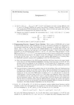

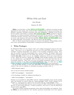
© Copyright 2026