1. No category

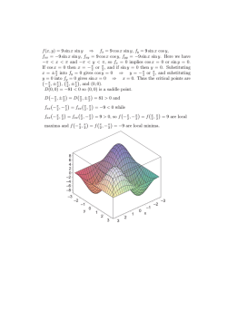
10.1515/acsc-2015-0019
Archives of Control Sciences
Volume 25(LXI), 2015
No. 3, pages 289–305
Topology optimization for elastic base under
rectangular plate subjected to moving load
SAMVEL H. JILAVYAN and ASATUR ZH. KHURSHUDYAN
Distribution optimization of elastic material under elastic isotropic rectangular thin plate
subjected to concentrated moving load is investigated in the present paper. The aim of optimization is to damp its vibrations in finite (fixed) time. Accepting Kirchhoff hypothesis with
respect to the plate and Winkler hypothesis with respect to the base, the mathematical model of
the problem is constructed as two–dimensional bilinear equation, i.e. linear in state and control
function. The maximal quantity of the base material is taken as optimality criterion to be minimized. The Fourier distributional transform and the Bubnov–Galerkin procedures are used to
reduce the problem to integral equality type constraints. The explicit solution in terms of two–
dimensional Heaviside‘s function is obtained, describing piecewise–continuous distribution of
the material. The determination of the switching points is reduced to a problem of nonlinear
programming. Data from numerical analysis are presented.
Key words: distributed system, moving load, Kirchhoff plate, Winkler base, topology optimization, problem of moments, L∞ -optimal control, distributions, Bubnov–Galerkin procedure.
1.
Introduction
The optimal design problems are traditionally considered in order to minimize or
maximize some parameters (weight, volume, load capacity and etc.) of a design with
given structure [1]. In the monograph [1] a wide range of construction optimization
problems of three main kinds: optimization of size, form and structure, are investigated.
Recently, the so–called design topology optimization problems have begun to be investigated in order to minimize a specific functional describing material distribution in
given domain, retaining or even improving desired properties of structures. The solution
of topology optimization problems, unlike problems of structural optimization, where
necessary conditions of optimality to be solved, are generally reduced to problem of
nonlinear programming (see, for example, [2, 3, 4, 5, 6, 7, 8, 15, 16, 18, 17] and the references therein). Nevertheless, the explicit analytical form determination for unknown
controls in such problems is connected with significant difficulties, and the numerical
The Authors are with Faculty of Mathematics and Mechanics, Yerevan State University. 1 Alex Manoogian str., 0025, Armenia. Correspondence Author is As. Zh. Khurshudyan, e-mail: [email protected]
To the blessed memory of innocent victims of Armenian Genocide (1915) is dedicated.
Received 08.05.2015.
Unauthenticated
Download Date | 10/2/16 8:26 PM
290
S.H. JILAVYAN, AS.ZH. KHURSHUDYAN
solution requires high computational costs. Topology optimization of a construction can
lead not only to an advantageous distribution of material in its volume, which is of direct practical importance, preserving or even optimizing its target properties; it also can
directly affect the processes in which it is involved. It opens further opportunities as in
engineering practice, as well as in manufacturing.
Such problems have not only practical importance, but stand out with complexity of
investigation, because mathematically they are formulated as bilinear control systems,
i.e. systems containing linear product of control and state function or their derivatives.
Such systems can be used to model a wide range of physical, chemical, biological processes that cannot be effectively modelled under the assumption of linearity (see [19]
and the references therein).
From the other hand side, vibration reduction and damping in particular systems
present a very important engineering problem. Besides the literature cited above we
refer to [9, 12, 14, 10, 13, 11] and the references therein. The investigation is devoted
to vibration reduction or damping for structures with actuators or absorbers having fixed
placements and configurations under it. In [8, 15, 16] we have attempted and here we
are going to attempt to damp bending vibrations of elastic structures (beam and plate)
by optimizing the way of placing the subgrade under those structures.
In general statement topology optimization problems require minimization of given
criterion
κ[u] →
− min, u ∈ U ,
u
describing as usual the distribution of material in design, by choosing u bounded by our
resources, under certain geometrical and characteristic constraints.
If, for example, the control problem is considered for a deformable design, equation
of its motion
Du [w] = f (xx,t), (xx,t) ∈ O × [0, T ],
(1)
(or static equilibrium) may be considered as characteristic (differential) constraints,
whereby x ∈ O ⊂ R3 will be the geometrical constraint. Besides, the solution of (1)
satisfies given conditions on boundary:
B [w] = w∂ (t), (xx,t) ∈ ∂O × [0, T ].
(2)
In dynamical problems some initial conditions at t = 0 moment are also considered. Main
purpose of control problem may be, for instance, ensuring given terminal conditions at
t = T moment.
The bilinear differential operator Du [w] is defined in O × [0, T ], B [·] is a linear or
nonlinear operator, representing the boundary conditions, f (xx,t) is a given function satisfying certain conditions.
Examples of operators Du [·] and B [·] may be found, for instance, in the above cited
literature and in [22, 23, 24, 20, 21].
Unauthenticated
Download Date | 10/2/16 8:26 PM
TOPOLOGY OPTIMIZATION FOR ELASTIC BASE UNDER RECTANGULAR PLATE
SUBJECTED TO MOVING LOAD
2.
We use the definitions
{
1, x > 0,
θ(x) =
0, x < 0,
291
Notations and abbreviations
{
1, x > 0 and y > 0,
θ(x, y) = θ(x)θ(y) =
0, otherwise,
for Heaviside‘s one and two-dimensional function, and δ = D θ for Dirac‘s delta function. The key technique we use to deal with distributions is their Fourier transform
[26, 27], defined in terms of direct
∫∞
Ft [η] := η(σ) =
η(t) exp [iσt] dt,
−∞
and inverse operators
Ft
−1
1
[η] =
2π
∫∞
η(σ) exp [−iσt] dσ = η(t),
−∞
σ ∈ R is the transform parameter. We use also the operators Fs−1 [·] and Fc−1 [·] for
Fourier inverse sine and cosine transforms
Fs−1 [η]
1
=
π
∫∞
η(σ) sin(σt)dσ,
0
Fc−1 [η]
1
=
π
∫∞
η(σ) cos(σt)dσ.
0
The Fourier transform of Dirac‘s delta F [δ(t − t0 )] = exp [iσt0 ] is used during computations below.
We use the filtering property of Dirac‘s delta
∫ε
δ(t − t0 )η(t)dt = η(t0 ), t0 ∈ (−ε, ε), ε > 0,
−ε
for all test functions η [27].
The following properties are also used throughout the paper without special reference [27]:
 (
)
(
)
x

−
1
, x0 > 0,
θ
1
x
x0 (
)
δ(x − x0 ) =
δ
− 1 , θ(x − x0 ) =
x0 ̸= 0,
1 − θ x − 1 , x0 < 0,
|x0 |
x0
x0
in the sense of distributions [27].
Unauthenticated
Download Date | 10/2/16 8:26 PM
292
S.H. JILAVYAN, AS.ZH. KHURSHUDYAN
D is the bending stiffness of the plate, ∆ is the two–dimensional Laplacian,
δµm = δm
µ =
∫π
−π
{
1, m = µ,
sin(πmx) sin(πµx)dx =
0, m =
̸ µ,
µ ν
δµν
mn = δm δn ,
are the Kronecker one and two-dimensional symbols. For short we write {1; N} instead
of {1, 2, . . . , N}.
The operator A[a,b] [·], introduced in [8, 15, 16, 25, 28], is defined as follows
{
η(t), t ∈ [a, b],
A[a,b] [η] =
0, t ∈
/ [a, b].
It obviously may be represented in terms of characteristic function of [a, b]
{
1, t ∈ [a, b],
χ[a,b] (t) =
0, t ∈
/ [a, b],
as follows
A[a,b] [η] = χ[a,b] (t)η(t) := η1 (t),
but it is more convenient to use the representation [8, 15, 16, 25, 28]
A[a,b] [η] = [θ(t − a) − θ(t − b)] η(t).
supp η = {x ∈ R; η(x) ̸= 0} denotes the support of η. It is obvious that supp A[a,b] [η] =
[a, b].
Remark 1 The above introduced operator A[a,b] [·] is a linear continuous mapping from
the space of ordinary functions into the Sobolev space of functions, which are concentrated on [a, b] and has distributional derivatives of any order.
The derivatives of η may be expressed in terms of distributional derivatives of η1 =
A[a,b] [η]:
n−1
[
]
D n η1 (t) = A[a,b] [D n η] + ∑ Cnν D ν η(a)D n−ν−1 δ(t − a) − D ν η(b)D n−ν−1 δ(t − b) ,
ν=1
(Cmn are the binomial coefficients).
Unauthenticated
Download Date | 10/2/16 8:26 PM
TOPOLOGY OPTIMIZATION FOR ELASTIC BASE UNDER RECTANGULAR PLATE
SUBJECTED TO MOVING LOAD
3.
293
The method of solution
In order to solve the bilinear control problems when B [·] is linear we suggest [15] to
use the Bubnov–Galerkin procedure [29]. Suppose, that we have constructed a complete
system of basis (approximating) functions {φn (xx)}Nn=0 , the first one of which satisfies
non–homogeneous, and the rest– to homogeneous boundary conditions (2). Then the
residual, obtained as a result of substitution of approximate solution
N
wN (xx,t) = ε0 (t)φ0 (xx) + ∑ εn (t)φn (xx), (xx,t) ∈ O × [0, T ],
(3)
n=1
where the coefficients εn (t) should be determined, t is considered as a parameter, into
(1.1), will be
(4)
RN (xx,t) = Du [wN ] − f (xx,t), (xx,t) ∈ O × [0, T ].
According to the Bubnov–Galerkin procedure, the unknown coefficients ε(t) are
determined from orthogonality conditions of the residual (4) and basis functions
{φn (xx) }Nn=0
∫
RN (xx,t)φn (xx)dxx = 0, t ∈ [0, T ], n ∈ {0; N}.
(5)
O
Remark 2 If for some N0 ∈ N the residual (4) is identically zero: RN0 (xx,t) ≡ 0, then the
corresponding function wN0 (xx,t) (3) will be the exact solution of boundary–value problem (1), (2). Otherwise, increasing the number N of approximating functions {φn (xx)}Nn=0
we may increase the accuracy of approximation (3).
After determining the unknown coefficients εn (t) from the system of linear equations
(5) and substituting them into (3), and taking into account, that at T given terminal
conditions must be satisfied, we will derive the system
N
wN (xx, T ) = ε0 (T )φ0 (xx) + ∑ εn (T )φn (xx), x ∈ O .
n=1
Then, the unknown function u has to be determined from
wnNT = εn (T ), n ∈ {0; N}
(6)
∫
in which
wnNT
wN (x, T )φn (xx)dxx.
=
O
Remark 3
i) Naturally, we should put the subscript N to the unknown u to underline that it is
an approximation, but we omit it implying the dependence obvious.
Unauthenticated
Download Date | 10/2/16 8:26 PM
294
S.H. JILAVYAN, AS.ZH. KHURSHUDYAN
ii) The complexity of the technique application depends on complexity of operator
Du [·] and, especially, its component with respect to t: it defines the type (algebraic,
differential, integral, integro-differential etc.) of (5) for εn (t).
4. The problem statement
In this section we are going to apply the technique described in the previous section
for a two–dimensional bilinear system. We consider an elastic, isotropic, solid rectangular plate of sufficiently small constant thickness 2h, the middle plane of which in
Cartesian system of coordinates occupies the domain
O∗ = {(x∗ , y∗ ); x∗ ∈ [−l1 , l1 ], y∗ ∈ [−l2 , l2 ]} ⊂ R2 , min(l1 , l2 ) ≫ 2h.
Let the plate lies on a linear–elastic one–parametric base with substrate ratio α2∗ , distributed in O∗ by a controlled law u = u(x, y). The plate is supposed to be simply supported by edges x∗ = ±l1 and y∗ = ±l2 , as well as subjected to a constant normal load P∗
distributed on the upper surface of the plate by given law r∗ = r∗ (y∗ ), supp r∗ ̸= ∅, and
moving along the upper surface of the plate in x∗ direction with constant velocity v∗ .
We accept the Kirchhoff hypothesis with respect to the plate and the Winkler hypothesis with respect to the elastic base. Then, the vertical displacements of the plate
middle plane satisfy
D∆∆w∗ (x∗ , y∗ ,t∗ ) + α2∗ u(x∗ , y∗ )w∗ (x∗ , y∗ ,t∗ ) + 2ρh
∂2 w∗ (x∗ , y∗ ,t∗ )
= f∗ (x∗ , y∗ ,t∗ ), (7)
∂t∗2
(x∗ , y∗ ,t∗ ) ∈ O∗ × (0, T ),
and the boundary conditions of simply supported edges
∂2 w∗ (x∗ , y∗ ,t∗ ) w∗ (±l1 , y∗ ,t∗ ) =
= 0, (y∗ ,t∗ ) ∈ [−l2 , l2 ] × [0, T ],
∂x∗2
x∗ =±l1
∂2 w∗ (x∗ , y∗ ,t∗ ) w∗ (x∗ , ±l2 ,t∗ ) =
= 0, (x∗ ,t∗ ) ∈ [−l1 , l1 ] × [0, T ].
∂y2
∗
(8)
y∗ =±l2
Above u is the law of the elastic base distribution in O∗ , f∗ (x∗ , y∗ ,t∗ ) characterizes
the impact of the moving load on the plate:
f∗ (x∗ , y∗ ,t∗ ) = P∗ A[0,τ∗ ] [δ(x∗ + l1 − v∗t∗ )]r∗ (y∗ ).
(9)
The initial state of the plate is known:
∂w∗ (x∗ , y∗ ,t∗ ) = w10∗ (x∗ , y∗ ), (x∗ , y∗ ) ∈ O∗ .
w∗ (x∗ , y∗ , 0) = w0∗ (x∗ , y∗ ),
∂t∗
t∗ =0
(10)
Unauthenticated
Download Date | 10/2/16 8:26 PM
TOPOLOGY OPTIMIZATION FOR ELASTIC BASE UNDER RECTANGULAR PLATE
SUBJECTED TO MOVING LOAD
295
Our main purpose is the determination of an admissible control uo ∈ U = {0 ¬ u ∈
|u| ¬ 1, supp u ⊆ O∗ } providing the following terminal state in required (fixed)
time T :
∂w∗ (x∗ , y∗ ,t∗ ) w∗ (x∗ , y∗ , T ) = 0,
= 0, (x∗ , y∗ ) ∈ O∗ ,
(11)
∂t∗
t∗ =T
L∞ (O∗ );
as well as minimizing intensity of the elastic base distribution under the plate described
by the functional
κ[u] = max |u(x∗ , y∗ )|, u ∈ U .
(12)
(x∗ ,y∗ )∈O∗
Remark 4 It is obvious that the plate vibrations may "vanish" solely after the load detaches from it. Thence we suppose that the load detaches from the plate at a given moment τ∗ < T , such that v∗ τ∗ = 2l1 . Naturally, we have to restrict us by condition T < T0 ,
where T0 is the time in which the vibrations will "vanish" in the case of u(x, y) ≡ 1.
We realize that, in general, terminal conditions (11) may not be provided by choice
of any distribution u (even in the case u ≡ 1) exactly, because there will remain some
residual stresses of very small amplitude inversely proportional to the base stiffness.
Thus, we deal with a problem of approximate controllability, i.e. equality signs in (11)
are, actually, approximate equalities.
We additionally suppose, that the consistency conditions concerning boundary, initial and terminal data are satisfied:
w0∗ (±l1 , y∗ ) = w0∗ (x∗ , ±l2 ) = 0, w10∗ (±l1 , y∗ ) = w10∗ (x∗ , ±l2 ) = 0,
∂2 w0∗ (x∗ , y∗ ) ∂2 w0∗ (x∗ , y∗ ) =
= 0.
∂x∗2
∂y2∗
x∗ =±l1
y∗ =±l2
Before proceeding to the control problem solution, let us transform (7)-(12) introducing the dimensionless variables and functions
w=
w∗
r∗
x∗
y∗
2t∗ − T
2ϑ
v∗ T
, r= , x= , y= , t =
ϑ, τ =
τ∗ , v =
,
h
l2
l1
d
T
T
l1 2ϑ
( )
Pdl13
l14 2ϑ 2
l1
α2∗ l14 2
2
, β = 2ρh
, γ = , P∗ =
.
α =
D
D T
l2
Dh
Then, we will obtain
∂2 w(x, y,t)
= f (x, y,t), (x, y,t) ∈ O × (−ϑ, ϑ),
∂t 2
∂2 w(x, y,t) w(±1, y,t) =
= 0, (y,t) ∈ [−1, 1] × [−ϑ, ϑ],
∂x2
x=±1
∂2 w(x, y,t) = 0, (x,t) ∈ [−1, 1] × [−ϑ, ϑ],
w(x, ±1,t) =
∂y2
y=±1
D [w] + α2 u(x, y)w(x, y,t) + β2
(13)
(14)
Unauthenticated
Download Date | 10/2/16 8:26 PM
296
S.H. JILAVYAN, AS.ZH. KHURSHUDYAN
D [w] =
4
4
∂4 w(x, y,t)
2 ∂ w(x, y,t)
4 ∂ w(x, y,t)
+
2γ
+
γ
,
∂x4
∂x2 ∂y2
∂y4
O := (−1, 1) × (−1, 1).
As a result of the variables change, the expression (9) transforms to
f (x, y,t) = PA[−ϑ,ϑ−τ] [δ(x + 1 − v(t + ϑ))] r(y).
In order to deal with control problem under study we are aimed to use the
Butkovskiy‘s generalized method, suggested in [25, 28]. For that purpose we apply the
operator A[−ϑ,ϑ] [·] to (10) and (11). Taking into account that in the sense of distributions
[θ(t + ϑ) − θ(t − ϑ)]
∂w(x, y,t)
∂2 w(x, y,t) ∂2 w1 (x, y,t)
=
− [δ(t + ϑ) − δ(t − ϑ)]
−
2
2
∂t
∂t
∂t
− [δ′ (t + ϑ) − δ′ (t − ϑ)]w(x, y,t) =
=
∂2 w1 (x, y,t)
− w10 (x, y)δ(t + ϑ) − w0 (x, y)δ′ (t + ϑ),
∂t 2
we will arrive at
∂2 w1 (x, y,t)
= G(x, y,t), (x, y,t) ∈ O × R,
∂t 2
∂2 w1 (x, y,t) w1 (±1, y,t) =
= 0, (y,t) ∈ [−1, 1] × R,
∂x2
x=±1
∂2 w1 (x, y,t) w1 (x, ±1,t) =
= 0, (x,t) ∈ [−1, 1] × R,
∂y2
y=±1
D [w1 ] + α2 u(x, y)w1 (x, y,t) + β2
where
(15)
(16)
G(x, y,t) = f1 (x, y,t) + β2 [w0 (x, y)δ′ (t) + w10 (x, y)δ(t)].
Applying now the Fourier transform with respect to t variable to system (15), (16),
we will obtain
[
]
D [w1 ] + α2 u(x, y) − σ2 β2 w1 (x, y, σ) = G(x, y, σ), (x, y, σ) ∈ O × R, (17)
∂2 w1 (x, y, σ) w1 (±1, y, σ) =
= 0, (y, σ) ∈ [−1, 1] × R,
∂x2
x=±1
(18)
∂2 w1 (x, y, σ) w1 (x, ±1, σ) =
= 0, (x, σ) ∈ [−1, 1] × R,
∂x2
y=±1
G(x, y, σ) = f 1 (x, y, σ) + β2 [w101 (x, y) − iσw01 (x, y)],
[ (
)]
x+1
P
+ ϑ r(y).
f 1 (x, y, σ) = [θ(x + 1) − θ(x − 1)] exp iσ
v
v
Unauthenticated
Download Date | 10/2/16 8:26 PM
TOPOLOGY OPTIMIZATION FOR ELASTIC BASE UNDER RECTANGULAR PLATE
SUBJECTED TO MOVING LOAD
297
It is taken into account here that vτ = 2.
In order to solve this problem we aimed to apply the Bubnov–Galerkin procedure.
Orthonormal in O system of functions {sin(πmx) sin(πny)}m,n∈N , is, obviously, approximating for boundary value problem (17), (18), and therefore we may look its solution
for as follows:
N
∑
w1N (x, y, σ) =
εmn (σ) sin(πmx) sin(πny), (x, y, σ) ∈ O × R,
(19)
m,n=1
where εmn (σ) are unknown yet. Applying the procedure described above, we will derive
the following system of linear algebraic equations for εmn (σ):
N
∑
Λµν
mn (σ)εmn (σ) = Ωµν (σ), µ, ν ∈ {1; N},
(20)
m,n=1
where
[
]
µν
2 µν
2
2
2 2
Λµν
− σ 2 β2 ,
mn (σ) = Γmn δmn + α Jmn [u], Γmn = (πm) + γ (πn)
∫1 ∫1
µν
Jmn
[u]
=
u(x, y) sin(πmx) sin(πµx) sin(πny) sin(πνy)dxdy,
−1 −1
Ωµν (σ) = Yµ (σ)
∫1
r(y) sin(πνy)dxdy + β2 [Kµν − iσLµν ] ,
−1
[
[
]]
(−1)µ+1 πµ · Pv
2iσ
Yµ (σ) =
1 − exp
exp [iσϑ] ,
σ2 + (πµv)2
v
∫1 ∫1
w101 (x, y) sin(πµx) sin(πνy)dxdy,
Kµν =
−1 −1
∫1 ∫1
Lµν =
w01 (x, y) sin(πµx) sin(πνy)dxdy.
−1 −1
It is obvious, that
mn [u]
Jmn
µν
νµ
­ 0, Jmn [u] = Jnm [u], m, n, µ, ν ∈ {1; N}.
Remark 5 Since the Chebyshev polynomials of the first kind {Tm (x)Tn (y)}m,n∈N are
orthogonal in O and provide more accuracy of approximation compare with that by
trigonometric system {sin(πmx) sin(πny)}m,n∈N [29], it is more efficient to use them
instead. But we take into account, that the aim is to show that the proposed algorithm
works in dimensions two, and not the accuracy of the approximation.
Unauthenticated
Download Date | 10/2/16 8:26 PM
298
S.H. JILAVYAN, AS.ZH. KHURSHUDYAN
Since w1 (x, y,t) ≡ A[−ϑ,ϑ] [w] by the definition is compactly supported in [−ϑ, ϑ],
then, according to Wiener–Paley–Schwartz theorem [26, 27], the extension w1 (x, σ + iς),
ς ∈ R, is entire. It means, that ∆11 (z) = 0, as long as ∆0 (z) = 0, where ∆0 and ∆11 are the
main and (for instance) the first auxiliary determinants of (20), respectively.
Remark 6
µν
i) It is easy to see from the expression of Λmn , the determinant ∆0 (σ) is a polynomial
of degree 2N, therefore ∆0 (z) = 0 admits 2N complex roots. From the other hand
side
Re ∆0 (−σ − iς) = Re ∆0 (σ + iς), Im ∆0 (−σ − iς) = Im ∆0 (σ + iς),
which means that zk = σk + iςk and zk = −σk − iςk satisfy ∆0 (z) = 0 simultaneously. Then, since
Re ∆11 (−σ − iς) = Re ∆11 (σ + iς), Im ∆11 (−σ − iς) = Im ∆11 (σ + iς),
we conclude that ∆11 (z) = 0 contains only N independent conditions.
ii) Moreover, even though
Re ∆0 (−σ + iς) = Re ∆0 (σ − iς) = Re ∆0 (σ + iς)
Im ∆0 (−σ + iς) = Im ∆0 (σ − iς) = −Im ∆0 (σ + iς),
nevertheless ∆11 (σ + iς) does not have the same property, therefore the number of
independent equalities cannot be reduced further.
Suppose that we were able to solve ∆0 (z) = 0 and find the roots zk , k ∈ {1; N}. Substituting them into ∆11 (z) = 0 and separating its real and imaginary parts, with respect
µν
to Jmn [u] we will obtain the system of restrictions
µν
µν
Jmn
[u] = Mmn
, m, n, µ, ν ∈ {1; N},
According to [17, 28], the solution will be
J
uo (x, y) =
∑
[ (
)
(
)]
θ x − xoj , y − yoj − θ x − xoj+1 , y − yoj+1 , (x, y) ∈ O .
(21)
j=1
The obtained solution describes the distribution law of the elastic base under the plate,
and the set of points {xoj , yoj }Jj=1 ∈ O underlines the domains where the base exists and
depends on inner and external parameters D, r(y), v, τ, P, α2 , β2 , γ.
After determination of optimal solution (21), we might need also the optimal deflection of the plate. Applying the Fourier inverse transform to (19)we will obtain
N
w1N (x, y,t) =
∑
εmn (t) sin(πmx) sin(πny), (x, y,t) ∈ O × R,
(22)
m,n=1
Unauthenticated
Download Date | 10/2/16 8:26 PM
TOPOLOGY OPTIMIZATION FOR ELASTIC BASE UNDER RECTANGULAR PLATE
SUBJECTED TO MOVING LOAD
299
Remark 7 Taking into account that
µν
Λµν
mn (−σ) = Λmn (σ), Re Ωµν (−σ) = Re Ωµν (σ),
Im Ωµν (−σ) = −Im Ωµν (σ),
we see that
Re εmn (−σ) = Re εmn (σ), Im εmn (−σ) = −Im εmn (σ).
It is necessary and sufficient for εmn (t) = Ft −1 [εmn ], and therefore for w1N (x, y,t), to be
real valued. Then,
1
εmn (t) =
π
∫∞
[Re εmn (σ) cos(σt) + Im εmn (σ) sin(σt)] dσ = Fc−1 [Re εmn ]+ Fs−1 [Im εmn ],
0
where
Re εmn (σ) =
Re ∆mn (σ)Re ∆0 (σ) + Im ∆mn (σ)Im ∆0 (σ)
(Re ∆0 (σ))2 + (Im ∆0 (σ))2
,
Re ∆mn (σ)Im ∆0 (σ) − Im ∆mn (σ)Re ∆0 (σ)
Im εmn (σ) = −
(Re ∆0 (σ))2 + (Im ∆0 (σ))2
5.
.
Numerics
To demonstrate the procedure of the switching points calculation, let us consider a
numerical experiment. Let
w01 (x, y) = sin(πx) sin(πy), ẇ01 (x, y) = 0.
We additionally assume, that the moving load has a point support: r(y) = δ(y − y0 ),
y0 ∈ (−1, 1). Then, limiting the consideration by N = 3 we have the results combined in
Figures 1 and 2 and in Tables 1–3 for various values of dimensionless parameters D, α2 ,
β2 , γ, P, v, τ. Poisson‘s ratio of the plate material is taken equal to 0.25.
Since the expressions for ∆0 and ∆11 are unwieldy and it is useless to bring them
here, we bring the expressions for
J
µν
Jmn
[u] =
∑
j=1
xo
∫j+1
yo
∫j+1
sin(πny) sin(πνy)dy,
sin(πmx) sin(πµx)dx
xoj
yoj
[
[ ]]
(−1)µ+1 πµ · vP
2iz
µ
Ωµν (z) = 2
1 − exp
exp [izϑ] · sin(πνy0 ) − izβ2 δ1 δν1 ,
2
z + (πµv)
v
Unauthenticated
Download Date | 10/2/16 8:26 PM
300
S.H. JILAVYAN, AS.ZH. KHURSHUDYAN
Table 2: β2 = 50, γ = 0.25
α2
P
v
τ
y0
x1o
yo1
x2o
yo2
x3o
yo3
x4o
yo4
0.01
0.1
0.01
100
-0.25
0.1973
0.3307
0.2650
0.4931
0.2691
0.5330
0.3355
0.6699
0.01
0.5
0.05
150
0.5
−0.4444
−0.4444
−0.2989
−0.2989
0.3074
0.3074
0.4349
0.4349
0.05
0.1
0.01
100
0.25
−0.7264
−0.7809
−0.5139
−0.4936
−0.0475
−0.0077
0.0969
0.1864
0.05
0.5
0.1
150
0.25
−0.4167
−0.4167
−0.2703
−0.2703,
0.3270
0.3270
0.4466
0.4466
0.1
0.1
0.1
100
-0.5
−0.7557
−0.5619
0.1406
0.0554
0.5143
0.4113
0.7555
0.9799
0.1
0.5
0.1
150
0.5
−0.4371
−0.4371
−0.2963
−0.2963
0.3042
0.3042
0.4282
0.4282
Table 3: β2 = 25, γ = 1
α2
P
v
τ
y0
x1o
yo1
x2o
yo2
x3o
yo3
x4o
yo4
0.01
0.1
0.01
100
0.25
−0.8376
−0.9815
−0.6615
−0.4452
0.6087
−0.3912
0.6897
0.0556
0.01
0.5
0.05
150
-0.75
−0.4146
−0.4146
−0.2677
−0.2677
0.3283
0.3283
0.4349
0.4477
0.05
0.1
0.01
100
-0.1
−0.2748
−0.3973
−0.2709
−0.2035
0.5555
0.2735
0.7504
0.3567
0.05
0.5
0.1
150
0.1
−0.4421
−0.4421
−0.2965
−0.2965
0.2926
0.2926
0.4228
0.4228
0.1
0.1
0.05
100
0.4
−0.2065
−0.2984
−0.1324
−0.2968
0.4080
0.3931
0.4781
0.3943
0.1
0.5
0.1
150
0.1
−0.4211
−0.4211
−0.2759
−0.2759
0.3234
0.3233
0.4437
0.4437
Unauthenticated
Download Date | 10/2/16 8:26 PM
TOPOLOGY OPTIMIZATION FOR ELASTIC BASE UNDER RECTANGULAR PLATE
SUBJECTED TO MOVING LOAD
301
Figure 1: uo (x, y) when β2 = 50, γ = 0.25, α2 = 0.05, P = 0.5, v = 0.1, τ = 150 and y0 =
0.25.
Figure 2: uo (x, y) when β2 = 25, γ = 1, α2 = 0.01, P = 0.5, v = 0.05, τ = 150 and y0 =
−0.75
Unauthenticated
Download Date | 10/2/16 8:26 PM
302
S.H. JILAVYAN, AS.ZH. KHURSHUDYAN
Table 4: β2 = 20, γ = 2
α2
P
v
τ
y0
x1o
yo1
x2o
yo2
x3o
yo3
x4o
yo4
0.01
0.1
0.01
100
0.25
−0.4258
−0.3881
−0.2114
−0.2724
0.3054
= 0.4269
0.4408,
0.4270
0.01
0.5
0.05
150
-0.75
−0.4389
−0.4146
−0.2925
−0.2925
0.3025
0.3025
0.4308,
0.4308
0.05
0.1
0.05
100
-0.4
−0.4360
−0.4360
−0.2888
−0.2888
0.3136
0.3136
0.4399,
0.4399
0.05
0.5
0.1
150
0.4
−0.4105
−0.3583
−0.1466
−0.3567
0.4508
0.4778
0.5467,
0.5478
0.1
0.1
0.01
100
0.25
−0.4456
−0.3596
−0.2521
−0.2483
0.4542
0.2450
0.4566
0.46
0.1
0.5
0.1
150
-0.25
−0.2776
−0.1503
0.0706
−0.1494
0.4388
0.5020
0.5237,
0.5192
6. Conclusion
The solution of distribution optimization problem for elastic material in rectangular domain is obtained explicitly using the Butkovskiy‘s generalized method and the
Bubnov–Galerkin procedure in turn. The aim is the minimization of the material quantity in order to damp the bending vibrations of a simply supported isotropic elastic plate
caused by a moving load in required time. The mathematical model is constructed as
a bilinear partial differential equation of fourth order. Introducing a new, generalized
state function, the state equation is written in the class of distributions and the initial
conditions are included in it. Involving the Fourier distributional transform, the governing system is reduced to a boundary–value problem for partial differential equation with
two independent variables. The solution is approximated by means of Bubnov–Galerkin
orthonormal sequence and with respect to approximation coefficients a system of algebraic equations is obtained. Those coefficients are found and extended in C as entire
functions. Resolving conditions (necessary and sufficient) are the zeros of one of the
auxiliary determinants extended in C in roots of the main determinant extended in C.
It turns out that the piecewise–continuous distribution of the material is optimal and is
determined uniquely via solution of a problem of nonlinear programming. Numerical
analysis is done for a particular initial state and for various values of the system internal
and external parameters.
Unauthenticated
Download Date | 10/2/16 8:26 PM
TOPOLOGY OPTIMIZATION FOR ELASTIC BASE UNDER RECTANGULAR PLATE
SUBJECTED TO MOVING LOAD
303
References
[1] P.W. C HRISTENSEN and A. K LARBRING: An Introduction to Structural Optimization. Solid Mechanics and its Applications. Springer, Berlin, 2009.
[2] M.P. B ENDSO
/E and O. S IGMUND: Topology Pptimization. Theory, Methods and
Applications. Springer, Berlin, 2003.
[3] P.A. B ROWNE: Topology optimization of linear elastic structures. Thesis submitted for the PhD degree, Bath, 2013.
[4] H.A. E SCHENAUER and N. O LHOFF: Topology optimization of continuum structures: A review. ASME Applied Mechanics Reviews, 54(4), (2001), 331-390.
[5] J. H ASLINGER and P. N EITTAANMÄKI: Finite Element Approximation for Optimal Shape, Material and Topology Design. 2nd edition. Wiley, New York, 1996.
[6] J. H ASLINGER and R.A.E. M ÄKINEN: Introduction to Shape Optimization: Theory, Approximation, and Computation. Advances in Design and Control. SIAM,
Philadelphia, 2003.
[7] J. H ASLINGER , J. M Á LEK and J. S TEBEL: A new approach for simultaneous
shape and topology optimization based on dynamic implicit surface function. Control and Cybernetics, 34(1), (2005), 283-303.
[8] S.H. J ILAVYAN , A S .Z H . K HURSHUDYAN and A.S. S ARKISYAN: On adhesive
binding optimization of elastic homogeneous rod to a fixed rigid base as a control
problem by coefficient. Archives of Control Sciences, 23(4), (2013), 413-425.
[9] P.M. P RZYBYLOWICZ: Active reduction of resonant vibration in rotating shafts
made of piezoelectric composites. Archives of Control Sciences, 13(3), (2003), 327337.
[10] Z. G OSIEWSKI and A. S OCHACKI: Control system of beam vibration using piezo
elements. Archives of Control Sciences, 13(3), (2003), 375-385.
[11] L. L ENIOWSKA and R. L ENIOWSKI: Active control of circular plate vibration by
using piezoceramic actuators. Archives of Control Sciences, 13(4), (2003), 445457.
[12] A. B RANSKI and S. S ZELA: On the quasi optimal distribution of PZTs in active
reduction of the triangular plate vibration. Archives of Control Sciences, 17(4),
(2007), 427-437.
[13] Z. G OSIEWSKI and A. S OCHACKI: Optimal control of active rotor suspension
system. Archives of Control Sciences, 17(4), (2007), 459-468.
Unauthenticated
Download Date | 10/2/16 8:26 PM
304
S.H. JILAVYAN, AS.ZH. KHURSHUDYAN
[14] L. S TAREK , D. S TAREK , P. S OLEK and A. S TAREKOVA: Suppression of vibration
with optimal actuators and sensors placement. Archives of Control Sciences, 20(1),
(2010), 99-120.
[15] A S .Z H . K HURSHUDYAN: The Bubnov–Galerkin procedure in bilinear control
problems. Automation and Remote Control, 76(8), (2015), 1361-1368.
[16] A M .Z H . K HURSHUDYAN and A S .Z H . K HURSHUDYAN: Optimal distribution of
viscoelastic dampers under elastic finite beam under moving load. Proc. of NAS of
Armenia, 67(3), (2014), 56-67 (in Russian).
[17] S.V. S ARKISYAN , S.H. J ILAVYAN and A S .Z H . K HURSHUDYAN: Structural optimization for infinite non homogeneous layer in periodic wave propagation problems. Composite Mechanics, 51(3), (2015), 277–284.
[18] L.C. N ECHES and A.P. C ISILINO: Topology optimization of 2D elastic structures
using boundary elements. Engineering Analysis with Boundary Elements, 32(7),
(2008), 533-544.
[19] P.M. PARDALOS and V. YATSENKO: Optimization and Control of Bilinear Systems. Springer, Berlin, 2008.
[20] K. B EAUCHARD and P. ROUCHON: Bilinear control of Schrodinger PDEs. In Encyclopedia of Systems and Control, 24 (to appear in 2015).
[21] M.E. B RADLEY and S. L ENHART: Bilinear optimal control of a Kirchhoff plate.
Systems & Control Letters, 22(1), (1994), 27-38.
[22] V.F. K ROTOV, A.V. B ULATOV and O.V. BATURINA: Optimization of linear systems with controllable coefficients. Automation and Remote Control, 72(6), (2011),
1199-1212.
[23] I.V. R ASINA and O.V. BATURINA: Control optimization in bilinear systems. Automation and Remote Control, 74(5), (2013), 802-810.
[24] M. O UZAHRA: Controllability of the wave equation with bilinear controls. European J. of Control, 20(2), (2014), 57-63.
[25] A S .Z H . K HURSHUDYAN: Generalized control with compact support of wave equation with variable coefficients. International J. of Dynamics and Control, (2015),
DOI: 10.1007/s40435-015-0148-3.
[26] V.S. V LADIMIROV: Methods of the Theory of Generalized Functions. Analytical
Methods and Special Functions. CRC Press, London-NY, 2002.
[27] A.H. Z EMANIAN: Distribution Theory and Transform Analysis: An Introduction
to Generalized Functions, with Applications. Dover Publications, New York, 2010.
Unauthenticated
Download Date | 10/2/16 8:26 PM
TOPOLOGY OPTIMIZATION FOR ELASTIC BASE UNDER RECTANGULAR PLATE
SUBJECTED TO MOVING LOAD
305
[28] A S .Z H . K HURSHUDYAN: Generalized control with compact support for systems
with distributed parameters. Archives of Control Sciences, 25(1), (2015), 5-20.
[29] S.G. M IKHLIN: Error Analysis in Numerical Processes. John Wiley & Sons Ltd,
New York, 1991.
Unauthenticated
Download Date | 10/2/16 8:26 PM