
On the Asymptotic Determination of Invariant Manifolds for
Rev. Real Academia de Ciencias. Zaragoza. 57: 7–66, (2002).
On the Asymptotic Determination of Invariant Manifolds for
Autonomous Ordinary Differential Equations
Jes´
us Palaci´an
Departamento de Matem´atica e Inform´
atica.
Universidad P´
ublica de Navarra. E – 31006 Pamplona. Spain.
Premio de la Academia a la Investigaci´on (2001–02)
Abstract
A methodology to calculate the approximate invariant manifolds of dynamical systems defined through an m–dimensional autonomous vector field is presented. The
technique is based on the calculation of formal symmetries and generalized normal
forms associated to the vector field making use of Lie transformations for ordinary
differential equations. Once a symmetry is determined up to a certain order, a reduction map allows us to pass from the equation in normal form to the orbit space,
leading to the so–called reduced system of dimension s < m. Next, a non–degenerate
p–dimensional invariant set of the reduced system is transformed, asymptotically, into a
(p+m−s)–dimensional invariant set of the departure equation. We put three examples
of normal forms computations and reduction process for Hamiltonian and dissipative
systems. The procedure is illustrated by three applications: i) we characterize the set of
all periodic orbits sufficiently close to the origin of the Hamiltonian vector field defined
by the H´enon and Heiles family when the main frequencies do not satisfy a resonance
condition; ii) we calculate the normally hyperbolic invariant manifold together with
its stable and unstable manifold of an equilibrium point of type centre×centre×saddle
for the three–degrees–of–freedom (3DOF) Hamilton function of the Rydberg atom, explaining the relevance of these invariant structures in the Transition State Theory; and
iii) we apply our technique to the reduction process of the Lorenz equations, obtaining
periodic orbits and some one–dimensional (1D) and 2D invariant sets.
Key words and expressions: Extended normal forms, Lie transformations, homology equation, invariant theory, mapping reductions, orbit spaces, reduced phase
spaces, centre reduction, periodic orbits, nD invariant tori, normally hyperbolic invariant manifolds, Transition State Theory, averaging techniques, Hamiltonian functions,
dissipative systems.
7
AMS (MOS) Subject Classification: 34C20, 34C14, 34C25, 34K19, 37J15, 37J40.
Resumen
En este trabajo se presenta una metodolog´ıa para calcular variedades invariantes
de un sistema din´
amico definido mediante un sistema de m ecuaciones diferenciales
aut´onomas. La t´ecnica que empleamos se basa en el c´alculo de simetr´ıas asint´oticas y
formas normales generalizadas asociadas al campo vectorial que define la ecuaci´on de
origen, haciendo uso de transformaciones de Lie para ecuaciones diferenciales ordinarias. Una vez determinada la simetr´ıa hasta un cierto orden de aproximaci´on un proceso
de reducci´
on permite formular la ecuaci´on transformada en un espacio de dimensi´on
s, estrictamente menor que m. El resultado central del trabajo establece que, bajo
ciertas condiciones de regularidad, una variedad de dimensi´on p, invariante por el flujo
del sistema din´
amico correspondiente al sistema de ecuaciones reducido, se transforma
mediante el cambio inverso al anterior, en otra variedad de dimensi´on p + m − s que
es aproximadamente invariante por el flujo del sistema din´amico correspondiente a la
ecuaci´
on de partida. Adem´
as en el caso de que las variedades sean toros invariantes,
la transformaci´
on asegura la existencia de toros invariantes de dimensi´on p + m − s
en el sistema original. La teor´ıa desarrollada se ilustra a trav´es de tres aplicaciones:
i) caracterizamos el conjunto de todas las ´orbitas peri´odicas suficientemente cercanas
al origen, de un problema de din´amica gal´actica, en el que las frecuencias principales
del sistema original no satisfacen una condici´on de resonancia; ii) calculamos la variedad invariante normalmente hiperb´olica as´ı como sus variedades estable e inestable
de un punto cr´ıtico cuya estabilidad es de tipo centro×centro×silla correspondiente a
un hamiltoniano de tres grados de libertad que modeliza la trayectoria de un ´atomo
sujeto a la acci´
on de un campo el´ectrico y otro magn´etico dispuestos en direcciones
perpendiculares, explicando la relevancia que tienen las estructuras geom´etricas invariantes en el lenguaje de la teor´ıa del estado de transici´on en reacciones qu´ımicas; y
iii) aplicamos la teor´ıa al estudio del sistema disipativo de origen metereol´ogico, llamada ecuaci´
on de Lorenz, obteniendo nuevas variedades invariantes de dimens´on dos
y ´orbitas peri´
odicas, para ciertos valores de los par´ametros del problema.
Palabras clave y expresiones: Formas normales extendidas, transformaciones de
Lie, ecuaci´
on homol´
ogica, teor´ıa de invariantes, aplicaciones de reducci´on, espacios orbitales, espacios f´
asicos reducidos, reducci´on a la variedad central, trayectorias peri´odicas, toros invariantes n–dimensionales, variedades invariantes normalmente hiperb´olicas, teor´ıa del estado de transici´on, t´ecnicas de promedios, funciones hamiltonianas,
sistemas disipativos.
8
1
Introduction and scope of the paper
The general setting of this paper is given through ordinary differential equations having the
form
d x(t)
= F(x(t); ε) =
dt
L
εi
Fi (x(t)),
i=0 i!
(1)
where t represents the independent variable, x ∈ Rm , ε stands for a dimensionless small
parameter and for 0 ≤ i ≤ L, Fi is a vector field with m components defined on an open set
Ω ⊆ Rm . Note that L can be interpreted as the degree reached by the Taylor development
of an analytic vector field, thus it can be infinity.
In particular, if F has a canonical character, there is a scalar field H such that Equa-
tion (1) is equivalent to
L
H(q(t), p(t); ε) =
εi
Hi (q(t), p(t)).
i=0 i!
(2)
Many dynamical systems are modelled by a system of ordinary differential equations either
of the type (1) or of the type (2). In both cases they are normally formed by the sum
of a principal part (F0 or H0 ) plus the perturbation. These equations are very typical of
Dynamical Systems Theory; for instance in stability and bifurcation analysis of equilibrium
points, periodic orbits or singularity theories. Since (2) is a particular situation of (1) we
shall present the results for the more general case, particularizing for (2) when dealing with
Hamilton functions.
Analytical methods that deal with dynamical systems like (1) are based on the fact that
the vector field
L
i
i=1 (ε /i!) Fi
corresponds to a small perturbation of the principal part F0 .
In the context of Perturbation Theory [25, 33] our aim is to transform the initial problem
to a simpler one by means of formal changes of variables.
Let us recall first some known concepts. A regular manifold is a p–dimensional set
M ⊆ Rm (0 ≤ p ≤ m) such that for each x ∈ M there is a neighbourhood Ux where one
can find an invertible map, ϕ : Rm → Ux , C 1 at least. Given a differential equation like (1),
defined in Ω ⊆ Rm , the manifold M ⊆ Ω is said to be invariant if the solution x(t; ε),
with x(0) ∈ M , is embedded in M for −∞ < t < ∞. As remarkable manifolds one has
equilibrium points, periodic orbits, (2 ≤ p ≤ m)–dimensional tori or the stable, unstable
and centre manifolds of critical points and the first integrals. More details can be looked up
in Refs. [1, 4].
Within this framework, the purpose of the paper is to present a methodology for the
computation of approximate, that is, asymptotic, invariant manifolds associated to a system
9
of the type (1). The central idea consists in constructing generalized (or extended) normal
forms, i.e. different formal changes of variables which lead to different systems of differential equations (the normal forms) such that one extracts different invariant sets from each
normal form. Thus, the initial equation gets transformed into different systems, each of
them enjoying a different symmetry T up to a certain order of approximation. Hence, the
calculation of a generalized normal form (or generalized normalized systems) accomplishes
an effective reduction of the original system.
Making use of the Splitting Lemma (see [16] and references therein and see a different
approach in [28]) it is readily proven that the transformed vector field can be split into two
subsystems defined on two different invariant spaces. One of the subsystems, the so–called
reduced system, contains the fundamental dynamics of the departure system. Actually, the
reduction can be performed due to the fact that the vector field T is a continuous symmetry
of the normal form system.
The invariant manifolds of the generalized normal forms are computed using standard
methods, excepting for the case of the stable, unstable and centre manifolds associated to an
equilibrium, as we shall see in Section 3. (Note that due to the reduction in the dimension
of the equation, it is easier to find out the invariant manifolds in the reduced systems.) As
the implementation of our method uses Lie transformations, once the invariant manifolds
of the reduced system have been determined, one can use the inverse Lie transformation to
approximate the invariant manifolds of the original differential equation.
More precisely, given the vector field F0 , the first step consists in determining the set
of independent vector fields Ti commuting with F0 (with the usual Lie brackets for vector
fields), that is, the vector fields Ti belong to the centralizer of F0 . Then, for each Ti
one constructs a normal form so that this system is invariant under the action of the Lie
group associated to Ti , in other words, Ti is the formal symmetry of the normal form.
The number of Lie transformations of the original system one can perform depends on the
number of available independent vector fields Ti .
The Lie transformation method for differential equations is based on previous work of
Deprit for Hamiltonian systems [11] and was introduced by Kamel [25]. (see also the contribution by Henrard, Ref. [22].) Here we use the setting given by Meyer [33] through his
General Perturbation Theorem. At this point we emphasize that our procedure is global in
the sense that we do not use local expansions around equilibrium points. However, the convergence of the transformations is not discussed through the paper, though it is known that
transformations based on normal form techniques diverge. Basically, a convergent transformation can be guaranteed if there is a nontrivial local one–parameter group of symmetries,
see reference [58] and the recent book by Cicogna and Gaeta [6].
10
The connection of the General Perturbation Theorem with the reduction of a dynamical
system through the introduction of symmetries has been given for polynomial vector fields
in [46], see also a previous paper by Cicogna and Gaeta [5]. Here we enlarge those studies,
considering analytic vector fields making use of a theorem by Schwarz [52]. The extension
for non–polynomial vector fields is justified by the use of reduction techniques from the
point of view of global analysis of dynamical systems. As examples of normal forms of non–
polynomial vector fields we mention the case of perturbed Keplerian systems, see Ref. [9]
and references therein.
The paper has eight sections. Section 2 recalls the General Perturbation Theorem and
contains the required setting for generalizing the normal form approach. In Section 3 we
describe the geometrical aspects of the reduction after the application of the generalized
normal forms, dealing with the invariants of the Lie groups related to the symmetry introduced by the Lie transformations. We also show how the different reduced phase spaces are
constructed and by means of Theorem 3.2 how the invariant manifolds of the normalized
systems are related to the invariant manifolds of the original system. Section 4 is devoted
to the construction of normal forsm and reduced phase spaces for the typical cases of problems in dynamical systems. In Section 5 we illustrate the technique with the H´enon and
Heiles family of Hamilton functions for the special case in which the frequencies related
to the principal part (quadratic terms) of the Hamiltonian are out of a resonant domain.
Section 6 deals with the calculation of normally hyperbolic invariant manifolds for (n ≥ 2)–
dimensional Hamilton systems, concentrating on one case typical in atomic physics. Section
7 treats the problem of constructing invariant sets for the Lorenz equation by using various
normal forms. Finally in Section 8 we outline the main remarks of the paper.
2
Formal symmetries through normal forms
2.1 Lie transformations for vector fields
Meyer’s approach to the calculation of formal symmetries is based on Lie transformations.
The paper of Meyer in this direction [33] is based on previous work by Kamel [25]. In [33]
Meyer presents a Lie transformations treatment in the context of tensor fields. We start by
recalling the Lie transformations method applied to analytic vector fields.
Let us consider the system
∞ i
ε
d x(t)
= F0 (x(t)) +
Fi (x(t)),
dt
i=1 i!
(3)
where t represents the time variable, x ∈ Rm , ε stands for a dimensionless small parameter
and Fi , i ≥ 0 is a vector field with m components, which are analytic functions in x. We
11
define by [ · , · ] the Lie bracket of two vector fields g1 and g2 in Rm , that is, [ g1 , g2 ] =
D g1 (x) g2 − D g2 (x) g1 .
Let us describe the typical algorithm of Lie transformations for ordinary differential
equations. An analytic vector field (3) depending on a small parameter ε, is transformed
into another vector field
∞ i
d y(t)
ε
= G0 (y(t)) +
Gi (y(t)),
dt
i=1 i!
(4)
where G0 (y(t)) ≡ F0 (x(t)), through a generating function
W(x; ε) =
∞
εi
Wi+1 (x),
i=0 i!
following the recursive formula
(j)
Fi
i
(j−1)
i
(j−1)
[ Fi−k , Wk+1 ],
k
= Fi+1 +
k=0
(0)
(5)
(i)
with i ≥ 0 , j ≥ 1. Besides, Fi ≡ Fi and F0 ≡ Gi for all i ≥ 0.
Note that W(x; ε) is conserved under the transformation and thus, it can also be ex-
pressed as W(y; ε), that is, W(x; ε) ≡ W(y; ε).
Hence, Equation (5) yields the partial differential identity
LF0 (Wi ) + Gi = Fi ,
(6)
where Fi collects all the terms known from the previous orders plus Fi . In this identity,
called the homology equation, Wi and Gi must be determined according to the specific
requirements of the Lie transform one performs. Besides, LF0 denotes the Lie operator
associated to the Lie bracket of two vector functions, i.e. given two vector fields g1 and g2 :
Lg1 (g2 ) = [ g1 , g2 ].
The transformation x = X(y; ε) relates the “old” variables x with the “new” ones y and
is a near–identity change of variables. The direct change is given by
x = y+
∞
εi (i)
y0 .
i=1 i!
(7)
(i)
Vectors y0 , i ≥ 1 are calculated recursively with the aid of
(j)
yi
(j−1)
i
= yi+1 +
k=0
(0)
with i ≥ 0 , j ≥ 1 and yi
i
(j−1)
( yk
, Wi+1−k ),
k
(0)
≡ 0 for i ≥ 1 and y0
(8)
≡ y. Besides, given two vector
fields g1 (y) and g2 (y), the operator ( g1 , g2 ) is computed as D g1 (y) g2 . Consequently,
12
Equation (7) gives the set of co–ordinates x in terms of y with the use of the generating
function W.
Similar formulæcan be used to obtain the inverse transformation y = Y(x; ε), which
explicitly reads as
y = x+
(0)
(0)
Now x0 ≡ x and for i ≥ 1 vectors xi
(j)
xi
(j+1)
∞
εi (0)
xi .
i=1 i!
(9)
are calculated recursively by means of
i−1
= xi−1 +
k=0
i−1
(j)
( xi−k−1 , Wk+1 ),
k
(10)
(i)
with i ≥ 1 , j ≥ 0. This time x0 ≡ 0 for i ≥ 1 and the Jacobians appearing in the
operators of (10) are computed with respect to x and Wk+1 is also written in x.
Note that Equation (7) can be used to transform any function expressed in the old
variables x as a function of the new variables y. Similarly, Equation (9) is used to transform
any function in y as a function of x.
2.2 Generalized normal forms
The above method is formal in the sense that the convergence of the various series is not
discussed. Moreover, the series diverge in many applications. However, the first orders of
the transformed system can give interesting information and the process can be stopped at
a certain order M . This means that these terms of the series are useful to construct both
the transformed vector field and the generating function, since they are unaffected by the
divergent character of the whole process. In these circumstances, the General Perturbation
Theorem applies.
Theorem 2.1 General Perturbation Theorem (Meyer). Let M ≥ 1 be given, let {Pi }M
i=0 ,
m
M
defined
{Qi }M
i=1 and {Ri }i=1 be sequences of vector spaces of analytic functions in x ∈ R
on a common domain Ω in Rm with the following properties:
i) Qi ⊆ Pi , i = 1, . . . , M ;
ii) Fi ∈ Pi , i = 0, 1, . . . , M ;
iii) [ Pi , Rj ] ⊆ Pi+j , i + j = 1, . . . , M ;
iv) for any D ∈ Pi , i = 1, . . . , M , one can find E ∈ Qi and K ∈ Ri such that
E = D + [ F0 , K ].
13
Then, there is an analytic vector field W,
W(x; ε) =
M −1
i=0
εi
Wi+1 (x),
i!
with Wi ∈ Ri , i = 1, . . . , M , such that the change of variables x = X(y; ε) is the general
solution of the initial value problem
dx
= D W(x; ε),
dε
x(0) = y,
and transforms the convergent vector field
F(x; ε) =
∞
εi
Fi (x),
i=0 i!
to the convergent vector field
M
G(y; ε) =
εi
Gi (y) + O(εM +1 ),
i!
i=0
with Gi ∈ Qi , i = 1, . . . , M .
Proof See reference [33].
Now we are ready to extend Theorem 2.1 for the construction of formal symmetries for
vector fields. For this we give a result in which we add an extra hypothesis.
M
M
Theorem 2.2 Let M ≥ 1 be given, let {Pi }M
i=0 , {Qi }i=1 and {Ri }i=1 be sequences of vector
spaces of analytic functions in x ∈ Rm defined on a common domain Ω in Rm and let
T ≡ T(x) be a vector field in some {Pi }M
i=0 with the following properties:
i) Qi ⊆ Pi , i = 1, . . . , M ;
ii) Fi ∈ Pi , i = 0, 1, . . . , M ;
iii) [ Pi , Rj ] ⊆ Pi+j , i + j = 1, . . . , M ;
iv) for any D ∈ Pi , i = 1, . . . , M , one can find E ∈ Qi and K ∈ Ri such that
E = D + [ F0 , K ]
and
[ E , T ] = 0.
Then, there is an analytic vector field W,
W(x; ε) =
M −1
i=0
14
εi
Wi+1 (x),
i!
with Wi ∈ Ri , i = 1, . . . , M , such that the change of variables x = X(y; ε) is the general
solution of the initial value problem
dx
= D W(x; ε),
dε
x(0) = y,
and transforms the convergent vector field
F(x; ε) =
∞
εi
Fi (x),
i=0 i!
to the convergent vector field
M
G(y; ε) =
εi
Gi (y) + O(εM +1 ),
i!
i=0
with Gi ∈ Qi and [ Gi , T ] = 0, i = 1, . . . , M . Besides, if [ F0 , T ] = 0 then T ≡ T(y) is a
formal symmetry of G.
Proof It appears in reference [46] but we repeat it for sake of clarity in our exposition.
Note that the difference between this result and Theorem 2.1 is that here we introduce the
vector field T. Condition iv) of Theorem 2.1 is slightly modified in the sense that we also
require that functions E ∈ Qi satisfy [ E , T ] = 0. According to Theorem 2.1, Gi ∈ Qi and
the additional thesis [ Gi , T ] = 0 is satisfied.
The vector field G(y; ε) is a generalized normal form of the original vector field (3). Note
that the number of generalized normal forms depends on the different Lie transformations
of F(x; ε) one executes, or in other words, on the functionally independent symmetries T
corresponding to F0 . In this respect we can compute a formal symmetry of the original
system by reversing the transformation. Specifically if the normal form calculations have
been carried out to an order M > 1, then we determine T∗ (x; ε) as
T∗ (x; ε) = T(x) +
(0)
where T(x)i
M
εi
(0)
T(x)i ,
i=1 i!
(11)
are calculated using
(j)
T(x)i
(j+1)
i−1
= T(x)i−1 +
k=0
i−1
(j)
[ T(x)i−k−1 , Wk+1 ],
k
(0)
(12)
(i)
with i ≥ 1 and j ≥ 0. Now T(x)0 ≡ T(x) and for i ≥ 1, T(x)0 ≡ 0. Then T∗ (x; ε) is an
asymptotic symmetry of F, i.e. [ F , T∗ ] = O(εM +1 ). If we are in the symplectic context, this
procedure extends classic results on the determination of formal integrals for Hamiltonian
15
systems, as thoise developed in Refs. [59, 60, 20, 17]. For ordinary differential equations,
the construction generalized normal forms enlarges other criteria for the determinations of
continuous asymptotic symmetries. Details can be found in references [44, 46, 47, 43].
We have to note that given a vector field T with [ F0 , T ] = 0 it is not always possible
to solve the homology equation (6) due to the difficulties in finding out the pair (Gi , Wi )
satisfying it. Therefore, on some occasions we will stop the computation of a normal form
at the order we had reached without difficulties.
3
Reduction to the orbit space
3.1 The Splitting Lemma
From a geometrical point of view, the consequence of introducing a symmetry by making
use of Theorem 2.2 is that the dimension of the phase space where the transformed system
is defined — the so–called reduced phase space — is reduced from m to s (s denoting the
number of functionally–independent first integrals associated to T(y)). Let us see how this
is achieved with some detail.
Fixed ε ∈ R, the system of differential equations (1) is defined over an open subset of Rm .
This is the phase space of the dynamical system determined by (1). Given an m–dimensional
vector field T such that [ F0 , T ] = 0, the application of Theorem 2.2, after truncating at
order M , leads to the analytic vector field H(y; ε), e.g. the truncation of G at order M :
dy
= H(y; ε) =
dt
M
εi
Gi (y),
i=0 i!
(13)
where H0 ≡ F0 and each Gi is constructed so that [ Gi , T ] = 0, for 1 ≤ i ≤ M .
Now we show how the transformation described in Section 2 is effective in the sense that
we really simplify the departure system. We use for that a result obtained in reference [16],
adapting it to our requirements. Associated to the one–parameter group of symmetries
introduced through the Lie transformation there is an (m − s)–dimensional Lie group GT ,
such that H is GT –equivariant, that is, fixed ε > 0, for any y ∈ Rm and any g ∈ GT ,
H(y, ε) = H(g y, ε).
Schwarz [52, 53] generalized a result given by Hilbert for polynomial first integrals for
vector fields enjoying a continuous symmetry. Specifically, Schwarz showed that for any GT –
equivariant vector field, there is a set of smooth functions defined on a domain Ω ⊆ Rm (in
other words, C ∞ (Ω)–functions) such that any GT –equivariant smooth function defined in Ω
can be written as a C ∞ (Ω)–function of those functions. Besides, these functions, designated
by ϕi (y), i = 1, . . . , r and y ∈ Ω, correspond to the r linearly–independent first integrals of
the system d y(t)/d t = T(y(t)), from which 1 ≤ s ≤ r are functionally independent.
16
The set {ϕ1 , . . . , ϕr } receives the name of minimal integrity basis and it has the structure
of a ring of scalar fields with the standard product and addition of C ∞ –functions. Denote
by L∗T (z(y)) the Lie derivative of a function z : Ω → R related to T, e.g. L∗T (z(y)) =
D z(y) , T . So, L∗T (ϕi (y)) = 0, i ∈ {1, . . . , r}. Hence, the ϕi are the independent solutions
of the linear partial differential equation L∗T (ϕi (y)) = 0. Note that s ≤ m but r can be bigger
than, equal to or smaller than m.
We build a smooth mapping
T
T
over Rm as follows:
: GT × Rm −→ Rm
→
(g , x)
g x.
This mapping is a natural action of GT on Rm because it satisfies the conditions: i)
T
(g1 g2 , x) =
T
(g1 ,
T
(g2 , x)), ∀g1 , g2 ∈ GT , ∀x ∈ Rm ; and ii)
T
(e, x) = x (e is the
m
identity of the Lie group), ∀x ∈ R .
Let us define ∼ in such a way that x ∼ x if and only if x and x lie on the same GT –
orbit of
T
. As ∼ is an equivalence relation on Rm , it partitions Rm into GT –orbits, see
¯ = g y the orbit of the action
reference [10]. Then we denote p = {ϕ1 , . . . , ϕr } and y
T
m
through the point x ∈ R . Thus, p(y) ≡ g y and we can define the orbit map (also called
the reduction map) as the surjective map:
πT : Ω ⊆ Rm −→ Rm /GT
→
y
p.
Now, related to the reduction map πT and the vector field (13), there is a phase space defined
as the s–dimensional quotient space Rm /GT (which is a semialgebraic manifold, the so–
called orbit space, see details in [10]). Henceforth, the ϕi are also called the invariants of the
reduction process. The reader can look up references [38, 57] for details about the theoretical
aspects of the reduction under the introduction of a continuous symmetry. See also Ref. [8]
for a computational treatment of the subject. However, the passage to the orbit space must
be combined with an additional differential equation in the Lie group. Now we choose a set
of co–ordinates on GT to make the reduction explicit. Denoting q = {ϑ1 , . . . , ϑm−s }, the flow
on GT is indeed the time evolution of the variables ϑi ∈ GT . We have the following result.
Theorem 3.1 Splitting Lemma. Given the generalised normal form system (13) with H a
smooth function of ε and y defined on Ω ⊆ Rm , it can be transformed into a triangular
system as
d p(t)
= a(p(t); ε) =
dt
M
i=0
εi
ai (p(t)),
i!
M
d q(t)
εi
= b(q(t), p(t); ε) = b0 (p(t)) +
bi (q(t), p(t)),
dt
i=1 i!
17
(14)
a and b being smooth functions obtained constructively from H, and having dimensions r
and m − s, respectively. Moreover, the vector fields bi , 0 ≤ i ≤ M , are linear in q.
Proof It is basically proven in Ref. [16] but here we propose a slight modification, see
also [43]. The reason for appearance of a and b comes from the fact that they are constructed
order by order in powers of ε. The first equation of (14) depends exclusively on the ϕi , it
is named the reduced system and is defined over Rm /GT , whereas the second equation
of (14) is defined on the Lie group GT . The vector field a is constructed using the identity
d p(t)/d t = (∂ p/∂ y) H(y; ε) and taking into account that the right–hand member of this
equation can be expressed completely in terms of p (see Refs. [23, 16] for details and the
seminal paper by Michel [35]). Thus, we make the identification
a(p; ε) = D p(y) H(y; ε),
that is,
ai (p) = D p(y) Hi (y).
For each i, the construction of the bi is done with the aid of ai and Hi . It must be performed
once the co–ordinates q have been calculated. Besides, b0 cannot depend on q since it is
constructed from F0 , and F0 is GT –equivariant, so it does not depend on q. The dimensions
of a and b follow, respectively, from the dimensions of p and q.
The first equation of (14) depends exclusively on the ϕi , it is named the reduced system
and is defined on Rm /GT , whereas the second equation of (14) is defined on the Lie group GT .
The vector field a is constructed using the identity d p(t)/d t = D (p) H(y; ε) and taking into
account that the right–hand member of this equation can be expressed completely in terms
of p (see Ref. [16] for details). Thus, we identify a(p; ε) = D (p) H(y; ε). The construction
of b is performed once the co–ordinates q have been calculated. Note that as there is not a
unique set of co–ordinates, there is not a unique function b. Besides, GT must be a connected
compact group, otherwise the splitting does not hold in general. Theorem 3.1 is also called
the Splitting Decomposition. A similar decomposition but of local character and based on
geometric considerations is given in [28].
The relevant part of the normal form is given by the equation on the orbit space Rm /GT .
Moreover, if the solution of the equation involving the ϕi is known, then the solution of the
remaining equation on GT can be obtained. As there are r − s functionally independent
relations among the ϕi (y), these relations are indeed the constraints determining the phase
space where the normal form system in Rm /GT is defined. Besides, the basic properties of
system (13) are also reflected in Rm /GT . For instance, asymptotic expressions, at a certain
order M , of the analytic integrals of the departure system must be found from the analysis
of the normal form in the orbit space. The invariance of some subsets of Rm is formally
preserved when passing to the orbit space, see a proof in Ref. [57]. This latter property will
be essential in the computation of the invariant sets, as we shall see below.
18
For Hamiltonian systems we do not have to compute the co–ordinates q, as the normal
form Hamiltonian, by construction, is always a function depending exclusively on p. Besides,
the reduction is done by adding an extra step. First, Theorem 3.1 is applied and p and a
are calculated. Then, as T is a constant of motion, one can fix a real value for it, i.e.
T ≡ c ∈ I ⊆ R.
More concretely, if an initial Hamilton equation defines a dynamical system on a (2 n)–
dimensional phase space, that is, a system of n degrees of freedom, after a symplectic reduction, the transformed Hamiltonian lies on a phase space of dimension s, if s is even, or of
dimension s − 1 whether s is odd. Strictly speaking, there is an infinite number of reduced
phase spaces, one for each value of c ∈ I ⊆ R. Moreover, note that in the symplectic context,
the Lie bracket of two vector fields is replaced by the Poisson bracket of two scalar fields P
and Q. That is, if J denotes the skew–symmetric matrix of order 2 n, the Poisson bracket
is defined over an open domain of R2 n as the quantity
n
{ P , Q }(x) =
i=1
∂P ∂Q
∂P ∂Q
−
∂xi ∂xi+n ∂xi+n ∂xi
for x = (x1 , . . . , x2n ).
The relation of the procedure described through Theorem 3.1 and the method of averaging
is rather clear, see for instance [51]. Indeed, it is easy to see that the passage from the original
equation to the system defined on the orbit space can be interpreted as an average of the
equation over all “angular” variables ϑi since the co–ordinates of the Lie group are absent
in Rm /GT . However, the way we have followed seems to be more transparent and general,
as the reduction process does not depend on the variables we use, and the co–ordinates of
GT do not need to be actual angles, see some examples in Ref. [67].
Several reductions of a departure system can be performed successively. Indeed, if
T1 , . . . , Tk correspond to k functionally independent vector fields commuting with the principal part of a dynamical system like (1), it is possible (at least theoretically) to apply up
to k different reductions (conversions to normal forms followed by the passage to the corresponding invariants and the splitting decompositions). Thus, an originally m–dimensional
system could be reduced to a system of dimension one. However, in practice it is quite unlikely to execute more than one transformation, due to the difficulty in solving the homology
equation in the Lie transformation.
3.2 The reduced phase spaces
The co–ordinates of the orbit space (also called generators) are indeed the r linearly–
independent first integrals related to T. As pointed out before, the dimension of Rm /GT is
s thus, there are s functionally independent invariants. However, the number r of linearly
19
independent invariants cannot be obtained in a systematic manner, and it depends on each
reduction, that is, it is determined by the choice of the vector field T, but r ≥ s is always
satisfied. Notice that there must be at least r − s relations involving the ϕi . These relations
are used to define the reduced phase space.
This space can have singular points due to the existence of non–trivial isotropy subgroups.
Specifically, given the Lie group GT associated to T and its natural action T on Rm , the
isotropy subgroup of a vector x ∈ Rm is defined as Gx = {g ∈ G |
(g, x) = x}. Now,
T
if for all x ∈ R
m
T
T
the isotropy subgroup of x is trivial, the reduced phase space is a smooth
manifold. This is the so–called regular reduction [31]. On the contrary, if there is an x ∈ Rm
such that its isotropy subgroup is non–trivial, the reduced phase space is a manifold with
singularities. This reduction is called singular [2].
If the reduction is symplectic there is another possibility of introducing singularities in
the reduced phase space. After determining the corresponding invariants and computing the
reduced Hamiltonian up to the desired order, the value of T has to be fixed to a constant
c ∈ R. This constant appears as a parameter in the constraints which define the reduced
phase spaces. In other words, one has a parametric family of reduced phase spaces with
at least one parameter, the constant c. Thus, these reduced phase spaces have different
number of singularities according to the values the parameter c takes. This situation cannot
be detected by analyzing the corresponding isotropy subgroups. A straightforward way of
calculating the singularities consists in parametrizing the reduced phase space and computing
thereafter its gradient vector. The singularities are those points where the gradient vanishes.
3.3 Invariant manifolds of the original system
Now, it is time to formulate the main result of the paper, so that we can obtain the invariant
sets of an initial system from the (reduced) invariant sets of their reduced systems.
Theorem 3.2 Let the following differential equation
d p(t)
= a(p(t); ε) =
dt
M
i=0
εi
ai (p(t))
i!
(15)
be defined over a certain s–dimensional orbit space Rm /GT . Let the vector field a be an
r–dimensional smooth vector coming from a generalised normal form system (13), where H
represents a smooth function defined over Ω ⊆ Rm with s ≤ min{r, m}. (There are r − s
essential constraint relations which are part of the definition of Rm /GT .)
Suppose that c(t, p0 ; ε) stands for an r–dimensional vector field defined over Rm /GT , such
that is obtained as a non–degenerate (isolated) p–dimensional invariant set of Equation (15)
20
with p ≤ s, where we have chosen certain initial conditions p0 of p and p parameters defining
t = (t1 , . . . , tp ).
Then, there is a non–degenerate vector field c∗ (u, y0 ; ε) defined on Rm whose dimension
is p + m − s (so, u = (u1 , . . . , up+m−s ) stands for the parameters of c∗ ) and such that it
represents an invariant set of H, one of the truncated normal forms of a certain differential
equation F in Rm (with notations for F and H given in Section 2 and 3). In particular, H
stands for the normal form associated to the symmetry of the dominant part F0 that we have
called T. Moreover, c and c∗ have the same type of stability.
Suppose that the equation x = X(y; ε) stands for the direct change of co–ordinates to
order M , provided by the Lie transformation built to obtain H from F and T. Suppose in
addition that the set c# (v, x0 ; ε) with the parameter–vector v = (v1 , . . . , vp+m−s ) and initial
condition x0 = X(y0 ; ε), is constructed from c∗ using the change X. Then, c# represents an
(approximate) invariant set of F, up to an error O(εM +1 ).
Furthermore, whenever the Lie transformation procedure converges in a domain D ⊆ Ω
and c∗ (u, y0 ; ε) ∈ D, the invariant structure c# converges to the exact invariant set of F.
Finally, suppose that all variables on the Lie group ϑi 1 ≤ i ≤ m − s, and the parameter–
vector t represent actual angles. In addition suppose that the approximate invariant c∗
depends smoothly on some external parameters d = (d1 , . . . , d ) such that we can write it as
c∗ (u, y0 ; d, ε). Then, whether the (m × m)–matrix
∂ c∗ (u, y; d∗ , ε)
(uT ; y0 ; d, ε)
∂y
T
p+m−s
(with d∗ → d and uT = (uT1 1 , . . . , up+m−s
) representing a fixed vector formed with the corre-
sponding periods of the p + m − s angle co–ordinates) has the eigenvalue 1 with multiplicity
p + m − s, the invariant (p + m − s)–dimensional torus c∗ can be continued into an invariant
torus of the vector field F, called c# , with the same dimension and stability character.
Proof The demonstration is an application of Theorems 3.1 and 2.2 of this paper and an
adequate use of the Implicit Mapping Theorem for the case of the invariant tori. See more
details in [43]
In a first step one needs to calculate, when it will be possible, the invariant sets of
the equation defined over Rm /GT . Note that an invariant set (of dimension 0 ≤ p ≤ m)
associated to the system d p(t)/d t = a(p(t); ε) can be represented parametrically by the
vector field c(t, p0 ; ε) where c is r–dimensional, t designates a p–dimensional parameter–
vector, and p0 stands for some initial conditions calculated in the process of the computation
of the specific invariant manifold. Besides, ε remains fixed.
Once c is determined, we go back to the variable y by making use of the explicit expressions of the ϕi in terms of y, by means of the reduction map πT . In other words, we
21
attach to each point of Rm /GT , an (m − s)–dimensional set defined by the co–ordinates of
GT . Thus, c is transformed into c∗ (u, y0 ; ε) where y0 are derived from the initial condition
p0 and u designates a parameter–vector with p + m − s components, accounting for the
p–free parameters of c plus m − s co–ordinates related to ϑi , 1 ≤ i ≤ m − s. In addition, c∗
has dimension m. Due to the fact that the invariance of c with respect to the flow defined
by (15) is preserved by πT , we have that c∗ defines an isolated and exact (p+m−s)–invariant
manifold of the ODE d y/d t = H(y; ε) in Rm , with the same stability as c.
Next we recover the equation of the manifold in the original variable x. This is achieved
by using the change of variable x = X(y; ε). Thus we pass from the m–dimensional vector
c∗ (u, y0 ; ε) to the m–dimensional vector c∗ (u, y0 ; ε), with x0 = X(y0 ; ε) and v having the
same meaning as u. Again since the Lie transformation preserves the invariant character
of the expressions, c# remains invariant in Rm with respect to the flow d x/d t = F(x; ε),
up to an approximation of order M . For a convergent Lie transformation, c# converges
asymptotically to an exact invariant set of F provided that the invarint set lies entirely
inside the domain D.
Finally, in the case of having p + m − s angular co–ordinates (all the variables ϑi of
GT plus the p parameters of the invariant set c), the reconstruction of c# is such that all
components of the (p + m − s)–dimensional parameter–vector u represent angles. Thus,
we need to construct a suitable Poincar´e mapping and apply to it the Implicit Function
Theorem, following to Meyer and Hall [34]. We define a cross section to the invariant tori
c∗ as the hyperplane Σ of codimension p + m − s as follows
Σ = {x ∈ Rm | ai , y − y0 = 0 ∀ ai ∈ Rm
ai , H(y0 ; ε) = 0 for all
such that
1 ≤ i ≤ p + m − s}.
Since the p + m − s parameters of c∗ are angles, and c∗ is an exact invariant set of
d y/d t = H(y; ε), we have by construction that c∗ “starts” on Σ and after a “time”
T
T
p+m−s
uT = (uT1 1 , . . . , up+m−s
) returns to the section. So, there is a vector (uT0 11 , . . . , u0 p+m−s
p+m−s )
such that if y is close to y0 on Σ, there is a “time” Q(y) close to uT with c∗ (Q(y), y; ε)
is on Σ. Vector Q is called first return time and allows to define the Poincar´e mapping
P : y → c∗ (Q(y), y; ε). Clearly, c∗ appears now as a fixed point of P. Moreover, P is a
smooth map and is used to build the function E = P(y; d∗ , ε) − y, after adding the external
parameters d∗ . Now, the Implicit Function Theorem is applied to the equation E = 0. Note
that E(y0 ; d, ε) vanishes and the matrix
∂ c∗ (u, y; d∗ , ε)
(uT ; y0 ; d, ε),
∂y
has the eigenvalue 1 with multiplicity p + m − s (one eigenvalue 1 for each angle ui ). Next,
˜ (d∗ , ε) such that E(˜
there is a smooth function y
y(d∗ , ε); d∗ , ε) = 0 for small ε and d∗ → d.
22
Thence, the torus c∗ can be continued to a certain set c# for small ε and d∗ → d. Finally
c# represents an (p + m − s)–dimensional torus of F.
In a first step one needs to calculate, when it will be possible, the invariant sets of the
equation defined on Rm /GT . Note that an invariant set (of dimension 0 ≤ p ≤ m) associated
to the system d p(t)/d t = a(p(t); ε) can be represented parametrically at least locally by
the equation p = u(c; ε), where c designates the p–parameter vector, that is, a vector with
p constants, and u stands for a known r–dimensional vector field determined in the process
of the computation of the specific invariant manifold. Besides, ε remains fixed.
Once u is obtained, we go back to the variable y by making use of the explicit expressions
of the ϕi in terms of y. Locally, we can express s components of the yi in terms of ε, the
ci and m − s components of the yi . Without loss of generality we identify d1 = {y1 , . . . , ys }
and d2 = {ys+1 , . . . , ym }. Thus, d1 can be put in terms of ε, c and d2 . Now, we can express
the equation of the invariant manifold as d1 = v(c, d2 ; ε) where v is a known vector field
having dimension s. Due to the fact that the invariance of the equations is preserved by πT
we have that v defines an invariant manifold in Rm .
The last step consists in recovering the equation of the manifold in the variable x. For
that we need to use the direct Lie transformation, that is, the change of variable x = X(y; ε).
Denoting by e1 the s components of x which can be written locally in terms of the other m−s
components of x (which are denoted by e2 ), we arrive at a formula of the type e1 = w(c, e2 ; ε)
where w is an s–dimensional vector field defining an invariant set of dimension p + m − s.
Again w remains invariant in Rm up to an approximation of order M .
Estimates of the error committed by the application of Theorems 2.1 and 2.2 can be
obtained from the theory developed for the method of averaging. In fact, taking into account
that x = X(y; ε), if we call F∗ (y; ε) = F(X(y; ε); ε), then using Theorem 3.2 one can
conclude that by choosing an adequate norm, F∗ (y; ε) − G(y; ε) = O(εM +1 ) on a time–
scale 1/ε, see references [51, 56] for details. This remark gives the key to know how accurate
is the computation of the invariant manifolds.
At this point we must emphasize that the type of manifold of the original system determined through a certain normal form depends on the type of vector field T (on its invariants
and its co–ordinates in GT ). Take, for instance, a three–dimensional ordinary differential
equation whose principal part F0 admits a symmetry T, i.e. the Lie bracket [ F0 , T ] = 0.
Suppose besides that the number of functionally independent invariants related to T is
s = 2, that is, we have the scalar functions ϕ1 , ϕ2 , such that L∗ (ϕi ) = 0, for i = 1, 2. Furthermore suppose that the co–ordinate in GT is of angular type. We perform a normal form
transformation so that we arrive at a two–dimensional system in ϕ˙ 1 , ϕ˙ 2 .
23
The equilibrium points of the normal form are zero–dimensional invariants in the two–
dimensional space R3 /GT , so p = 0 and these equilibria determine one–dimensional invariants in R3 , since p + m − s = 1. In addition to that, as ϑ is an angle, the invariants of
the original system computed through the equilibria of system ϕ˙ 1 = ϕ˙ 2 = 0, following the
steps described in the last paragraphs, correspond to periodic orbits in R3 , after applying
Theorem 3.2 (see also examples in Refs.[51, 56]). Using a similar argument, the periodic
orbits one can calculate in R3 /GT are in correspondence with two–dimensional invariant
tori in R3 (in this case, p = 1 and p + m − s = 2). However, if ϑ is not an angle, the
corresponding one–dimensional and two–dimensional manifolds of the original system are
not periodic orbits nor invariant tori.
An important application of the reduction techniques concerns with the analysis of the
stability of equilibrium points. On some occasions the reduction of the vector field to the
centre manifold helps in establishing the stability character of the critical point under study,
see for instance the examples of [19, 61]. The reduction to the centre manifold for Hamiltonian vector fields can be looked up in Refs. [36, 24]. In this sense, the computation up
to high order of the centre manifolds of equilibrium points can be done in the framework
of normal forms theory, see the approach followed in [13]. Moreover, using the generalized
normal form point of view we can get the reduction to the centre, stable and unstable manifolds. (Notice that the reduction to the stable manifold is useful from the point of view of
calculating approximations of the solution of the original ODE in the neighbourhood of an
equilibrium, because of the stability character of the stable manifold of an equilibrium point,
see [42].)
Without loss of generality we suppose that the equilibrium in study is the origin of Rm .
Under these circumstances, the principal vector field F0 (x) becomes a linear system A x with
A a constant matrix of dimension m × m. Thus, the search of vector fields T commuting
with A x simplifies to look for matrices T such that A T = T A. Now, adequate choices of
T provide the determination of the centre, stable and unstable manifolds, together with the
reduction of some specific equilibria to those manifolds, as exposed in the following.
First of all it is advisable to write A in Jordan canonical form. Suppose then that A
has ns eigenvalues with negative real part, nu eigenvalues with positive real part and nc
eigenvalues with null real part, then ns + nu + nc = m. Moreover we arrange A in such a way
that we put all the eigenvalues with null real part at the beginning, then the eigenvalues with
negative real part and finally the eigenvalues with positive real part. In order to compute
the centre manifold associated to the origin (the equilibrium) we choose a diagonal matrix
T whose nc first components are zero, whereas the rest of entries, ns + nu , are non–zero
real numbers such that they do not satisfy any resonance condition among them. Then,
24
clearly A T = T A and we could perform the normal form computation and T y becomes a
symmetry of the truncated normal form.
Now, from d y/d t = T y we have that s = nc and ϕ1 = y1 , . . . , ϕs = ys and ϑ1 =
ys+1 , . . . , ϑm−s = ym . So we can pass from the normal form to the reduced system which has
dimension s, and corresponds to the differential equation associated to the centre manifold.
To compute the co–ordinates of the centre manifold we construct the change of variable
putting the original variables in terms of the transformed ones (direct change) by following
the technique based on Lie transformations, Refs. [25, 45], obtaining x = X(y; ε). Finally, we
substitute ys+1 = ys+2 = . . . = ym ≡ 0, arriving at the equations defining the s–dimensional
centre manifold of the origin corresponding to the departure system. In a similar manner we
would compute the stable and unstable manifolds of the origin, defining a diagonal matrix
T having either ns or nu zeroes in their corresponding places, whereas the rest of terms are
non-zero real numbers that do not satisfy any resonance condition.
The calculation of invariant manifolds of a Hamiltonian vector field H = H0 +ε H1 +. . . is
a particular situation of the theory exposed above. However, one has to choose the integrals
T (Hamilton functions) of the principal part H0 and perform the Lie transformations in the
symplectic frame, see Refs. [44, 45, 50]. Moreover, as the reduction is now symplectic, and T
takes a fixed value c ∈ R, once we calculate a certain invariant set in the reduced phase space,
we can determine a family (parametrized by c) of invariant sets of the original Hamiltonian.
Thus, we will talk about families of periodic orbits, or families of p–dimensional invariant
tori, etc.
4
Examples of normal forms, reduction techniques and invariant theory
4.1 A case of a semisimple Hamiltonian in R4
According to Ref. [45] the number of polynomial Hamilton functions in R4 with real parameters and whose dominant part is a quadratic polynomial is fourteen. One of the cases
corresponds to a Hamiltonian whose dominant term is H0 = a x X + b y Y (a and b are real
nonzero constants, x and y refer to positions and X and Y to their velocities. An application
of this case is a particle under the influence of a double–well potential, see Ref. [10].
Given a Hamiltonian H = H2 + H3 + · · · where each Hi , i ≥ 1 is a homogeneous
polynomial in x, y, X and Y of degree i + 2 with real parameters, the task is to seek a
formal change of co–ordinates (x , y , X , Y ) → (x, y, X, Y ) so that it is used to transform
H into another Hamiltonian K = K0 + K1 + · · · where K0 ≡ H0 and each Ki , with i ≥ 1
is a homogeneous polynomial in x , y , X and Y of degree i + 2 but such that the Poisson
brackets {Ki , T } = 0, for i ≥ 0 and a certain polynomial T . Now, two possibilities are
25
in order: either the quotient a/b is not a rational number, thus H0 defines a non–resonant
system and the normal form theory for polynomial Hamiltonians [55, 34] yields a system of
dimension zero with trivial phase space; either a/b is a negative or positive integer and the
normal form approach yields a one–dimensional phase space if we choose T = H0 .
If there are resonances, a and b can be taken integers and relatively primes without loss
of generality. Moreover, we can always suppose that |b| ≥ |a|.
The invariants of the normalization are taken as:
ϕ1 = x X,
ϕ2 = y Y,
ϕ3 = x|b| Y |a| ,
ϕ4 = X |b| y |a| .
Note that ϕ3 and ϕ4 are polynomials of degree |a| + |b|. There are four linearly independent
invariants, and are different according to the signs of a and b.
The identity which connects them is:
|b|
|a|
ϕ1 ϕ2 = ϕ3 ϕ4 .
(16)
We add the condition T = c ∈ R. Putting ϕ2 in terms of ϕ1 , formula (16) is now:
|b|
ϕ1 (c − a ϕ1 )|a| = b|a| ϕ3 ϕ4 .
(17)
The reduced Hamiltonian K is computed straightforwardly using the approach of [34],
after truncation defines a system of one degree of freedom in ϕ1 , ϕ2 , ϕ3 and ϕ4 , that is in
the orbit space defined through (16).
The singularities can be determined by parametrizing Equation (16) in the frame defined
by ϕ1 , ϕ2 , ϕ3 and ϕ4 . The gradient vector is
|b|−1
|b| ϕ1
|a|
|b|
|a|−1
ϕ2 , |a| ϕ1 ϕ2
, −ϕ4 , −ϕ3 .
Now, three possibilities are in order: i) if |b| > |a| > 1 the gradient vanishes at (0, ϕ2 , 0, 0)
and (ϕ1 , 0, 0, 0); ii) if |b| > |a| = 1 then the gradient vanishes at (0, ϕ2 , 0, 0) and iii) if
|b| = |a| = 1 the gradient is null at (0, 0, 0, 0). Now we take into account the condition
a ϕ1 + b ϕ2 = c and pass to the three–dimensional space determined by ϕ1 , ϕ3 and ϕ4 . Then,
the singular points are (0, 0, 0) and (c/a, 0, 0) in subcase i); (0, 0, 0) in subcase ii) and (0, 0, 0)
in subcase iii) if and only if c = 0. That is, one has zero singular points if |b| = |a| = 1 and
c = 0, two singular points if |b| > |a| > 1 and c = 0 and one singular point in the rest of the
cases.
Then, the reduction is regular only if |b| = |a| = 1 and c = 0. Otherwise it is singular.
Several phase spaces are depicted in Figures 1 and 2.
26
ϕ
4
ϕ
4
ϕ
3
ϕ
ϕ
1
ϕ
3
1
Figure 1: Two views of the reduced phase space for T = a x X + b y Y , |a| = |b| and c = 0.
The surface is regular.
ϕ
ϕ
4
4
ϕ
ϕ
1
3
ϕ
ϕ
3
1
Figure 2: Two views of the reduced phase space for T = a x X + b y Y , |a| = |b| and c = 0.
The origin is the only singular point of the surface.
4.2 A perturbed Keplerian system
Here we briefly analyze the reduction procedure for artificial satellites orbiting the Earth
at low altitudes. W do not plan give a full theory of artificial satellites, but to present the
guidelines for the construction of a normal form for some artificial satellites, see also [39,
40, 41]. The gravity potential written in spherical co–ordinates (r, λ, β) in a reference frame
fixed to the Earth, admits the representation independent of the time:
V = −
α
µ
r n≥2 r
n
(Cn m cos m λ + Sn m sin m λ) Pn m (sin β),
(18)
0≤m≤n
where µ denotes the gravitational constant, α is the mean equatorial radius of the Earth,
Cn m and Sn m stand for the tesseral coefficients and Pn m is the associated Legendre function
of degree n and order m, see the details in [12]. Thus the energy of the system is given by
the sum of the unperturbed Hamiltonian — composed by the two–body part and Coriolis
part — and the potential V is the sum H = HK + HC + V where, in mixed Delaunay
27
variables ( , g, ν, L, G, N ) and polar–nodal variables (r, ϑ, ν, R, G, N ) (see the definitions of
these co–ordinates in [41]), one has
µ2
2 L2
HK = −
and HC = −Ω N,
where L2 = µ a and a stands for the semi–major axis and N refers to the third component
of the angular momentum vector.
In the context of an artificial satellite theory, one needs to order the terms of H according
to an asymptotic expansion in order to build a perturbation theory. In general, the full
unperturbed part of the Hamiltonian is placed at zeroth order while the perturbation is
distributed at first and second orders. However, as we restrict ourselves to the case of low
altitude satellites, where the angular velocity of the Earth (i.e. Ω) is much smaller than
the initial mean motion of the satellite, n0 , we propose a different scheme to distribute H.
This scaling is possible as |HK | is much bigger than Ω |N |. Now, if one chooses the small
parameter ε equal to Ω/n0 , then the Keplerian terms remains at zeroth order while the term
−Ω N is placed at first order. Then, as the influence of the terms containing the harmonic
coefficients is smaller than the one produced by −Ω N , the terms factorized by Cn m and
Sn m are relegated to higher orders.
In the case of the French SPOT satellite the initial conditions for the semi–major axis,
the eccentricity and the orbital inclination are respectively, a = 7200.141 km, e = 0.01 and
I = 98o . The perturbing potential is distributed as follows: the term factorized by C2 0 is
placed at order two and the rest of the potential, V, goes to order seven. Now, we have that
the small parameter is ε = Ω/n0 ≈ 1/14. The Hamiltonian of the problem in Whittaker
variables reads as a power series of ε:
H = H0 + ε H1 +
ε7
ε2
H2 + H7 ,
2!
7!
(19)
where
H0 =
R2 +
1
2
H7 = −
µ
r
n≥3
−
µ
r
Θ2
r2
α
r
n≥2
−
n
µ
,
r
H1 = −n0 N,
H2 = −
µ α
r r
2
C¯2 0 P2 (s sin ϑ),
C¯n 0 Pn (s sin ϑ)
α
r
n
(C¯n m cos m λ + S¯n m sin m λ) Pn m (s sin ϑ),
1≤m≤n
with s = sin I = (1 − (N/G)2 )1/2 . We still maintain the spherical longitude λ for simplicity
in the notation, assuming that it must be expressed in polar–nodal variables. Besides the
“bar” harmonic coefficients satisfy the relations
C2 0 =
ε7 ¯
ε7 ¯
ε2 ¯
C2 0 , Cn m =
Cn m and Sn m =
Sn m , for n ≥ 3, m ≥ 0 or n = 2, m ≥ 1.
2!
7!
7!
28
Once the Hamiltonian is written adequately, we apply a symplectic transformation with the
aim of doing L a formal integral and eliminating
from the normal form K.
As a first step we have to put H2 and H7 in terms of non–negative powers of R and
integer powers of r. Then we have to take Ki as the averages:
Ki =
1
2π
2π
0
Hi d
for
i ≥ 2,
where Hi is calculated following the instructions provided by the Lie transformation.
We have pushed the computations of the normal form to order nine, that is, the global
error of our computations is of the size ε10 ≈ 3.45 10−12 . Up to order seven, the procedure
is carried out in a standard manner, resulting equivalent results to those obtained by Coffey
and Deprit for the zonal problem (e.g. considering only the first sum in H7 , see [7] for
details). Nevertheless, in the calculation of K8 , we have to deal with terms of the type
Pi ϕ cos i h and Qi ϕ sin i h (where h ≡ ν is the argument of the node, ϕ = f −
is the
difference between the true and mean anomaly and is called the equation of the centre, Pi
and Qi are functions of the moments). The appearance of these terms is due to the fact that
in the Lie process one needs to compute { −n0 H , W7 }, where H ≡ N and W7 stands for
the generator of normalization at order seven. Therefore, the calculation of the quadrature
of ϕ over
must be done so that to obtain the expression of the generator of order eight in
closed form. While these terms do not contribute to the transformed Hamiltonian of order
eight (i.e. their average with respect to the mean anomaly is zero), one needs to calculate
their primitives with respect to
in order to complete the generating function W8 .
Now the intermediate Hamiltonian H8 is computed in closed form. Now one expresses
everything in terms of zE = exp(ı E) (E designates the eccentric anomaly) and the integral
H8# (zE ) d zE must be calculated. At this step, all the terms in H8# are of the form
zEq ,
zEq Li2 [(1 + η)−1 e zE ],
zEq Li2 [(1 + η)−1 e zE −1 ]
and W9 is computed in closed form, yielding the polylogarithmic function of third order.
(The variable e denotes the eccentricity of the orbit, that is, e = (1 − (G/L)2 )1/2 and η is
defined such that η 2 + e2 = 1.) See Figure 3 for the representation of the polylogarithmic
function of complex argument. The process can be continued to higher orders in closed form.
At order ten one obtains the polylogarithm of fourth order and so on. Note that Hamiltonian
K = K0 + ε K1 + (ε2 /2) K3 + . . . + (ε9 /9!) K9 defines a dynamical system with two degrees of
freedom in the variables g and h.
Once K is determined we should perform the reduction process. Since K depends only
on two angles, it defines a 2DOF system, which is diffeomorphic to S 2 × S 2 . The details on
the reduction can be seen in Ref. [9]. Notice that the equilibria of the Hamiltonian defined
29
4
4
3
2
3
2
2
1
0
0
0
-2
0
2
1
0
-2
0
-2
2
-2
2
Figure 3: On the left, the polylogarithm of second order with complex argument. On the
right, the polylogarithm of order 6 with complex argument.
on S 2 × S 2 correspond to periodic orbits of the original Hamiltonian in the real system. See
also details and more examples in Refs. [40, 41].
4.3 A non–Hamiltonian EDO
One of the applications of the theory developed before concerns the cases of polynomial
dynamical systems whose linear parts have nilpotent real matrices. In these situations the
application of the Normal Form Theorem [32, 13, 4] does not produce a new formal symmetry.
The full classification for two–and-three–dimensional cases has been treated in [67]. Here we
deal with 3 × 3–matrices with real entries. See also more details in Ref. [46].
Consider the system
dx
= A x + f (x),
dt
where x = (x1 , x2 , x3 )t ∈ R3 and A is either
0 0 0
A1 = 0 0 1
,
0 0 0
0 1 0
A2 = 0 0 1
,
0 0 0
(20)
0 1 0
A3 = 0 0 0
.
0 0 0
Let us suppose that the vector field f (x) has three components f1 (x), f2 (x) and f3 (x)
corresponding to arbitrary Taylor series in x starting at degree two. Clearly A1 , A2 and
A3 are nilpotent since A21 = A23 = 0 and A32 = 0. Systems (20) are studied from the
Stability Theory point of view with the aim of analyzing if the origin can be stable. Besides,
scalar equations of the form d3 x/dt3 + f (x, dx/dt, d2 x/dt2 ), where f has a Taylor expansion
starting at degree two, can be written in the form (20) with A = A2 . Because of symmetric
30
considerations we study (20) with A = A1 and A2 , as the case A3 can be readily inferred
from the analysis for A1 .
Note that due to the form taken by the function f we have the freedom of calculating the
normal forms and the generating functions in a compact manner, which allows to simplify
the notations and calculations. Besides, the Lie transformations are executed easily to any
order and in one step. In a real application we should cut the Taylor expansions at an order
M but the rest of the formulae apply straightforwardly. In addition to this, we should scale
the system defined by (20), say x → ε x , so as to introduce a dimensionless small parameter
ε > 0. In this manner the equation would appear in the appropriate setting to apply a
perturbation theory. However we can avoid this step as we do the Lie transformation in one
step. Thus from now on we can fix the value of ε, that is, without loss of generality we make
ε = 1.
First of all we apply the Normal Form Theorem. Since A = AN and AS = 0 (for both
A1 and A2 ), no symmetry is going to appear as a consequence of this transformation and
therefore the Splitting Lemma does not apply. Note that they are the only matrices (and
their Jordan–equivalent) in three dimensions whose semisimple part is zero. More concretely,
Equations (20) are converted into:
dy
= A y + g(y),
dt
(21)
with y = (y1 , y2 , y3 )t , g = (g1 , g2 , g3 )t and
g1 (y) = α(y1 , y2 ),
g2 (y) = y2 β(y1 , y2 ),
g3 (y) = y3 β(y1 , y2 ) + γ(y1 , y2 ),
for A = A1 whereas for A = A2
g1 (y) = α(y1 ),
g2 (y) =
y2
α(y1 ) + β(y1 ),
y1
y 22
y2
g3 (y) =
β(y1 ) + γ(y1 , 2 y1 y3 − y 22 ).
α(y
)
+
1
2
2 y1
y1
For the choice A = A1 the Taylor series of α(y1 , y2 ) and γ(y1 , y2 ) start at degree two and
the Taylor series of β(y1 , y2 ) starts at degree one. For A = A2 the Taylor series α(y1 ), β(y1 ),
γ(y1 , 2 y1 y3 − y 22 ) start at degree two. So, in all the cases the vector field g has polynomial
components in y starting at degree two. The corresponding generating functions are also
polynomial as we have made use of the Normal Form Theorem. Because systems (21) have
been constructed through the application of the Normal Form Theorem, then [ At y , g(y) ] =
0. As the two systems (20) and (21) are defined over R3 , their reduced phase spaces coincide
although the transformed systems are simpler than the original ones.
As a second choice we take T = A1 and T = A2 , respectively. Note that there are other
matrices commuting with A1 and A2 but here we only focus on the determination of formal
31
symmetries with T = A. Now, we have to solve LA (w) + g = f , where g ∈ ker (LT ) and w
is a solution of LA (w) = f − g. The application of Theorem 2.2 yields the reduced system
dy
= A y + g(y),
dt
(22)
where for A = A1
g1 (y) = α(y1 , y3 ),
and for A = A2
g2 (y) = y2 β(y1 , y3 ) + γ(y1 , y3 ),
g3 (y) = y3 β(y1 , y3 ),
y2
y1
α(y3 ) + β(y3 ) + γ(2 y1 y3 − y 22 , y3 ),
y3
y3
y2
g2 (y) = α(y3 ) + β(y3 ), g3 (y) = α(y3 ).
y3
(23)
g1 (y) =
(24)
When A = A1 the Taylor series of α(y1 , y2 ) and γ(y1 , y3 ) start at degree two and the Taylor
series of β(y1 , y3 ) at degree one. When A = A2 the Taylor series α(y3 ), β(y3 ), γ(2 y1 y3 −y 22 , y3 )
start at degree two. Again, in all the cases the vector field g has homogeneous polynomial
components in y starting at degree two.
For A = A1
1
y2
f1 (y) d y2 ,
α(y1 , y3 ) +
y3
y3
y2
1
y2
w2 (y) = − 2 β(y1 , y3 ) − γ(y1 , y3 ) +
y3
y3
y3
1
+ 2
f3 (y) d y2 d y2 ,
y3
1
f3 (y) d y2 .
w3 (y) = −y2 β(y1 , y3 ) +
y3
w1 (y) = −
f2 (y) d y2
For A = A2 , the expression for w(y) is more involved. Indeed, it is not possible to give
an explicit formula in terms of a general vector field f . Hence, one needs to substitute f in
terms of polynomials starting at degree two. We have done it with Mathematica but for an
arbitrary polynomial vector field f of degree two and with three components; the resulting
expression for w is quite big. For the two choices of A, w is a rational function having y3
in the denominators. Thus the reductions are not defined if y3 = 0. From this point of
view, the open domain (subset of R3 ) which has to be chosen to define the transformation
must exclude the line y3 = 0. This makes the normal forms useless for analyzing the origin.
However, it is also possible to use (22) in other points of the corresponding reduced phase
space.
Note that [ T y , A y + g(y) ] = 0 for both normal forms. Therefore T y is a symmetry of
the transformed systems, up to a certain order, and we can apply Theorem 3.1. We obtain
two functionally–independent first integrals in both cases. For A = A1 one has ϕ1 (y) = y1
32
and ϕ2 (y) = y3 whereas for A = A2 , ϕ1 (y) = 2 y1 y3 − y 22 and ϕ2 (y) = y3 . In both cases we
have r = s = 2 and then m − s = 1.
For A = A1 an adequate choice of ϑ (the co–ordinate associated to the Lie group GT )
consists in identifying it with y2 . The reason is that ϕ1 and ϕ2 are precisely y1 and y3 . Thus,
equation (23) becomes the polynomial system:
d ϕ1
= α(ϕ1 , ϕ2 ),
dt
d ϕ2
= ϕ2 β(ϕ1 , ϕ2 ).
dt
(25)
The remaining one–dimensional system is defined by the polynomial system:
dϑ
= ϕ2 + γ(ϕ1 , ϕ2 ) + β(ϕ1 , ϕ2 ) ϑ.
dt
Note that the second equation is linear in ϑ. Besides, the dynamics (existence of equilibria,
periodic trajectories and asymptotic expressions of the analytic first integrals) of the initial
system (20) can be analyzed in Equation (25), excepting in the axis y3 = 0.
For A = A2 we can make ϑ = y2 (we also could have chosen ϑ = y1 ). Thus, the splitting
is as follows:
2 ϕ1
d ϕ1
α(ϕ2 ) + 2 ϕ2 γ(ϕ1 , ϕ2 ),
=
dt
ϕ2
d ϕ2
= α(ϕ2 ),
dt
(26)
whereas the one–dimensional equation reads as:
dϑ
α(ϕ2 )
= ϕ2 + β(ϕ2 ) +
ϑ.
dt
ϕ2
Note that the second equation is linear in ϑ and both systems are polynomial in ϕ1 , ϕ2 . On
this occasion, except for the axis y3 = 0, we can analyze system (26) to infer qualitative
properties of the departure system (20).
The Lie group associated to each T is the one–dimensional set GT = {exp (T t) ∈
GL(R3 ) | t ∈ R}, where for T = A1 and T = A2 we have respectively:
1 0 0
exp (T t) =
0 1 t ,
0 0 1
1 t t2 /2
exp (T t) =
0 1
0 0
t
1
.
We define the natural action
T
: GT × (R3 \ {y3 = 0}) −→ R3 \ {y3 = 0}
(exp (T t) , y)
→
exp (T t) y.
These mappings are natural actions of GT on R3 \ {y3 = 0}. Thus, systems (25) and (26) are
defined over (R3 \ {y3 = 0})/GT , which are the reduced phase spaces. As for the two choices
of T , the corresponding ϕ1 runs over R whereas ϕ2 runs over R \ {0}, then both reduced
33
phase spaces can be identified with R×(R\{0}), that is, (R3 \{y3 = 0})/GT ∼
= R×(R\{0}).
This time, the transformation has permitted to reduce the dimension of the phase space by
one.
Notice that if one is interested in studying the initial system (20) in a vicinity of y3 = 0
by means of normal form calculations, the only way is to resort to the analysis of system (21)
in R3 .
Finally, the isotropy subgroups are trivial for all y ∈ R3 \ {y3 = 0}. This implies that
both reductions are regular in this subset of R3 .
5
New periodic orbits and 2D–tori in the planar H´
enon and Heiles family
In the following we plan to analyze the behaviour of the H´enon and Heiles family — see
references [21, 18] — given by the Hamilton function H = H0 + H1 where
H0 (x, y, X, Y ) =
1
2
(X 2 + Y 2 ) + 12 (ω12 x2 + ω22 y 2 ),
3
(27)
2
H1 (x, y) = α x + β x y .
The unknown x = (x, y, X, Y ) is formed by the positions x, y and their corresponding
velocities X, Y . Therefore, the physical dimensions of x and y are length whereas X and Y
are length/time. Besides, ω1 and ω2 are strictly positive constants with dimensions 1/time.
Finally, α and β are real constants with dimensions 1/(length time2 ). This problem has been
dealt with in Ref. [43], here
First, a dimensionless small parameter ε > 0 is introduced by means of the symplectic
change x −→ ε x. Dividing then the new Hamiltonian by ε2 and using the same notation
for H and for the variables, e.g. x = (x, y, X, Y ), we arrive at the new system defined by
H = H0 +ε H1 , with the same expressions for H0 and H1 as in (27). Now, H is associated with
the four–dimensional differential system d x(t)/d t = F(x(t)) with F(x) = F0 (x) + ε F1 (x).
Besides, F0 (x) = A x, F1 (x) = (0, 0, −3 α x2 − β y 2 , −2 β x y)t and
A =
0
0
1 0
0
0
−ω12
0
0 1
.
0 0
0
−ω22 0 0
Notice that as the eigenvalues of A are ± ı ω1 and ± ı ω2 (where ı designates the imaginary
unit), the original system is already in the centre manifold and no reductions to the stable
or unstable manifolds are possible.
Whenever ω1 /ω2 is rational, the “standard” normal form transformation for Hamilton
functions, see for instance [10], can be applied to system H producing a new Hamiltonian
34
K, such that, truncating this latter at any order, it enjoys the function K0 ≡ H0 as a new
integral. Therefore, by applying singular reduction in the symplectic context, the truncated
Hamilton function K is written as a system of one degree of freedom. Now, depending on
the value of ω1 /ω2 , that is, on the type of resonance, we will have a different reduced phase
space, and consequently a different dynamics. For instance, in the case 1/1, the reduced
phase space is a two–sphere, but for ω1 /1 with ω1 > 1 it is a balloon, and for ω1 /ω2 with
ω1 > ω2 > 1, it has the shape of an onion, see also [45].
However, if ω1 /ω2 is not a rational number things go rather different. In this situation it
is still possible to apply the normalization procedure in such a way that K0 becomes a new
integral up to a certain order. Nevertheless, as there is no pair of integers (i, j) satisfying
i ω1 + j ω2 = 0, e.g. the resonant condition, no term is kept in the new Hamiltonian, in
other words, Ki ≡ 0 for i ≥ 1. Therefore, truncating at any order K defines a system of zero
degrees of freedom with a trivial dynamics. Hence, the calculation of the normal form (the
usual one) does not work for our requirements of analyzing the dynamics of system H by
means of normal forms.
Alternatively, we can use the theory developed in the previous sections computing various
normal forms and various invariant manifolds. In fact, we restrict ourselves to the case in
which ω1 /ω2 is not rational and such that i ω1 + j ω2 ≈ 0 with i, j ∈ {−5, . . . , 5}. Indeed, in
case that i ω1 + j ω2 ≈ 0 with i, j ∈ {−5, . . . , 5}, we would use a detuning “trick”, see some
examples of this technique in Ref. [51, 56].
Then, we need linear vector fields commuting with the Hamiltonian — using the Lie
bracket operator — with F0 (x) = A x, i.e. we look for matrices T commuting with A. Thus,
we shall require T to be of the form T = J T¯ where T¯ is a symmetric matrix. So, the matrix
T¯ must be the following: T¯ = diag {ω12 t1 , ω22 t2 , t1 , t2 } with t1 and t2 arbitrary constants.
Hence, the corresponding integrals associated to T are of the form Ta (x) =
1
2
(X 2 + ω12 x2 )
(related with Ta = J diag {ω12 , 0, 1, 0} and Ta (x) = Ta x) and Tb (x) = 21 (Y 2 + ω22 y 2 ) (related
with Tb = J diag {0, ω22 , 0, 1} and Tb (x) = Tb x) and any linear combination r1 Ta + r2 Tb .
It means that we have two functionally–independent integrals to perform normal forms
computations. Observe now that if we take T = Ta + Tb we shall arrive at the Hamiltonian
K described before. Thus, we discard this option and maintain two candidates: Ta and Tb .
So, we shall make two normalizations.
35
5.1 Two different normal forms and reductions
5.1.1
Making Ta the new integral
We want to construct a Hamilton function Ka = Ka0 + ε Ka1 + . . . + (εM /M !) KaM + O(εM +1 )
such that { Ka , Ta } = O(εM +1 ). Thus, starting at order 1 we determine, step by step, a
pair (Kai , Wai ) verifying { Kai , Ta } = 0 and LF0 (Wai ) + Kai = Hai , where Hai collects the
terms known from the previous orders plus Hi . Implicitly, we pass from the co–ordinates x
to the new co–ordinates y = (x , y , X , Y ) and the direct and inverse changes of variables
can be constructed, formally, with the help of the generator Wa .
We use complex–symplectic variables (u, v, U, V ):
u=
√1
2
x−
ı
ω1
X ,
U=
√1
2
(X − ı ω1 x) ,
v=
√1
2
y−
ı
ω2
Y ,
V =
√1
2
(Y − ı ω2 y) ,
to perform the computation in an easier manner. Now, we have that H0 = ı (ω1 u U +ω2 v V )
and the perturbation H1 is a homogeneous polynomial in u, v, U, V of degree three. Besides,
the terms of the perturbation Hi are homogeneous polynomials of degree i+2 in the complex–
symplectic variables. The Lie operator associated to the principal part of H reads as
∂
−U
LF0 = ı ω1 u ∂u
∂
∂U
+ ω2 v
∂
∂v
−V
∂
∂V
.
(28)
Thus, the monomial z = uj v k U V m , for positive integers j, k,
and m, belongs to
ker (LTa ), e.g. satisfies { z , Ta } = 0, if and only if j = . Moreover, if z is not in this kernel
we take the monomial w = ı z/(ω1 (j − ) + ω2 (k − m)) and then the identity LF0 (w) = z
holds. This completes the way the normal form transformation can be carried out at any
order i ≥ 1. We should stress that if j =
the expression ω1 (j − ) + ω2 (k − m) never
vanishes, due to the non–resonant condition satisfied by ω1 and ω2 .
Using the symbolic processor Mathematica, Version 4.1 [65], we have pushed the computation to calculate the new Hamiltonian and the corresponding generating function up to
third order (fifth–degree terms) yielding that Ka1 = Ka3 ≡ 0, but we do not write down the
results in Cartesians as they involve quite long expressions.
Now we can determine a formal integral of Hamiltonian H, by means of Ta and Wa .
Simply, we have to use Equations (11) and (12) up to M = 3, obtaining a polynomial Ta∗ in
x, y, X and Y of degree 3, functionally independent of H and such that {H , Ta∗ } = 0. The
lowest degree terms of Ta∗ are
1
2
(X 2 + ω12 x2 ).
Next we calculate the first integrals — the invariant polynomials — associated to the
system d y(t)/d t = Ta y(t), i.e. the equation related to the constant of motion Ta . They are
readily determined using the procedure described in Subsection 3.1. We obtain three linearly
36
and functionally–independent polynomials: ϕ1 = y , ϕ2 = Y and ϕ3 =
1
2
(X 2 + ω12 x 2 ), see
also [45]. Thus, s ≡ r = 3 and we transform the original system H into the system Ka which,
after being truncated, can be entirely written in terms of ϕ1 , ϕ2 and ϕ3 . Now, we fix a value
for ϕ3 ≡ c ≥ 0 arriving at a Hamiltonian K¯a (ϕ1 , ϕ2 ; ε, c) which defines a system (family
of Hamiltonians) of one degree of freedom in the reduced phase space whose generators
are ϕ1 ∈ R and ϕ2 ∈ R. The constants α, β, ε, ω1 and ω2 are the external parameters of
the system, whereas c is the internal one. This parametrization yields the plane O ϕ1 ϕ2 ,
and corresponds to the surface where K¯a is defined and therefore, the reduction is regular.
Specifically, after dropping some constant terms, we have
K¯a (ϕ1 , ϕ2 ; ε, c) = 21 (ϕ22 + ω22 ϕ21 )
+
ε2 β
{β ω12 ϕ21 [−2 c + (ω12 − 2 ω22 ) ϕ21 − 2 ϕ22 ]
2 ω14 (ω12 − 4 ω22 )
(29)
+ 3 α c [(ω12 − 3 ω22 ) ϕ21 − ϕ22 ]} .
Notice that, as the transformation is symplectic, we have no need of computing explicitly
the splitting (i.e. the co–ordinate of the orbit space, which has dimension one) though
we can infer that it is an angle. Indeed, using action–angle variables (ψ1 , I1 , ψ2 , I2 ) with
1
(X 2 + ω12 x 2 ), I2 = 12 (Y 2 + ω22 y 2 ), the angle ψ1 defined such
2
X /(ω12 x 2 + X 2 )1/2 , sin (ψ1 ) = ω1 x /(ω12 x 2 + X 2 )1/2 and the angle ψ2
cos (ψ2 ) = Y /(ω22 y 2 + Y 2 )1/2 , sin (ψ2 ) = ω2 y /(ω22 y 2 + Y 2 )1/2 , we have
I1 =
that cos (ψ1 ) =
defined through
that the fact of
calculating K¯a is completely equivalent to the “elimination” of the associated angle ψ1 . That
is, the co–ordinate ϑ ∈ GTa should be chosen as the angle ψ1 .
Now, we are ready to construct the differential system in ϕ1 and ϕ2 , either using the
explanation given immediately after Theorem 3.1 or equivalently, taking into account that
ϕ˙ i = { ϕi , K¯a } for i = 1, 2. The result is:
ε2 β
d ϕ1
ϕ2 (3 α c + 2 β ω12 ϕ21 ),
= ϕ2 + 4 2
dt
ω1 (ω1 − 4 ω22 )
ε2 β
d ϕ2
= −ω22 ϕ1 + 4 2
ϕ1 {3 α c (ω12 − 3 ω22 )
dt
ω1 (ω1 − 4 ω22 )
(30)
−2 β ω12 [c − (ω12 − 2 ω22 ) ϕ21 + ϕ22 ]},
which corresponds to the first equation of (14).
Observe that the equilibria of the equation (30) are those points of the form
(ϕ1 (α, β, ω1 , ω2 , ε, c), ϕ2 (α, β, ω1 , ω2 , ε, c))
for which ϕ˙1 ≡ ϕ˙2 = 0. These points are in correspondence with families, parametrized by
c ≥ 0, of periodic orbits of the system defined by H, as the variable eliminated ψ1 is an
37
angle. We shall compute them next. Moreover, the periodic orbits of (30) will represent
families of two–dimensional “deformed” tori of the departure Hamiltonian with parameter
c. Ways to obtain periodic orbits of differential systems are standard, see reference [51], but
the process to obtain them can be quite cumbersome due to the number of parameters we
have. Therefore, we shall not search them in the present work.
As well, it is possible to construct the (non–symplectic) three–dimensional differential
system, adding the equation for ϕ˙3 . The equilibria of such a system in R3 would give rise to
periodic orbits of the fourth–dimensional system, the periodic orbits of the reduced system
would refer to two–dimensional deformed invariant tori whereas the two–dimensional invariant tori would be in correspondence with three–dimensional tori of the original Hamiltonian.
Following this alternative we would get a richer understanding of the original system, but we
would loose the Hamiltonian character of the process and, for example, we could not apply
KAM theory.
5.1.2
Making Tb the new integral
This time we build a Hamiltonian Kb = Kb0 +ε Kb1 +. . .+(εM /M !) KbM +O(εM +1 ) such that
{ Kb , Tb } = O(εM +1 ). As in the latter section, we have to proceed step by step, calculating
first Kb1 , then Wb1 , after that Kb2 , then Wb2 and so on. The passage from H to Kb is
performed through the change of variable x → y = (x , y , X , Y ) which can be determined
—up to order M — by means of Wb . Notice that y has nothing to do with the variable y
introduced in Section 5.1.1.
Similarly to the previous case, for positive integers j, k,
and m, the monomial z =
uj v k U V m belongs to ker (LTb ), e.g. { z , Tb } is identically null, if and only if k = m.
Besides, if z is not in this kernel we take w = ı z/(ω1 (j − ) + ω2 (k − m)) and the identity
LF0 (w) = z is readily satisfied. Therefore, the transformation can be executed up to any
order i ≥ 1. Now, we remark that if k = m then ω1 (j − ) + ω2 (k − m) is not null. The
calculations have been carried out to order three.
The determination of a formal integral of Hamiltonian H is carried out by means of Tb
and Wb . The application of Equations (11) and (12) up to M = 3, yields a polynomial Tb∗
in x, y, X and Y of degree 3, functionally independent of H and such that {H , Tb∗ } = 0.
This time, the quadratic part of Tb∗ is
1
2
(Y 2 + ω22 y 2 ).
On this occasion the invariants associated to d y(t)/d t = Tb y(t) (i.e. with the constant of
motion Tb ) are: ϕ1 = x , ϕ2 = X and ϕ3 = 12 (Y 2 + ω22 y 2 ). Again s ≡ r = 3 and the original
Hamiltonian H is converted into Kb which, after truncation is expressed as a function of ϕ1 ,
ϕ2 and ϕ3 . Fixing a value for ϕ3 ≡ c ≥ 0 we arrive at the Hamiltonian K¯b (ϕ1 , ϕ2 ; ε, c) which
defines a system of one degree of freedom lying on a plane parametrized by ϕ1 and ϕ2 . The
38
reduction is again regular. As in the latter section, c is the internal parameter, whereas the
rest of constants stand for the external ones. After dropping some constant terms we obtain:
ε
K¯b (ϕ1 , ϕ2 ; ε, c) = 12 (ϕ22 + ω12 ϕ21 ) +
ϕ1 (β c + 2 α ω22 ϕ1 )
2 ω22
ε2 β 2 c
ε3 β 2 c
2
+ 2 2
ϕ
+
ϕ1 ×
ω2 (ω1 − 4 ω22 ) 1
24 ω26 (ω12 − ω22 ) (ω12 − 4 ω22 )2
× {3 α ω22 [−3 c ω22 + 4 (ω14 − 4 ω12 ω22 + 6 ω24 ) ϕ21 + 4 (ω12 − 4 ω22 ) ϕ22 ]
(31)
+ 2 β [3 c (ω14 − 4 ω12 ω22 + 6 ω24 ) + 4 ω22 ((−ω14 + 4 ω12 ω22 − 12 ω24 ) ϕ21
− (4 ω12 − 13 ω22 ) ϕ22 )]} .
We do not calculate the co–ordinate of the orbit space but with the same argument we used
for Ta we know that indeed, the angle removed through the transformation is the angle ψ2 ,
as it is the conjugate of the action I2 = 21 (Y
2
+ ω22 y 2 ).
Proceeding as in the latter section, we compute the differential system of equations,
yielding:
d ϕ1
ε3 β 2 c
= ϕ2 −
ϕ1 ϕ2 ×
dt
3 ω24 (ω12 − ω22 ) (ω12 − 4 ω22 )2
×(−3 α ω12 + 8 β ω12 + 12 α ω22 − 26 β ω22 ),
ε
2 ε2 β 2 c ϕ 1
d ϕ2
2 2
= −ω12 ϕ1 −
(β
c
+
6
α
ω
ϕ
)
−
2 1
dt
2 ω22
ω22 (ω12 − 4 ω22 )
3 2
ε β c
×
+
6
2
24 ω2 (ω1 − ω22 ) (ω12 − 4 ω22 )2
× {−3 c
[−3 α ω24
+ 2β
(ω14
−
4 ω12
ω22
+
(32)
6 ω24 )]
+ 12 ω22 [−3 α (ω14 − 4 ω12 ω22 + 6 ω24 )
+2 β (ω14 − 4 ω12 ω22 + 12 ω24 )] ϕ21
+ 4 ω22 [−3 α ω12 + 8 β ω12 + 12 α ω22 − 26 β ω22 ] ϕ22 } .
As before, the critical points of (32) are the roots of ϕ˙1 ≡ ϕ˙2 = 0. These points are
related with families of periodic orbits of H, as the variable eliminated ψ2 is angular. It will
be the subject of next section. Again the periodic orbits of (32) will represent families of
two–dimensional tori of H. It could be possible to work with the differential system formed
by ϕ˙1 , ϕ˙2 and ϕ˙3 with the same considerations mentioned in Section 5.1.1.
39
5.2 The reduced systems
5.2.1
Analysis of K¯a
Solving system (30) with Mathematica produces the following critical points (ϕ1 , ϕ2 ) in the
plane O ϕ1 ϕ2 , up to order three, e.g. committing a global error of size ε4 :
(1) (0 , 0),
(2) ±
(3) ±
ε2 (3 α − 2 β) β c ω12 − (9 ε2 α β c + ω16 ) ω22 + 4 ω14 ω24
ε β ω1
−2 ω12
+
4 ω22
, 0 ,
−3 ε2 α β c − ω16 + 4 ω14 ω22
√
,
2 ε β ω1
−(2 ε2 β 2 c + ω16 ) ω12 + (−3 ε2 α β c + 5 ω16 ) ω22 − 4 ω14 ω24
.
√
±
2 ε |β| ω1
Of course, the latter points are equilibria whether they represent real expressions, ω1 =
√
and ε β = 0. If ω1 = 2 ω2 , the critical points are:
√
2 ω2
(1 ) (0 , 0),
(2 ) ±
−3 ε2 α β c + 8 ω26
,±
2 ε β ω2
−ε2 β c (3 α + 4 β) + 8 ω26
2 ε |β|
,
when it has sense. These points can also be obtained from (3) by replacing ω1 by
√
2 ω2 .
For ε = 0 or β = 0 the only equilibrium is the origin. Thus, the number of critical points
can be one, three, five or seven, depending on the values the parameters take.
Let us denote the expressions under the three square roots of points (2) and (3) by:
c1 = ε2 (3 α − 2 β) β c ω12 − (9 ε2 α β c + ω16 ) ω22 + 4 ω14 ω24 ,
c2 = −3 ε2 α β c − ω16 + 4 ω14 ω22 ,
c3 = −(2 ε2 β 2 c + ω16 ) ω12 + (−3 ε2 α β c + 5 ω16 ) ω22 − 4 ω14 ω24 .
So, the existence of points (2) is assured whether c1 ≥ 0, whereas the points (3) are real
when c2 ≥ 0 and c3 ≥ 0. Now, it is easy to see that the points (2) coalesce in the origin
if and only if c1 = 0. In addition to that, the four points (3) get reduced to two points in
the axis O ϕ2 for c2 = 0 and to the two points (2) if c3 = 0. Thus, the changes in the signs
of c1 , c2 and c3 must be considered as the bifurcating conditions. Moreover, if c1 ≡ c2 = 0
or c1 ≡ c3 = 0 or c2 ≡ c3 = 0 then β = 3 α (ω12 − 2 ω22 )/(2 ω12 ) and the only critical point is
(0, 0).
The stability of the equilibria is analyzed by applying Morse Lemma — we refer to Ref. [1]
for a proof and various applications — to Hamiltonian K¯a in the neighbourhoods of the
40
critical points. Thus, we conclude that the origin (1) is a centre if and only if c1 c2 > 0 and a
saddle whenever c1 c2 < 0, whereas it is degenerate either if c1 = 0 or c2 = 0. Similarly, points
(2) are centres if and only if c1 c3 /(ω12 − 2 ω22 ) > 0 and saddles when c1 c3 /(ω12 − 2 ω22 ) < 0.
These equilibria become degenerate when c1 = 0 or c3 = 0. For the points (3), we deduce
that they always correspond to saddles and become degenerate when c2 = 0 or c3 = 0. In
the situations of degeneration it is not so clear what to decide about the stability of the
equilibria, but this analysis is out of the scope of this paper.
√
For the case ω1 = 2 ω2 and ε β = 0 we call
c1 = −3 ε2 α β c + 8 ω26 ,
c2 = −ε2 β c (3 α + 4 β) + 8 ω26 ,
and, obviously the existence of equilibria (2’) is guaranteed provided that c1 ≥ 0 and c2 ≥ 0.
When c1 = 0 the four equilibria (2) coalesce in two points lying in the axis O ϕ2 whereas
in the case c2 = 0 the two resulting points are placed in the axis O ϕ1 . Finally, the four
equilibrium points get reduced to the origin for c1 ≡ c2 = 0. The application of Morse
Lemma to the critical points reveals that the four points (2’), when they exist, are saddles
and become degenerate for c1 = 0 or c2 = 0. Moreover, on this occasion, the origin is a
centre when c1 c2 > 0, a saddle if c1 c2 < 0 and a degenerate point if and only if c1 = 0 or
c2 = 0. Again we do not discuss the degeneration limits.
In the remaining cases, that is, when ε β = 0, as the only equilibrium is the origin, the
application of Morse Lemma is rather simple. Indeed, when either ε = 0 or β = 0 the origin
is always a centre and the dynamics of the resulting systems is trivial.
5.2.2
Analysis of K¯b
Solving on this occasion system (32) with Mathematica produces the following equilibria (we
have considered approximations up to order two):
−2 ε2 β 2 c − q ω12 ω22 ±
6 ε α q ω22
√
d
,0
(33)
with
d = 4 ε4 β 4 c2 − q ω22 6 ε2 α β c q − 4 ε2 β 2 c ω12 − q ω14 ω22 ,
q = ω12 − 4 ω22 does not vanishes, ε α = 0 and the parameters are combined so that they yield
a real expression, e.g they must verify d ≥ 0. For α = 0 the two critical points get reduced
to
−
2 (2 ε2
εβ cq
,0 ,
β 2 c + q ω12 ω22 )
(34)
which is a valid point if f = 2 ε2 β 2 c + q ω12 ω22 = 0. When f = 0 it is not hard to see that
there is no equilibria. Finally, in the case ε = 0 the only critical point is (0, 0).
41
In order to determine the stability of the equilibrium points we apply Morse Lemma to
¯ b , using a Taylor expansion centered at the corresponding critical points. We
Hamiltonian K
conclude that, provided that d ≥ 0, the point defined in (33) with positive sign in front of
the square root is a centre for q > 0 and a saddle for q < 0, whereas the point with negative
sign in front of the square root is a saddle when q > 0 and becomes a centre for q < 0.
Besides, when d = 0 the two equilibria coalesce in one, which is a degenerate equilibrium,
and when d < 0 the two equilibria disappear. This is the scenario for a saddle–centre
bifurcation (depending smoothly on the variation of d). The application of Morse Lemma
to the equilibrium (34) reveals that this point is a centre if and only if f > 0 and q > 0
or f < 0 and q < 0, whereas it becomes a saddle when f < 0 and q > 0 or f > 0 and
q < 0. (Recall that s = 0 is the condition for the existence of the equilibrium and q = 0 is
always true.) Finally, in the limit case ε = 0 the origin remains a centre. In Figure 4 we
show the occurrence of a Hamiltonian saddle–centre bifurcation. See the details in Ref. [66].
It is noticeable to say that the saddle–centre bifurcation is typical of the H´enon and Heiles
Hamiltonian in two and 3DOF, see Refs. [66, 15, 29].
All the critical points determined in the last paragraphs are in correspondence with
periodic orbits of the initial system H and these orbits can be calculated up to order ε4
when related to K¯a and to order ε3 for those points obtained from K¯b . The same holds for
the families of two–dimensional deformed tori, constructed from the periodic orbits obtained
from the systems K¯a and K¯b .
As an example, let us specify how to get a family of periodic orbits from a particular equilibrium point (ϕ0 , ϕ0 ) obtained from K¯a , following the steps detailed in Subsection 3.3. First,
1
observe that
ϕ01
2
and ϕ02 are written in terms of α, β, ω1 , ω2 , ε and c. Thus, taking into account
that ϕ1 = y and ϕ2 = Y , we write a point y0 = (x , ϕ01 , X , ϕ02 ) and then using that c =
1
2
(X 2 + ω12 x 2 ) and that cos (ψ1 ) = X /(ω12 x 2 + X 2 )1/2 and sin (ψ1 ) = ω1 x /(ω12 x 2 + X 2 )1/2
√
√
we rewrite y0 as the expression y0 = ( 2 c sin (ψ1 )/ω1 , ϕ01 , 2 c cos (ψ1 ), ϕ02 ). Now, making
use of Wa we construct the direct change x = X(y; ε), through formula (7). Replacing now
y by y0 we obtain explicitly an expression of the type x0 = X(y0 ; ε), which, for fixed α, β,
ε, ω1 and ω2 gives the equation of the periodic orbits in R4 parametrized by ψ1 ∈ [0, 2 π).
Note that the periodic orbits appear in families, as we still have the parameter c ≥ 0. In
analogous manner we can obtain the periodic orbits from the critical points obtained from
K¯b , parametrized this time by ψ2 ∈ [0, 2 π). Moreover, the stability of the non–degenerate
critical points coincides with the stability of the periodic orbits in the departure phase space.
42
Figure 4: A Hamiltonian saddle–centre bifurcation scenario in six pictures, borrowed from reference [66].
43
5.3 Two–dimensional invariant tori of H
Another way to obtain two–dimensional tori of H consists in applying a new normalization
¯ a or K
¯ b , with the aim of making Tb (in the first case) or Ta (in the second case)
to either K
the new integral. This would be exactly equivalent to the application of a normal form to
H choosing as the new integral Ta + Tb . Thus, the new reduced system, called S, could
be written in terms of I1 and I2 and would have zero degrees of freedom and therefore a
trivial dynamics. However, one could still compute ψ˙ i = ∂ S/∂ Ii and the equilibrium points
obtained from this latter system would correspond to families of two–tori in the Euclidean
space R4 with angles ψ1 , ψ2 ∈ [0, 2 π) parametrized by the constants c1 = I1 ≥ 0 and
c2 = I2 ≥ 0.
By proceeding as the previous paragrapsh we have computed families of 2D–dimensional
tori. Pushing the normal form transformations to order two, we arrive at a unique point
(c1 , c2 ) where:
c1 = −
c2 =
4 ω1 4 (ω12 − 4 ω22 ) (3 β ω1 4 − 2 (3 α + 2 β) ω1 2 ω2 2 + 24 α ω2 4 )
,
β ε2 [(−9 α2 − 48 α β + 16 β 2 ) ω1 4 + 12 α (α + 16 β) ω1 2 ω2 2 + 96 α2 ω2 4 ]
4 ω1 2 ω2 2 (ω12 − 4 ω22 ) [2 (3 α − 2 β) β ω1 4 − 3 α (5 α + 8 β) ω1 2 ω2 2 + 60 α2 ω2 4 )]
,
β 2 ε2 [(−9 α2 − 48 α β + 16 β 2 ) ω1 4 + 12 α (α + 16 β) ω1 2 ω2 2 + 96 α2 ω2 4 ]
provided that ω12 = 4 ω22 , and whenever ω1 = 2 [(2 × 111/2 − 5)/3]1/2 ω2 then α = 2 (7 ×
111/2 − 27)/15 β. Besides, we exclude also those values, of α, β that make null the denomi-
nators of c1 and c2 .
For ω1 = ± 2 ω2 we obtain, using the second–order normal form:
c1 =
512 (3 α − 4 β) ω2 6
,
β (9 α2 + 48 α β + 4 β 2 ) ε2
c2 =
64 (−15 α2 + 24 α β + 4 β 2 ) ω2 6
,
β 2 (9 α2 + 48 α β + 4 β 2 ) ε2
for 9 α2 + 48 α β + 4 β 2 = 0.
Finally, the second–order normal form for the case ω1 = 2 [(2 × 111/2 − 5)/3]1/2 ω2 and
α = 2 (7 × 111/2 − 27)/15 β produces an infinite set of equilibria in the reduced phase space,
concretely, the plane
c1 + c2 =
32 (7 × 111/2 − 8) ω26
,
35 β 2 ε2
if c1 , c2 vary along R+ . In this latter case the computations should be carried out to order
four, in order to avoid the degeneracy. We leave this case.
Finally, the 2D–tori are reconstructed inverting the Lie transformation to second order
in ε, obtainig therefore explicit expressions of the tori associated to H up to terms in ε3 .
44
6
Invariant manifolds in Transition State Theory
6.1 The normally hyperbolic invariant manifold and the transition state
The geometrical structures which regulate transformations in dynamical systems with three
or more degrees of freedom play an important role in the qualitative understanding on some
differential equations. The treatment initiated in Ref [63] is based on the analysis of the
(2 n−3)–dimensional normally hyperbolic invariant manifold (NHIM) in n-degree-of-freedom
systems associated with a centre×· · ·×centre×saddle in the phase space flow in the (2 n−1)–
dimensional energy surface. The theory of NHIMs was commenced by Fenichel [14] and
generalized by Wiggins [62] for nonlinear systems. The NHIM bounds a (2 n−2)–dimensional
surface, called a “transition state” in chemical reaction dynamics, which partitions the energy
surface into volumes characterized as “before” and “after” the transformation. This surface is
the long–sought momentum–dependent transition state beyond two degrees of freedom. The
(2 n−2)–dimensional stable and unstable manifolds associated with the (2 n−3)–dimensional
NHIM are impenetrable barriers with the topology of multidimensional spherical cylinders.
The phase flow interior to these spherical cylinders passes through the transition state as the
system undergoes its transformation. The phase flow exterior to these spherical cylinders is
directed away from the transition state and, consequently, will never undergo the transition.
The explicit forms of these phase space barriers can be evaluated using normal form theory.
We follow Wiggins et al. [63] in our exposition.
Consider a Hamilton function of the type:
n−1
H =
i=1
ωi 2
p + qi2 + λqn pn
2 i
+ f1 (q1 , . . . , qn−1 , p1 , . . . , pn−1 , I) + f2 (q1 , . . . , qn−1 , p1 , . . . , pn−1 ),
(35)
up to arbitrarily high order where (q1 , . . . , qn , p1 , . . . , pn ) denote (2 n)-dimensional canonical
co–ordinates, I ≡ pn qn and f1 , f2 are at least third order, i.e., they are responsible for the
nonlinear terms in the Hamiltonian vector field, and f1 (q1 , . . . , qn−1 , p1 , . . . , pn−1 , 0) = 0. The
NHIM associated to a Hamilton vector field like H is:
n−1
ωi 2
pi + qi2
2
i=1
+f2 (q1 , . . . , qn−1 , p1 , . . . , pn−1 ) = h = constant > 0. (36)
M2h n−3 (q1 , . . . , qn−1 , p1 , . . . , pn−1 ) =
The NHIM acts as a multidimensional saddle “point”. The dynamics occurs in the (2 n − 1)–
dimensional energy surface given by setting H in the initial Hamiltonian to be a positive
45
constant h. If we set qn = pn = 0 in the vector field associated to H, then q˙n = p˙n = 0.
Therefore qn = pn = 0 is a (2 n − 2)–dimensional invariant manifold. Its intersection with
the (2 n − 1)–dimensional energy surface, is the NHIM, given by (36).
Another advantage of computing the normal form is that the stable and unstable man-
ifolds of M2h n−3 are known explicitly. They are (2 n − 2)–dimensional objects, acting as
multidimensional separatrices. They are given by:
n−1
ωi 2
pi + qi2
2
i=1
+f2 (q1 , . . . , qn−1 , p1 , . . . , pn−1 ) = h = constant > 0, qn = 0} ,
W s Mh2 n−3 = (q1 , . . . , qn , p1 , . . . , pn ) |
n−1
ωi 2
pi + qi2
2
i=1
+f2 (q1 , . . . , qn−1 , p1 , . . . , pn−1 ) = h = constant > 0, pn = 0} .
W u Mh2 n−3 = (q1 , . . . , qn , p1 , . . . , pn ) |
(37)
The Hamiltonian vector field (35) has an equilibrium point at the origin which has a
(2 n − 2)–dimensional centre manifold given by pn = qn = 0, a one–dimensional stable
manifold given by qi = pi = 0, i = 1, . . . , n − 1, pn = −λqn , and a one–dimensional unstable
manifold given by qi = pi = 0, i = 1, . . . , n − 1, pn = λqn . It is easy to check that the stable
and unstable manifolds of the origin have the same energy as the origin, i.e., h = 0. We say
that they are isoenergetic. However, the centre manifold of the origin is not isoenergetic.
The intersection of the centre manifold of the origin with the energy surface is given by:
n−1
1
2
n−1
p2i +
i=1
1
2
ωi2 qi2 = h = constant.
i=1
This is the normally hyperbolic invariant (2 n − 3)–dimensional sphere we described earlier.
Hence we see that the centre manifold of the origin is foliated by a one–parameter (normally
the energy) family of normally hyperbolic invariant (2 n − 3)–dimensional spheres.
Now we construct the transition state. It has the following properties:
• It will be of dimension 2 n − 2 in the (2 n − 1)–dimensional energy surface.
• Trajectories that cross the transition state correspond to reactive trajectories.
• The (2 n−3)–dimensional saddle sphere will play an important role in the construction
of the transition state.
• The transition state is a true “surface of no return” for this linear Hamiltonian system.
46
The transition state for this system is obtained by setting qn = 0. Now we look at this
in the full (2 n)–dimensional phase space. Setting qn = 0 on the energy surface gives the
equation:
n
1
2
n−1
p2i +
i=1
1
2
ωi2 qi2 = h = constant.
(38)
i=1
This is the transition state. It is a (2 n−2)–dimensional sphere. The sphere has two “halves”:
pn > 0 and pn < 0. The sphere is divided into these two halves by pn = 0, which corresponds
to the saddle sphere Sh2 n−3 . All reacting trajectories must pass through this transition state.
The forward reactive trajectories pass through the sphere with pn > 0 and the backward
reactive trajectories pass through the sphere with pn < 0.
6.2 Application to the Rydberg atom
The treatment of [63] and [54] has the advantage of supplying a practical algorithm, demonstrating its use on a strongly coupled nonlinear Hamiltonian, the hydrogen atom in crossed
electric and magnetic fields. We take the example from reference [54].
The Hamiltonian in atomic units (e = h
¯ = me = 1) for the hydrogen atom in crossed
electric and magnetic fields in Cartesian co–ordinates is given by:
H =
1
2
(P12 + P22 + P32 ) −
ωc
1
ω2
+
(x1 P2 − x2 P1 ) + c (x21 + x22 ) − σx1 ,
R
2
8
(39)
where R = (x21 + x22 + x23 )1/2 , ωc is the cyclotron frequency in atomic units of 2.35 × 10⁵ Tesla
and σ is the electric field in atomic units of 5.14 × 10¹¹ V/m. Co–ordinates x1 , x2 and x3
are the Cartesian components of the electron’s position vector with respect to a reference
frame centered at the nucleus of the atom. The moments P1 , P2 and P3 refer to the velocities
associated to x1 , x2 and x3 , respectively.
Scaling the co–ordinates by ωc , that is, xi = ωc2/3 xi and Pi = ωc−1/3 Pi , for i = 1, 2, 3, and
dropping the primes in order not to complicate the notation, the Hamiltonian becomes:
H = 12 (P12 + P22 + P32 ) −
1
1
+
(x1 P2 − x2 P1 ) + 81 (x21 + x22 ) − σ x1 ,
R
2
where H = ωc−2/3 H is the scaled energy and σ = ωc−4/3 σ is the scaled electric field. We
adopt the experimentally interesting value of σ = 0.58 in our calculations.
The equilibrium point of interest for the Hamilton vector field must satisfy that the
linearization of H around it is of the type saddle×centre×centre. Thus we select:
X0 = (x1 , x2 , x3 , P1 , P2 , P3 ) = (σ −1/2 , 0, 0, 0, − 21 σ −1/2 , 0).
47
(40)
We translate the fixed point to the origin via the following co–ordinate shift:
xˆ1 = x1 − σ −1/2 ,
xˆ2 = x2 ,
Pˆ1 = P1 ,
xˆ3 = x3 ,
Pˆ2 = P2 + 21 σ −1/2 ,
Pˆ3 = P3 .
The new Hamiltonian (that we call again H) is then given by:
H =
1
2
1
(Pˆ12 + Pˆ22 + Pˆ32 ) − + 21 (ˆ
x1 Pˆ2 − xˆ2 Pˆ1 ) + 18 (ˆ
x21 + xˆ22 ) − σ xˆ1 − σ 1/2 ,
R
where R = ((ˆ
x1 − xs )2 + xˆ22 + xˆ23 )1/2 and xs = −σ −1/2 . From this point on we drop the hats
from the variables with the understanding that our equilibrium point has been translated to
the origin.
In order to compute the normal form up to a finite order N we will need the Taylor
expansion of the Hamiltonian about the origin up through this order:
1
N
H = H + 2σ 2 =
Hn ,
(41)
n=2
where Hn denotes a homogeneous polynomial in six variables of degree n. We begin by
making a Taylor expansion of the term 1/R in the three position variables around the origin
up to eighth degree, because the normalization procedure will be pushed up to sixth order,
which involves polynomial terms of eighth degree. The terms of the development of 1/R
which contribute to the main part of the Hamiltonian are the ones up to second order:
√
1
= σ − σ x1 + σ 3/2 x21 − 21 σ 3/2 (x22 + x23 ) + O((x21 + x22 + x23 )3/2 ).
(42)
R
Since the origin is an equilibrium point the first order terms of the expansion of the Hamiltonian vanish. The constant term is irrelevant to the dynamics. The first relevant terms are
the second order terms, which are:
H2 =
1
2
(P12 + P22 + P32 ) + 12 (x1 P2 − x2 P1 ) +
+ 21 σ 3/2 x23 .
1
8
− σ 3/2 x21 +
1
8
+ 21 σ 3/2 x22
(43)
6.3 Transformation of the linear part of Hamilton’s equations
We now construct a change of variables to reduce the Hamiltonian (43) to its real normal
form:
H2 = 2 η x˜1 P˜1 + ν1 (˜
x22 + P˜22 ) + ν2 (˜
x23 + P˜32 ),
48
(44)
where η, ν1 and ν2 are positive constants and due to the choice of parameter we have made,
they do not satisfy a resonance condition. We omit the details about we constructed the
linear and symplectic transformation are they are quite long. The details are in [54].
Next, in order to obtain the complex normal form associated to (43) we apply the complexifying change:
x˜1 = q3 , x˜2 =
q2 + ı p 2
q1 + ı p 1 ˜
ı q2 + p 2 ˜
ı q1 + p 1
√
, x˜3 = √
, P1 = p3 , P˜2 = √
, P3 = √
2
2
2
2
(45)
which leads to the new Hamiltonian:
H 2 = ı ω 1 q 1 p 1 + ı ω 2 q2 p 2 + µ q 3 p 3 ,
(46)
after making the identification µ = 2 η, ω1 = 2 ν2 and ω2 = 2 ν1 (note that the reaction co–
ordinate is “3” now). Hence, the nonlinear terms included in Hi , i > 2 must be transformed
adequately following the same steps used to calculate (46).
The next step is the calculation of the normal form. We plan to reach sixth order in
the normalization procedure, which means that the normal form will be an eighth–degree
polynomial in q = (q1 , q2 , q3 ) and p = (p1 , p2 , p3 ). Therefore we have to calculate terms in
the Taylor development of 1/R up to degree eight before normalizing. We start by describing
the process we shall perform.
6.4 Transformation to normal form up to order 6
We apply the Lie method to the complexified Hamiltonian H =
8
i=2
Hi where H2 is given
by (46) and each Hi , i > 2 is a homogeneous polynomial of degree i in the complex co–
ordinates q and p obtained after expanding 1/R in power series of qi and pi . Thus, our
plan consists in carrying out the calculations up to polynomials of degree eight, e.g. up to
sixth order in the normal form. In this way, we construct a change of co–ordinates from
the old ones: q = (q1 , q2 , q3 ) and p = (p1 , p2 , p3 ) to the new ones: q = (q1 , q2 , q3 ) and
p = (p1 , p2 , p3 ). We drop the primes to avoid tedious notation.
We identify H2 with H0 and each Hi+2 with Hi /i!, i ≤ 6. Then, we must recall that terms
belonging to Hi are monomials in p and q of degree i + 2 with real or complex coefficients c.
So, a monomial of degree i + 2: mi = c q1j1 q2j2 q3j3 pk11 pk22 pk33 such that
3
l=1 (jl
+ kl ) = i + 2,
belongs to the kernel of LH2 (and therefore must be incorporated to the new Hamiltonian) if
and only if j1 = k1 , j2 = k2 and j3 = k3 ; otherwise its contribution to the new Hamiltonian
is zero and the part corresponding to the generating function Wi becomes mi /(µ (k3 − j3 ) +
49
ı (ω1 (k1 − j1 ) + ω2 (k2 − j2 ))). This is the key point in solving the homology equation (6) at
each order i.
We rescale the co–ordinates, say (q∗ , p∗ ) → ε (q, p), to introduce the small parameter
ε and adopt then the formulæof Section 2. Afterwards we set ε = 1 and drop the stars
to simplify our notation further. We call the normal form K =
8
i=2
Ki , and in diagonal
complex co–ordinates (the transformed ones q and p , that we have renamed q and p) reads
as follows:
4
a(j, k, l)(p1 q1 )j (p2 q2 )k (p3 q3 )l ,
K(p, q) =
j,k,l
with coefficients given by:
50
(47)
a(1, 0, 0)
1.3292326209360146 ı
a(0, 1, 0)
1.9630114596221002 ı
a(0, 0, 1)
1.2728995840709765
a(2, 0, 0)
1.084118969828125 × 10⁻¹
a(0, 2, 0)
a(0, 0, 2)
a(1, 1, 0)
a(1, 0, 1)
a(0, 1, 1)
a(3, 0, 0)
a(0, 3, 0)
a(0, 0, 3)
a(2, 1, 0)
a(2, 0, 1)
a(1, 2, 0)
a(0, 2, 1)
a(1, 0, 2)
a(0, 1, 2)
a(1, 1, 1)
a(4, 0, 0)
a(0, 4, 0)
a(0, 0, 4)
a(3, 1, 0)
a(2, 2, 0)
a(1, 3, 0)
a(3, 0, 1)
a(2, 0, 2)
a(1, 0, 3)
a(0, 3, 1)
a(0, 2, 2)
a(0, 1, 3)
a(2, 1, 1)
a(1, 2, 1)
a(1, 1, 2)
6.432737304520157 × 10⁻²
−2.412298516241746 × 10⁻¹
3.8502889530602764 × 10⁻³
−5.709272495222898 ı × 10−1
−4.029118438454696 ı × 10−1
5.563568366758172 ı × 10−3
−1.140865632382711 ı × 10−3
−3.4607990223896906 × 10⁻²
1.84708258092598 ı × 10−2
−9.804116149675277 × 10⁻²
−5.26869060648934 ı × 10−2
−2.3139914837113457 × 10⁻¹
4.004377334411079 ı × 10−2
(48)
2.76105499066869 ı × 10−1
−9.949641599540471 × 10⁻²
9.18992415784192 × 10⁻³
3.921799630947499 × 10⁻³
4.005710239128329 × 10⁻²
1.2123807670174411 × 10⁻²
1.1847669375067585 × 10⁻²
2.5741638128707816 × 10⁻²
−1.0660011034295587 ı × 10−1
−3.307549676029244 × 10⁻¹
2.2562472925332147 ı × 10−1
−6.01563793667196 ı × 10−2
−1.7149257534732887 × 10⁻¹
3.281124863222212 ı × 10−1
−2.4216727696341944 ı × 10−1
2.2830888537513132 ı × 10−2
−4.781394388287208 × 10⁻¹
Each Hi for 2 ≤ i ≤ 8 in the last normal form Hamiltonian is a homogeneous polynomial
of degree i. The generating function is also a polynomial in q and p of degree eight but it
is too long to publish. Specifically, W =
6
i=1
Wi /i! is written as W =
8
i=3
Wi where each
Wi is a homogeneous polynomial in (q, p) of degree i. Then, W3 consists of 32 monomials,
W4 consists of 64 monomials, W5 consists of 136 monomials, W6 consists of 216 monomials,
W7 consists of 416 monomials and, finally, W8 consists of 656 monomials.
51
Once W has been determined, we can calculate the new co–ordinates (or any function of
them) as functions of the old ones and vice versa. This will be used later on.
Taking into account the considerations of Section 3.3, we have estimated the global error
ˆ
of the transformation, taking (ˆ
x, P)
≤ 10−2 — which is enough for our computation
concerning transition state theory — and σ = 0.58. In the table below we show the error
when the transformation is truncated at different orders i with 1 ≤ i ≤ 6:
order 1
order 2
order 3
order 4
order 5
order 6
7.51681572767062 × 10⁻⁷
7.440374042482777 × 10⁻⁹
1.3601828348825097 × 10⁻¹⁰
2.2895973941086116 × 10⁻¹²
3.813254946932333 × 10⁻¹⁴
5.676373185504885 × 10⁻¹⁶
Thence, the transformation carried out at order 6 are such that the computations involved
reach double precision. Let us note in addition that for the 6th order, each term of the
composed series has around 13000 monomials, this is the reason why we omit the expressions
here.
6.5 Exact solutions for the trajectories near the transition state
We write the integrals in terms of the real normal form co–ordinates following (45) as follows:
J1 = x˜1 P˜1 = q3 p3 ,
J2 =
1
2
P˜22 + x˜22 = ıq2 p2 ,
J3 =
1
2
P˜32 + x˜23 = ıq1 p1 .
(49)
Note that the truncated normal form Hamiltonian can be expressed entirely in terms of
these integrals, that is, K = K(J1 , J2 , J3 ).
Using (49) and the chain rule, Hamilton’s equations can be written as follows:
∂K ∂J1
∂K
∂K
=
=
x˜1 ,
x˜˙ 1 =
˜
˜
∂J1 ∂ P1
∂J1
∂ P1
∂K
∂K ∂J1
∂K ˜
P˜˙ 1 = −
=−
=−
P1 ,
∂ x˜1
∂J1 ∂ x˜1
∂J1
∂K ∂J2
∂K ˜
∂K
=
=
x˜˙ 2 =
P2 ,
∂J2 ∂ P˜2
∂J2
∂ P˜2
∂K ∂J2
∂K
∂K
=−
=−
x˜2 ,
P˜˙ 2 = −
∂ x˜2
∂J2 ∂ x˜2
∂J2
∂K ∂J3
∂K ˜
∂K
=
=
x˜˙ 3 =
P3 ,
˜
˜
∂J3 ∂ P3
∂J3
∂ P3
∂K ∂J3
∂K
∂K
=−
=−
x˜3 .
P˜˙ 3 = −
∂ x˜3
∂J3 ∂ x˜3
∂J3
(50)
52
It is important to note that ∂K/∂Ji , i = 1, 2, 3, are constants on trajectories. Hence, once
the initial condition of a trajectory is chosen, evolution of the trajectory is given by a linear
system whose coefficients are constant, but depend on the trajectory.
This simple form of Hamilton’s equations in the normal form co–ordinates near the
transition state enables us to construct trajectories having any possible behaviour near the
transition state. These trajectories can then be visualized in the original co–ordinates using
the transformation constructed in Section 6.6.
6.6 Transformation back to the original co–ordinates
In order to construct the change of co–ordinates back to the original co–ordinates i.e.,
(ˆ
x1 , xˆ2 , xˆ3 , Pˆ1 , Pˆ2 , Pˆ3 ),
we make use of the generating function W . Indeed we simply have to evaluate Poisson
brackets but without solving any partial differential equations. Therefore the computational
effort is much smaller than the one corresponding to the calculation of the normal form
Hamiltonian and the generating function.
With the inverse of the linear change given in (45) the complex formal integrals are
transformed into real expressions as functions of (˜
x1 , x˜2 , x˜3 , P˜1 , P˜2 , P˜3 ). As a final step we
need to perform a new linear change of variables, inverting the matrix C and expressing
consequently the three integrals in terms of (ˆ
x1 , xˆ2 , xˆ3 , Pˆ1 , Pˆ2 , Pˆ3 ). We do not display the
formulæof these integrals as they are quite long.
Next we build the direct change of co–ordinates x = X(y; ε) given through formula (7).
Notice that in this particular case x represents (q, p) and y stands for (q , p ) (since we
are explicitly discussing the transformation from the final step of the normalization back
to the original co–ordinates we have returned the primes to the notation). Alternatively
we can compute the change in real co–ordinates. For achieving this we first write W in
˜ ) = (˜
real variables (˜
x ,P
x1 , x˜2 , x˜3 , P˜1 , P˜2 , P˜3 ) using the inverse of (45). Thence we calculate
˜ = (˜
(˜
x, P)
x1 , x˜2 , x˜3 , P˜1 , P˜2 , P˜3 ) by means of (7). Note that on this occasion x in the formula
˜ whereas y represents (˜
˜ ). With this second route x˜1 is
x = X(y; ε) means (˜
x, P)
x ,P
˜ ), whereas x˜2 consists of 777 monomials
expressed as a function of 913 monomials in (˜
x ,P
and x˜3 consists of 679 monomials. The momentum P˜1 appears as a function of 913 terms in
˜ ), P˜2 consists of 796 monomials and finally the formula for P˜3 consists of 679 monomials
(˜
x ,P
˜ ).
in (˜
x ,P
53
0.2
`
x3
0
0
-0.1
`
x1
0
0.1
`
x2
-0.2
Figure 5: Different projections for trajectories in the NHIM.
6.7 Trajectories near the NHIM for the hydrogen atom in crossed electric and magnetic
fields
We now want to show trajectories near the NHIM. We start by computing explicitly the
co–ordinates of the NHIM, anmd its manifolds in the original co–ordinates. Notice that,
once h is fixed, J2 and J3 are given a value, the asymptotic expressions of M3h , W s (M3h )
and W u (M3h ) as well as the transition state can be now easily obtained, up to M = 6,
with the direct real change of co–ordinates. Indeed, the NHIM is parametrized in terms of
two parameters whereas W s (M3h ) and W u (M3h ) need three independent parameters to be
properly defined. We remark that we do not use numerical approximations to this high–
dimensional structures as Koon et al. do [27], more the contrary we have “at hand” the
(literal) polynomial expressions of all these objects, up to degree 6.
In the normal form co–ordinates we have that J1 = 0 on the NHIM and on its stable
and unstable manifolds. Using (50) we can compute trajectories on the NHIM and on any
branch of the stable and unstable manifold that we desire. Then these trajectories can be
transformed back into the original co–ordinates. This is shown in Figures 5 and 6. In each
figure we take J3 = (P˜32 + x˜23 )/2 = 0.001 and J2 = (P˜ 2 + x˜2 )/2 = 0.000953096. In all of the
2
2
figures the yellow trajectory is on the NHIM: P˜1 = x˜1 = 0.
The light green is the trajectory on the forward unstable manifold of the NHIM with P˜1 =
0, x˜1 = 0.00001 exp (1.2728t). The blue trajectory is on the backward unstable manifold of
the NHIM with P˜1 = 0, x˜1 = −0.00001 exp (1.2728t).
The dark green trajectory is on the forward stable manifold of the NHIM with P˜1 =
2 exp (−1.2728t), x˜1 = 0. The pink trajectory is on the backward stable manifold of the
54
0.2
`
x2
0.2
0.05
`
0.025
x3
0
0
-0.025
-0.05
0
-0.2
0.05
`
x2
`
x3
0
-0.05
-0.1
`
x1
0
0.1
-0.1
-0.2
-0.1
`
x1
0
0.1
Figure 6: Different projections for trajectories in the NHIM and in the unstable manifold of the NHIM on
left and trajectories in the NHIM and in the stable manifold of the NHIM on right.
NHIM with P˜1 = −2 exp (−1.2728t), x˜1 = 0.
We can compute trajectories in either the forward or backward stable and unstable
manifolds. These trajectories are simply chosen and computed for the normal form vector
field (50). The normal form transformation then allows us to visualize them in the original
co–ordinates. In other words, we have complete control and knowledge of the exact dynamical
trajectories near the transition state in a 3DOF system. This is the first time this has been
demonstrated for a 3DOF chemical or atomic system.
Thus, the solution provided through normal forms, leads naturally to the multidimensional generalization of a saddle “point” and its associated separatrices. Indeed, the approach
given in Ref. [54] and here, makes explicit the long–sought classical structures that act as
transition states in phase space beyond 2DOF. Indeed, the theory for 2DOF is a classic
matter, see for instance [64]. We show that the rigorous way to describe the notion of a
“barrier” in phase space is through invariant manifolds.
7
Analysis of the Lorenz system
We apply the theory o the Lorenz system [30] given by:
dx
= σ (y − x),
dt
dy
= r x − y − x z,
dt
55
dz
= xy − bz
dt
(51)
where σ, b and r are positive parameters and t represents the time variable. Our aim now
is to apply the method described in Section 2 to system (51) with the goal of analyzing the
Lorenz equations in a vicinity of the origin. Calculations have been done with Mathematica.
7.1 Some invariant sets for σ = 10, b = 8/3 and r > 1
We start with the standard values for the parameters given by Lorenz, that is, we fix σ =
10, b = 8/3 and r > 1 (the case 0 < r ≤ 1 must be treated separately). The classical Lorenz
system has been widely analyzed (see, for instance the book by Verhulst [56] and references
therein) mainly in regards to its chaotic behaviour and the existence of an strange attractor.
However, up to our knowledge, no systematic analysis concerning the possible appearance
of periodic orbits and other invariant structures has been performed.
Expanding (51) around the origin (which is obviously an equilibrium point) we have that
the linear part is given by A x where x = (x, y, z) and
A =
having eigenvalues: λ1,2 =
1
2
(−11 ±
√
−10 10
r
0
−1
0
0
0
−8/3
,
81 + 40 r) and λ3 = −8/3. Now we make the corre-
sponding (linear) change of variables x → x , so that A becomes diagonal, say AJ , with the
eigenvalues in its diagonal. Besides we scale the system, say x → ε x , so as to introduce a
dimensionless small parameter ε > 0.
Clearly, as AJ is a semisimple the application of Theorem 2.1 produces a change of
variable x → y and a vector field g for which AJ y is a symmetry up to a certain order
M ≥ 1. Now, some resonant relations among the eigenvalues of AJ must hold in order not to
reduce g to AJ y. Letting then λ1,2 /λ3 = n ∈ N, r must be equal to (4 n − 15)(8 n − 3)/45.
Hence, it is not hard to prove that the first integrals associated to AJ y are ϕ1 = y1−n y3
−33/8+n
and ϕ2 = y1
y2 from where we deduce that s = 1, e.g. we would transform a three–
dimensional vector field into a one–dimensional one. We have applied the Normal Form
Theorem for polynomial vector fields (see Refs. [32, 13]), e.g. the “standard” polynomial
transformation order by order starting at order one. We have reached order 3, i.e. the
computations have been carried out up to fourth–degree polynomials in y, obtaining g1 =
g2 = g3 ≡ 0. It only means that g(y; ε) = AJ y + O(ε4 ) but we have not pushed the
computations further.
Alternatively we apply Theorem 2.2 with adequate matrix T such that AJ T = T AJ .
Since r > 1 the eigenvalues are all different, thence we deduce that T must be diagonal, i.e.
T = diag {t1 , t2 , t3 } with ti ∈ R arbitrary. It immediately implies that there are no periodic
56
orbits of the Lorenz equation for the specific values of σ and b given above, at least periodic
orbits close to the origin. However, different choices of ti lead to different generalized normal
forms and consequently, to different invariant sets.
For example, taking t3 ≡ t2 ≡ t1 /2 and t1 ∈ R we have that the computation of the
normal form carries out the change of variables: x ≡ (x, y, z) → y ≡ (x , y , z ). The
expression for the transformed system can be see in Refs. [48, 49]. Now, the reduction goes
√
√
as follows. The first integrals are ϕ1 = y / x , ϕ2 = z / x whereas the co–ordinate in GT
is ϑ = x . Now, the reduced system is defined on R2 as:
√
√
ϕ˙1 = (12 r)−1 54 ϕ1 ϕ2 + 3 9 + 81 + 40 r ϕ1 2 − 3 −9 + 81 + 40 r ϕ2 2
√
− 2 r 25 + 3 81 + 40 r ϕ1 ,
√
√
ϕ˙2 = (12 r)−1 54 ϕ1 ϕ2 + 3 9 + 81 + 40 r ϕ1 2 − 3 −9 + 81 + 40 r ϕ2 2
√
+ 2 r −25 + 3 81 + 40 r ϕ2 .
The corresponding equilibria are:
√
√
9 + 60 r − 81 + 40 r
9 + 60 r + 81 + 40 r
.
√
√
, 0 , 0, ±
(0, 0), ±
30
30
By means of the direct Lie transformation we calculate the invariant manifold and the result
is depicted in Figure 7. Next we are going to calculate the stable manifold associated to
0. As A (or AJ ) has two negative eigenvalues and one positive, the dimension of the stable
manifold is two. We then take T = diag {0, 0, 1} and apply the generalized normal form
transformation to the Lorenz system. The normal form has been calculated to third order,
see also [48].
This time the reduction achieves the computation of the differential system in the stable
manifold. According to the choice of T we have ϕ1 = y1 , ϕ2 = y2 and ϑ = y3 . The reduced
system is defined on R2 , and is given by:
√
9 + 81 + 40 r 2
8
ϕ2
ϕ˙1 = − ϕ1 −
3
2r
−
27 3 (81 + 40 r) (57 + 58 r) +
50 r2
√
81 + 40 r (1539 + 2 r (973 + 360 r))
(81 + 40 r) (133 + 72 r)
ϕ1 ϕ2 2 ,
ϕ˙2 = − 21 (81 + 40 r)−1/2 (133 + 72 r)−1 ((10773 − 2660 ϕ1 − 360 ϕ1 2 + 11152 r
√
− 1440 ϕ1 r + 2880 r2 + (1463 + 792 r) 81 + 40 r ϕ2 .
By means of the direct Lie transformation we calculate the two–dimensional stable manifold
of the origin, as it appears in Figures 8 and 9 for different values of r.
57
y
z
x
Figure 7: Invariant sets of the origin in the Lorenz system related to T = diag {t1 , t1 /2, t1 /2}.
In Ref. [42] we proposed a transformation with the aim of integrating analytically the
reduced equations, inverting back the transformation and resolving an initial value problem
for equation (51), with r = 28, i.e. its classic value and adequate initial conditions. For
√
achieving this we take T = diag {1, 2, 0}, thus AJ T = T AJ . Besides s = r = 1 and the
invariant ϕ = y3 and ϑ1 = y1 and ϑ2 = y2 . Note that the key point to obtain only one
invariant (and consequently transforming the initial system to a simpler one) is the non–
resonant conditions among the entries of T . After computing the normal form up order
three, we pass to the reduced equations, yielding that:
ϕ˙ =
1
2
(−11 +
√
√
15 (1201 − 1689 1201) 3
√
1201) ϕ +
ϕ,
134512 (25 + 3 1201)
(52)
and
√
238268911748107 + 3427671328157 1201
ϕ4 − 83 ϑ1 ,
ϕ2 −
ϑ˙1 =
√
56
3389702400 32622739 + 543621 1201
√
√
11 + 1201
3 1893759619 − 24165531 1201
ϑ2 .
ϕ3 −
ϑ˙2 =
√
2
10117320080 25 + 3 1201
−9 +
√
1201
(53)
The solutions of (52) and (53) can be obtained straightforwardly as ϕ is firstly written
explicitly as a function of time. Then, this expression of ϕ is inserted in the linear (and
58
z
y
x
Figure 8: Local stable manifold of the origin for r = 1.32.
4
2
0
-20
-10
0
x
0
10
20
5
-5
-2
-4
z
y
Figure 9: Local stable manifold of the origin for r = 3.205189.
separate) equations (53) getting expressions of ϑ1 and ϑ2 in terms of t. The process ends
going back to the original variables by means of the inverse Lie transformation, obtaining
therefore analytic expressions of x(t), y(t) and z(t). See the entire calculations in [42].
7.2 Some periodic orbits for other values of σ, b and r
As we have not found out periodic orbits for σ = 10 and b = 8/3, we are going to treat σ,
b and r as positive constants and look for possible relations among the three parameters so
as to get some closed trajectories. Furthermore we also assume that b > 1 and r > 1. The
canonical Jordan form of A is
AJ = diag −b ,
1
2
−1 − σ −
(1 − σ)2 + 4 r σ ,
1
2
−1 − σ +
(1 − σ)2 + 4 r σ
.
The first step is to determine whether T1 , T2 and T3 can be candidates to perform normal
forms. We then have to discard T2 , but T1 and T3 commute with AJ if and only if σ(b) =
59
b(b − 1)/(b + r − 1).
Now, in order not to have a trivial first order normal form and therefore, in order to
√
√
search for periodic orbits, we make the identification r(b) = (1 + 2) (b − 1)2 /(1 + 2 + b).
Replacing now this value of r in the condition for σ of the latter paragraph we obtain that
√
√
σ(b) = (1 + 2 + b)/(2 + 2). Note that both σ(b) and r(b) are positive if b > 1. Moreover,
√
r(b) > 1 if and only if b > 1 + 2. We have pushed the computations up to second order
(homogeneous polynomial vector fields of degree three) finding out that g2 vanishes. We do
not write the explicit expressions of the normal form and the reduced system in ϕ1 = y12 + y22 ,
ϕ2 = y3 , however we present the three equilibria of the reduced system:
(0, 0),
0, ±
√
b−1
√
b
√
34 + 2 b (5 b − 19) + 2 (24 + b (7 b − 27))
.
√
1+ 2+b
(54)
Now the periodic orbits of the initial Lorenz system are calculated passing from the invariants to the variable y. Note that, apart from the origin, the two other equilibria have
co–ordinate ϕ1 = 0, or, in other words, they are closed trajectories with a small radius
O(ε3 ). Next, using the direct Lie transformation, we express everything in terms of x and,
finally, the original variable x are recovered with the (inverse) linear change used to introduce the canonical Jordan form of A. According to (54), it is not difficult to deduce that
√
when b > 1 + 2 there are always three equilibria (three quasi–periodic orbits of the initial system), two of them being stable and one unstable. This situation is maintained for all
√
b > 1+ 2. Similar results are obtained from the normal form constructed with the aid of T3 .
Finally, concerning the estimation of the global error of the computations carried out in
this section, since the asymptotic change of variables has been performed up to order three,
if we choose ε = 10−2 and x ≤ 0.1, then the global error is E(x) ≤ 1.33969 × 10⁻⁷ , which
is valid on a time–scale t ≈ 100. More details about the treatment of the error appear in [42].
8
Concluding remarks
The present paper establishes a methodology to analyze an autonomous ODE from a qualitative point of view. More specifically we have given some techniques to calculate different
invariant sets for dynamical systems of Hamiltonian and dissipative character.
In fact, our technique carries out a reduction in the dimension of the departure system
by means of the introduction of a symmetry through the change of variable. Then, we take
advantage of this reducibility with the goal of extracting from the simpler systems qualitative
information (about stability and possible bifurcations, existence of periodic orbits or chaotic
regions in phase space, calculation of formal integrals of Hamilton functions, analysis of
60
possible chemical reactions, construction of seminumerical schemes to integrate some ODEs,
etc.) valuable for the original equation.
Acknowledgements
This work was partially supported by two Projects of Ministerio de Educaci´on y Ciencia
(Spain): ESP99-1074-C02-01 and PB98-1576. Fruitful discussions about the invariants and
the reduced phase spaces of the different reductions with Dr. Patricia Yanguas (Universidad
P´
ublica de Navarra) are deeply appreciated.
References
[1] Abraham, R., & Marsden, J. E., Foundations of Mechanics, Addison–Wesley Publishing
Company (Redwood City, 1985).
[2] Arms, J. M., Cushman, R. H., & Gotay, M. J., A universal reduction procedure for
Hamiltonian group actions. The Geometry of Hamiltonian Systems, T. Ratiu, editor,
M. R. S. I. Workshop Proceedings, Springer–Verlag, Berlin and New York, pp. 33–51
(1991).
[3] Arnold, V. I., Kozlov, V. V., & Neishtadt, A. I., Mathematical Aspects of Classical and
Celestial Mechanics, in Dynamical Systems III, Encyclopaedia of Mathematical Sciences
3, V. I. Arnold, editor, Springer–Verlag, (Berlin & New York, 1988).
[4] Arnold, V. I., Ordinary Differential Equations, Springer–Verlag, (Berlin & New York,
1991).
[5] Cicogna, G., & Gaeta, G., Normal forms and nonlinear symmetries, J. Phys. A 27,
7115–7124 (1994).
[6] Cicogna, G., & Gaeta, G., Symmetry and Perturbation Theory in Nonlinear Dynamics,
Lecture Notes in Physics, vol. 57, Springer–Verlag (Berlin & New York, 1999).
[7] Coffey, S. C., & Deprit, A., Third order solution to the main problem in satellite theory,
J. Guid., Control and Dynam. 5, 363–371 (1982).
[8] Cox, D., Little, J., & O’Shea, D., Ideals, Varieties and Algorithms: An Introduction to
Computational Algebraic Geometry and Commutative Algebra, Springer–Verlag (Berlin
& New York, 1992).
61
[9] Cushman, R. H., Reduction, Brouwer’s Hamiltonian, and the critical inclination, Celestial Mech. 31, 401–429 (1983).
[10] Cushman, R. H., & Bates, L. M., Global Aspects of Classical Integrable Systems,
Birkh¨auser (Basel, 1997).
[11] Deprit, A., Canonical transformations depending on a small parameter, Celestial Mech.
1, 12–30 (1969).
[12] Deprit, A., The elimination of the parallax in satellite theory, Celestial Mech. 24, 111–
153 (1981).
[13] Elphick, C., Tirapegui, E., Brachet, M. E., Coullet, P., & Iooss, G., A simple global
characterization for normal forms of singular vector fields, Phys. D 29, 95–127 (1987).
[14] Fenichel, N., Persistence and smoothness of invariant manifolds for flows, Indiana Univ.
Math. J. 21, 193–225 (1971).
[15] Ferrer, S., Hanßmann, H., Palaci´an, J., & Yanguas, P., On perturbed oscillators in 1-1-1
resonance: the case of axially symmetric cubic potentials, J. Geom. Phys. 40, 320–369
(2002).
[16] Gaeta, G., A splitting lemma for equivariant dynamics, Lett. Math. Phys. 33, 313–320
(1995).
[17] Giorgilli, A., A computer program for integrals of motion, Comput. Phys. Comm. 16,
331–43 (1979).
[18] Grammaticos, B., Dorizzi, B., & Padjen, R., Painlev´e property and integrals of motion
for the H´enon–Heiles system, Phys. Lett. A 89, 111–113 (1982).
[19] Guckenheimer, J., & Holmes, P., Nonlinear Oscillations, Dynamical Systems, and Bifurcations of Vector Fields, Applied Mathematical Sciences 42, Springer–Verlag (Berlin
& New York, 1993)
[20] Gustavson, F. G., On constructing formal integrals of a Hamiltonian system near an
equilibrium point, Astronom. J. 71, 670–86 (1966).
[21] H´enon, M., & Heiles, C., The applicability of the third integral of motion: some numerical experiments, Astronom. J. 69, 73–79 (1964).
[22] Henrard, J., On a perturbation theory using Lie transforms, Celestial Mech. 3, 107–120
(1970).
62
[23] Jaric, M., Michel, L., & Sharp, R., Zeros of covariant vector fields for the point groups:
invariant formulation, J. de Phys. 45, 1–27 (1984).
[24] Jorba, A., A methodology for the numerical computation of normal forms, centre manifolds and first integrals of Hamiltonian systems, Experiment. Math. 8, 155–195 (1999).
[25] Kamel, A. A., Expansion formulæin canonical transformations depending on a small
parameter, Celestial Mech. 1, 190–199 (1969).
[26] Kirchgraber, U., An ODE–solver based on the method of averaging, Numer. Math. 53,
621–652 (1988).
[27] Koon, W. S., Lo, M. W., Marsden, J. E., & Ross, S. N., Heteroclinic connections
between periodic orbits and resonance transitions in celestial mechanics, Chaos 10,
427–469 (2000).
[28] Krupa, M., Bifurcations of relative equilibria, SIAM J. Math. Anal. 21, 1453–1486
(1990).
[29] Lanchares, V., Palaci´an, J., Pascual, A. I., Salas, J. P., & Yanguas, P., Perturbed ion
traps: a generalization of the 3D H´enon–Heiles problem, Chaos 12, 87–99 (2002).
[30] Lorenz, E. N., Deterministic nonperiodic flow, J. Atmosph. Sci. 20, 130–141 (1963).
[31] Meyer, K. R., Symmetries and integrals in mechanics. Dynamical Systems, M. M.
Peixoto, editor, Academic Press, New York & London, pp. 259–272 (1973).
[32] Meyer, K. R., Normal forms for the general equilibrium, Funkcial. Ekvac. 27, 261–271
(1984).
[33] Meyer, K. R., Lie transform tutorial - II. Computer Aided Proofs in Analysis,
K. R. Meyer and D. S. Schmidt, editors, The IMA Volumes in Mathematics and its
Applications, vol. 28, Springer–Verlag, Berlin & New York, pp. 190–210 (1991).
[34] Meyer, K. R., & Hall, G. R., Introduction to Hamiltonian Dynamical Systems and the
N –Body Problem, Applied Mathematical Sciences 90, Springer–Verlag (Berlin & New
York, 1992).
[35] Michel, L., Points critiques des fonctions G–invariantes, C. R. Acad. Sci. Paris, S´er.
A–B 272, A433–A436 (1971).
[36] Moser, J., New aspects in the theory of stability of Hamiltonian systems, Comm. Pure
Appl. Math. 11, 81–114 (1958).
63
[37] Moser, J., Regularization of Kepler’s problem and the averaging method on a manifold,
Commun. Pure Appl. Math. 23, 609–636 (1970).
[38] Olver, P. J., Applications of Lie Groups to Differential Equations, Graduate Texts in
Mathematics, vol. 107, Springer–Verlag (Berlin & New York, 1986).
[39] Os´acar, C., & Palaci´an, J., Decomposition of functions for elliptic orbits, Celestial
Mech. Dynam. Astronom. 60, 207–223, (1994).
[40] Palaci´an, J.,
Closed–form normalisations of perturbed two–body problems, Chaos,
Solitons & Fractals 13, 853–874 (2002).
[41] Palaci´an, J., Normal forms for perturbed Keplerian systems, J. Differential Equations
180, 471–519 (2002).
[42] Palaci´an, J.,
Semianalytic integration of perturbed ordinary differential equations,
submitted (2002).
[43] Palaci´an, J., Invariant manifolds of an autonomous ODE from its generalised normal
forms, submitted (2002).
[44] Palaci´an, J., & Yanguas, P., Reduction of polynomial Hamiltonians by the construction
of formal integrals, Nonlinearity 13, 1021–1054 (2000).
[45] Palaci´an, J., & Yanguas, P.,
Reduction of polynomial planar Hamiltonians with
quadratic unperturbed part, SIAM Rev. 42, 671–691 (2000).
[46] Palaci´an, J., & Yanguas, P., Analytical approach for simplifying dynamical systems of
polynomial type, Math. Comput. Simulation 57, 291–305 (2001).
[47] Palaci´an, J., & Yanguas, P., Generalized normal forms for polynomial vector fields, J.
Math. Pures Appl. 80 445–469 (2001).
[48] Palaci´an, J., & Yanguas, P., Periodic orbits of the Lorenz system through perturbation
theory, Internat. J. Bifur. Chaos Appl. Sci. Engrg. 10, 2559–2566 (2001).
[49] Palaci´an, J., & Yanguas, P.,
Asymptotic symmetries and invariant manifolds of
perturbed dynamical systems, in Monograf´ıas del Seminario Matem´atico “Garc´ıa de
Galdeano” 21, A. Elipe y L. Flor´ıa, editors, Universidad de Zaragoza, pp. 61–88 (2001).
[50] Palaci´an, J., & Yanguas, P., Equivariant N –DOF Hamiltonians via generalized normal
forms, Comm. Contemp. Math., accepted (2002).
64
[51] Sanders, J. A., & Verhulst, F., Averaging Methods in Nonlinear Dynamical Systems,
Applied Mathematical Sciences, vol. 59, Springer–Verlag (Berlin & New York, 1985).
[52] Schwarz, G. W., Smooth functions invariant under the action of a compact Lie group,
Topology 14, 63–68 (1975).
´
[53] Schwarz, G. W., Lifting smooth homotopies of orbit spaces, Inst. Hautes Etudes
Sci.
Publ. Math. 51, 37–135 (1980).
[54] Uzer, T., Jaff´e, C., Palaci´an, J., Yanguas, P. & Wiggins, S.: The geometry of reaction
dynamics, Nonlinearity 15, 957–992 (2002).
[55] van der Meer, J.–C., The Hamiltonian Hopf Bifurcation, Lecture Notes in Mathematics,
vol. 1160, Springer–Verlag (Berlin & New York, 1985).
[56] Verhulst, F., Nonlinear Differential Equations and Dynamical Systems, Universitext,
(Berlin, 1991).
[57] Walcher, S., On differential equations in normal form, Math. Ann. 291, 293–314 (1991).
[58] Walcher, S., On convergent normal form transformations in presence of symmetries, J.
Math. Anal. Appl. 244, 17–26 (2000).
[59] Whittaker, E. T., On the adelphic integral of differential equations of dynamics, Proc.
Roy. Soc. Edinburgh Sect. A 37, 95–116 (1918).
[60] Whittaker, E. T., A Treatise on the Analytical Dynamics of Particles and Rigid Bodies,
Cambridge University Press, (Cambridge, 1927).
[61] Wiggins, S., Introduction to Applied Nonlinear Dynamical Systems and Chaos, Texts in
Applied Mathematics 2, Springer–Verlag, (Berlin & New York, 1990).
[62] Wiggins, S., Normally Hyperbolic Invariant Manifolds in Dynamical Systems, Applied
Mathematical Sciences 105, Springer–Verlag, (Berlin & New York, 1994).
[63] Wiggins, S., Wiesenfield, L., Jaff´e, C., & Uzer, T., Impenetrable barriers in phase–space,
Phys. Rev. Lett. 86, 5478–5481 (2001).
[64] Wilson, E. B., Decius, J. C., & Cross, P. C., Molecular Vibrations, Dover Publications
Inc., (New York, 1955).
[65] Wolfram, S., The Mathematica Book, 4th edition, Wolfram Media/Cambridge University
Press (Cambridge, 1999).
65
[66] Yanguas, P., Integrability, Normalization and Symmetries of Hamiltonian Systems in
1-1-1 Resonance, Ph.D. thesis, Universidad P´
ublica de Navarra, (Pamplona, 1998).
[67] Yanguas, P., Lowering the dimension of polynomial vector fields in R2 and R3 , Chaos
11, 306–318 (2001).
66
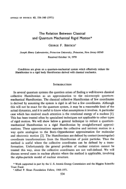
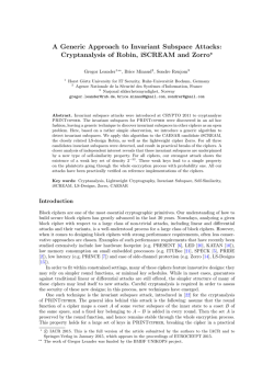
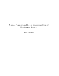
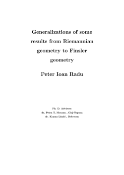

© Copyright 2026